+ All Categories
Home > Documents > A Dynamic Term Structure Model of Central

A Dynamic Term Structure Model of Central

Date post: 10-Jan-2022
Category:
Upload: others
View: 3 times
Download: 0 times
Share this document with a friend
118
A Dynamic Term Structure Model of Central Bank Policy by Shawn W. Staker MASSACHUSETTS INSTITUTE OF TECHNOLOGY AUG 0 7 2009 LIBRARIES Submitted to the Department of Electrical Engineering and Computer Science in partial fulfillment of the requirements for the degree of Doctor of Philosophy at the MASSACHUSETTS INSTITUTE OF TECHNOLOGY June 2009 @ Massachusetts Institute of Technology 2009. All rights reserved. A uthor ............... . Department of Electrical Engineering and Computer Science June5, 2009 C ertified by .... - ---------------- Leonid Kogan Nippon Telephone and Telegraph Professor of Management Thesis Supervisor Accepted by.......... .. ......... ........ Terry P. Orlando Chairman, Department Committee on Graduate Theses ARCHIVES
Transcript

A Dynamic Term Structure Model of Central

Bank Policy

by

Shawn W. Staker

MASSACHUSETTS INSTITUTEOF TECHNOLOGY

AUG 0 7 2009

LIBRARIESSubmitted to the Department of Electrical Engineering and Computer

Sciencein partial fulfillment of the requirements for the degree of

Doctor of Philosophy

at the

MASSACHUSETTS INSTITUTE OF TECHNOLOGY

June 2009

@ Massachusetts Institute of Technology 2009. All rights reserved.

A uthor ............... .Department of Electrical Engineering and Computer Science

June5, 2009

C ertified by .... -----------------Leonid Kogan

Nippon Telephone and Telegraph Professor of ManagementThesis Supervisor

Accepted by.......... .. ......... ........Terry P. Orlando

Chairman, Department Committee on Graduate Theses

ARCHIVES

A Dynamic Term Structure Model of Central Bank Policy

by

Shawn W. Staker

Submitted to the Department of Electrical Engineering and Computer Scienceon June 5, 2009, in partial fulfillment of the

requirements for the degree ofDoctor of Philosophy

Abstract

This thesis investigates the implications of explicitly modeling the monetary policyof the Central Bank within a Dynamic Term Structure Model (DTSM). We followPiazzesi (2005) and implement monetary policy by including the Fed target rate asa state variable. The discontinuous target dynamics are accurately modeled via anon-linear switching process, while still maintaining affine requirements under thepricing measure ensuring tractability. To ensure a flexible risk specification we turnto the parametrization of Cheridito et al (2007), with extensions to the target jumpprocess. Model parameters are estimated via a simulated maximum likelihood es-timation scheme with importance sampling. A Bayesian particle filter is used as arobustness check, and it's use for static parameter estimation in a DTSM frameworkis explored.

Our results support those in Piazzesi (2005), revealing a substantial improvementin pricing errors especially on the short end of the yield curve. The model constructionprovides a natural framework to inspect monetary policy information embedded inyields, which is found to be substantial. We find the addition of the target rate greatlyimproves the model's ability to explain excess return. An ability which is increasedwith the inclusion of the full term structure of target rates, as measured from Fedfuture contracts. We postulate the improved performance is due to the target as aproxy for short term rates, and a conduit to express the information content of theterm structure of target rates.

Thesis Supervisor: Leonid KoganTitle: Nippon Telephone and Telegraph Professor of Management

Acknowledgments

I would like to thank my research advisor Leonid Kogan for his continual support and

never ending patience. I am also grateful to the members of my research committee:

Munther Dahleh, Scott Joslin, and John Tsitsiklis. Much of my work, and most of my

sanity, is due to the invaluable and extensive discussions with Scott Joslin. Teaching

for Munther Dahleh and John Tsitsiklis are highlights of my MIT education, providing

experiences which have shown me my way forward.

I owe a special debt to Andrew Lo for providing me with office space at the

Laboratory for Financial Engineering. A unique collaborative center, supporting a

wide range of bright students and exciting research. Finally if it wasn't for fellow

classmate Amir Khandani, I would have driven myself mad with talk of Q measures.

Though the trials and tribulations associated with this thesis have marked my time

at MIT, the meeting of Tufool Al-Nuaimi has marked my life. I owe her more than I

can ever repay, and love her more than I can say. My academic accomplishments pail

in comparison to the pride I feel in starting a new chapter of my life with the woman

I love. Ahibik b'kul qalbee.

Contents

1 Introduction

2 Dynamic Term Structure Models

2.1 Mathematical Foundation .......

2.2 Affine Term Structure Models .....

3 DTSM of Central Bank Policy

3.1 M otivation ................

3.2 Model Construction ...........

3.2.1 Latent State Space .......

3.2.2 Jump Process ..........

3.2.3 Change of Measure .......

3.2.4 Bond Pricing Coefficients....

3.3 Estimation ................

3.3.1 Simulated Maximum Likelihood

3.3.2 Particle Filtering ........

3.4 Market Data. ..............

3.4.1 FOMC Data............

3.4.2 Libor & Swaps . . . . . . . . .

with. . .. . .

. . .

Importance

...... 0.

3.4.3 Fed Future Contracts

4 Results & Performance

4.1 Estim ation Results ............................

7

23

23

26

31

31

35

36

38

40

43

46

47

50

52

53

53

Sampling

.....

57

57

. . . . . . . . . . . . . . . .

................

4.2 Pricing Errors .. ... . .. ... . .. .. . . . ... . ... . .. .. 76

4.3 Yield Response to Shocks ........................ 83

4.4 Risk Premium ............................... 92

5 Conclusion 103

A Bond Pricing Accuracy Check 105

B Estimation 107

B.1 Simulated Maximum Likelihood ................... .. 107

C Details on Model Extensions 109

C.1 A 1(3) Benchmark ............................. 109

C.2 Term Structure of Target Rates ..................... 111

List of Figures

3-1 Monthly estimates of tracking error with respect to the Fed target rate.

Tracking error is difference in non-overlapping monthly averages of the

Fed target and the Fed effective funds rates. Sample mean absolute

tracking error 2.61 bp, sample vol 4.56 bp. . ............... 33

3-2 Times Series of the Fed target rate, the intended overnight Fed funds

rate set by the FOMC. Changes to the target announced during sched-

uled FOMC meetings (circle), changes to the target announced during

unscheduled FOMC meetings (square). . ................. 34

3-3 Histogram of changes to the Fed target .................. 35

3-4 Time series of the Fed target and a subset of synthetic zero yields... 55

4-1 Estimated values of the stochastic volatility factor Xt. Horizontal bar

fixed at the P measurable long run mean of X 1 . . ............ 60

4-2 Estimated values of the latent state variable X 2 . Horizontal bar fixed

at the P measurable long run mean of X 2 . . . . . . . . . . . . . . . . 61

4-3 Estimated values of the latent state variable Xt. Horizontal bar fixed

at the P measurable long run mean of X 3 . . . . . . . . . . . . . . . . 62

4-4 Estimated values of the latent short rate r(Xt), and the observable Fed

target rate. ................................ 63

4-5 Monte Carlo verification of long run mean of jump intensity. ..... 64

4-6 Monte Carlo estimate of model yields unconditional mean. ...... . 65

4-7 Monte Carlo estimate of model yields unconditional volatility. .... 66

4-8 Monte Carlo estimate of model yields unconditional skew. ...... . 67

4-9 Monte Carlo estimate of model yields unconditional kurtosis...... 68

4-10 Monte Carlo draws of the short rate as a histogram. . .......... 69

4-11 Short dated model predictions of target changes at the next FOMC

meeting. Estimates are maximum likelihood values via a Monte Carlo

generated distribution of 0. ....................... 70

4-12 Decomposition of future expected target changes over the next sched-

uled FOMC meeting, where the y-axis is in units of 25 basis points. Fu-

ture expected target changes are approximately equal to Et[AsS t]h.

Where the next scheduled meeting is at time s and h is the length of

the meeting................................ 72

4-13 Decomposition of future expected target changes over the next sched-

uled FOMC meeting with respect to current yields. Future expected

target changes are approximately equal to Et[Als > t]h. Where the

next scheduled meeting is at time s and h is the length of the meeting.

Correlation is the standard sample correlation on first differences. . . 73

4-14 A time series of out-of-sample pricing errors for near dated Fed Future

contracts .................... ............ 81

4-15 Time series of the number of 25 basis point jumps in the Fed target

rate expected to occur at the next scheduled FOMC meeting. Model

EQ[Jumps] are taken from the model using the optimal model param-

eters of table 4.1. Market EQ[Jumps] are obtained by inverting the

pricing relation for Fed future contracts. . ................ 82

4-16 Loadings for the first three Principle Components of Yields. ..... 83

4-17 Normalized pricing vector. Cx is normalized to display the response

to a 1 standard deviation shock. Co requires no such normalization. 85

4-18 Normalized pricing vector. Cx is normalized to display the response

to a 1 standard deviation shock. Co requires no such normalization. 86

4-19 Time series of model implied monetary policy shocks, as well as shocks

measured via Fed future contracts. Sample correlation of two measures

is 0.7632 .. . . . . . . . . . . . . . . . . . . . . . . . . . . . . . ... .. 88

4-20 Response of Yields to shocks in monetary policy, as measured by unan-

ticipated changes in the Fed target rate. . ................ 91

4-21 Realized one year excess return on {2,3, ..., 9, 10} year bonds using

weekly sampled bond yields. Return calculations use overlapping win-

dows. ................................... 93

4-22 Model expected one year excess return on {2,3, ... , 9, 10} year bonds

using weekly sampled bond yields. Return calculations use overlapping

window s .. . . . . . . . . . . . . . . . . . . . .. . . . . . . . . . . . ... 95

4-23 Explaining excess bond returns. The Benchmark is a A 1(3) model

with no jump component. Ylds indicates the use of model parameters

of table 4.1, which are estimated using yields only. ........... 96

4-24 Plot of the term structure of target rates taken from Fed future con-

tracts during the 2000 turning point. Doted line is the actual Fed

target rate. ................................ 97

4-25 Plot of the term structure of target rates taken from Fed future con-

tracts during the 2005 tightening cylce. Doted line is the actual Fed

target rate. ................................ 98

4-26 Explaining excess bond returns. The Benchmark is a A 1(3) model

with no jump component. Ylds indicates the use of model parameters

of table 4.1, which are estimated using yields only. Ylds & Futures

represents model performance when yields and Fed future contracts

are used to calibrate model parameters. . ................. 99

4-27 Explaining excess bond returns via ordinary lease squares regression.

3PC are the three principle components of all yields of section 3.4.2.

MM indicates the short dated 1 week money market rate. FF indicates

the 1 month ahead Fed Future contract as described in section 3.4.3. 100

12

List of Tables

3.1 Table of changes to the target which were announced during unsched-

uled FOMC meetings. Includes dates from January 1 1997 to January

1 2009 . . . . . . . . . . . . . . . . . . . . . . . . . . . . . . . . . . . . 35

3.2 Percent of total variation explained by the first k principle components,

where the principle component decomposition is performed on yields

(levels) and first differences of yields (changes). . ............ 36

4.1 Point parameter estimates for model parameters of section 3.2. Esti-

mates are calculated via the simulated maximum likelihood technique

described in section 3.3.1. Sample period is from January 1997 to

January 2007, including 521 weekly samples. Standard errors are com-

puted via the product of outer gradients [3]. . ............ . 59

4.2 Half-life of shocks for an equivalent diagonalized system of Xt. Specif-

ically -log(0.5) A-1 , where A are the eigenvalues associated with the

drift matrix of Xt ........................... .. 60

4.3 Long Run Mean of Xt under the Q pricing measure, and the historical

measure P. ............................... 61

4.4 In-sample prediction errors of near dated target changes during sched-

uled FOMC meetings. Maximum absolute prediction error is 25 basis

points ................... ...... ........... 71

4.5 Point parameter estimates. Estimates are calculated via the simulated

maximum likelihood technique described in section 3.3.1. Sample pe-

riod is from January 1997 to January 2007, including 521 weekly sam-

ples. Standard errors are computed via the product of outer gradients

[3]. .................................... .. 74

4.6 In sample pricing errors of yields in basis points. RMSE via map is

found by observing the six month, two year, and ten year yields with

no error and inverting the measurement equation. RMSE via Particle

Filter is obtained by applying the Bayesian Particle Filter of section

3.3.2.................................... 77

4.7 OLS estimates of the coefficients in eq(4.39). Heteroskedasticity-consistent

White t-statistics in parentheses. ................ .... . . . 90

A. 1 Monte Carlo estimates of pricing errors due to linearization of the jump

term and normalization of the meeting schedule. Root mean squared

errors (RMSE) in basis points (pb). MC-ODE is the RMSE of the

difference between the MC yields and the ODE yields. . ........ 106

C.1 Point parameter estimates for the A 1(3) benchmark model. Estimates

are calculated via the simulated maximum likelihood technique de-

scribed in section 3.3.1. Sample period is from January 1997 to January

2007, including 521 weekly samples. Standard errors are computed via

the product of outer gradients [3]. .................... . . . 112

C.2 Point parameter estimates for the target model with information con-

tent of the full term structure of target rates incorporated. Estimates

are calculated via the simulated maximum likelihood technique de-

scribed in section 3.3.1. Sample period is from January 1997 to January

2007, including 521 weekly samples. Standard errors are computed via

the product of outer gradients [3]. .................... . . . 113

C.3 In sample pricing errors for the target model with information content

of the full term structure of target rates incorporated. RMSE via map

is found by observing the six month, two year, and ten year yields with

no error and inverting the measurement equation. RMSE via Particle

Filter is obtained by applying the Bayesian Particle Filter of section

3.3.2 . . . . . . . . . . . . . . . . . . . . . . . . . . . . . . . . . . . . . 114

16

Chapter 1

Introduction

This thesis investigates the implications of explicitly modeling the monetary policy

of the Central Bank within a Dynamic Term Structure Model (DTSM). We follow

Piazzesi (2005) and implement monetary policy by including the Fed target rate as

a state variable. The discontinuous target dynamics are accurately modeled via a

non-linear switching process, while still maintaining affine requirements under the

pricing measure ensuring tractability. To ensure a flexible risk specification we turn

to the parametrization of Cheridito et al (2007), with extensions to the target jump

process. Model parameters are estimated via a simulated maximum likelihood es-

timation scheme with importance sampling. A Bayesian particle filter is used as a

robustness check, and it's use for static parameter estimation in a DTSM framework

is explored.

Our results support those in Piazzesi (2005), revealing a substantial improvement

in pricing errors especially on the short end of the yield curve. The model construction

provides a natural framework to inspect monetary policy information embedded in

yields, which is found to be substantial. We find the addition of the target rate greatly

improves the model's ability to explain excess return. An ability which is increased

with the inclusion of the full term structure of target rates, as measured from Fed

future contracts. We postulate the improved performance is due to the target as a

proxy for short term rates, and a conduit to express the information content of the

term structure of target rates.

Motivation

Our motivation to explicitly include monetary policy into a term structure model

stems from it's well established importance in the wider economy. Changes in the

monetary base directly effect short term rates, and though various intermediaries

effect everything from consumer credit to exchange rates. The Fed alters the monetary

base to meet it's dual mandate of price stability and sustainable economic growth

[36]. The Federal Reserve Bank maintains three controls for monetary policy, all

with the purpose of influencing the daily Fed funds rate. The Fed funds rate is the

overnight interest rate which depository institutions lend balances to other depository

institutions. Based on this description a logical choose would be to use the Fed funds

rate as a state variable reflecting monetary policy. Unfortunately the realized Funds

rate has a number of adverse qualities, principally very high volatility which is found

in many money market rates. As with many money market rates, spikes in the rates

often appear due to known institutional constraints rather than economic drivers.

An alternative choice is to use the publicly announced Fed funds target rate, or

target rate. This is the rate the Fed attempts to steer the funds rate toward via

it's tools of monetary policy. The process in which the Fed conveys the target rate

has evolved with the organization's view on transparency. In 1994 the Federal Open

Market Committee (FOMC) began disclosing changes to it's policy stance. This

evolved in 1995 to a full announcement of the current target level. Communication

tools have evolved since then in an effort to increase transparency, notably in 2000

when the FOMC began to issue assessments on risks to it's dual mandate'. Due

in part to data constraints, our analysis will be limited to a post 1995 time period

where changes to the target rate are publicly announced. Besides the lack of volatility

found in the funds rate, the target is appealing for two broad reasons. The first is

the FOMC's ability to keep the funds rate close to the target rate, which is discussed

in more detail in section 3.2. The second is the unique trait in that the target is not

a market rate, thus it contains no risk premium. As such it may be seen as a proxy

for other indicators of the economy, such as inflation or GDP. This fact will have

1A full description from the Fed's perspective is available at www.federalreserve.gov

interesting implications for risk premium as discussed in section 4.4.

From a mathematical modeling perspective, the target possesses several unique

characteristics with respect to other interest rates. Since 1994 the FOMC has adjusted

the target rate in 25 basis point (bp) increments, and almost predominately at one

of the eight annual FOMC meetings. Incorporating the unique discretized dynamics

and the strong seasonality has the potential to greatly increase the model's ability to

explain observed phenomenon.

From an econometric perspective there have been a number of recent studies lend-

ing support to the importance of the Fed target. One of first studies on yield responses

to changes in the target showed mixed results [16]. Once target changes were decom-

posed into expected and unexpected changes studies found significant yield response

even with long dated maturities [45]. That expected target changes should have no

effect on yields, makes intuitive sense as this information has already been incorpo-

rated into prices. The fact that unexpected target changes, or shocks, effect yields

is a strong motivator for our study. Event studies also provide strong support of

jumps during FOMC announcements, such as [34]. Finally more parametric mod-

els have provided strong support in allowing interest rates to jump during FOMC

announcements, see [43} and [42].

Literature Review

The reported work follows several themes in the current literature. Most notably

are other published studies which explicitly model the Fed target rate within a term

structure model. The most notable of which are [40], [50], and [51]. [40] investigate

a Gaussian term structure model with Fed targeting, where deterministic Fed jumps

are used. [50] build a finite state Markov Chain to characterize target changes, and

find good predictability over a somewhat short sample period.

In particular our work can be seen as an extension of the model in [51], who

uses an affine term structure model with conditionally Poisson jumps driving the

target. Our model uses a richer specification for the jump process, combining a single

time series with a non-linear switching mechanism to drive target jumps. Other

extensions include a more flexible parametric description of the pricing kernel, and

an estimation scheme incorporating a variance reduction technique. We also exploit

a Bayesian Particle filter for a robustness check, and explore it's use for parameter

estimation. Finally our results focus more heavily on model risk premium, and it's

response to the market's term structure of target rates.

Our modeling approach falls within the broad class of Dynamic Term Structure

models (DTSM). To maintain tractability we transform the dynamics under the pric-

ing measure which places the model under the affine variation of DTSM models,

or Affine Term Structure Models (ATSM). [59] and [17] are early examples of term

structcure models, which are now seen as specific examples of ATSMs. The seminal

work which established the broad framework of ATSM models is found in [28] or [27].

Since then [19] and [20] further established the foundations of drift-diffusion ATSM

models which exist today. This framework was extended to in [29] to accomidates

Poisson type jumps. An excellent survey paper on ATSM models is found in [52],

with an equivilant in the DTSM space available in [18]. Finally a comprehensive text

book treatment of DTSM models with an empirical focus is found in [581.

Within ATSM modoels the pursuit of more flexible parametric specifications for

risk premium has been an active subject. An appropriate starting point is the com-

pletely affine price of risk specification in [19]. A slight adjustment in [23] was later

coined semi-affine, followed by essentially affine in [24]. These variations have led to

the fully flexible extended affine configuration of [12], which allows for a price of risk

such that the state space under P and Q are fully flexible affine constructions. This

is the method we apply in section 3.2.3, and later extend for jumps.

A key ingredient to any term structure model is the means to calibrate static

model parameters to historical data, and possibly infer latent state variables. We

will label all such issues under the umbrella of estimation. We identify the two

work horses of ATSM estimation as Method of Moments and Maximum Likelihood.

A comprehensive summary of each method applied to DTSM models is available

in [58]. As the more efficient estimator we focus our efforts on maximum likelihood

techniques. The likelihood function associated with our model dynamics is not known

in closed form and is computationally expensive to construct. This leads us to follow

the existing vein of literature in simulated maximum likelihood (SML) techniques.

This Monte Carlo technique was first presented for drift-diffusion models by [49]. An

excellent empirical comparison of SML techniques with variance reduction techniques

is available in [30]. To reduce the variance in our technique we turn to the importance

sampler proposed in [35], and later formalized in [32].

A significant percentage of ATSM models include latent state variables. Within

the literature a popular means to infer an N dimensional latent state space is to

assume N measurements are observed without error [58]. An alternative is to use

a filtering technique to infer latent states and compute the likelihood function. For

Gaussian systems the infamous Kalman filter is the ideal choice, and a popular ap-

proximation when normality is not present [47]. An alternative to the Kalman filter for

non-linear non-Gaussian systems is the Bayesian Particle Filter. Excellent summary

papers from an engineering perspective are [2, 11], while the technique is presented for

financial problems in [44]. Though flexible and robust, particle filters suffer from high

variance resulting in a discontinuous likelihood functions. A discontinuous likelihood

function with respect to parameters restricts the use of any gradient based optimiza-

tion routines. This trait has greatly limited it's use in static parameter estimation.

Considering this constraint we leverage the filter construction in [54] to quantify the

robustness of our estimates and the ensuing results.

Outline of Thesis

Chapter one contains a detailed presentation on Dynamic and Affine Term Structure

Models, providing much of the background for the following chapters. Chapter two

presents our model construction and further estimation details. The model construc-

tion includes additional details on the Federal Reserve Bank and the model incor-

porates monetary policy. Chapter three contains a full discussion of results, with

emphasis on pricing error and risk premium. We state our conclusions in chapter

four.

22

Chapter 2

Dynamic Term Structure Models

Dynamic term structure models (DTSM) are mathematical models which ensure con-

sistent joint evolution of the yield curve through time. Relative to other modeling

techniques DTSMs provide a consistent framework for cross sectional pricing, exclud-

ing prices which allow arbitrage. They also possess well defined dynamics in time,

allowing characterization of historical changes in the yield curve. Since DTSMs pro-

vide a complete probabilistic model for the yield curve, prices for any fixed income

security may be constructed including derivatives.

In this chapter we provide a brief overview of Dynamic Term Structure Models.

Section 2.1 presents a review of the mathematical foundation from which DTSM

models are based. Section 2.2 introduces the affine class of DTSM models, affine term

structure models (ATSM). To achieve tractability we constrain our model dynamics

under the pricing measure, thus placing the model within the ATSM framework.

Section 2.2 contains background discussions regarding a number of key ingredients

for any ATSM model.

2.1 Mathematical Foundation

Assume the existence of a scalar instantaneous interest rate, r(t), which can be written

as a function of an Markov process, Xt E RN defined on a probability space (Q, F, P).

That is

r(t) --, r(Xt, t) (2.1)

Define a bond as a contract which pays one dollar at time T, and has a time t price

B(t, T, Xt) given by

B(t,T, Xt) = EQ exp -T r(x, s)ds) Ft] (2.2)

Where the expectation is taken over a measure Q, equivalent to P, and Ft denotes a

filtration with respect to time t. Note the functional dependence of B on Xt is a direct

result of the Markovian assumption. Heuristically, the reason to change measure is to

compensate investors for the risk they bear, where Xt may be viewed as risk factors.

Existence of Q and a solution to eq(2.2) is assured under assumptions of no arbitrage,

with regulatory conditions on r and dXt. The discussion of measures is relegated to

section 2.2.

To solve for model implied bond prices, one must solve the conditional expec-

tation in eq(2.2). Possible methods include (i) direct evaluation of the conditional

expectation in closed form, (ii) numerical approximation via a Monte Carlo technique,

or (iii) mapping the conditional expectation to a partial differential equation (PDE)

via Feynman-Kac. Observed prices strongly reject the use of Xt dynamics required

for a closed form solution. Though Monte Carlo is a convenient method to generate

prices, it is computationally prohibitive when calibrating the model. Furthermore

Monte Carlo may be computationally infeasible when Xt is latent, a common trait in

DTSMs. For these reasons the vast majority of research exploits the Feynman-Kac

stochastic representation formula to construct a solution to eq(2.2).

Consider a PDE for T > 0 of the form

Df (x, t) - r(x, t)f (x, t) = 0 (2.3)

with boundary condition f(x, T) = 1

where (x, t) E R x [0, T), and D is an operator which takes the drift component of

the derivative'. The Feynman-Kac probabilistic solution to eq(2.3) is

f (x, t) = Et [exp ( r(Xs, s)ds (2.4)

Now note B(t, T, Xt) = f(x, t). Thus given dynamics for the stochastic process Xt,

eq(2.3) provides a method to compute bond prices. Note the PDE of eq(2.3) has

been restricted to reflect the specific form of eq(2.2), including the unitary boundary

conditions reflecting the one dollar notational value of B(t, T). For clarity we note

the function dependence of B on Xt is often omitted.

To expand on eq(2.3) we require additional structure on Xt dynamics. Assume

Xt is a continuous time drift-diffusion process in RN with the following specification

dXt = p(Xt, t)dt + a(Xt, t)dWt (2.5)

Where dWt is a N dimensional Brownian motion. Substituting the dynamics of

eq(2.5) into eq(2.3) yields

1ft(x, t) + fx (x, t)(x, t) + -tr[a(x, t)a(x, t)T f.(x, t)] - r(x, t)f(x, t) = 0 (2.6)

The solution is also expandable to include the presence of measurable jump pro-

cesses. Assume Xt is a Markov process with drift, diffusion, and Poisson type jump

components.

dXt = p(Xt, t)dt + o(Xt, t)dWt + J(Xt, t)dNt (2.7)

Where Nt is a vector of Poisson jump processes, J(Xt, t) are jump amplitudes, with

each jump process having an associated jump intensity Ai. In general the intensity,

as well as jump amplitude may depend on Xt. Substituting the dynamics in eq(2.7)

'D is also known as the infinitesimal generator, infinitesimal operator, Dynkin operator, the It6operator, or the Kolmogorov backward operator. See [48] for a mathematical presentation, or [4] fora more finanical context.

into eq(2.3) yields

ft (, t) + f(x, t)U(x, t) + -2tr[a(x, t)a(,t)T fx(x, t)] - r(x, t)f(x, t)

+ Ai Ei[f(x + J(x, t), t) - f(x, t)] = 0 (2.8)

where there are i jump components. Details on admissible Poisson jump specifica-

tions, as well as sufficient conditions for existence of eq(2.8) is covered in [15].

If Xt is scalar and observable, then the PDEs of eq(2.6) and eq(2.8) may be

integrated to construct bond prices. State of the art research, including the currently

reported work, focuses on latent Xt E RN where N > 3. As such direct PDE

integration of eq(2.6) and eq(2.8) is computationally infeasible. A well reported means

to achieve a tractable solution, is to restrict Xt dynamics such that the PDEs are

reduced to a system of ODEs. The reduced system of ODEs are easily solved via

numerical integration. As described in section 2.2, this class of models is referred to

as Affine Term Structure Models.

2.2 Affine Term Structure Models

Section 2.1 outlines the general method for constructing a pricing function for bonds.

When specifying state variables, one is often faced with a trade-off between richness

of dynamics and computational tractability. A well reported class of tractable models

are Affine Term Structure Models (ATSM). A dynamic term structure model is affine

if yields are affine in the state variables, or alternatively bond prices are exponen-

tially affine. Tractability in ATSM models is derived from the ability to reduce the

Feynman-Kac PDE into a system of ODEs, which are easily solved via the method

of undetermined coefficients. As reported in [29] any state space which possess an

exponentially affine conditional characteristic function may lead to an ATSM model2 .

Pioneering work in dynamic term structure modeling can be viewed as one dimen-

sional ATSM models[59, 17]. The lack of fit to historical dynamics and conditional

2We also require that r(Xt) be affine in Xt.

moments has encouraged the development of multi-factor or multidimensional mod-

els. Multi-factor ATSMs were originally formalized in [27, 28]. Coverage of ATSM

models for Xt in the multi-factor affine drift-diffusion family is found in [19]. [29]

contains a comprehensive presentation on pricing a wide range of securities which are

driven by an affine jump-diffusion state space. A rigorous mathematical presentation

of general affine processes with applications in finance can be found in [26]. An excel-

lent survey paper on ATSM models is found in [52], while the survey in [18] includes

expanded coverage beyond pricing risk free bonds.

Dynamics Under the Pricing Measure

We begin a brief summary of bond pricing for ATSM models with Xt defined as a

drift-diffusion process. We note all processes in this section are under the Q pricing

measure as defined in eq(2.3). Using the notation of [19] define Xt as

dXt = IC(O - Xt)dt + EfVdWQ (2.9)

where Wt is a N dimensional vector of independent Brownian motions, K: and E are

N x N matrices, E is a N x 1 vector, and St is a diagonal matrix with the ith diagonal

element given by

[St]ii = ai + 3iTXt (2.10)

Assume an affine form for the short rate r(Xt, t) as

r(X, t) = 60 + SIXt (2.11)

and a solution for Bond prices of

B(t, n) = exp(Co(n) - Cx(n)TXt) (2.12)

where n = T - t. Substituting eq(2.9-2.12) into eq(2.6) yields ordinary differential

equations (ODEs) for Co(n) and C,(n).

dC(n) eT T C(n) + -2 -

dn

dCx(n) 1

=d)- TCX(n) + 1 [ETC (n)]20 (2.13)dn 2

with initial conditions Co(O) = 0 and Cx(O) = [0]. For some specifications the ODEs

have closed from solutions, others can be solved via numerical integration.

As discussed in [19], two key issues in specification of the any state space is ad-

missibility and econometric identification. Admissibility is primarily concerned with

ensuring that any component of Xt which has an associated nonzero fi is nonnegative

with probability 1 and thus real valued. This forces constraints within components

of dXt, as well as correlation between components. Econometric identification is con-

cerned with ensuring unique model prices, and identification of all model parameters.

A primary contribution of [19] is to formulate a canonical representation for nested

families of commonly used ATSM models. This representation allows for identification

of restrictive assumptions, thus giving the most flexible model possible.

Work in ATSM models when dXt includes jump components is found in [29, 10].

The admissibility for ATSM models with state variables being defined as affine jump-

diffusions (AJD) includes conditional mean and variance of dXt, as well as the short

rate are affine in Xt. To maintain tractability which is the hallmark of ATSM models,

the jump intensity At and jump amplitude Jt cannot both depend on Xt. Assume

ATSM conditions given for drift-diffusions hold, and extend the state space to include

a jump process. Define the intensity of the jump process to be affine in Xt, At =

A + Ax Xt and specify a constant deterministic jump size v. Then eq(2.8) reduces

to a system of ODEs similar to eq(2.13)

dCT(n) 1()= ETTC_(n) + Z[ETC(n)]2 - 6- A)[exp(v(CO)j) - 1]dn 2

dO, (n) - KCTCn +1 Z T (i)213- dA)dCd(n) Cn

where (Cx)j is the element of Cx which corresponds to the jump process.

Change of Measure

As stated in section 2.1 we identify the measure associated with Xt as P, that is

Xt E RN defined on a probability space ( P, , P). The Q measure is a constructed

measure, such that the expectation of eq(2.2) is equal to bond prices. Since the

seminal work in [38, 391 arbitrage free pricing has been built on the existence of an

equivalent martingale measure Q, often referred to as the risk-neutral measure. See

[4] for an excellent textbook treatment on the arbitrage pricing, and [25] for a classic

though more compact presentation.

Girsanov's theorem provides the machinery to construct a martingale measure

which is equivalent to P. For diffusion processes, Girsonov's theorem allows us to

write

dWt = dWtP + A(Xt)dt (2.15)

for any adapted process A. Define Xt as a drift-diffusion under P

dXt = pf(Xt)dt + a(Xt)dWtp (2.16)

Applying eq(2.15), we find dXt under Q

dXt = [pP(Xt) - a(Xt)A(Xt)] dt + a(Xt)dWtQ (2.17)

The change in drift under Q is the mathematical mechanism allowing investors to

demand additional premium on the return of an asset. For this reason A(Xt) is often

referred to as the price of risk.

To maintain ATSM tractability the moments of Xt under Q must be affine in

Xt, however there is no such restriction under P. Restrictions on the dynamics of

Xt under P are primarily driven by the estimation scheme used to calibrate model

parameters to observed data. A popular choice in the literature is to specify the

dynamics of Xt as affine under Q and P. To this end [12] provides the mathematical

justification for an extended affine price of risk3 . The formulation essentially allows

a fully flexible drift specification under P and Q. As summarized in [57], several

non-affine P specifications have been reported over the years.

Similar change of measure techniques for jump-diffusions have been reported. As

is typical, we define the P measurable jump intensity as an affine function of the state

vector

AP = Ao + A Xt (2.18)

Then we can write the Q measurable jump intensity with respect to any adapted

process A

AQ = AP(Xt) [At(Xt) - 1] (2.19)

Restrictions on At ensure AQ > 0 and is non-explosive. An overview of jump-diffusion

models is found in [56], and [29] reports change of measure requirements for affine

jump-diffusions.

3 [12] show under mild restrictions that At remains non-explosive, and thus is an equivalentmartingale measure.

Chapter 3

DTSM of Central Bank Policy

3.1 Motivation

The Federal Reserve Bank (Fed) maintains a publicly announced target rate for

overnight loans made between depository institutions. Our motivation to include

the target rate within a dynamic term structure model may be categorized into two

areas: economic and mathematical. We find the unique characteristics of the target

rate to be easily incorporated into a dynamic term structure model.

The economic motivation to include the target rate stems from it's use as a key

tool of monetary policy. The Fed provides the following description of monetary

policy and the tools at it's disposal. 1

The term "monetary policy" refers to the actions undertaken by a

central bank, such as the Federal Reserve, to influence the availability

and cost of money and credit to help promote national economic goals.

The Federal Reserve Act of 1913 gave the Federal Reserve responsibility

for setting monetary policy.

The Federal Reserve controls the three tools of monetary policy-open

market operations, the discount rate, and reserve requirements. The

Board of Governors of the Federal Reserve System is responsible for the

1Taken from the website of the Federal Reserve Bank: www.federalreserve.gov

discount rate and reserve requirements, and the Federal Open Market

Committee is responsible for open market operations. Using the three

tools, the Federal Reserve influences the demand for, and supply of, bal-

ances that depository institutions hold at Federal Reserve Banks and in

this way alters the federal funds rate. The federal funds rate is the interest

rate at which depository institutions lend balances at the Federal Reserve

to other depository institutions overnight.

Changes in the federal funds rate trigger a chain of events that affect

other short-term interest rates, foreign exchange rates, long-term interest

rates, the amount of money and credit, and, ultimately, a range of eco-

nomic variables, including employment, output, and prices of goods and

services.

The Fed target rate is a publicly announced goal for the Fed funds rate. Federal

Open Market Operations (FOMC) attempts to steer the daily effective funds rate

toward the target rate, by supplying or withdrawing liquidity [31]. This is carried

out in part by the trading desk of the Federal reserve bank in New York. Market

influences and institutional constraints force temporary deviations, though on average

the Fed has been very successful in keeping the rate at the intended target [9]. Figure

3.1 shows the Fed's monthly tracking error for the period of this study. Using non-

overlapping months we find the mean absolute tracking error to be 2.61 basis points.

The main motivation to use the target rate over the funds rate is the high volatility

of the funds rate, which it shares with most short dated assets.

The combined effect of it's use as a monetary policy tool and short dated reference,

results in the target acting as an anchor for longer dated yields. Figure 3.4.2 shows

a time series plots for the target and a subset of synthetic yields used in our study.

Except for rare times of extreme displacement, the target is seen as an anchor for

longer maturity yields. Finally, several empirical studies have documented that yields

of all maturities respond to unanticipated changes in the target rate [45, 53, 33]. In

summary the economic motivation to include the target rate is it's use in monetary

policy and the interconnected characteristic as an anchor for longer maturity yields.

Fed Target Tracking Error

.

S - 1 0 ... .... .... ... .. .... ... ..... ... ....... .... ..... .. .

- 1 5 ... ... ... .. .... .... ... ... ..... ...

-20

-251996 1998 2000 2002 2004 2006 2008

Non-overlapping Monthly Samples

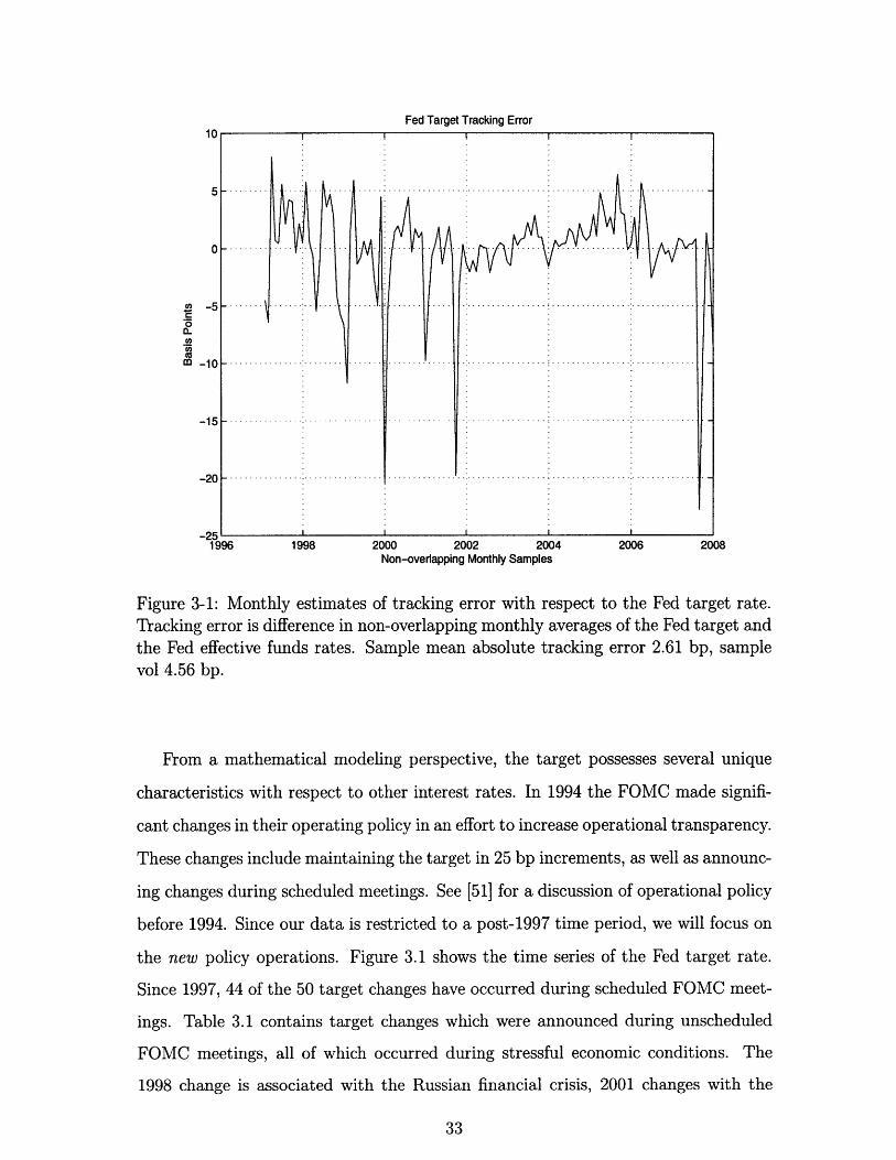
Figure 3-1: Monthly estimates of tracking error with respect to the Fed target rate.Tracking error is difference in non-overlapping monthly averages of the Fed target andthe Fed effective funds rates. Sample mean absolute tracking error 2.61 bp, samplevol 4.56 bp.

From a mathematical modeling perspective, the target possesses several unique

characteristics with respect to other interest rates. In 1994 the FOMC made signifi-

cant changes in their operating policy in an effort to increase operational transparency.

These changes include maintaining the target in 25 bp increments, as well as announc-

ing changes during scheduled meetings. See [51] for a discussion of operational policy

before 1994. Since our data is restricted to a post-1997 time period, we will focus on

the new policy operations. Figure 3.1 shows the time series of the Fed target rate.

Since 1997, 44 of the 50 target changes have occurred during scheduled FOMC meet-

ings. Table 3.1 contains target changes which were announced during unscheduled

FOMC meetings, all of which occurred during stressful economic conditions. The

1998 change is associated with the Russian financial crisis, 2001 changes with the

9/11 terrorist attack and subsequent recession, and the 2008 changes with the recent

sub-prime crisis and ensuing recitation.

Time Series of the Fed target rate

01996 1998 2000 2002 2004 2006 2008 2010

Figure 3-2: Times Series of the Fed target rate, the intended overnight Fed funds rate

set by the FOMC. Changes to the target announced during scheduled FOMC meet-

ings (circle), changes to the target announced during unscheduled FOMC meetings

(square).

As seen in figure 3.1 any model constructed dynamics for the target will require

discontinuous dynamics. As detailed in section 3.2.2 we select a conditionally Poisson

counting process to describe the dynamics of the target. The associated jump intensity

is defined with distinct dynamics for scheduled FOMC meetings and the rare jumps

outside of scheduled FOMC meetings.

34

..

. . . . . . .. . . . . . .. . . . . . .. . . . . .. .

...... Targeto Scheduledo Unscheduled

I

.............................

. . . . .. . . . .. . . .

3

............... (

............

Histogram of Target Changes since 1997'"f

Figure 3-3: Histogram of changes to the Fed target.

Date Changes to the Target (bp)15 Oct 1998 -2503 Jan 2001 -5018 Apr 2001 -5017 Sep 2001 -50

22 Jan 2008 -75

08 Oct 2008 -50

Table 3.1: Table of changes to the target which were announced during unscheduled

FOMC meetings. Includes dates from January 1 1997 to January 1 2009.

3.2 Model Construction

In this section we describe the construction of a four factor dynamic term structure

model with explicit modeling of central bank policy via the Fed target rate. The

model construction closely follows that of [51]. The model possesses three latent

state variables, as well as the observable target rate. The latent state variables are

I

-75 -50 -25 0 25Target Changes in Basis Points

.............

. . . . . . ... . . . .

............

.. . .. .

50 75

continuous drift-diffusions, with stochastic volatility via a single CIR process. The

observable target rate possesses a stochastic state dependent jump intensity during

scheduled FOMC meetings, and a low constant intensity outside of scheduled meet-

ings. We infer the latent states by identifying three observables yields to be error free,

and identify optimal model parameters via a simulated maximum likelihood scheme

with importance sampling. Finally we present the workings of a Bayesian Particle

filter, which is used to verify robustness of the estimation method.

3.2.1 Latent State Space

In the seminal paper of [46], a principle component analysis of yield data reveals that

three components explain the vast majority of variation in yields. Table 3.2 shows

the amount of total variation explained by the first five principle components. This

empirical fact has lead the research community to focus on three factor models when

reporting on DTSM models 2. This is especially true when working with latent state

spaces, as additional variables present data fitting issues.

k Yields in Levels Changes in Yields1 93.396 91.1492 99.700 97.6713 99.954 99.3654 99.995 99.7065 99.999 99.849

Table 3.2: Percent of total variation explained by the first k principle components,where the principle component decomposition is performed on yields (levels) and first

differences of yields (changes).

Motivated by the principle component findings we construct our latent state space

with three state variables, denoted by Xt = [X, X2, Xft]. Each state variable is a

continuous drift-diffusion process with the following dynamics

dXt = ppP(Xt)dt + a(Xt)dWtP (3.1)

2Attempts to model specific characteristics of yields often lead to additional state variables, such

as the goal of fitting very short dated yields or money market rates.

where

k P kP o o0P(Xt) = KP' + K P" X t = kP + kP kP kP Xt (3.2)

0 3 31 32 33

and

SX 0 0

a(Xt) = 0 1 + b21 Xt 0 (3.3)

0 0 0l/ + b31Xt

where WtP are Wiener processes under the data generating or historical measure P.

X1 is a square root or CIR3 process, which results in Xt' possessing time varying con-

ditional volatility4 . The construction of a(Xt) then couples the stochastic volatility

to the other state variables. The off diagonal terms in the K P drift component allow

for full flexibility with respect to correlation between state variables. Admissibility

constraints are required to ensure Xt > 0, and thus u(Xt) remains real valued. These

constraints include

1. The two zeros in the first row of K P

2. kP > 0.5

3. bjl > 0 for j = 1,2

In the language of [19], Xt is a A 1(3) model. The notation implies only one state

variable is allowed to drive instantaneous conditional volatility, where there are three

state variables in total. Staying within the drift-diffusion framework and using this

notation, possible model choices for Xt include Ao(3), A 1(3), A 2(3), and A 3 (3). Ao(3)

is unique in that a is a matrix of constants, resulting in Xt possessing a convenient

joint Gaussian distribution. The positives for an Ao(3) model include it's superior

3 The seminal paper of [17] presented the dynamics for the first time in a term structure framework.4 Unless otherwise stated time varying volatility and stochastic volatility are used interchangeably,

as is conditional versus unconditional volatility

ability to fit the yield curve and capture risk premium5 . The overriding negative

feature is the resulting constant conditional variance in model yields, which is strongly

rejected by empirical studies of fixed income data. All Aj (3) models possess stochastic

volatility in Xt, which is then inherited by model yields. The downside of constructing

stochastic volatility is admissibility constraints in the drift of the stochastic driver,

i.e. the zeros in the first row of K'. Such constraints decrease drift coupling, which

is viewed as an important characteristic of high preforming models. Not surprisingly,

the number of restrictions increases with j. The A 1 (3) model is chosen as the most

flexible construction, which accurately reflects time varying volatility in observed

yields. See [19] for one of the initial discussions on this topic, and [20] for a broader

discussion on the Aj(n) framework.

3.2.2 Jump Process

Following section 3.2, model dynamics for the target rate are discrete valued and move

predominately during scheduled FOMC meetings. In line with [51], we select a Poisson

jump process as the kernel to construct target dynamics. During scheduled FOMC

meetings Poisson jumps possess a stochastic intensity driven by all state variables,

while outside of scheduled meeting days jumps are driven by a small constant intensity.

For convenience of presentation define the target rate as Ot, and a superset of state

variables as Xt = [Ot, Xt]T where Xt = [XI, X 2 , X3]T as defined in section 3.2.1.

Heuristically we view Xt as key indicators of the general economy, as such they

should influence the decision making process of the FOMC committee. Mathemat-

ically we implement this relationship by defining the jump intensity as an affine

function of Xt. We can also view the current target rate as an additional proxy for

the state of the economy. For example a historically low target rate would increase

the probability that the Fed is currently attempting to expand the monetary base in

order to provide credit and spur growth. This type of economic information imbedded

in the target level, may or may not be contained in Xt as such we expand the jump

5Risk premium, bond returns, and excess return are used interchangeably. Excess return is the

return one gains from holding a bond, over the promised yield available in the market.

intensity to include Ot.

As shown in figure 3.1 the target moves in increments of 25 basis points (bp). A

continuous time setting implicitly allows the jump process to register several jumps

over any finite period of time, accommodating any net change equal to a multiple of

25 bp. The strict definition of a (compound) Poisson process must be extended to

allow the target to increase or decrease. In [51] this is accomplished by constructing

two competing Poisson process, one with positive jumps and the other with negative

jumps. Unfortunately with this construction ensuring non-negative jump intensities

in an affine framework is not possible. To circumnavigate this difficulty we implement

a non-linear switching mechanism. We formalize this description as

dOt = sign (At) J0dN P for t E scheduled FOMC meeting (3.4)

where the intensity of dNP is equal to A'P = AP + AOt + A Xt , and J6 is equal

to 25 bp. Note when AP is positive Ot may only jump up, and when AP is negative Ot

may only jump down. Unlike in a competing Poisson process framework, our jump

intensity is strictly positive by construction. How we handle the non-linearities of

eq(3.4) when constructing bond prices is discussed in section 3.2.4.

Outside of scheduled FOMC meetings we could use a similar construction as in

eq(3.4). However since jumps outside of scheduled meetings are so rare, the dynam-

ics would have to be different. On possibility is to follow eq(3.4) with A scaled

drastically downward. This would allow the state of the economy, Xt, to influence

the unscheduled jumps while ensuring they are probabilistically rare. However the

unscheduled jumps are so rare, as to force the scaling factor to zero. We instead

choose a more parsimonious framework, allowing jumps during unscheduled meetings

to occur according to a small constant intensity. Specifically outside of scheduled

FOMC meetings we construct the following dynamics for Ot.

dOt = Jo (dNt' - dNtd) for t scheduled FOMC meeting (3.5)

where the jump intensity of dNt' and dNd is equal to A, and J0 equals 25 basis points.

Note we do not observe dNt or dNtd separately, rather we observe the difference.

3.2.3 Change of Measure

Recall the bond pricing relation of eq(2.2)

B(t, T, Xt) = EQ [exp - r(X, s)ds (3.6)

which gives model bond prices as the expectation of a functional under the Q measure.

The dynamics of the state variables specified in section 3.2.1 and 3.2.2 are under the

data generating or historical measure P measure. To transform eq(3.6) into a useable

form we require state space dynamics under the Q measure. We address change

of measure issues for the continuous latent state space Xt, and the discontinuous

observable Ot separately.

With respect to the latent state space Xt, we turn to the extended affine market

price of risk as reported in [12]. Recall Girsanov's theorem applied to a drift-diffusion

transforms the drift, but keeps the diffusion component unchanged.

dXt = ,P(Xt)dt + a(Xt)dWtP (3.7)

= Q(X)dt + a(Xt)dW (3.8)

where in general

pQ(Xt) = p P(Xt) + a(Xt)A(X) (3.9)

where A(Xt) is often referred to as the price of risk. To appreciate the significance

of this label, we note for ATSM models the drift component typically dominates

the pricing function. Combine this characteristic with the heuristic view of U(X)

a measure of risk in state space or economy which it represents. Thus the change

of measure adjusts prices by injecting a scaled measure of risk into the drift of Xt.

Hence A(Xt) is the price of risk. Finally we remind readers that the existence, or

requirement, of the Q measure is given by the fundamental theorem of arbitrage free

pricing [38, 39].

A significant component of recent literature has focused on exploring admissible

parametric forms for A(Xt). Admissibility essentially focuses on ensuring the Q mea-

sure is a martingale and is equivalent to P. Recently [12] reported on a specification

of A(Xt), which allows the most flexible drift under P and Q. For the dynamics given

in section 3.2.1, the parametric form of A(Xt) is

At 02'K + (k- ) + k22 2)+( kQ -P) (3.10)/1\+b 2 1 X1

k( -k P QP Q -kP

L/l+b31lXl

Combining eq(3.10), eq(3.9), and eq(3.1) yields the dynamics of Xt under Q

dXt = Q(Xt)dt + P(X,)dW Q (3.11)

AQ(Xt) = KY + K Q " X t = 0 + kQ kQ kQ " Xt (3.12)

Admissibility of the CIR process requires the zeros in the first row of KQ, as well as

kQ > 0.5. The zeros in KY are due to identification reasons. If we define the short

rate as a fully flexible affine function of 1 t

r(Gt) = P" + P- t (3.13)

then the zeros of Ko are required to uniquely identify po. This requirement is linked

to our choice of calibrating model parameters to yield data. Using alternative observ-

ables, such as derivative data, allows identification without such restrictions.

Change of measure for Poisson type jump processes is well developed, but less

covered in the financial literature. An overview of jump-diffusion models is found

in [56], and [29] reports change of measure requirements for affine jump-diffusions.

When focusing on a change of measure it is often convenient to transform a Poisson

process to a compensated process.

dN P = pP(X)dt + d MP (3.14)

where MR = N P - fo APds, and AP is the (time varying) jump intensity of N P . This

decomposition allows us to write the jump process in terms of a drift term and a zero

mean non-Gaussian innovation, dM P . For the dynamics of section 3.2.2 the drift of

the compensated process is

P(X) = 0 for t 0 scheduled FOMC meeting (3.15)

P(Xt) = (AP + AXXt)dt for t e scheduled FOMC meeting (3.16)

Similar to the drift-diffusion case we construct an equivalent measure by transforming

the drift of dMfP . Since the drift of dMtP is linked by construction to AP, this results

in a new specification for At under Q. The most flexible change of measure for the

jump process results in

A = AQ + AQOt + AQX, (3.17)

where AQ is a three dimensional row vector. There are two important conversations

regarding eq(3.17). One concerning our ability to identify risk premium for the jump

process, when so few jumps are observed. The other involving issues of unbounded-

ness.

If we estimate model parameters using the full data set available, we observe 96

scheduled FOMC meetings out of 626 observations. This implies very low inference

with respect to the P measurable jump intensity. Note the Q measurable jump

intensity of eq(3.17) affects yields at each of the 626 observations. Furthermore during

the 96 scheduled meetings, we observe only 44 target changes. This results in low

inference with respect to jump risk premium. Due to the low inference we'll assume

zero risk premium for the initial models. Section 4.1 explores various risk premiums

for the jump process, and explores if the data supports such specification.

3.2.4 Bond Pricing Coefficients

Within the DTSM framework developing an useable form for model bond prices is

focused on solving the Feynman-Kac PDE of eq(2.8), which is associated with the

conditional expectation of eq(2.2). Along with the dynamics of section 3.2.3, we

require parametric forms for the short rate r(Xt) and the bond prices B(t, T, Xt)

themselves. Given all the required ingredients we must then find a solution to the

PDE of eq(2.8). If standard ATSM protocol is followed the PDE will reduce to a

system of ODEs. Within our model framework the resulting ODEs must be solved

via numerical integration.

Follow ATSM protocol and define the short rate as an affine function of state

variables.

r(X) = pX = po + PO + pxX (3.18)

where Px is a three dimensional row vector. Assume an exponentially affine function

for model bond prices

B(t, T, X) = exp (Co(t, T) - C(t, T)X) (319)

where Cy(t, T) is a four dimensional row vector.

We first take the case when we are not in a scheduled FOMC meeting, t ' FOMC.

During this regime the jump process is given by (4.17), and Xt dynamics are as defined

in section 3.2.3. With these substitutions we can write eq(2.8) as

o0- OB(t, T, X) +B(t, T, X)Q (3.20)0 = + (X) (3.20)-trace X X- r(X)

2 aX 2

+ [B(t, T,X, + J) - B(t, T,)]

+ [B(t,T,X,O- Jo)- B(t,T,.)

Expanding all terms in (3.20) results in a PDE which can be expressed as a an affine

function of X. Since eq(3.20) must hold for all values of X, each coefficient in the

affine representation must separately equal zero. This is the basis of the often quoted

method of undetermined coefficients. The five ODEs which result from eq(3.20) are

dC 1dt Po - CxKox - - (C2 C3) + [2 + exp(JoCo) - exp(-JeCe)]

dCodt p

dCxl 1dxt - Pi + Cx1 K11 + CX2K 21 + CX3 K3 1 - 2 (C 1 + b21C 2 + b31C 3)dCx2

dtdCt3dCx = P3 + CX2 K23 + CX 3 K33 (3.21)

dt

We solve the system of ODEs numerically, via the Runge-Kuttta Method'. Specifi-

cally the integration is started at t = T, where Cy (T, T) = 0 for all j and continued

until t = 0.

For time during scheduled FOMC meetings, t e FOMC, the jump dynamics

6dc can be easily solved analytically.

change to reflect the now stochastic jump intensity of eq(3.4). The resulting PDE is

OB(t, T, X) OB(t, T, X)0 = + (X) (3.22)at aX

+ trace 02B(t, T X) (X)U(X)T - r(X)

+ A(X) I[B(t, T, X, 0 + sign(A(X))Jo) - B(t, T, X)]

Unfortunately the non-linear terms originating from the jump term prevent expressing

eq(3.22) as an affine function of X. To maintain the tractability which is the hallmark

of ATSM models, we linearize the jump term of eq(3.22). Specifically we apply a

Taylor Series expansion

A(X)I [B(t, T, X, 0 + sign(A(X))Jo) - B(t, T, X)]

JoA(X)Co(t, T)B(t, T, X) (3.23)

which is affine in X since A(X) is affine by construction. With this approximation

we are able to reduce eq(3.22) to the following system of ODEs for t E FOMC

dt - Po - CxKol - (C 2 23) - JOoCodt 2

dCO= Po - JoAeCo

dCxldt = pl -+ CxlK11 + CX2K21 X3 Cx3 1 -t- b21 C2 + b31C3) - JoA1Co

dtdCx 3 _dCX3= 3 + CX2K 23 + CX3K33 -JoA 3Co (3.24)dt

The effect of the linearization in eq(3.23) is quantitatively measured in Appendix

A. Unless otherwise noted the approximation is seen to have no noticeable effect on

results, or conclusions drawn from results.

To construct pricing formulas we use the public meeting schedule of the FOMC

to alternate between eq(3.21) and eq(3.24). Begin with the boundary condition

{Co(T, T) = 0, C:(T, T) = 0}, and integrate backwards in time until a FOMC meet-

ing is scheduled. Use the integration result of eq(3.21) as the initial condition to the

integration of eq(3.24). Continue alternating between systems of ODEs until t = 0,

at which point {Co(t, T), Ck(t, T)} is available.

Unfortunately the FOMC meeting schedule changes each year, and is not uniform

within the calender year. This irregularity of the meeting schedule forces us to resolve

the ODEs at each observation and for each bond maturity. Within the context of an

estimation scheme, the resulting computational burden is essentially infeasible. To

alleviate the burden, we follow [51] and assume a uniform meeting schedule after the

first meeting for each observation. The FOMC meeting schedule is known one to two

years in advance, thus for market participates are not aware of the schedule for longer

maturities. This fact lends support to normalize the meeting schedule. Appendix A

quantifies the effect of this approximation, which is minimal for the maturities in our

data set.

3.3 Estimation

A maximum likelihood scheme is chosen to estimate model parameters. Since three

state variables are latent, we identify three observables as error free allowing us to

infer the value of the latent variables by inverting the measurement equation. Since

the transitional density of the state vector is not available in closed form, a simulated

likelihood technique is employed. To speed up the convergence of the Monte Carlo

integration an importance sampling density is exploited. Finally, to verify the esti-

mation results are robust to the inferred latent state variables, a Bayesian Particle

Filter is applied using the optimal model parameters.

We identify weekly sampled six month libor, and {1, 2,3, ... , 9, 10} year swap

contracts as observables. To construct bond prices from the non-linear swap con-

tracts we keep unobserved forward rates constant, resulting in synthetic yields, for

{.5, 1, 2, ..., 9, 10} year maturities. The benefit of synthetic yields is a measurement

equation linear in X.

The log-likelihood function we seek to maximize is

T T

E fy(ytIyt-;) = 1(g(Yt,Y) I g(vyt-1,7Y);7Y) vg(Yt,Y7) (3.25)t=1 t=1

where y is a vector of unknown model parameters, Xt = g(Yt, y) is the inverted

measurement equation, fg ('') is the log conditional density of X, and I V g(Yt, 7y)

is the Jacobian of the measurement equation. Unfortunately the dynamics of Xt do

not permit a closed from expression 7 for fk(-I.). To overcome this obstacle, simulated

maximum likelihood is employed.

3.3.1 Simulated Maximum Likelihood with Importance Sam-

pling

Simulated maximum likelihood (SML) is a popular means to estimate model param-

eters of a continuous time stochastic process using discretely sampled data. The

general idea of SML is to approximate the true conditional density by discretizing

the SDEs of eq(3.1,4.17,3.4) using a Euler approximation and employing Monte Carlo

to estimate the value of the conditional density. Details of the SML technique as pre-

sented by [49] can be found in Appendix B.1. The estimation scheme implemented

is of the SML flavor, with variance reduction achieved via an importance sampling

technique.

View the conditional density f(ytlyt-1; y) as a marginal density, with a corre-

sponding joint density which explicitly depends on the value of y, for s E (t - 1, t).

That is

f (ytIyt-i)= f(yt, YIyt-1)dyt (3.26)

where the y dependency has been dropped for notational simplicity. If a change of

measure is implemented via an importance sampling density fs(y*), eq(3.26) can be

7 Closed form solutions are known for a few special cases, namely Gaussian and square root

diffusions.

written as

f(y -J f(YtY Yt-1) f (y;)dyt* (3.27)f(ytlyt-1) = f f(yt)

Evaluate eq(3.27) using Monte Carlo to find,

M(ytlYt-1) = -- f yt, I fs i) (3.28)j=1

As noted in [32], SML can now be viewed as setting the sampling density to f(y* Iyt-1),

thus 1 hu f(ytly,j1yt-i) J

f M (ytlt-1) 7J f(ylyt-) (yty,Yt-1) (3.29)

j=1 j=1

Though conceptually and numerically simple this sampling density does not exploit

the known realization of yt. A more efficient sampling density is based on the work

introduced in [35]. Let ft be the mode of logf (yt, yt yt-1), and Et be the negative

of the Hessian of logf (yt, tI yt-1) evaluated at it's mode. The proposed importance

sampling density is a multivariate Student-T density with mean pt and dispersion Et.

We denote this sampling density as fT(yt fit, t, v), where v indicates the degrees of

freedom. The importance sampling density estimator is then

fM(Yyt) = f , -) (3.30)

Yt*,j - fT(YtIfit, t, I) (3.31)

which completes the importance sampling scheme. The use of a Student-T density

provides fat tails, with v giving the means to ensure the sampling density has adequate

coverage in the tails as compared to the true density. If the true density f (ytlyt-1) does

not have significant mass in the tails, a multivariate normal may be used in place of

the Student-T. A comparative empirical study on SML techniques using importance

sampling is found in [30] 8. For a drift-diffusion state space, as specified in section 2.2,

the only remaining issue is the discritization used between observations which is the

8 [30] is accompanied by an informative correspondence amongst the principle authors, and the

original authors of each technique.

integer value of M in appendix B.1. For weekly observed data, [32] report empirical

support for using daily discritization, that is M = 7.

Our model has the added complication of one state variable possessing pure jump

dynamics. One option is to follow [51] by expanding the SML of appendix B.1 to

model dOt with Bernoulli random variables. We instead use a solution which lever-

ages the fact that Ot is fully observable at a daily frequency. Note the conditional

density of )Xt can be conveniently split into a continuous and discontinuous compo-

nent. Specifically

fA(st It- 1) = fx(xt Ixt)fo(OtIxt-1, t-,_) (3.32)

For observations where there is no scheduled FOMC meeting E (t, t - 1] the jump

term is defined by eq(4.17). Due to the lack of available data we fix A to it's historical

value. Fixing A means that fo(Otzxt-1, Ot-l) is not a function of 7, and thus does not

influence eq(3.25). Thus our importance sampling scheme for f:(itl t-1) is

J f (xt, x,fItt)j 1(3.33)X j=1 fT(x,t, At, V)

For observations where there is a scheduled FOMC meeting E (t, t - 1] the jump

term is defined by eq(3.4). Since the intensity is a function of X, it will affect the

maximization of eq(3.25). Fix the length of any scheduled FOMC meeting to one

day, and observe Ot at a daily frequency. Focusing on days with a scheduled FOMC

meeting we find eq(3.30) becomes

f(Zt*jlxt-1) 8

f(r-tt-1) = - ' fT(xtIxt ) exp (-IA(x:, ,90)I) A(x,, O)k (3.34)

where k equals the number of 25 basis point jumps during the scheduled FOMC

meeting, and s is the time index directly before the day of the scheduled meeting.

Note eq(3.34) is implicitly holding X constant during the actual FOMC meeting.

3.3.2 Particle Filtering

A popular sequential Monte Carlo (SMC) estimation technique is the particle filter

(PF). Particle filters were first introduced by [37] as a means to estimate a nonlinear

non-Gaussian latent state space. Though particle filtering is well reported as a means

to infer latent states, the use of the technique for model parameter estimation is an

open topic of research. In the current reported research we employ particle filtering

as a means to verify robustness in the choice of yields used to invert the measurement

equation.

For a gentle textbook introduction to the concepts of sequential bayesian inference

and particle filters in particular see [55]. An extensive review of recent research on

Bayesian Filters is found in [11], and with a focus on particle filters in [2]. The edited

volume of [22] contains text book summaries of recent research, including extensions

for parameter estimation. For a dense text book treatment of nonlinear filtering and

estimation of latent states see [8]. A brief review of particle filters applied to financial

econometric problems can be found in the survey paper of [44].

Employing Bayes rule we can express the conditional density of Xt given all ob-

servations up to time t or Y:t as

P(P(Yt I)P(xtlYl:t-) (3.35)P(YtlYl:t-)

In the language of filtering: p(xtYj:t) is the filter density, p(xtlyl:t-) is the predictive

density, and p(ytlxt) is the likelihood density. The predictive density is linked to the

filter density via the state transition density p(xtlxt_1) as

p(xtyt-) = P(xtxt-1)p(xt- lyt-1)dxt-1 (3.36)

The signature of any particle filter is to approximate the continuous distribution

p(xtYl:t) as a discrete probability mass function (PMF). Each particle is a point of

mass in the PMF,N

(xtlyi:t) = (x - xit)(x (3.37)i=l

50

where N is the number of particles, and 6 is the Dirac delta function. Substituting

eq(3.37) into eq(3.36) allows us to evaluate the integral as a summation.

P(XtjYj:t- -= IP( Xt _l)7rtl( t=1i=elds

Substituting eq(3.38) into eq(3.35) yields

(3.38)

(3.39)tl:t) P( l ) =1

i=1

where the typical p(ytjyl:t-1) integration constant is omitted, as it is easily estimated

via normalization. The idea behind particle filters is to use eq(3.39) to draw samples

of (xtlyl:t). The strength of the technique is the novel method in which these draws

are taken. We will focus our attention on the Sampling Importance Resampling (SIR)

algorithm of [37].

SIR Particle Filter: given particles and weights at time t-1: [{ l, }i 1

1. Draw x p(xtz _i)

2. Calculate wt = p(ytlx )

3. Normalize weights; wt = =- W

4. Resample particles xt based on i) to yield [{x, w} i1], where w - .

Repeat for t + 1, t + 2,..., T

See [11] for a summary of reported resampling techniques, including systematic re-

sampling which is used in this reported work. Note the SIR algorithm only requires us

to draw from the transitional density, and to evaluate the likelihood density. Given

dynamics for a state space we can (almost) always take draws by the transitional

density, even though evaluation of the density may be computationally prohibitive

or infeasible. The likelihood function, as defined above, is given solely by our mea-

surement equation and based largely on the assumed (additive) error. Thus particle

filters are extremely flexible, and appropriate for our state space construction.

As with other filtering schemes many metrics of interest are conveniently available.

Estimates of latent Xt are available from the filtered density p(xt yt), typically the

expected value. The Monte Carlo estimate of the likelihood function is

L(ytlyl:t-1) = P(Ytlxt)p(xtyt-1)dxt (3.40)

N

SZP( (ytlxt)wt (3.41)i=1

NEP(yt x() (3.42)i=1

Unfortunately the likelihood estimate has a high amount of variance due to the resam-

pling step. This variance results in a likelihood which is discontinuous with respect

to -y. Discontinuous likelihoods mean gradient based optimization routines cannot be

used.

3.4 Market Data

Model parameter estimation, as well as model performance evaluation, requires sev-

eral pieces of market data. To create market implied zero yields we require LIBOR

rates and swap rates. The model uses the Fed target rate as an observable state

variable, and requires the FOMC meeting schedule to construct the pricing equation.

We will also have need for a metric of market implied expected target changes, which

is derived from Fed future contracts. The data collected spans almost 11 years, from

January 7th 1997 to December 30th 2008. The lower date being bounded by the

author's access to swap rates, though institutional changes would limit the data to

1994 if available.

Ideally all observations would be recorded with a uniform time and date stamp.

Unfortunately, with the author's current data sources, this is not possible. As such we

implement time shifts and minimize temporal misalignment by sampling at a weekly

frequency. In summary we shift all data to the London market perspective.

3.4.1 FOMC Data

The estimation scheme of section 3.3.1 requires daily sampling of the Federal Reserve

target rate, while the pricing function requires weekly samples. Since 1994 changes to

the target are announced during the afternoon in New York, typically at 2:15PM EST.

A time series of Fed target rates is available from DataStream[21], where changes to

the target are time stamped the day they are announced. To link the target rate to

the London time stamp of yields, we increment all target dates by one business day.

This eliminates the error with target rates as the rate recorded at 5:00PM EST is the

prevailing target rate used for all trading activity on the following day in the London

market. Alternatively one may note that when changes to the target are announced

at 2:15PM EST, the London Market is closed, hence this change will not be reflected

in the LIBOR or swap rate of the same date, but rather the rate of the following

business day.

The dates of all FOMC meetings since 1970 are available via the Federal Reserve,

including a tentative schedule for the following two years9. Scheduled FOMC meetings

last one or two days, though any change in the target rate is almost always announced

in the afternoon of the second day. Unscheduled meetings occur when the the FOMC

announces a target change, and there is no scheduled meeting. Hence unscheduled

meetings are easily identified by comparing changes in the target time series and the

meeting schedule. Consistent with incrementing the target time series by one business

day, we increment scheduled FOMC meetings by one business day. See [45] and [33]

for additional information regarding unscheduled target changes.

3.4.2 Libor & Swaps

Zero yields are constructed from a six month libor rate, as well as {1, 2, 3, ..., 9, 10}

USD swap rates. Libor is obtained from DataStream, who in turn receive the rate

91n particular the Federal Reserve Bank of Minneapolis [6] maintains a website with easily ac-cessible data.

from the British Bankers Association (BBA). The LIBOR rate used is an average

price from major Banks in the London Market, recorded at 11:00AM London local

time1 . The relationship between a zero bond B(t, T) and a Libor rate L(t, T) is

B(t, T)= (3.43)1 + L(t, T)T(t, T)

where T(t, T) is the day count over T - t, approximately 0.5 for a six month rate.

Swap rates are obtained from DataStream, who in turn receive the rate from ICAP.

The swap rates are USD dominated, recorded at 5:00PM London local time, and are

priced to reset twice a year (semi-annual). The relationship between a zero bond

B(t, T) and a semi-annual swap rate S(t, T) is

1 = B(t,T) + E B(t, t + (3.44)j=1

The left hand side of eq(3.44) is the present value of the floating leg of the swap,

which is always equal to the notional value of the underlying. The right hand side

represents the present value of the known fixed payments over the life of the swap.

To construct the (synthetic) zero yield curve we bootstrap mid-year zero bonds by

holding forward rates constant. See [41] for a textbook presentation on bootstrapping

techniques, including constant forward rate methods.

3.4.3 Fed Future Contracts

A 30-day Fed funds future contract (Fed future) requires delivery of the monthly

average Fed funds interest rate paid on a principal amount of $5 million. In practice

the contracts are marked to market, or cash settled on a daily basis avoiding any

payments at the contract's expiration. Fed futures settle on the last trading day of

10 DataStream gives the following description, "The BBA LIBOR Fixing is based upon rates

supplied by BBA LIBOR Contributor Panel Banks. An individual BBA LIBOR Contributor Bank

contributes the rate at which it could borrow funds, were it to do so by asking for and then accepting

inter-bank offers in reasonable market size, just prior to 11:00 hrs. Contributor rates are ranked

in order and the middle two quartiles averaged arithmetically. Such average rate will be the BBA

LIBOR Fixing for that particular currency, maturity and fixing date".

Fed Target and Zero Yields

S.iSA

4 F-............

i . . . . 'A, i

SI

target-.- 6m

-- - 2yr5yrlO10yr

I

1996 1998 2000

.2

2002 2004 2006 2008 2010

Figure 3-4: Time series of the Fed target and a subset of synthetic zero yields.

the month in which they expire, with a settlement rate 1 equal to the arithmetic

average of the funds rate for the expiry month 12. Contracts are actively traded for

the current month or spot month, as well as 1 to 2 months ahead. Contracts up to

24 months in maturity do exist, though the volume is usually thin and often zero [9].

Fed fund futures are convenient tools to measure the market's expectation of

changes to the target rate. An illustrative example follows. Assume you buy the spot

month Fed future contract on 3/21/2002, which expires in April 2002. The target rate

on 3/21/2002 was 1.75%, and the next scheduled FOMC meeting was on 5/7/2002.

The futures contract should be approximately equal to $100 - 1.75 = $98.25, which

indicates the market's expectation that the target rate will not change in April 2002.

"Contracts are priced as 100 minus the settlement rate.12For weekend and holidays the rate on the previous trading day is carried over

..... . .

. . . . . . . . . . . . . . .

If there is at most one FOMC meeting per month, Fed futures can be used to extract

the market's expectation of target changes at FOMC meetings.

In general the time t price of the spot Fed future contract, denoted by fmt, is given

by

t 1ftm = 100 - { ri + - E-t E ri} (3.45)

i=1 i=t+1

where ri is the daily Fed funds rate and m is the total number of days in the month.

The Fed has historically been able to keep the average Fed funds rate within basis

points of the target [36]. This documented fact leads one to approximate any finite

sample mean of the Fed funds rate by the target rate over the sample. If one then

assumes the target is moved only during a FOMC meeting, eq(3.45) provides a con-

venient means to estimate the market's expectation with respect to changes in the

target rate.

A few points are worth mentioning. The right hand side of eq(3.45) could also

contain a risk premium, to compensate a person for holding the risk associated with

the next m - t days. [53] and [13} find evidence of a small risk premium on the

order of a few basis points at a one month horizon. Also note that eq(3.45) is for the

current spot month. If t is in the 2nd half of the month, there is a meeting before the

end of the month, and there is no meeting scheduled for the following month the one

month ahead future is used instead of the spot month. There are two main reasons

for this strategy. As t --, m target changes will have less of an effect on the months

average, and daily fluctuations in the Fed funds rate will add noise to the estimate of

the expectation. It's also been noted that spot contract volume decreases drastically

as t -+ m, which reduces the information content of the contract [9], [1].

Chapter 4

Results & Performance

In this chapter we report on model results and performance. We begin with estimation

results, including point estimates for all free model parameters. We present a full

characterization of the associated state space, with emphasis on contributions to

the short rate and jump intensity. We include a brief summary of alternative model

configurations and the resulting implications. We provide in and out-of-sample pricing

errors, with some surprising results. We document yield responses to innovations in

the state space, comparing our results to existing literature. Finally we document

the model's ability to reflect risk premium. We conclude the addition of the target

greatly enhances the model's ability to describe risk premium. The inclusion of the

term structure of target rates is seen to extend this performance.

4.1 Estimation Results

To construct point estimates for all model parameters we employ the simulated max-

imum likelihood (SML) technique as described in section 3.3.1. Specifically we con-

struct a log likelihood function and use a gradient based optimization routine to

identify a global maximum'.

To infer values of the latent state space we assume three yields are observed

without error, and invert the pricing equation. The remaining yields are constructed

'A flexible non-linear gradient based optimization routine in MATLAB is fmincon.m.

to possess an additive error

Y(t, T) = Co(t, T) + Ck(t, T)Xt + Et (4.1)

where ct is a eight dimensional zero mean multivariate Gaussian noise term with

a diagonal covariance matrix of equal entries. Following this construction a single

term defines the distribution of et, which we denote a,. a, is treated as a nuisance

parameter and integrated out during each evaluation of the likelihood function. We

also compare these estimates of Xt with ones obtained from the Bayesian Particle

Filter of section 3.3.2.

Model Parameter Estimates

Table 4.1 reports SML estimates using weekly samples from January 1997 to January

2007 totalling 521 samples. We chose to remove recent data from the calibration pe-

riod, as the sub-prime crisis introduced significant credit risk into LIBOR and Swap

contracts. From January 1997 to January 2007 there were four unscheduled FOMC

meetings with a total of seven 25 basis point jumps, see table 3.1 for details. This

extremely rare occurrence of target changes during unscheduled FOMC meetings, en-

courages us to fix A to it's historical level of 0.7019. To reflect the target's important

role in the short rate we also fix pe to unity. Unfortunately armed with the short

sample period we are unable to estimate all model parameters with statistical sig-

nificance. Specifically the cross terms in the drift of dXt, under both P and Q, are

estimated without significance.

Estimated latent state variables are displayed in figures 4-1-4-3. In each case

the particle filter estimates are very close to the more ad hoc method of assuming

three yields are error free. Indicating a lack of tension in choosing specific yields to

be observed without error. Unless otherwise stated results are identical using either

inference method.

Common to almost all DTSM models there exists one highly persistent state

variable under Q. Table 4.2 reports the half-life of shocks for an equivalent diag-

Parameter Estimate Standard Error t-Statistic

ko 292.92 1079.13 0.271kq 1.31 0.06 23.101k2 0.46 7.14 0.065k2 2.24 0.09 24.513k2 -0.39 6.95 -0.056k7 -1.71*1e-3 0.03 -0.053kq 0.04 0.66 0.056kQ 0.18*1e-3 0.01 0.013b21 0.055 1.85 0.030b31 0.063 2.41 0.026

Po -0.10 0.17 -0.566

Po 1.00 ... ...

Pi 0.19*1e-3 0.00 0.535P2 0.01*1e-6 0.00 0.003P3 0.23*1e-3 0.00 0.052Ao 0.51 236.00 0.002Ao -9941.19 64.87 -153.254A1 5.18 9.87 0.525A2 141.16 2386.06 0.059A3 -0.01 2.89 -0.004ko 690.85 2558.39 0.270k2 -0.32 203.07 -0.002kP 437.55 8949.34 0.049kP 3.10 0.85 3.662kP 0.08 1.27 0.061kP 0.97 0.48 2.026kP -0.05 1.09 -0.048kP 0.40 7.24 0.056k3_ 0.11 2.07 0.055kP 1.46 0.64 2.293A 0.7019 ... ...

Table 4.1: Point parameter estimates for model parameters of section 3.2. Estimatesare calculated via the simulated maximum likelihood technique described in section3.3.1. Sample period is from January 1997 to January 2007, including 521 weeklysamples. Standard errors are computed via the product of outer gradients [3].

onalized system, which reveals our model shares this common trait. X 1 is not a

candidate to carry the persistent shocks as it's time constant is directly calculated

as -ln(0.5)/k Q = 0.5221. An inspection of table 4.1 reveals an ultra low speed of

mean reversion for X3 under Q. This low value for kQ33 indicates the highly persistent

variable is mostly carried by Xt. This is also supported by the fact that Xt has the

largest effect on long maturity yields, as reported in section 4.3. Finally we note that

Xt has a significant shift in it's long run mean between the two measure. This trait

leads to it's significant contribution to explaining risk premium as reported in section

4.4.

Estimation of Latent State Variable X: P Long Run Mean 261.702

275 -270 ..... ......................

2 7 0 . .................. ... I ..... ........

265 A . . .

260 k......

2 5 0 1- ................................

240 ...........

235'19916 1998 2000 2002 2004 2006 2008

108

Figure 4-1: Estimated values of the stochastic volatility factor X1.tfixed at the P measurable long run mean of X .

Q Half-Life P Half-Life93.6198 .46570.3115 0.71420.5221 0.2252

Horizontal bar

Table 4.2: Half-life of shocks for an equivalent diagonalized system of Xt. Specifically-log(0.5) A- 1 , where A are the eigenvalues associated with the drift matrix of Xt.

60

i!!...... .. ..........

....... ........11.... ....................-..... ..

- Particle Filtered-. - Inverted Map

I II- . I.

Estimation of Latent State Variable X2: P Long Run Mean -7.468

-10 .

-12 ".

-141996 1998 2000 2002

Figure 4-2: Estimated values of the latent statethe P measurable long run mean of X 2 .

C~1T Dll~nn~~FI ?1A1AnT ~~~ m~nn F *

2004 2006 2008

variable X 2. Horizontal bar fixed at

Q Long Run Mean P Long Run MeanXI 263.1865 261.7025X 2 6.3522 -7.4678X 3 281.6463 222.33860 22.4568 4.1526

Table 4.3: Longmeasure P.

Run Mean of Xt under the Q pricing measure, and the historical

Figure 4-4 shows the filtered values of the latent short rate r(Xt). Unlike in

other models the short rate is consistent with other short dated yields, e.g. the

correlation between the short rate and six month LIBOR is .9879. As [51] highlights,

this characteristic is strongly connected to the model's success in matching short

dated maturities.

We highlight the fact that the long run mean of Ot under Q is quite large, estimated

I I

Estimation of Latent State Variable X3: P Long Run Mean 222.339

228 ......................................

2 2 6.. ..... ............... .. ... ......

224 ......... -

E 222.......

220 ...... .. ..

218........

2161996 1998 2000 2002 2004 2006 2008

Figure 4-3: Estimated values of the latent state variable X'. Horizontal bar fixed atthe P measurable long run mean of X3.

at 22.46 via Monte Carlo. Finally we note figure 4-5 confirms the long run mean of

the stochastic intensity is zero under both measures, which is required if Ot is to be

bounded.

Moment Matching

Another measure of the model's ability to fit observed data is matching empirical

moments. We compute unconditional moments of yields via Monte Carlo Integration,

using the observed FOMC meeting schedule from our sample. A draw from the

unconditional joint distribution of Xt is obtained by simulating the joint dynamics

via an Euler discritization for T years, such that the initial condition has no effect on

the final state. Simulating the joint dynamics via an Euler discritization is detailed

in Appendix B.1. To construct unconditional yield moments we take N draws from

--- Particle Filtered- - Inverted Map

Target Process I Q MC LRMean 22.456842 1 P MC LRMean 4.1526080.07

0.011998 1999 2000 2001 2002 2003 2004 2005 2006 2007

Figure 4-4: Estimated values of the latent short rate r(Xt), and the observable Fedtarget rate.

the unconditional distribution and simulate each draw through the FOMC meeting

schedule. We then compute model yields at weekly intervals to match the time grid of

observed data. Sample moments are then easily computed from the generated model

yields.

Figure 4-6-4-9 compare the model unconditional moments to sample estimates

from the historical data. Figure 4-6 shows a good fit of model yield means to the

sample mean of observed data. As seen in figure 4-7 the general shape of uncondi-

tional volatility matches the data well, however there does exist a noticeable spread

between the two metrics. The model based estimate displays a hump at three years,

which is related to pricing vectors as seen in figure 4-17 and 4-18. Unfortunately

the model does not appear to possess any non-zero skew. The most encouraging re-

sult in unconditional moments focuses on the excess kurtosis estimate of figure 4-9.

Trajectory of MC Mean Estimate for Jump Intensity: P 0.002102 1 Q 0.003378

-0.05'0 10 20 30 40 50 60 70 80 90 100

Years

Figure 4-5: Monte Carlo verification of long run mean of jump intensity.

The existence of jumps in yield dynamics allows the model to match the non-normal

behavior, especially at the short end of the yield curve.

Figure 4-10 displays the unconditional distribution of the short rate, which by

construction is an affine function of the state variables. The figure highlights the

small, though non-zero, probability of the short rate becoming negative. The negative

short rate is due to the lack of a reflecting boundary at zero. Negative interest rates

of any maturity violate no arbitrage pricing arguments, however in rare period short

dated yields have been slightly negative. Typically the identified driver for negative

yields is a flight to quality.

Tracking the Fed Target

Figure 4-11 plots the model's in-sample forecasting ability with respect to target

changes during scheduled FOMC meetings. Estimates are constructed by generating

Monte Carlo Estimate of the Model Unconditional Mean

4'0 1 2 3 4 5 6 7 8 9 10

Figure 4-6: Monte Carlo estimate of model yields unconditional mean.

conditional distributions of Ot at the close of each scheduled FOMC meeting. The

distributions are obtained from Monte Carlo simulations using the optimal model

parameters in table 4.1. The non-linear switching function in the dynamics of dOt,

results in a two sided Poisson as a conditional distribution. Where each arrival of

the Poisson is a 25 basis point jump in 0. The maximum likelihood estimate (MLE)

is then the 25 basis point value with the maximum number of occurrences under

the historical measure. Finally E[A0] is easily found by integrating the Monte Carlo

draws.

Over the ten year plus sample, the model displays an impressive ability to predict

changes in the target rate. The model predicts the correct sign for all FOMC target

changes, including all no-change meetings. Out of the 80 scheduled meetings in the

sample, the model predicts 63 with absolute precision. Table 4.4 documents the in-

sample prediction errors. The absolute value of the maximum error is 25 basis points,

meaning at most the model misses a single Poisson jump. The model appears to have

Monte Carlo Estimate of the Model Unconditional Volatility

710 1 2 3 4 5 6 7 8 9 10

Figure 4-7: Monte Carlo estimate of model yields unconditional volatility.

the most difficulty with the tightening period which began on June 30th 2004, and

resulted in 17 consecutive 25 basis point increases. Over this time period the mean of

the conditional distribution is always within a few basis points of the realized target

change. However in several cases the maximum point density lies at zero, hence our

estimator predicts the incorrect jump size.

From table 4.1 we find the time t scheduled meeting jump intensity kernel as

At = o + t -t X l X 2 X + A3X 3 (4.2)

= 0.51 - 9, 9 4 1.190t + 5.18X 1 + 141.16X y - 0.01X 3 (4.3)

where the actual jump intensity is the absolute value of At. An alternative view is to

Monte Carlo Estimate of the Model Unconditional Skew

0 1 2 3 4 5 6 7 8 9 10

Figure 4-8: Monte Carlo estimate of model yields unconditional skew.

transform eq(4.3) into deviations from long run means.

At = 0.51 - 9, 9 4 1.190t + 5.18X' + 141.16X 2 - 0.01X3 (4.4)

= 0.2028 - 9, 941.19(Ot - 0) (4.5)

+ 5.18(X 1 - X 1) + 141.16(Xt - X 2 ) - 0.01(Xt3 - Xa)

In steady state the 0.2028 constant term results in an average of [(0.2028 * 8)/365] =

0.0044 jumps per calender year. This is roughly one jump every 225 years, which is

consistent with the view of a stable system. Our estimate of A0 is very close to the

-9, 408.9 estimate in [51]. It follows that a single 25 bp jump at the current meeting

will push the expected change at the next meeting downward by 9408.9 * .0025/365 *

25 = 1.61 basis points.

Figure 4-12 shows a decomposition of the future expected target change over the

next scheduled FOMC meeting. This is approximately equal to Ath, where h is the

Monte Carlo Estimate of the Model Unconditional Kurtosis

0 1 2 3 4 5 6 7 8 9 10

Figure 4-9: Monte Carlo estimate of model yields unconditional kurtosis.

length of a FOMC meeting. Where the approximation is in holding At constant

during the meeting. The figure provides graphical support to the model parameters

associated with the jump process given in table 4.1. From 4-12 we find the target

itself and Xt2 predominately shape monetary policy.

It is also of interest to infer which yields drive changes in the target. Inverting the

pricing equation for the three yields observed without error would provide a weighting

of yields with respect to At. However for scheduled meetings far in the future this

would be inaccurate. Additionally this limits by construction which yields influence

the jump process. Instead we take an imperial approach, and calculate the correlation

of yields and the time series of expected target changes at the next scheduled FOMC

meeting. Figure 4-13 plots the correlation coefficients from this calculation. We find

the one and two year yields to have the most influence on monetary policy.

Unconditional Distribution of the short rate: P(r<O) = 0.034

I

-2 0 2 4short rate in %

6 8 10 12 14

Figure 4-10: Monte Carlo draws of the short rate as a histogram.

Model Extensions: 0 Feedback

From the model construction of section 3.2.1 we note there exists a one way influence

between Xt and Ot. That is Xt appears in the drift of Ot, but the channel is not open

in the other direction. We explore allowing a feedback from Ot to the drift of Xt.

Recall the dynamics of Xt under the historical measure.

dXt = ,P(Xt)dt + u(Xt)dW Pt (4.6)

the extension in question defines p'(Xt) in terms of Xt. That is

k0F

Ip = Ko+ K. [Xt, t]T k

k03

+

kI1

kP21

k31

0

k22k32

0

kP3k33

0

k2P4k34I [Xt, 9O]T (4.7)

300 -.......

2001- .......

1 5 0 . ....... ........ ..........

100 -

0-6 -4

I

................... , I

Target change during the next scheduled FOMC meeeting

2000 2002 2004

Figure 4-11: Short dated model predictions of target changes at the next FOMCmeeting. Estimates are maximum likelihood values via a Monte Carlo generateddistribution of 0.

where we set k 14 = 0 to maintain admissibility in light of the target's non-positive

attainment. We follow the flexible risk specification of section 3.2.3 to allow a similar

feedback under Q.

I 0

0

kQ+ kQkQ31

0 0 0

k2 kI k2

kQ kQ kQ~

- [Xt, Ot]T (4.8)

Point estimates for this extension are found in table 4.5. In general we find

very similar estimates as in table 4.1, with a few exceptions. Though not statically

significant at the 5% level, A2 and kP do have a noticeable impact on the dynamics.

40-

2 0 .............. ... .........

-20 -

-40 - -

19961996

O

A / A.

0

E[AO]S* MLE AO0 Realized AO

1998 2006 2008

............................

......................................

. . . .. . . . . . . . . . . .

..............

60

pQ = KQ + K. [X,, ,]

FOMC Date Realized AO (bp) Predicted AO (bp)

26-Mar-97 25 0

18-Nov-98 -25 0

25-Aug-99 25 0

17-Nov-99 25 0

22-Mar-00 25 0

17-May-00 50 25

16-May-01 -50 -25

03-Oct-01 -50 -25

07-Nov-01 -50 -25

12-Dec-01 -25 007-Nov-02 -50 -2511-Aug-04 25 022-Sep-04 25 001-Feb-06 25 0

29-Mar-06 25 011-May-06 25 0

30-Jun-06 25 0

Table 4.4: In-sample prediction errors of near dated target changes during scheduled

FOMC meetings. Maximum absolute prediction error is 25 basis points.

This is not very surprising, considering Xt2 and Ot are the primary drivers for target

jumps. Though this does alter some of the performance metrics discussed above,

it does so in a slight fashion. In the interest of building a parsimonious model we

continue with the original dynamics given in section 3.2.1.

Decomposition of EP[AOS I t<s]

1.5 . ..............

S.....'7

1998

r I.I

IjI~f "4 -- -~~

: ....... ...:" ""°' ..... -: ....... :i ...........

. .-. . . .:. : :: . : :

. . .. . . . . . ." . . . . . . . . . . . . . . . . . . . . . . . . . . . . . . . . . . . .fr- - I .r...................''

1.

2000 2002 2004 2006

Figure 4-12: Decomposition of future expected target changes over the next scheduledFOMC meeting, where the y-axis is in units of 25 basis points. Future expected targetchanges are approximately equal to Et[A,,s > t]h. Where the next scheduled meetingis at time s and h is the length of the meeting.

72

0.5

0

-0.5

-1.5 F

25I

1996 2008

1 4ft-Ir*.

.............. ii~-2

. ... .

. . . . . .

IL

, . |. - -:

"'" ": '

"': . ',.

e

i~'i'

j. ... . . .

pk- v7 ; 0

..........

Decomposition of EP[A0 s I t<s]0.6

0.55

0.5 ................................................

o

CO

0 1 2 3 4 5 6 7 8 9 10Yield Maturity in Years

Figure 4-13: Decomposition of future expected target changes over the next scheduledFOMC meeting with respect to current yields. Future expected target changes areapproximately equal to Et[As s > t]h. Where the next scheduled meeting is at times and h is the length of the meeting. Correlation is the standard sample correlationon first differences.

Parameter Estimate Standard Error t-Statistick - 1065.5036 1847.5416 0.5767k1 1.3225 0.0557 23.7578k21 0.0678 0.0632 1.0733k22 2.2202 0.0946 23.4610k23 -0.0968 2.8833 -0.0336k24 0.0105 2.0005 0.0052k3' -0.0443*1e-6 0.0000 -0.0024k32 0.1625 4.8418 0.0336k - 0.00868*1e6 0.0000 0.0026k34 0.0087 0.9000 0.0096b21 0.0052*1e-3 0.0014 0.0039b31 0.0220 1.3800 0.0160

Po -0.1782 0.1715 -1.0392P1 0.0999*1e-3 0.0001 1.1551P2 0.0048*1e-6 0.0000 0.0031P3 0.2046*1e-3 0.0061 0.0336_ o 6.8417 1851.9019 0.0037Ao -9926.6075 628.6534 -15.7903A 2.8542 3.0605 0.9326A2 509.4167 278.4925 1.8292A3 -0.0015 0.2953 -0.0049kp, 2513.5931 4427.9416 0.5677ko2 -0.0110 97.7537 -0.0001k 3 897.8020 26886.3990 0.0334kP 3.1304 0.8602 3.6393kP 0.0133 0.0350 0.3813kP 0.7094 0.5212 1.3612k23 -0.0181 0.5785 -0.0312kP 18.2287 25.3658 0.7186kP_ 0.2377 7.0922 0.0335kP 0.4712 14.2600 0.0330k_ P 1.4624 0.6662 2.1952kP 0.0203 101.1477 0.0002

Table 4.5: Point parameter estimates. Estimates are calculated via the simulatedmaximum likelihood technique described in section 3.3.1. Sample period is fromJanuary 1997 to January 2007, including 521 weekly samples. Standard errors arecomputed via the product of outer gradients [3].

Model Extensions: 0 Jump Risk

Section 3.2.3 presented a number of risk premium specifications for the jump process.

For clarity we stress that securities linked to the target rate will possess a risk premium

due to the stochastic intensity. The jump risk we explore in this section concerns

the risk premium for jumps conditioned on Xt. From a market perspective this is

closely linked to the premium one would demand for buying a Fed future contract

immediately before the scheduled FOMC meeting. With this distinction in mind we

report on the two main jump risk specifications of section 3.2.3.

The two specifications explored are

- Aq o ( Ot + AxXt) (4.9)

AQ = AQ + AQot + AQXt (4.10)

We estimated separate models using the above specification. The resulting model

parameters as well as previously reported performance metrics were unchanged. This

is not surprising considering the very small sample which identifies jump risk. Of the

521 weekly samples, 80 contain scheduled FOMC meetings. Unfortunately with the

small sample we are unable to distinguish risk associated from Xt and risk defined

via equations 4.9 and 4.10.

4.2 Pricing Errors

Our estimation scheme results in uniformly low in-sample errors on all observed yields.

Application of a Bayesian Particle Filter supports these results, and shows them to be

robust when assuming all observations possess additive error. Information contained

in Fed Future contracts are not used during the estimation process, and as such are

viewed as out-of-sample errors. In strong support of the model out-of-sample errors

are consistent with the low in sample errors. We present out-of-sample errors in a

contract pricing framework, as well as in the context of market implied target changes.

Yields

Table 4.6 reports the in-sample pricing errors at the optimal model parameters of

table 4.1. Recall our simulated maximum likelihood scheme observed three yields

without error, enabling us to invert the pricing equation to infer the latent state

space. The remaining yields were assumed to possess additive error of the form

Y(t, T) = Co(t, T) + Cx(t, T)XT + ct (4.11)

where Et is a eight dimensional zero mean multivariate Gaussian noise term with a

diagonal covariance matrix of equal entries. Under this framework a single parameter

controls the full distribution of ct. We choose the standard deviation as the control

parameter, and denote it as a,. During the SML estimation scheme this parameter

is easily integrated out during each evaluation of the likelihood function. Under the

optimal model parameters of table 4.1, we estimate o = 3.5018. We also calculate the

root mean squared error (RMSE) of the in-sample pricing errors . The first column

of table 4.6 shows in-sample pricing errors to be below five basis points, which is well

within the bid ask spread of the associated swap contracts.

Column two of table 4.6 reveals the RMSE when the Bayesian Particle Filter of

section 3.3.2 is used to infer the latent states of Xt. As with column one, the Particle

Filter reveals an excellent ability to match observed yields. This is especially true at

the short end of the yield curve, which is traditionally a challenge for DTSM models

[52]. As discussed in [51], the target may be viewed as a proxy for very short dated

maturity yields. Indeed the target is constructed as the Fed's goal for the overnight

interest rate, as such it can be viewed as a stable or smoothed proxy for short dated

yields.

Maturity (yr) RMSE via map (bp) RMSE via Particle Filter (bp)0.5 0 3.30131.0 4.8987 3.53572.0 0 2.40433.0 3.1408 1.47174.0 4.2056 1.45825.0 4.2991 1.71246.0 3.7302 1.45627.0 2.9379 1.01308.0 2.0480 0.75999.0 1.1499 1.1895

10.0 0 1.8676

Table 4.6: In sample pricing errors of yields in basis points. RMSE via map is foundby observing the six month, two year, and ten year yields with no error and invertingthe measurement equation. RMSE via Particle Filter is obtained by applying theBayesian Particle Filter of section 3.3.2.

Near Dated Fed Future Contracts

We choose to treat the Fed future contracts of section 3.4.3 as out-of-sample obser-

vations, providing an additional test for model performance. Fed future contracts

settle at the end of each month, and are priced at 100 minus the arithmetic average

of the Fed Funds rate during the contract month. For ease of notation we normalize

contract prices and deal directly with the arithmetic average. The time t price for a

normalized contract which settles in month s, is given by

ft = _ fi + E, (fi) (4.12)i=1 i=t+1

where m is the number of days in month s and fi is the Fed funds rate on day i.

For clarity we note the expectation is with respect to Q, the pricing measure. To

construct prices under our model framework we transform eq(4.12) to be a function

of the target rate

f= _1 ri + Ei Et( i) (4.13),i=1 i=t+l

t m-t- -i<t M+ --- [i>t] (4.14)m m

t m-t- (Oi<t + i<t) + - Et[(i>t + ii>t)] (4.15)m m

t m-t- (Oit) + m E [Oi>t] (4.16)m m

where T is the sample average of the funds rate, 0 is the target rate, and y is the

sample average of the associated Fed tracking error. As noted in section 3.2 the

tracking error on average is very low, on the order of basis points, allowing us to

safely ignore this term.

Under expectation the target only changes during scheduled FOMC meetings.

Within our model we can easily see this via the dynamics for the target outside of

schedule meetings as given in section 3.2.2

dOt = Jo (dNt' - dNtd) for t V scheduled FOMC meeting (4.17)

where the jump intensity of dNt and dNd is equal to X, and Jo equals 25 basis

points. Since the expectation of eq(4.16) is a linear function of 0, the two equal

jump intensities will cancel out under expectation. Similarly one could construct a

compensated process and note the drift is zero.

Building on this insight we construct a rolling time series of Fed future contracts

which are exposed to potential target changes during scheduled meetings. Which con-

tract we select depends on the position of future scheduled FOMC meetings. Consider

the case when the next scheduled FOMC meeting is on day j in the current month

s, eq(4.16) then becomes

- m-jI = Ot + Et [Oj+] (4.18)m m

where the notation assumes there were no unscheduled meetings in the month from

[0, t], and t <j i m. We indicate the beginning of a scheduled meeting with the

index j, and the close of a meeting by j+. It follows that j,+ is the target rate at the

close of the meeting. Since under expectation the target does not change outside of

scheduled meetings, eq(4.18) has the same form when the next meeting is in month

s + 1. As j -f m the influence of FOMC meetings on future contracts falls to zero.

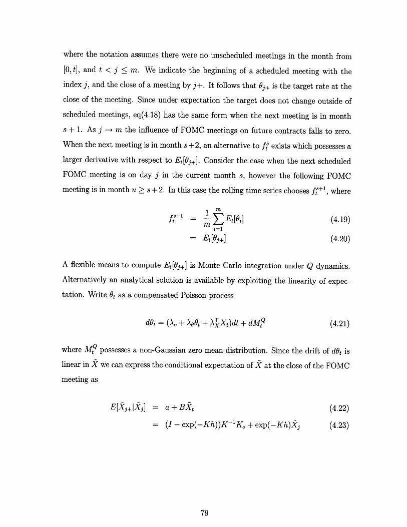
When the next meeting is in month s + 2, an alternative to f 9 exists which possesses a

larger derivative with respect to Et[9j+]. Consider the case when the next scheduled

FOMC meeting is on day j in the current month s, however the following FOMC

meeting is in month u 2 s + 2. In this case the rolling time series chooses fts+l, where

f -- = Et [O (4.19)i=1

=Et[Oj+] (4.20)

A flexible means to compute Et[Oj+] is Monte Carlo integration under Q dynamics.

Alternatively an analytical solution is available by exploiting the linearity of expec-

tation. Write Ot as a compensated Poisson process

dOt = (Ao + AoOe + ATXt)dt + dM Q (4.21)

where Mt possesses a non-Gaussian zero mean distribution. Since the drift of dOt is

linear in X we can express the conditional expectation of X at the close of the FOMC

meeting as

E[Xj+lX] = a + BXt (4.22)

= (I - exp(-Kh))K-1 Ko + exp(-Kh))Xj (4.23)

where j indicates the start of a meeting, j+ the close, h the length of a meeting, and

KO =

Ao

kQ01kQkg02

'v03

-Ao -A1

o kQ

0 kQ0 k31

(4.24)

-A2 -A 3

0 0

kQ k2

k3q kQ

(4.25)

To find E[X,jlXt] we again leverage the linearity of conditional expectation in affine

processes, and note Et[Oj] = Ot.

E[XjlXt] = c+DXt

= (I - exp(-K(j - t)))K-'Ko + exp(-K(j - t))Xt

where

k01Ko = k J

k03

kQK = kQ

k31

(4.26)

(4.27)

(4.28)

(4.29)

0 0

kQ2 kQ

Figure 4.2 shows the out-of-sample pricing errors of the constructed rolling time

series of Fed future contracts. The root means squared error over the sample is 5.090

bp. The model's ability to match Fed future contracts provides strong support to the

flexible jump dynamics. Since the future contracts are out-of-sample, this result also

provides substantial evidence that information in the yield market is also contained

in the Fed future market.

Error on Rolling Fed Future Contract: RMSE 5.090

10 .......

-15

fie%

-1998 1999 2000 2001 2002 2003 2004 2005 2006 20071998 1999 2000 2001 2002 2003 2004 2005 2006 2007

Figure 4-14: A time series ofcontracts.

out-of-sample pricing errors for near dated Fed Future

An alternative view of the model's ability to match information contained in

the Fed future contracts, is to invert the pricing relation to reveal jump intensities.

Specifically we invert eq(4.18) and eq(4.20) to expose the Fed future implied expected

change in the target at the next scheduled FOMC meeting. We can then easily

compare this time series to the equivalent metric in our model. Figure 4.2 plots the

two time series for comparison.

81

I i i I I I I I i

..... . . . . . . . ... . ........ ...... ......... .

...................! ... ... ... ... .. . . .. ... . . . . .. . . . . . . . . .

.......................................................

....... .. ...... ....... ....... .............I .......

. . .. . . . . . . . . ..

Model Expected Target Changes and Market Expected Jumps

:1II.. . . . . . . . .. . . .

I

. .. .. ... .

.. .... i ..... .... arko .I -o----- Market EO[Jump

-- Model E [Jumps

1998 1999 2000 2001 2002 2003 2004 2005 2006 2007

Figure 4-15: Time series of the number of 25 basis point jumps in the Fed target rateexpected to occur at the next scheduled FOMC meeting. Model EQ[Jumps] are takenfrom the model using the optimal model parameters of table 4.1. Market EQ[Jumps]are obtained by inverting the pricing relation for Fed future contracts.

82

0.5F

-0.5

-1.5

-2 . ...........

-2.5 ............

I I

' ' ' ' ' ;

:

...........

....... . ....

c

. . I

............

4.3 Yield Response to Shocks

Figure 4-16 plots the loadings of yields on the first three principle components (PC).

Since [46] first reported on the ability of three PCs to explain 99.95% of the variation

in yields, the literature has been referring to the three components as level, slope,

and curvature factors. Due to the shape of the curves in figure 4-16, we label PC1 as

the level factor, PC2 as the slope factor, and PC3 as the curvature factor.

Pricing Coefficients for Principle Components0.6 I

i: .... ...

0 .2 . ... .................... .. ........ .... .. . . .

-0 .2 . .. . . . . .. .... . .

-0 .4 ... ...... ..... .... ....... .... ....... .... . .... .. ...... ..... ...... ........... ........... ........

-0.6 . : Ci -

.PC2- -- -PC3

_ 0 II I I

0 1 2 3 4 5 6 7 8 9 10Maturity (yr)

Figure 4-16: Loadings for the first three Principle Components of Yields.

Figure 4-17 and 4-18 display normalized price loadings for model parameters given

in section 4.1. Specifically we plot normalized Cg of the pricing equation

Y(t, T) = Co(t, T) + Ck(t, T)(t + Et (4.30)

where C, = [Co, 1, C2, C3]. To view on the same scale we normalize each coefficient

to reflect the associated change in yields for a conditional one standard deviation

83

shock to Xt. Co is not normalized, thus it represents the yield response to a 1%

change in the target. We identify C2 as a curvature factor, as well as Co and C3 as a

slope factor. The remaining C2 is seen as a hybrid of the traditional factor labels. It

possesses traits of a slope factor at the mid to long end of the yield curve. However

near short to mid maturities is displays a strong curvature effect.

The meeting schedule of the FOMC injects the time variation found in Ck(t, T).

The only dynamics to change with the arrival of a scheduled meeting are the dynamics

associated with the target itself or d9t. However the coupling via the jump intensity

leads all state variables to display time variation, via the A coefficients of eq(3.22). It

follows that the time variation of Ck is greatest across a scheduled meeting. Figure

4-17 captures Cg directly before a meeting, while 4-18 plots C immediately after a

scheduled meeting. A convenient metric to view this seasonality is the days till the

next scheduled FOMC meeting. As this metric increases the influence of At and the

associated jumps in 0 have less of an effect on prices. Since X3 doesn't effect the jump

intensity of Ot, it possess a very small amount of time variation. For similar reasons

we find C2 to display the most time variation, which is supported by X 2 dominating

the jump intensity.

Monetary Policy Shocks

An active area of research is focused on identifying the response of asset prices to

shocks in monetary policy. We define shocks in monetary policy as unanticipated

changes in the Fed target rate. Since Fed future contracts are linked to the average

target rate over a single month, they serve as a natural choice to measure shocks

to the target rate. Our model construction provides a natural means to measure

monetary policy shocks and the resulting effect on yields.

Section 4.2 presents a rolling time series of Fed future contracts, which are con-

structed for maximum exposure to the next scheduled FOMC meeting. Model prices

of these contracts are formulated by computing the expected target change under

the pricing measure. Shocks however are measured under the historical P measure.

We define a shock to be the difference between the realized target change and the P

100

80

60

Normalized Pricing Vectors: Directly Before a FOMC Meeting

. . e+m Jump.-- -- +X1 Shock

I - - - -X2 Shock-I : : : . +X3 Shock

-200 1 2 3 4 5 6 7 8 9 10

Yield Maturity (yr)

Figure 4-17: Normalized pricing vector. Cx is normalized to display the response toa 1 standard deviation shock. Co requires no such normalization.

measurable expected change. The challenge in using Fed future contracts to extract

shocks is identifying the risk premium which distinguishes the two measures.

Recall the pricing relation for a time t Fed future contract given in section 4.2

fS 33fR = O + Et [+]m m(4.31)

where there are m days in month s, j indicates the start of the next scheduled FOMC

meeting, and j+ indicates the close of the meeting. It follows that Oj+ is the value

of the Fed target at the close of the meeting. To extract a shock we write eq(4.31)

85

i . , . ... . . . . . . . . ...

..........

... . . . . . . . . ...

................

. . . . .

100Normalized Pricing Vectors: Directly After a FOMC Meeting

-20' I I I I I0 1 2 3 4 5 6 7 8 9 10

Yield Maturity (yr)

Figure 4-18: Normalized pricing vector. Cx is normalized to display the response toa 1 standard deviation shock. Co requires no such normalization.

under P with an explicit risk premium.

= a, + E [9;+ +tm m

= O +j E[Aoj+] + lg

(4.32)

(4.33)

where p is the time t risk premium for the month s contract, and AOj+ is the target

change which occurred during the meeting. The expected change can now be written

as

m m= (f[ - Ot ) . 43tm- -3Et [AOj,+ (4.34)

The first term is the anticipated change we seek to measure, the second term is the

risk premium which corrupts the signal. The risk premium corruption is magnified

as j -- m. For completeness we give the associated monetary policy shock as

m mAj+ = m-j (fts - 9,) .- .P - A93+ (4.35)

m -3 m-j

where AO'+ denotes the unanticipated change in 0. An alternative method which

attempts to remove the risk premium of eq(4.35) is to measure the shock component

directly as first presented in [45].

If a change in the Fed target is fully anticipated, then the price of the associated

Fed future contract over the same period should remain constant. Assume the mar-

ket fully anticipates a 25 basis point increase at the next FOMC meeting which is

scheduled to occur tomorrow. Since the Fed future contracts are based on the future

expected average target rate, the 25 bp increase should be already priced in. It fol-

lows that any change in a Fed future contract across scheduled meetings represents

a revision in the expected target level for the remainder of the contract month. This

revision is a scaled measure of the monetary policy shock. Specifically we can define

monetary policy shocks as

AO.+ =- (f; - f;) (4.36)

where f] is the Fed future contract immediately before a scheduled meeting, fj+ is the

contract value immediately after the meeting, and s is the current month contract.

The critical assumption is the risk premium at time j is approximately equal to

the risk premium at time j+. Clearly a constant risk premium would satisfy this

assumption. Even if the risk premium is time varying, the variation should be small

over the course of one day.

Figure 4-19 plots monetary policy shocks derived from the model, as well as shocks

constructed via eq(4.36). We stress that the model calibration made no use of in-

formation in Fed future contracts. The two measures show an impressive overlap in

information content as measured by a 0.7632 sample correlation coefficient. The two

time series differ the most during the tightening cycle which began June 30th 2004.

During this period market participates widely expected the FOMC to raise the tar-

get by 25 basis at each consecutive meeting. This constant jump expectation poses

challenges to model dynamics.

Mearsures of Monetary Policy Shocks

: :

I I f'

. I

1998 2000

* I . A

*. I.. I .. ... ..........

- Model Shocks-. -- Empirical Shocks

2002 2004

Figure 4-19: Time seriesmeasured via Fed future

of model implied monetary policy shocks, as well as shockscontracts. Sample correlation of two measures is 0.7632.

Given measures of monetary policy shocks, we turn to the task of measuring the

effect of shocks on yields. We construct an empirical estimate of yield response to

policy shocks via a linear regression, and compare the results to the yield response

imbedded in our constructed model. We find the results to be almost identical.

To construct the effect of shocks on yields within the model framework, we look

88

20 .

10 ......

-10

-20 ......

-30 .....

An

1996 2006 2008

,v

to the model pricing formula.

Y(t, T) = Co(t, T) + Co(t, T)Ot + Cx(t, T)Xt + Et

Changes in yields are expressed as

Y(t + 1, T + 1)- Y(t, T)

where A04t+ 1 is the unanticipated change to the target at t + 1.

Co(t + 1, T + 1) defines how model yields respond to shocks.

For an empirical reference we follow [45] and fit weekly yields to

in the expected and unexpected changes in the target rate.

AYt = a + eAOt + ,lA0tO + Et

(4.38)

It follows that

a linear equation

(4.39)

where AO' is the expected target change and AO9 is the unexpected target change.

Most studies treat jump events separate from non-jump events, estimating eq(4.39)

from weekly samples where the target actually changed. The intuition typically being

that markets respond differently to these distinct events. We estimate the param-

eters of eq(4.39) via ordinary least squares (OLS). Table 4.7 reports the parameter

estimates using weekly data. The results are consistent with the results given in [45].

Figure 4-20 compares the model's ability to transmit monetary policy shocks to

yields. We find the model shows very close agreement with our empirical estimates.

(4.37)

= [Co(t + 1,T+1) - C(t,T)]

+ [Co(t + 1, T + 1)0t+1 + Co(t, T)Ot]

+ [Cx(t + 1, T + 1)Xt+1 - Cx(t, T)Xt]

S[Co(t + 1, T + 1) - Co(t, T)]

+ [Co(t + 1, T + 1)Et[0t+1] + Co(t, T)Ot]

+ [Cx(t + 1, T + 1)Xt+1 - Cx(t, T)Xt]

+ Co(t + 1, T + 1)AOut+ 1

Maturity (yr) a [ 1 J,, 1 R 2

0.5 0.53 11.62 98.76 0.75(0.8) (3.2) (7.6)

1 0.9 9.74 78.46 0.49(0.9) (1.9) (12)

2 0.89 6.33 58.74 0.23(0.7) (1) (6.9)

3 0.66 3.76 51.38 0.17(0.5) (0.6) (5.2)

4 0.41 2.73 45.98 0.13(0.3) (0.4) (4.2)

5 0.05 2.17 42.08 0.11(0.01) (0.3) (3.3)

6 -0.13 1.71 37.79 0.09(0.1) (0.3) (2.9)

7 -0.33 0.88 32.02 0.06(0.2) (0.1) (2.2)

8 -0.57 1.09 29.39 0.06(0.4) (0.2) (2)

9 -0.69 0.48 25.64 0.04(0.5) (0.1) (1.7)

10 -0.63 1.01 24.11 0.04(0.4) (0.1) (1.6)

Table 4.7: OLS estimates of the coefficients in eq(4.39). Heteroskedasticity-consistentWhite t-statistics in parentheses.

Yield response to a one percent shock to the Fed target rate

----- Model Coefficients---- OLS Coefficients

5 0 ........

4 0 .......... .......... .........

30

20

I I I I I I

0 1 2 3 4 5 6 7 8 9 10Maturity in Years

Figure 4-20: Response of Yields to shocks in monetary policy, as measured by unan-ticipated changes in the Fed target rate.

............ . . .. . . . .. . . . .

4.4 Risk Premium

A primary driver to conduct term structure research within a Dynamic Term Struc-

ture Model (DTSM) framework is the ability to easily identify risk premium. In this

section we focus on the model's ability to explain one year excess bond returns. We

find the inclusion of the Fed target as a state variable greatly improves the model's

predication of excess return. We find evidence that the improvement is due to the

target as a proxy for short dated rates. We also find substantial improvement when

the information embodied in the term structure of target rates is incorporated during

the estimation process. Thus the target also serves as a conduit to integrate market

participates expectations for future target levels. Linear regressions provide support

to the risk premium view of the target as a proxy for a short dated rate and a conduit

for the term structure of target rates.

Background

Define one year excess return on a n year bond as

xr(t + 1, n) = nY(t, n) - (n - 1)Y(t + 1, n - 1) - Y(t, 1) (4.40)

where Y(t, n) is the time t yield on an n year bond. Figure 4.4 plots the realized one

year excess return for our data set, using overlapping windows. In summary the one

year excess return is the return on a bond position above the one year yield available

at time t. The expectation hypothesis states that forward rates are rational expecta-

tions of future yields, and as such no time t information should predict excess bond

returns. In recent years several empirical studies have presented evidence rejecting

the expectation hypothesis by finding evidence of predictability in excess bond return.

There exists a rich set of literature which explores the predictability of bond

returns. One of the first studies [5] found the spread between forward rates and one

year yields predicted excess bond returns. [7] later showed the slope of current yield

increased this predictability. More recently a study in [14] showed that including all

1 Year Excess Return on {2,3,...,10) Bonds

-20'1997 1998 1999 2000 2001 2002 2003 2004 2005 2006

Figure 4-21: Realized one year excess return on {2, 3,..., 9, 10} year bonds usingweekly sampled bond yields. Return calculations use overlapping windows.

time t information in forward rates is important in explaining bond returns.2

We seek a model expression for the expected value of the return, or Et[xr(t + 1, n)].

Where we stress the expectation is under the historical P measure. Within a DTSM

framework we can express the three terms of eq(4.40) as

nY(t, n)

-(n - 1)E [Y(t + 1, n - 1)]

-Y(t, 1)

= -logE [exp (- tr(Xs)ds) (4.41)

= E [logE [exp ( t+ r(X,)ds) (4.42)

= logEt [exp (- j r(X,)ds) (4.43)

2[14] extend this to show a single factor, which is affine in yields, explains the majority of excessbond return.

Combine eq(4.41) and eq(4.43) to find

nY(t, n) - Y(t, 1)= -logEt exp (- f r(X)ds)] (4.44)

Cg(t + 1, n- 1)EtQ(t+) (4.45)

where we ignore terms related to the Jensen inequality. We remind readers that

though our state space is not affine, we presented a method to construct affine pricing

coefficients in section 3.2.4. A similar approximation for eq(4.42) results in

-(n- 1)E [Y(t + 1, n - 1)] C(t + 1, n - 1)E'P(.t+1 ) (4.46)

It follows that

E' [xr(t + 1, n)] C (t + 1, n - 1) [EP(kt+1) - EtQ (t+ 1) (4.47)

Eq(4.47) highlights how risk premium is specified and transmitted to bond returns.

The differences in drifts under each measure specifies the associated risk premium over

any period of time. The pricing coefficients Cg provide the weighting of each bond

to the risk premium. An alternative to using the approximation in eq(4.47) is to

compute the expected value of Y(t + 1, n - 1) via Monte Carlo and evaluate eq(4.40)

directly.

Model Performance

Using the model parameters of table 4.1 we evaluate eq(4.47) for overlapping one year

expected excess bond returns. Monte Carlo simulations confirm the errors induced by

ignoring the Jensen terms are well contained, and do not change the ensuing results.

The resulting model expected excess return is plotted in figure 4.4. We find the model

risk premium displays an ability to switch sign, due to the flexible specification of

section 3.2.3. Comparing the model expected excess return to the realized excess

return we find good tracking. With the exception of a window around 1999, the

model matches the level of risk premium quite well. In particular the model reflects

the negative dips in 2003 and 2005.

1 Year Expected Excess Return on {2,3,...,10} Bonds15

10

C3 5

x

0 0-(Dxa

-5 - -

-101997 1998 1999 2000 2001 2002 2003 2004 2005 2006

Figure 4-22: Model expected one year excess return on {2, 3,..., 9, 10} year bonds

using weekly sampled bond yields. Return calculations use overlapping windows.

To quantify the model's ability to reflect risk premium we use the coefficient of

determination or R 2. To better view the ensuing result we require a benchmark.

Since the purpose of our study is to investigate the effect of including the target in

an ATSM model we choose the A 1 (3) ATSM as a benchmark. As detailed in section

3.2.1 this is essentially our model without the target as a state variable. We calibrate

the model parameters using the same estimation method and weekly data set. A full

description of the model with estimated model parameters is available in Appendix

C.1.

Figure 4.4 plots the results. Ylds Only indicates the we are using the model pa-

rameters of table 4.1, which were estimated using the yield data. We note a significant

increase in performance with respect to the benchmark. We find a significant increase

in explanatory power up to the six year node, peaking at an additive five percent in

explained variation. The increase in performance begins to decline at the six year

node, converging to zero at ten years. The performance is consistent with many of our

previous findings and intuition. Figure 4-20 showed the response of yields to shocks

is strongest for shorted dated maturities. Figure 4-13 implies the strongest link to

monetary policy comes from the one and two year nodes. Section 4.3 detailed that

the dominating component of target jump intensity X 2 displays a curvature effect,

peaking at the two year node. These results are also in line with the discussion of the

target and it's role in adjusting the monetary base of section 1.

R2 Comparisons for 1 year Xret on n year yld:

--- Ylds Only-- *-- Benchmark

0 .6 .............

0 .5 5 ............ ............. ............

0.45 .

0.4 .

0.352 3 4 5 6 7 8 9 10

n year yld

Figure 4-23: Explaining excess bond returns. The Benchmark is a A1 (3) model withno jump component. Ylds indicates the use of model parameters of table 4.1, whichare estimated using yields only.

Term Structure of Target Rates

We are also interested in determining if information contained in the Fed future con-

tracts contain any risk premium information not already in yields. Recall section 4.2

presented small out-of-pricing errors for the rolling time series of Fed future contracts.

When the time series is incorporated during estimation the resulting pricing errors

are essentially unchanged, as are the other performance metrics discussed in section

4.1 and section 4.3. The associated R2 with respect to excess bond returns is also

relatively unchanged. Though there does seem to be a slight shifting of explanatory

power to the lower end of the yield curve.

Term Structure of Target Rates7.5

6 5.....

5.5-

401/04/00 01/07/00 01/10/00 01/01/01 01/04/01

Figure 4-24: Plot of the term structure of target rates taken from Fed future contractsduring the 2000 turning point. Doted line is the actual Fed target rate.

We now turn to the entire term structure of target rates. Define the term structure

of target rates to be the expected level of the target rate over the next the next twelve

months. This information is easily extracted from the currently traded Fed future

contracts. Figure 4.4 and 4.4 plot the full span of future contracts for two distinct

time periods. Each graphically demonstrates the additional information contact in

the additional contracts. We see in figure 4.4 that while the near dated contract is

essentially flat, the far dated contracts embed the market's believe of a turning point

in the target rate. In figure 4.4 we find the market belief that the Fed will tighten in

consistent but prolonged steps. It follows that the market's short term prediction of

the future target level may help predict excess return.

Term Structure of Target Rates

3 .5 .... ..... ... .... .... .... .... ..... .

2.5 3 -...........

2.5

1 .5 ...........

1'

01/07/04 01/10/04 01/01/05 01/04/05 01/07/05 01/10/05

Figure 4-25: Plot of the term structure of target rates taken from Fed future contractsduring the 2005 tightening cylce. Doted line is the actual Fed target rate.

We aim to include this information content by incorporating the long dated con-

tracts during the estimation process. Recall from section 4.2 that our model price for

a Fed future contract is the daily average value of the target rate during the contract

month. Fed future contracts trade for twelve months out, where open interest is of-

ten thin for later months. To avoid spurious contract prices, we remove any contract

.......... ...... *- ......

...........

who's open interest is less then ten percent of the total open interest. This normaliza-

tion ensures compensation for the six fold increase in total open interest since 2000.

Assume each contract possesses additive error identical to eq(4.11). Then the model

pricing equation for a Fed future contract for month s is

1Et[i] + Eti=1

(4.48)

where there are m days in month s. These contracts are priced in the model via the

techniques described in section 4.2.

R2 Comparisons for 1 year Xret on n year yld:

2 3 4 5 6n year yld

7 8 9 10

Figure 4-26: Explaining excess bond returns. The Benchmark is a A 1(3) model withno jump component. Ylds indicates the use of model parameters of table 4.1, whichare estimated using yields only. Ylds & Futures represents model performance whenyields and Fed future contracts are used to calibrate model parameters.

The resulting parameter estimates and in-sample pricing errors are in appendix

C.2. Comparing the errors in table C.3 to the errors of table 4.6, we conclude there is

Explaining 1 Year Xret via OLS0.7

0.65

0 .6 . .. .... ...

0.55 . . -E---) 3PC + FF rate

3PC + MM rate-*-- 3PC

0.452 3 4 5 6 7 8 9 10

Maturity, years

Figure 4-27: Explaining excess bond returns via ordinary lease squares regression.

3PC are the three principle components of all yields of section 3.4.2. MM indicates

the short dated 1 week money market rate. FF indicates the 1 month ahead Fed

Future contract as described in section 3.4.3.

no significant improvement to pricing errors when including the Fed future contracts.

However when we use the estimates of table C.2 to compute risk premium we find

substantial improvement. Figure 4-26 plots the associated R2 metrics for the three

cases we've discussed. For clarity we stress Ylds & Futures represents model perfor-

mance when yields and Fed future contracts are used to calibrate model parameters.

We find substantial improvement in the model's ability to predict excess bond return.

This result implies there is information in the term structure of Fed future contracts

which while it does not assist in pricing bonds, does help in predicting returns on

bonds. We stress that the future expected target changes imbedded in Fed futures is

under the pricing measure. We find the contracts especially at long dated intervals

display strong risk premium, which is supported by empirical studies [53].

100

Based on the above analysis we postulate that the improved predictability is due

to the target as a proxy for a short dated yield, and as a conduit for future expected

target changes. In an effort to support this view we turn to more empirical estimates

via linear regressions. Specifically we construct the first three principle components of

weekly yields, the one week money market rate, and a mid-dated Fed future contract.

We regress the realized excess return on this data and plot the associated R2 in figure

4.4. Comparing figure 4.4 to 4-26 we find many similarities. The relative spreads at

the short to mid maturities nodes displays excellent tracking. Unfortunately the long

dated maturities do not follow this trend. In summary figure 4.4 provides support to

the view that the improved predictability is due to the target as a proxy for a short

dated yield, and as a conduit for future expected target changes.

101

102

Chapter 5

Conclusion

This thesis investigated the implications of explicitly modeling the monetary policy

of the Central Bank within a Dynamic Term Structure Model (DTSM). We followed

Piazzesi (2005) and implemented monetary policy by including the Fed target rate as

a state variable. A non-linear switching process, was found to accurately model the

target dynamics while allowing for restrictions to ensure tractability. The flexible risk

specification of Cheridito et al (2007) was incorporated, with extensions to the target

jump process explored. Model parameters were estimated via a simulated maximum

likelihood estimation scheme with importance sampling. Finally a Bayesian particle

filter was found to be a useful robustness check.

Our results support those in Piazzesi (2005), revealing a substantial improvement

in pricing errors especially on the short end of the yield curve. The model construction

was shown to provide a natural framework to inspect monetary policy information

embedded in yields, which was found to be substantial. We found the addition of the

target rate improves the model's ability to explain excess return. An ability which

is increased with the inclusion of the full term structure of target rates, as measured

from Fed future contracts. We presented a view that the improved performance is due

to the target as a proxy for short term rates, and a conduit to express the information

content of the term structure of target rates.

103

104

Appendix A

Bond Pricing Accuracy Check

Two approximations were presented in section 3.2.4. The first concerned the non-

linear terms in the Feynman-Kac PDE of eq(3.22) which prevent the construction of

the ODEs, the essence of tractability in our problem. In section 3.2.4 we applied the

following Taylor Series expansion to achieve tractability.

A(X)I [B(t, T, X, 0 + sign(A(X))Jo) - B(t, T, )]

JoA(X)Co(t, T)B(t, T, X) (A.1)

The second concerned the normalization of scheduled FOMC meetings, by using the

true meeting grid for the first FOMC meeting and uniform spacing for all which

follow. The primary motivation for this approximation is computational efficiency.

However the meeting schedule for maturities over two years is never known to market

participates when prices are set. As such a normalization appears in line with market

realities.

We test both approximations simultaneously via a Monte Carlo estimation of bond

prices. We use the values of inferred state variables as initial conditions, and take

one draw by simulating the state space for ten years. Bond prices are then simple

Monte Carlo expectations. Table A.1 displays the results. MC-ODE is the RMSE of

the difference between the MC yields and the ODE yields.

105

Maturity (yr) Monte Carlo RMSE (bp) ODE RMSE (bp) MC-ODE (bp)

0.5 1.2076 0 1.20761 4.4001 4.3132 1.14042 1.2896 0 1.28963 2.0585 1.2804 1.41684 3.641 2.8824 1.4644

5 4.4284 3.6166 1.5333

6 4.6089 3.6875 1.66537 4.1519 3.0364 1.76378 3.4201 2.2263 1.85269 2.5737 0.99687 1.972710 2.0663 0 2.0663

Table A.1: Monte Carlo estimates of pricing errors due to linearization of the jumpterm and normalization of the meeting schedule. Root mean squared errors (RMSE)in basis points (pb). MC-ODE is the RMSE of the difference between the MC yields

and the ODE yields.

106

Appendix B

Estimation

B.1 Simulated Maximum Likelihood

Simulated Maximum Likelihood [49] is a popular method for estimation of continuous

time processes from discretely sampled data. Consider a continuous time drift diffu-

sion process X (t), who's dynamics are specified via the following stochastic differential

equation (SDE)

dX(t) = a(X(t), 7)dt + b(X(t), y)dW(t) (B.1)

where W is a standard Brownian Motion defined in a complete probability space, a

is a specified drift function, b is a specified diffusion function, and y ia a parameter

vector. Conditions on a, b, and y to ensure the existence and uniqueness are stated

in [49], and discussed at detail in [48].

Assume X is sampled at N+1 discrete points denoted as X(N) = (Xo, X 1, X 2,..., XN).

Assume a joint density fx (X(N); Y), with corresponding continuously differentiable

likelihood function Lx(X(N); ). Since X is a Markov process we write the likelihood

function as

Lx (X(N); ) = f(Xo; ) fx (Xn+l, tn+1IXn, tn, Y) (B.2)

In general the transition densities in the product are not known, and must be approxi-

mated. The SML method approximates the transition densities by simulating stochas-

tic paths between observations. Take the the transition density fx (Xn+1, tn+1 Xn, tn, _y)

107

as an example. Discretize time between tn and tn+1 into M subintervals of length h.

The transition density between these subintervals is then approximated as Gaussian.

The transition density for the first subinterval is

fx(x, tn+hIXn, tn, y) . q(x; Xn + ha(Xn, tn), hb(x, t,) 2 ) (B.3)

where 0(.; M, V) is the Gaussian density with mean M and variance V. The approxi-

mated transition density is then applied to subintervals up to the Mth - 1 subinterval.

At which point the approximation becomes

fx(X+1, tJn+1 X, Itn+1-h) e 0(Xn,1; X+ha(X, t,+l-h), hb(X-h, tn+l -h) 2) (B.4)

Where X is the simulated value at the indicated time. The estimate for the transition

density from tn to tn+1 is then taken via an average of eq(B.4). That is for J simulated

sample paths we find

1 Jfx(Xn+l , tn+llXn, tn) - (Xn+1 ; X + ha(X, tn+l - h), hb(X, tn+1 - h)2 ) (B.5)

j=1

The final expression in eq(B.5), can also be viewed as constructing the expectation of

a random variable z = fx (X+1, tn+1 z, t+ 1 - h), with a density drawn from simulated

paths and equal to fz(z, tn+1 -1 IX,, tn). Details on convergence of the SML estimator

to the true likelihood estimator is given in [49].

108

Appendix C

Details on Model Extensions

C.1 A1(3) Benchmark

In the language of [19] the benchmark model of section 4.4 is an A 1(3) model. This

is essentially the continuous component of the state space presented in section 3.2.1.

We leverage the same estimation scheme presented in 3.3, using the weekly data set

of section 3.4. We summarize here the model construction and estimation results.

The dynamics under P are given as

dXt = p (Xt)dt + a (Xt)dWtP

pP(Xt) = Ko ' + Xt = kP

k03

x -tla (Xt) = 0

0

0

V1 + b21XJt

0

0

kP2k32

(C.1)

0

kP2P3k33

.Xt

010

1 + b31X J

(C.2)

(C.3)

109

where

and

We employ the same flexible risk specification of section 3.2.3.

parametric form of dX under Q as

dXt = 1p(Xt)dt + o(Xt)dWt

This provides the

(C.4)

where

ko,

0

0

kQ

+ k21

k3

O 0kQ kQk22 k23

k3 k33

. Xt

We define the short rate as an affine function of the state space

r(Xt) = Po + plX 1 + P2X 2 + p3X 3

(C.5)

(C.6)

For admissibility we require

1. The two zeros in the first row of K P

2. k~, kQ > 0.5

01 01

3. b 1 > 0 forj= 1,2

For identification we require

1. The two zeros in Ko

2. pj > 0 for j = 2, 3

3. kQ2 > k33Q

To construct the A 1(3) pricing equations we substitute the above dynamics into

110

I-Q(xt) = K + KQ - X, =

the PDE of eq(2.6). The resulting system of ODEs is

dCo 1dt - o - CxlKol - 2 ( 2 + e ) (C.7)

dCxl 1dt - p1 + CxlK1l + Cx 2K 21 + CX3K31 - 2 (C21 + b21C0 2 + b31Ck3)(C.8)

dCX2 + CX2K 22 + CX3 K3 2 (C.9)dt

dCX3 3 + Cx 2K 23 + CX3K33 (C.10)dt

Since we no longer track the FOMC meeting schedule, the pricing equations are

time invariant, that is C(t, T) - C(n) for n = T - t. Table C.1 displays the point

estimates of the static model parameters. Unfortunately the small sample leads to

the vast majority of estimates being insignificant from zero at the 5% level.

C.2 Term Structure of Target Rates

Section 4.4 revealed that information embedded in the full term structure of target

rates improves the model's predictability of excess return. Where the term structure of

target rates are implied by the presently traded Fed future contracts. To incorporate

this information into the model, we assume each of the

Table C.2 contains the estimates of all model parameters, when all available Fed

future contracts priced. Table C.3 contains the associated in-sample pricing errors on

yields.

111

Parameter Estimate Standard Error t-Statistic

ko 2.6599 0.9772 2.7219kQ 0.6013 0.0070 85.7945

k2 698.8810 4840.9453 0.1444

k2 1.3683 0.0263 52.0106

k2 -2.3808 7.7402 -0.3076

kv -1.4796 12.6230 -0.1172

k( 0.0183 0.0594 0.3089

k( • le12 0.0001 0.0158 0.0000b21 30175.4829 412859.4780 0.0731bal 29118.9252 340783.4275 0.0854

Po 0.0892 0.0150 5.9397

Pi 0.0015 0.0002 6.2776

P2 0.0000 0.0001 0.1478

P3 * 1e9 0.2243 0.0000 0.0003ko 2.8781 111759.6540 0.0000k2 -0.0011 311.1590 0.0000k3P 0.0002 119.5947 0.0000kP 0.5517 8.3876 0.0658kP 741.5420 5173.3632 0.1433kP 1.1635 0.2849 4.0839

kP * le3 0.0139 0.5860 0.0000kP -0.0068 101.0657 -0.0001k2 -0.0003 0.1738 -0.0017kPf 0.3992 0.3730 1.0702

Table C.1: Point parameter estimates for the A 1(3) benchmark model. Estimates are

calculated via the simulated maximum likelihood technique described in section 3.3.1.

Sample period is from January 1997 to January 2007, including 521 weekly samples.

Standard errors are computed via the product of outer gradients [3].

112

Parameter Estimate Standard Error t-Statistic

kq 628.3403 3401.5785 0.1847

k 1.2650 0.0929 13.6216k2 0.2270 1.8885 0.1202

k2 1.6641 0.1129 14.7442

k2 -0.2510 7.3466 -0.0342

kc -0.0007 0.0220 -0.0309

kQ 0.0382 1.1084 0.0345

kQ 0.0001 0.0106 0.0113b21 0.0090 0.1898 0.0472b31 0.0314 2.0326 0.0155

Po -0.1203 0.3153 -0.3816

P1 0.0001 0.0002 0.3639

P2 * 1e6 0.0042 0.0000 0.0025

P3 0.0002 0.0068 0.0313Ao 2.7178 803.1086 0.0034AO -12404.1132 104.4304 -118.7788A1 4.6671 12.6287 0.3696

A2 201.5465 2044.9756 0.0986

A3 -0.0004 0.0690 -0.0056kP 2134.1209 11554.6181 0.1847koP -0.0133 215.3692 -0.0001k3 399.2485 13461.5025 0.0297kl 4.3172 0.9063 4.7633k2 0.0187 0.2171 0.0859kP 0.8700 0.4686 1.9766k2 -0.0027 0.4427 -0.0060k 1 0.1825 5.5741 0.0327kP 0.1272 3.8043 0.0334kf 0.7886 0.7130 1.1061

Table C.2: Point parameter estimates for the target model with information content

of the full term structure of target rates incorporated. Estimates are calculated via the

simulated maximum likelihood technique described in section 3.3.1. Sample period is

from January 1997 to January 2007, including 521 weekly samples. Standard errors

are computed via the product of outer gradients [3].

113

Maturity (yr) RMSE via map (bp) RMSE via Particle Filter (bp)0.5 0 3.71191.0 5.0916 3.34232.0 0 2.58933.0 3.3994 1.45114.0 4.7618 1.40195.0 4.8754 1.83116.0 4.2482 1.65107.0 3.3272 1.19598.0 2.3245 0.80599.0 1.2842 1.195510.0 0 2.0592

Table C.3: In sample pricing errors for the target model with information contentof the full term structure of target rates incorporated. RMSE via map is found byobserving the six month, two year, and ten year yields with no error and invertingthe measurement equation. RMSE via Particle Filter is obtained by applying theBayesian Particle Filter of section 3.3.2.

114

Bibliography

[1] Cbot fed funds futures. Chicago Board of Trade, 2003.

[2] M. S. Arulampalam, S. Maskell, N. Gordon, and T. Clapp. A tutorial on particlefilters for online nonlinear/non-gaussian bayesian tracking. IEEE Transactions

on Signal Processing, 50(No. 2), Feb. 2002.

[3] E. Berndt, B. Hall, R. Hall, and J. Hausman. Estimation and inference in

nonlinear structure models. Annals of Economic and Social Measurement, 3,1974.

[4] T. Bjork. Arbitrage Theory in Continuous Time, 2nd Edition.

[5] E. F. Bliss and R. R. Bliss. The information in long-maturity forward rates.American Economic Review, Vol. 77, 1987.

[6] Federal Reserve Board. Federal board of reserve of minneapolis.minneapolisfed. org/info/policy/dates-hist. cfm, 2006.

[7] J. Y. Campbell and R. J. Shiller. Yield spreads and interest rate movements: Abird's eye view. The Review of Economic Studies, Special Issue: The Economet-rics of Financial, Vol. 58, No. 3, 1991.

[8] 0. Cappe, E. Moulines, and T. Ryden. Inference in Hidden Markov Models.

Springer, New York, 2005.

[9] J. Carlson, J. McIntire, and J. Thomson. Fed funds futures as an indicator of

future monetary policy. Bederal Reserve Bank of Cleveland, Economic Commen-tary, November 2003.

[10] G. Chacko and S. Das. Pricing interest rate derivatives: A general approach.The Review of Financial Studies, Vol. 15(No. 1), Spring 2002.

[11] Z. Chen. Bayesian filtering: From kalman filters to particle filters, and beyond.Unpublished Manuscript McMaster Univeristy, 2003.

[12] P. Cheridito, D. Filipovic, and R.L. Kimmel. Market price of risk specificationsfor affine models: Theory and evidence. Journal of Financial Economics, 83(1),2007.

115

[13] S. V. Chernenko, K. B. Schwarz, and J. H. Wright. The information contentof forward and futures prices: Market expectations and the price of risk. Board

of Governors of the Federal Reserve System: International Finance DisscussionPapers, (8808), 2004.

[14] J. H. Cochrane and M. Piazzesi. Bond risk premia. American Economic Review,Vol. 95, 2005.

[15] R. Cont and P. Tankov. Financial Modelling with Jump Processes. Chapman &Hall/CRC, 2004.

[16] T. Cook and T. Hahn. The effect of changes in federal funds rate target onmarket interest rates in the 1970s. Journal of Monetary Economics, (Vol. 24),1989.

[17] J. C. Cox, J. E. Ingersoll, and S. A. Ross. A theory of the term structure ofinterset rates. Econometrica, Vol. 53(No. 2), March 1985.

[18] Q. Dai and K. Singleton. Term structure dynamics in theory and reality. TheReview of Financial Studies, Vol. 16(No. 3), 2003.

[19] Q. Dai and K. J. Singleton. Specification analysis of affine term structure models.The Journal of Finance, Vol. 55(No. 5), 2000.

[20] Q. Dai and K. J. Singleton. Expectation puzzles, time-varying risk premia, andaffine models of the term structure. Journal of Financial Economics, Vol. 63,2002.

[21] Datastream. Datastream: Data guide 9.0. DataStream User Guide Series, 2002.

[22] A. Doucet, N. de Freitas, and N. Gordon. Sequential Monte Carlo Methods inPractice. Springer-Verlag, New York, 2001.

[23] Jefferson Duarte. Evaluating an alternative risk preference in affine term struc-ture models. The Review of Financial Studies, 17(2), 2004.

[24] G. R. Duffee. Term premia and interest rate forecasts in affine models. TheJournal of Finance, Vol. 57, No. 1.

[25] D. Duffie. Dynamic Asset Pricing Theory. Princeton University Press, 2001.

[26] D. Duffie, D. Filipovic, and W. Schachermayer. Affine processes and applicationin finance.

[27] D. Duffie and R. Kan. Multi-factor term structure models. Philosophical Trans-actions: Physical Sciences and Engineering, Vol. 347(No. 1684), 1994.

[28] D. Duffie and R. Kan. A yield-factor model of interest rates. MathematicalFinance, 6, 1996.

116

[29] D. Duffie, J. Pan, and K. J. Singleton. Transform analysis and asset pricing foraffine jump-diffusions. Econometrica, Vol. 68(No. 6), Nov.

[30] G. Durham and A. R. Gallant. Numerical techniques for maximum likelihoodestimation of continuous-time diffusion processes. Journal of Business and Eco-nomic Statistics, 20(No. 3), July 2002.

[31] C. Edwards and G. Sinzdak. Open market operations in the1990s. Bederal Reserve Bank of New York, Economic Commentary,http://www.federalreserve.gov/pubs/bulletin/1997/1997111ead.pdf, 1997.

[32] 0. Elerian, C. Siddhartha, and N. Shephard. Likelihood inference for discretelyobserved nonlinear diffusions. Econometria, Vol. 69(No. 4), July 2001.

[33] M. J. Fleming and M. Piazzesi. Monetary policy tick-by-tick. Federal ReserveBank of New York, August 2005.

[34] M. J. Fleming and E. M Remolona. What moves the bond market? FederalReserve Bank of New York, Economic Policy Review, December, 1997.

[35] J. Geweke. Bayesian inference in econometric models using monte carlo integra-tion. Econometrica, 57(No. 6), Nov. 1989.

[36] M. Goodfriend and W. Whelpley. Federal Funds. Federal Reserve Bank of Rich-mond, 1993.

[37] N. Gordon, D. Salmond, and A.F.M Smith. Novel approach to nonlinear/non-gaussian bayesian state estimation. IEE Proceddings, 1993.

[38] M. Harrison and D. Kreps. Martingales and arbitrage in multiperiod securitiesmarkets. Journal of Economic Theory, 20, 1979.

[39] M. Harrison and S. Pliska. Martingales and stochastic integrals in the theory ofcontinuous trading. Stochastic Processes and Their Applications, 11, 1981.

[40] M. Heidari and L. Wu. Market anticipation of fed policy change sand the termstructure of interest rates. Working Paper, March 2006.

[41] J. James and N. Webber. Interest Rate Modelling: Financial Engineering. Wiley,2000.

[42] G. Jiang and S. Yan. Linear-quadratic term structure models - toward the un-derstanding of jump in interst rates. Journal of Banking & Finance, (10.1016),2008.

[43] M. Johannes. The statisitcal and economic role of jumps in continuous-timeinterest rate models. The Journal of Finance, Vol. LIX, No. 1, 2004.

[44] M. Johannes and N. Polson. MCMC Methods for Continuous-Time FinancialEconometrics. forthcoming.

117

[45] K. N. Kuttner. Monetary policy surprises and interest rates: Evidence from thefed funds futures market. Journal of Monetary Economics, 47, 2001.

[46] R. Litterman and J. Scheinkman. Common factors affecting bond returns. Jour-nal of Fixed Income, (54-61), 1991.

[47] J. Lund. Econometric analysis of continuous-time models of the term structureof interest rates. The Aarhus School of Business, Working Paper, 1994.

[48] B. Okensdal. Stochastic Differential Equations, Ed. 6. Springer-Verlag, Berlin-Heidelberg-New York, 2003.

[49] A. R. Pedersen. A new apporach to maximum likelihood estimation for stochasticdifferential equations based on discrete observations. Scand. J. Statistics, 1995.

[50] K. B. Petersen and V. Pozdnyakov. Predicting the fed. Univesity of Connecticut,Department of Economics, Working Paper, 2008.

[51] M. Piazzesi. Bond yields and the federal reserve. Journal of Political Economy,Vol. 113(No. 2), 2005.

[52] M. Piazzesi. Affine Term Structure Models. unpublished, 2006.

[53] M. Piazzesi and E. Swanson. Futures prices as risk-adjusted forecasts of monetarypolicy. National Bureau of Economic Research, (Working Paper 10547), 2004.

[54] M.K. Pitt and N. Shepard. Filtering via simulation: Auxiliary particle filters.Journal of the American Statistical Association, Vol. 94, 1999.

[55] C.P. Robert and G. Casella. Monte Carlo Statistical Methods, 2nd Edition.Springer, New York, 2004.

[56] W. J. Runggaldier. Jump-diffusions models. Universita di Padova, WorkingPaper, 2002.

[57] K. J. Singleton. Empirical Dynamic Asset Pricing. Princeton University Press,2006.

[58] K. J. Singleton. Empirical dynamic asset pricing :model specification and econo-

metric assessment. Princeton University Press, 2006.

[59] 0. Vasicek. An equilibrium characterization of the term structure. Journal of

Financial Economics, Vol. 5, 1977.

118


Recommended