Hindawi Publishing Corporation Mathematical Problems in Engineering Volume 2012, Article ID 937196, 17 pages doi:10.1155/2012/937196 Research Article A Fault Prognosis Strategy Based on Time-Delayed Digraph Model and Principal Component Analysis Ningyun Lu, 1 Bin Jiang, 1 Lei Wang, 1 Jianhua Lu, 2 and Xi Chen 3 1 College of Automation Engineering, Nanjing University of Aeronautics and Astronautics, Nanjing 210016, China 2 School of Computer Science and Engineering, Southeast University, Nanjing 210096, China 3 Department of Control Science and Engineering, Zhejiang University, Hangzhou 310027, China Correspondence should be addressed to Bin Jiang, [email protected]Received 30 August 2012; Accepted 15 November 2012 Academic Editor: Huaguang Zhang Copyright q 2012 Ningyun Lu et al. This is an open access article distributed under the Creative Commons Attribution License, which permits unrestricted use, distribution, and reproduction in any medium, provided the original work is properly cited. Because of the interlinking of process equipments in process industry, event information may prop- agate through the plant and affect a lot of downstream process variables. Specifying the causal- ity and estimating the time delays among process variables are critically important for data-driven fault prognosis. They are not only helpful to find the root cause when a plant-wide disturbance occurs, but to reveal the evolution of an abnormal event propagating through the plant. This paper concerns with the information flow directionality and time-delay estimation problems in process industry and presents an information synchronization technique to assist fault prognosis. Time- delayed mutual information TDMIis used for both causality analysis and time-delay estimation. To represent causality structure of high-dimensional process variables, a time-delayed signed digraph TD-SDGmodel is developed. Then, a general fault prognosis strategy is developed based on the TD-SDG model and principle component analysis PCA. The proposed method is applied to an air separation unit and has achieved satisfying results in predicting the frequently occurred “nitrogen-block” fault. 1. Introduction The desire and need for accurate diagnostic and real predictive prognostic capabilities are apparent in process industry. Detecting potential problems quickly and diagnosing them accurately before they become serious can significantly increase process safety, reduce production costs, and guarantee product quality. From the aspects of methodology and tech- nology, it involves fault detection, fault diagnosis, and fault prognosis the three major tasks of prognostics and health management PHMsystems. Fault prognosis is the most difficult one, since it requires the ability to acquire knowledge about events before they actually
Transcript
Hindawi Publishing CorporationMathematical Problems in EngineeringVolume 2012, Article ID 937196, 17 pagesdoi:10.1155/2012/937196
Research ArticleA Fault Prognosis Strategy Based on Time-DelayedDigraph Model and Principal Component Analysis
Ningyun Lu,1 Bin Jiang,1 Lei Wang,1 Jianhua Lu,2 and Xi Chen3
1 College of Automation Engineering, Nanjing University of Aeronautics and Astronautics,Nanjing 210016, China
2 School of Computer Science and Engineering, Southeast University, Nanjing 210096, China3 Department of Control Science and Engineering, Zhejiang University, Hangzhou 310027, China
Received 30 August 2012; Accepted 15 November 2012
Academic Editor: Huaguang Zhang
Copyright q 2012 Ningyun Lu et al. This is an open access article distributed under the CreativeCommons Attribution License, which permits unrestricted use, distribution, and reproduction inany medium, provided the original work is properly cited.
Because of the interlinking of process equipments in process industry, event informationmay prop-agate through the plant and affect a lot of downstream process variables. Specifying the causal-ity and estimating the time delays among process variables are critically important for data-drivenfault prognosis. They are not only helpful to find the root cause when a plant-wide disturbanceoccurs, but to reveal the evolution of an abnormal event propagating through the plant. This paperconcerns with the information flow directionality and time-delay estimation problems in processindustry and presents an information synchronization technique to assist fault prognosis. Time-delayed mutual information (TDMI) is used for both causality analysis and time-delay estimation.To represent causality structure of high-dimensional process variables, a time-delayed signeddigraph (TD-SDG) model is developed. Then, a general fault prognosis strategy is developedbased on the TD-SDG model and principle component analysis (PCA). The proposed method isapplied to an air separation unit and has achieved satisfying results in predicting the frequentlyoccurred “nitrogen-block” fault.
1. Introduction
The desire and need for accurate diagnostic and real predictive prognostic capabilitiesare apparent in process industry. Detecting potential problems quickly and diagnosingthem accurately before they become serious can significantly increase process safety, reduceproduction costs, and guarantee product quality. From the aspects of methodology and tech-nology, it involves fault detection, fault diagnosis, and fault prognosis (the three major tasksof prognostics and health management (PHM) systems). Fault prognosis is the most difficultone, since it requires the ability to acquire knowledge about events before they actually
2 Mathematical Problems in Engineering
occur [1]. There has been much more progress made in fault detection and diagnosis than inprognosis [2–5]. Despite the difficulties, some impressive achievements have been made infault prognosis, which has been approached via a variety of techniques, including model-based methods such as time-series prediction, Kalman filtering, and physics or empirical-based methods; probabilistic/statistical methods such as Bayesian estimation, the Weibullmodel; data-driven prediction techniques such as neural network. References [1, 4, 5] hadgiven comprehensive surveys on those fault prognosis methods.
For process industry, quantitatively data-driven methods are more attractive, becauseaccurate analytical models are usually unavailable due to process complexity, while abundantprocess measurements can provide a wealth of information upon process safety and productquality. For almost all data-based process modeling, monitoring, fault detection, diagnosis,or prognosis methods, process measurements collected by the distributed control systems(DCS) adopted in many industrial plants are synchronized by sampling time. But in manyindustrial processes, such as oil refining, petrochemicals, water and sewage treatment, foodprocessing, and pharmaceutical, raw materials are processed sequentially by a series ofinterlinked units along the production line. Flowing material generates flowing information.Synchronizing process measurements by sampling time implies that information delay mayexist among correlated process variables located in different operation units.
For convenience, a process with two units A and B is considered, where xA and xB aretwo correlated variables measured at each unit, and the production material flows from A toB, as shown in Figure 1.
Suppose that an abnormal event is occurring in unit A at time k and it is not serious tocause any alarming in unit A, the event will appear in unit B at time k + τ , where τ is thetime-delay determined by process characteristics. Process measurement xA(k) may beaffected by the event immediately, but xB(k) is still in normal state until at time k + τ . Theearly-stage event information may be obscured by the downstream measurements if we treatprocess measurements in the routine form {xA(k), xB(k)} instead of the time-series form{xA(k), xB(k + τ)}. Synchronizing process measurements by event information instead ofsampling time can highlight the early-stage process abnormalities, which is of importance forrealizing earlier fault detection and diagnosis for industrial processes.
Information synchronization has received extensive attentions in many scientific fieldssuch as physics, medicine and biology, computer science, or even economy and ergonomics[6, 7]. Causality (i.e., the cause-effect relationship or dynamical dependence) can be detectedby synchronizing the temporal evolutions of two coupled systems [8]. It is apparent that,it will be easier to carry out fault prognosis in an industrial process when the dynamicalinterdependences among process variables are retrieved.
In order to realize information synchronization and further benefit fault prognosis, twobasic issues, identification of causality and estimation of time-delay among variables wheninformation flow goes through the subsystems, must be firstly solved. Specifying the causal-ity and estimating the time-delays among process variables are critically important for data-driven fault prognosis in process industry. They are not only helpful to find the root causewhen a plant-wide disturbance occurs in a complex industrial process, but to reveal the evolu-tion of an abnormal event propagating through the plant.
There is an extensive literature on causalitymodeling, applying, and combiningmathe-matical logic, graph theory, Markov models, Bayesian probability, and so forth [10]. Recently,information-theoretic approaches arouse more attention, where causality can be quantifiedand measured computationally. The linear framework for measuring and testing causalitywas developed by Granger who proposed the definition of Granger causality (GC) and two
Mathematical Problems in Engineering 3
τ
A BMaterials Product
xA(k − 1)
xA(k)
xA(k + 1)
xB(k − 1)xB(k)
xB(k + 1)
Process measurements {xA(k), xB(k)}
Figure 1: Illustration of information flow in process industry.
well-known test statistics, the Granger-Sargent test and the Granger-Wald test [11, 12]. Thenonlinear extensions of the Granger causality based on the information-theoretic formulationwere also reported [13], such as transfer entropy [14] and conditional mutual information[15]. It has been proven that, with proper conditioning, transfer entropy is equivalent toconditional mutual information. In the field of neurophysiology, in order to designate thedirection of information flow, time-delayed mutual information (TDMI) has been introducedto measure causal interactions in event related functional Magnetic Resonance Imaging(fMRI), electroencephalograph (EEG), and Magnetoencephalograph (MEG) experiments[16, 17]. TDMI has a very similar theoretic background with transfer entropy or conditionalmutual information, but the relationship among the three methods is not yet completelyproven.
In causal analysis of two variables in industrial process, time-delay estimation natu-rally arises. Because of the interlinking of process equipments, event information may prop-agate through the plant and affect a lot of downstream process variables. If information flowdirection can be determined, then a time-delayed correlation can be taken as evidence ofcausality due to physical causation. There are several methods published in literatures thatcould be used to determine the time-delay. A practical method was proposed that used cross-correlation function to estimate the time-delay between process measurements and derivedcausal maps for identifying the propagation path of plant-wide disturbances [18]. Cross-cor-relation technique has the benefits of simple concept and fast computation. However, itrequires the correlations between measurements to be linear. Automutual information (AMI)was also adopted to deal with time-delay in a single time series [19], which can be extendedto multivariate time series. Compared to cross-correlation technique, entropy-based methodssuch as AMI or TDMI are more general as they can deal with nonlinear correlations.
This paper concerns with the information flow directionality and time-delay estima-tion problems in process industry and presents an information synchronization technique toassist fault prognosis. TDMI will be used in this paper as it can be easily modified for bothcausality detection and time-delay estimation. To represent causality structure of high-dimen-sional process variables, a time-delayed signed digraph (TD-SDG) is then developed as aprocess model. Then, a general fault prognosis strategy is developed, which consists of twophases: offline modeling (phase I) and online fault prognosis (phase II). In phase I, processmeasurements collected from historical database are rearranged into time series form. Awidely used statistical projection method, principle component analysis (PCA), is used fordatamodeling. Data-based predictionmodels should also be developed offline for all nonroot
4 Mathematical Problems in Engineering
nodes in the TD-SDG process model, because in phase II, the first thing is to predict the futureprocess measurements to arrange process data in time-series form for online informationsynchronization.
The proposed fault prognosis strategy is applied to an air separation unit (ASU). TheASU suffers from frequent nitrogen-blockage fault in the argon production subsystem. Theapplication results show that, it can achieve early and accurate detection of the nitrogen-blockage fault and meet the application needs.
2. An Information Synchronization Technology
2.1. Information’s Directionality and Time-Delay Estimation
Entropy (or information entropy) is the most popular measure for quantifying informationin random variable. To quantify the dependency for bi- or multivariate random variables,mutual information is widely used. Let us consider two time series X and Y . Each time seriescan be thought of as a random variable with underlying probability density function (PDF),p(x) or p(y). The mutual information (MI) between X and Y is defined as
MI(X,Y ) =∑
x∈X
∑
y∈Yp(x, y
)log
(p(x, y
)
p(x)p(y)), (2.1)
where p(x, y) is the joint PDF between X and Y .The mutual information function is strictly nonnegative and has a maximum value
when the two variables are completely identical. Note that MI(X,Y ) is symmetric under theexchange of X and Y , and therefore it quantifies the amount of dependency but cannotmeasure its directionality or causality. However, it is easy to obtain asymmetric MI, calledtime-delayed mutual information (TDMI), by adding a time-delay (τ) in one of the variablesusing the following equations:
TDMIXY (τ) =∑
i,j
p(xi, yj+τ
)log
p(xi, yj+τ
)
p(xi)p(yj+τ
) ,
TDMIYX(τ) =∑
i,j
p(yj, xi+τ
)log
p(yj , xi+τ
)
p(yj
)p(xi+τ)
.
(2.2)
TDMI was firstly suggested by Fraser and Swinney [20] as a tool to determine a rea-sonable delay between two series. If the time-delayed mutual information exhibits a markedminimum at a certain value of τ∗, then this is a good candidate for a reasonable time-delay. Inthe field of neurophysiology [21], TDMIwas extended to indicate the direction of informationflow. Since TDMIXY and TDMIYX are not symmetric, the difference between them, NIXY =TDMIXY − TDMIYX , can show the net flux of information, which may be interpreted as theinformation flow between them. If NIXY is positive, then the information flows from X to Yand vice versa [21].
This idea is very similar with transfer entropy, but it is more attractive because of thefollowing reason. Although transfer entropy is effective in determining the directionality andit has been applied to specify the directionality of fault propagation path in some industrial
Mathematical Problems in Engineering 5
processes according to the literatures [22, 23], it is difficult to determine the time-delaycompared with the TDMI-based method according to our experiments. Back to the motiva-tion of synchronizing process measurements in terms of event information, time-delay is ofthe same importance as information directionality. Therefore, a TDMI-based causalityanalysis and time-delay estimation method is proposed as below.
According to [20], the TDMImethod estimates the time-delay τ∗ when the TDMI func-tion shows the first local optimum. By (2.2), the time-delays τ∗XY and τ∗YX can be defined as
τ∗XY = Maxτ →N
{TDMIXY (τ)},
τ∗YX = Maxτ →N
{TDMIYX(τ)},(2.3)
where N is the length of the estimation window. To specify information directionality, anindex is introduced as
DXY = TDMIXY
(τ∗XY
) − TDMIYX(τ∗YX
). (2.4)
If DXY is positive, then the information flows from X to Y with the time-delay τ∗XY ; if DXY isnegative, then the information flows from Y to X with the time-delay τ∗YX .
Compared to the method in [21], the above method can estimate informationdirectionality and time-delay simultaneously.
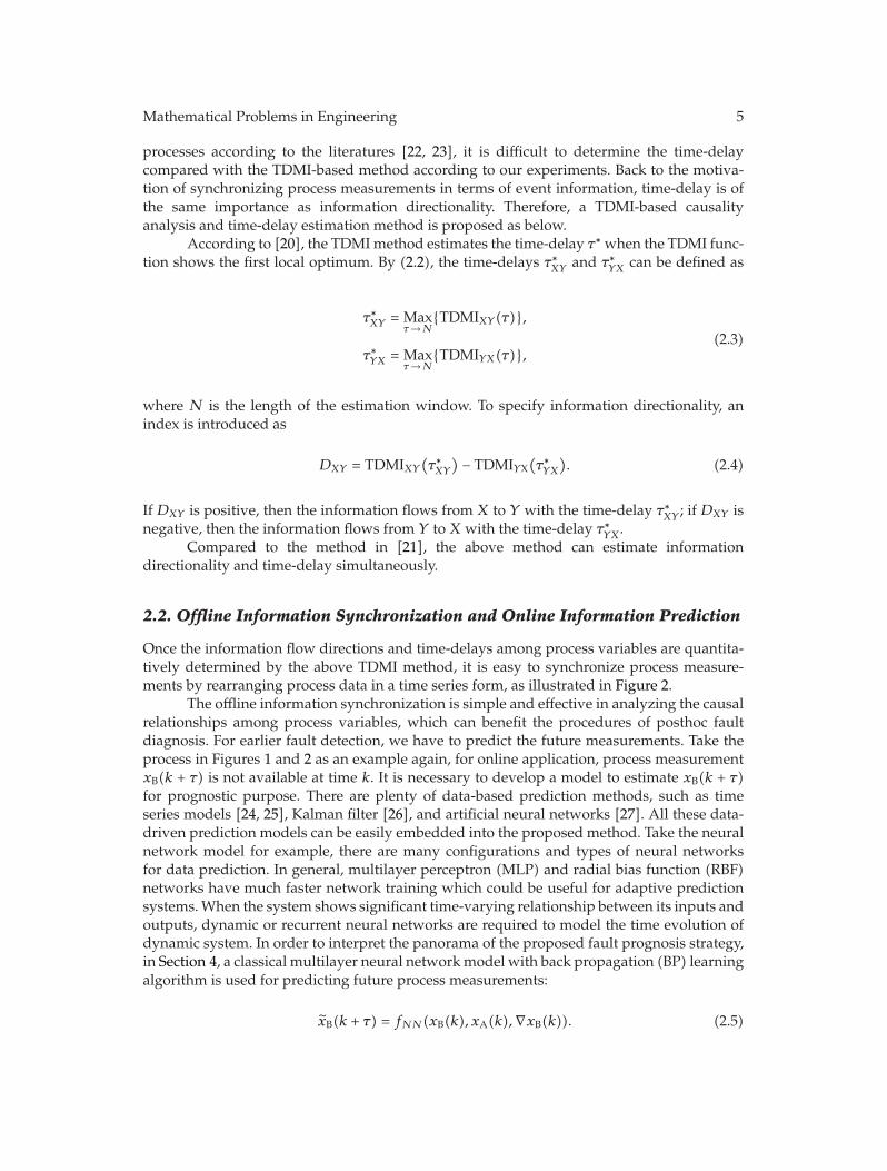
2.2. Offline Information Synchronization and Online Information Prediction
Once the information flow directions and time-delays among process variables are quantita-tively determined by the above TDMI method, it is easy to synchronize process measure-ments by rearranging process data in a time series form, as illustrated in Figure 2.
The offline information synchronization is simple and effective in analyzing the causalrelationships among process variables, which can benefit the procedures of posthoc faultdiagnosis. For earlier fault detection, we have to predict the future measurements. Take theprocess in Figures 1 and 2 as an example again, for online application, process measurementxB(k + τ) is not available at time k. It is necessary to develop a model to estimate xB(k + τ)for prognostic purpose. There are plenty of data-based prediction methods, such as timeseries models [24, 25], Kalman filter [26], and artificial neural networks [27]. All these data-driven prediction models can be easily embedded into the proposed method. Take the neuralnetwork model for example, there are many configurations and types of neural networksfor data prediction. In general, multilayer perceptron (MLP) and radial bias function (RBF)networks have much faster network training which could be useful for adaptive predictionsystems.When the system shows significant time-varying relationship between its inputs andoutputs, dynamic or recurrent neural networks are required to model the time evolution ofdynamic system. In order to interpret the panorama of the proposed fault prognosis strategy,in Section 4, a classical multilayer neural networkmodel with back propagation (BP) learningalgorithm is used for predicting future process measurements:
xB(k + τ) = fNN(xB(k), xA(k),∇xB(k)). (2.5)
6 Mathematical Problems in Engineering
A B A B
Routine form Time series form
A B
·········
······
······Date re-arrangement
τxA(k − 1)
xA
xA(k + 1)
xA(k − 1)
xA
xA(k + 1)
xB(k − 1)
xB
xB(k + 1)
{xA(k), xB(k)} {xA(k), xB(k + τ)}
xB(k + τ − 1)
xB(k + τ)
xB(k + τ + 1)
Figure 2: Rearrangement of process data for the illustrative process in Figure 1.
x1 x2
x3
x4 x5
{MI1,2, τ1,2} {MI2,4, τ2,4} MI4,5, τ4,5{ }
{MI1,3, τ1,3} {MI3,4, τ3,4}
{MI 2,3, 0}
{MI2,5, τ2,5}
Figure 3: Illustration of the developed SDG model.
That is, xB(k + τ) is estimated based on the available measurements {xA(k), xB(k)} and thetrend term ∇xB(k) at time k.
2.3. Time-Delayed SDG Process Model
In Section 2.1, a pair-wise causality detection and time-delay estimation method is given fortwo random process variables. To deal with the high dimensionality of an industrial process,it is better to develop a signed digraph (SDG)model to represent the causality structure.
In a standard SDG model, nodes correspond to process variables; arcs represent theimmediate influence between the nodes. Positive or negative influence is distinguished bythe sign (+) or (−), assigned to the arc. In the SDG developed here, called time-delayed SDGmodel (TD-SDG), the arcs will be assigned to represent the time-delayedmutual information,{MIi,j , τi,j}; the arrows on the arcs indicate the directionality of information flow. The solidarcs represent positive correlation, while dashed arcs represent negative correlation. Figure 3gives an illustrative example of a TD-SDG model.
The above TD-SDGmodel can be derived quantitatively from historical data followingthe work of [18]. Process topology will be extracted automatically based on the causalitymatrix. Consistency check is necessary to ensure the correctness of the derived TD-SDGmodel. In addition, since the proposed entropy-based information synchronization is statis-tical, significance testing and threshold settings are also necessary. The major steps fordeveloping the TD-SDG model are summarized in Figure 4.
Mathematical Problems in Engineering 7
Step 1: select process variables and do data pretreatment.
Step 2: pair-wisely calculate TDMI to determine the directions
and time delays.
Step 3: obtain the causality matrix.0
0
0
Step 4: simplify the causality matrix.
Step 5: construct causality map.
Step 6: construct TD-SDG model.
DXY = TDMIXY (τ∗XY ) − TDMIYX(τ∗YX).
x1 x2
x3
x4 x5
x1
x2
x3
x4
x5
D′ =
D =
x1 x2 x3 x4 x5
0
0
0
0 00 0
00 0
0
0
0
0
0
001 1
01
01
1
e
x1 x2
x3
x4 x5
{ IM 1,2, τ1,2} {MI2,4, τ2,4}
MI4,5, τ4,5{ }
{MI1,3, τ1,3} {MI3,4, τ3,4}
{MI2,3, 0}
{MI2,5, τ2,5}
.
.D2,1
D1,2
Dm,1 Dm,2
D1,m
D2,m
·········
· · ·
· · ·· · ·
· · ·
Figure 4: Key steps in constructing the TD-SDG model.
8 Mathematical Problems in Engineering
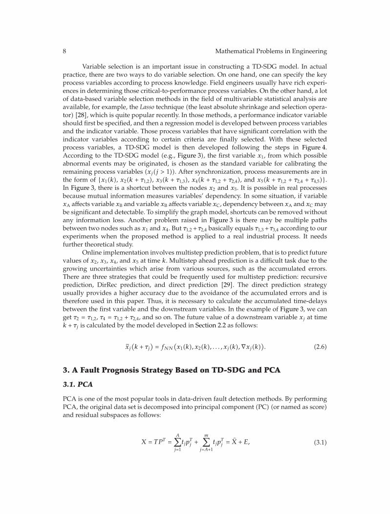
Variable selection is an important issue in constructing a TD-SDG model. In actualpractice, there are two ways to do variable selection. On one hand, one can specify the keyprocess variables according to process knowledge. Field engineers usually have rich experi-ences in determining those critical-to-performance process variables. On the other hand, a lotof data-based variable selection methods in the field of multivariable statistical analysis areavailable, for example, the Lasso technique (the least absolute shrinkage and selection opera-tor) [28], which is quite popular recently. In those methods, a performance indicator variableshould first be specified, and then a regression model is developed between process variablesand the indicator variable. Those process variables that have significant correlation with theindicator variables according to certain criteria are finally selected. With these selectedprocess variables, a TD-SDG model is then developed following the steps in Figure 4.According to the TD-SDG model (e.g., Figure 3), the first variable x1, from which possibleabnormal events may be originated, is chosen as the standard variable for calibrating theremaining process variables (xj(j > 1)). After synchronization, process measurements are inthe form of {x1(k), x2(k + τ1,2), x3(k + τ1,3), x4(k + τ1,2 + τ2,4), and x5(k + τ1,2 + τ2,4 + τ4,5)}.In Figure 3, there is a shortcut between the nodes x2 and x5. It is possible in real processesbecause mutual information measures variables’ dependency. In some situation, if variablexA affects variable xB and variable xB affects variable xC, dependency between xA and xC maybe significant and detectable. To simplify the graph model, shortcuts can be removed withoutany information loss. Another problem raised in Figure 3 is there may be multiple pathsbetween two nodes such as x1 and x4. But τ1,2 + τ2,4 basically equals τ1,3 + τ3,4 according to ourexperiments when the proposed method is applied to a real industrial process. It needsfurther theoretical study.
Online implementation involves multistep prediction problem, that is to predict futurevalues of x2, x3, x4, and x5 at time k. Multistep ahead prediction is a difficult task due to thegrowing uncertainties which arise from various sources, such as the accumulated errors.There are three strategies that could be frequently used for multistep prediction: recursiveprediction, DirRec prediction, and direct prediction [29]. The direct prediction strategyusually provides a higher accuracy due to the avoidance of the accumulated errors and istherefore used in this paper. Thus, it is necessary to calculate the accumulated time-delaysbetween the first variable and the downstream variables. In the example of Figure 3, we canget τ2 = τ1,2, τ4 = τ1,2 + τ2,4, and so on. The future value of a downstream variable xj at timek + τj is calculated by the model developed in Section 2.2 as follows:
xj
(k + τj
)= fNN
(x1(k), x2(k), . . . , xj(k),∇xj(k)
). (2.6)
3. A Fault Prognosis Strategy Based on TD-SDG and PCA
3.1. PCA
PCA is one of the most popular tools in data-driven fault detection methods. By performingPCA, the original data set is decomposed into principal component (PC) (or named as score)and residual subspaces as follows:
X = TPT =A∑
j=1
tjpTj +
m∑
j=A+1
tjpTj = X + E, (3.1)
Mathematical Problems in Engineering 9
where Xn×m is the data matrix, n is the number of samples, m is the number of process var-iables, A is the number of PCs retained in score subspace, tj is the score vector, pj is the load-ing vector by which the original variables are projected into score subspace, T and P are scorematrix and loading matrix, respectively, X is the reconstructed data matrix, X = XPAP
TA, PA
consists of the first A columns of the loading matrix P , and E is the residual matrix.For process data, x(k) = [x1(k), . . . , xm(k)], the Hotelling’s T2 and the squared predic-
tion error (SPE) statistics are calculated in the score and residual subspaces, respectively,
T2 = tΛ−1tT ,
SPE = eeT = (x − x)(x − x)T ,(3.2)
where t1×A is the score vector for the data sample x(k), x(k) is the reconstruction of x(k), Λis the diagonal matrix consisting of the eigenvalues of covariance matrix XTX. SPE gives ameasure of the distance of an observation from the space defined by the PCA model, whileT2 measures the shift of an observation in the mean of the scores. For process monitoringand fault detection, SPE is the main criterion of process abnormality. But in some exceptionalsituations where the fault does not alter the correlation structure of process variables, T2 willbe used to assist fault detection. The control limits of SPE and T2 can be calculated from thenormal values with certain statistical assumptions. If any of the two statistics is beyond thecontrol limit, then it means the measurements cannot be described by the PCAmodel, and anabnormality may happen [30].
3.2. PCA-Based Fault Prognosis
PCA is performed on the synchronized process data as follows:
X = T P T , (3.3)
where X = [x1, x2, . . . , xm], xj(j = 2, . . . , m) are the variables after information synchroniza-tion. In the modeling phase or in the offline analysis, and xj(j = 2, . . . , m) can be the trueprocess measurements. For online application, future measurements xj(k + τj)(j = 2, . . . , m)can be obtained by the neural network prediction model given by (2.6).
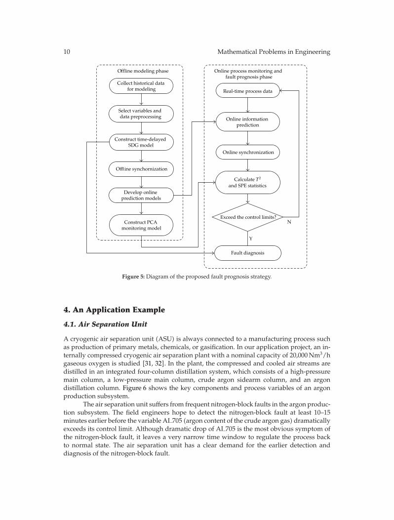
Once online synchronized data x(k) = [x1(k), x2(k + τ1), . . . , xm(k + τm)] is obtained,SPE can be calculated by the PCA model for online fault detection. The proposed faultprognosis strategy can be summarized by Figure 5, which contains the key steps in offlinemodeling phase (phase I) and online process monitoring and fault prognosis phase (phaseII).
It should be noted that, PCA is only applicable to stationary processes. For nonsta-tionary processes, independent component analysis (ICA) can be used as a fault detectiontool instead of the PCA method in the proposed fault prognosis strategy.
10 Mathematical Problems in Engineering
Offline modeling phase
Collect historical data for modeling
Select variables and data preprocessing
Construct time-delayed SDG model
Offl ine synchornization
Develop online prediction models
Construct PCA monitoring model
Online process monitoring and fault prognosis phase
Real-time process data
Online information prediction
Online synchronization
Calculate T2
and SPE statistics
Exceed the control limits?
Fault diagnosis
Y
N
Figure 5: Diagram of the proposed fault prognosis strategy.
4. An Application Example
4.1. Air Separation Unit
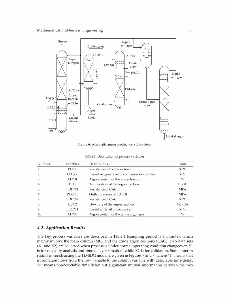
A cryogenic air separation unit (ASU) is always connected to a manufacturing process suchas production of primary metals, chemicals, or gasification. In our application project, an in-ternally compressed cryogenic air separation plant with a nominal capacity of 20,000Nm3/hgaseous oxygen is studied [31, 32]. In the plant, the compressed and cooled air streams aredistilled in an integrated four-column distillation system, which consists of a high-pressuremain column, a low-pressure main column, crude argon sidearm column, and an argondistillation column. Figure 6 shows the key components and process variables of an argonproduction subsystem.
The air separation unit suffers from frequent nitrogen-block faults in the argon produc-tion subsystem. The field engineers hope to detect the nitrogen-block fault at least 10–15minutes earlier before the variable AI 705 (argon content of the crude argon gas) dramaticallyexceeds its control limit. Although dramatic drop of AI 705 is the most obvious symptom ofthe nitrogen-block fault, it leaves a very narrow time window to regulate the process backto normal state. The air separation unit has a clear demand for the earlier detection anddiagnosis of the nitrogen-block fault.
Mathematical Problems in Engineering 11
PAC
Nitrogen
Crude argon
FI 702
LIC 701
Liquid nitrogen
CAC I
CAC II
PDI
701
Liquid nitrogen
Liquid nitrogen
Crude argon
Argon fraction
liquid
Air
OxygenArgon fraction
TI 16
AI 701
Crude argon
PDI 702
PIS 701
AI 705
Liquid nitrogen
Liquied argon
Crude liquid argon
LIAS 2
PDI 1
Figure 6: Schematic argon production sub-system.
Table 1: Description of process variables.
Number Variables Descriptions Units
1 PDI 1 Resistance of the lower tower KPA2 LIAS 2 Liquid oxygen level of condenser evaporator MM3 AI 701 Argon content of the argon fraction %4 TI 16 Temperature of the argon fraction DEGC5 PDI 701 Resistance of CAC I MPA6 PIS 701 Outlet pressure of CAC II MPA7 PDI 702 Resistance of CAC II KPA8 FI 702 Flow rate of the argon fraction M3/HR9 LIC 701 Liquid air level of condenser MM10 AI 705 Argon content of the crude argon gas %
4.2. Application Results
The key process variables are described in Table 1 (sampling period is 1 minute), whichmainly involve the main column (MC) and the crude argon columns (CAC). Two data sets(X1 and X2) are collected when process is under normal operating condition changeover. X1is for causality analysis and time-delay estimation, while X2 is for validation. Some interimresults in constructing the TD-SDGmodel are given in Figures 7 and 8, where “1” means thatinformation flows from the row variable to the column variable with detectable time-delay;“e” means nondetectable time-delay but significant mutual information between the two
12 Mathematical Problems in Engineering
1111
111111111
11111 111
11111111
11111111
1111
10
PDI 1LIAS 2AI 107
TI 16PDI 701PIS 701PDI 702
FI 702LIC 701
AI 705
e
——
——
——e
e——
——
PDI 1 LIAS 2 AI 107 TI 16 PDI 701 PIS 701 PDI 702 FI 702 LIC 701 AI 705
Figure 7: The causality matrix for ASU process.
11
1
1 1
111111
11
1
0
0
PDI 1LIAS 2AI 107
TI 16PDI 701PIS 701PDI 702
FI 702LIC 701
AI 705
e
——
——
——e
e——
——
PDI 1 LIAS 2 AI 107 TI 16 PDI 701 PIS 701 PDI 702 FI 702 LIC 701 AI 705
Figure 8: The simplified causality matrix for ASU process.
variables; “0” means nonsignificant mutual information; “—”means not applicable. The finalTD-SDG models derived from different data sets are the same, as shown in Figure 9.
To detect the nitrogen-block fault 10–15 minutes earlier than AI 705 does, it means thefault prognosis method should detect the incipient symptoms of the “nitrogen-block” faultat least from the variable AI 701 according to the developed TD-SDG model (Figure 9). Itis possible to meet this requirement because AI 701 is indeed a key process variable ofteninfluenced by the “nitrogen-block” fault. Theoretically, we can predict the fault in advance ofAI 705 by 22 minutes, because the total time-delay between PDI 1 and AI 705 is 22 minutesin the TD-SDG model.
The data set (X3) for training and testing the neural-network prediction models coversboth normal operation periods and faulty operation periods. The training data set (X3 train)contains 5000 samples randomly selected from X3, while the testing data set (X3 test) has2000 samples mainly focusing on the faulty operation periods. Figures 8 and 9 show the per-formances of the neural network prediction models for process variables AI 701 and AI 705.The prediction model for AI 701 (i.e., x3(k)) is in the form of x3(k + 8) = fNN(x1(k), x2(k),x3(k), x4(k),∇x3(k)). Note that, in particular, TI 16 (x4(k)) is included as an input variablebecause there exists strong cross-correlation between AI 701 and TI 16 as shown in Figure 9.Details on the PCAmodel and the prediction models for the other variables are omitted here.From Figures 10 and 11, the neural network prediction models have satisfying predictionperformance, although the models involve 8-step-ahead prediction for AI 701 and 22-step-ahead prediction for AI 705, respectively. Note that, in order to show the accuracy of theprediction, the predicted values are shifted 8 steps and 22 steps forward in Figures 10 and 11.
Mathematical Problems in Engineering 13
PDI 1
LIAS 2
TI 16
AI 701 PDI 701
PIS 701
PDI 702
FI 702
LIC 701
AI 705
{0.622, 6}{0.636, 8}
{0.713, 2}
{0.744, 0}
{0.65, 2}
{0.582, 7}
{0.478, 7}
{0.748, 0}{0.57, 7}
{0.47, 7}
{0.679, 2}
{0.567, 2}
{0.705, 2}
{0.587, 2}
{0.751, 2}
{0.871, 0}{0.789, 2}
{0.707, 3}
Figure 9: TD-SDG model for the argon production subsystem.
0 500 1000 1500 2000
0
1
2
3
Samples
MeasurementsPredicted values
AI
701
−3
−2
−1
Figure 10: Prediction performance for AI 701.
To verify the proposed fault prognosis method, two periods of historical data with“nitrogen-block” faults are selected as the test data sets, X4 and X5, which are subsets ofX3 test. For comparative purpose, conventional PCA and dynamical PCA (DPCA) basedfault detection [32] are also conducted. Table 2 summarizes the online process data for thethree methods, from which, it is easy to see the main differences.
Figure 12 shows a graphical result for online prediction of “nitrogen-block” fault fortest data set X4. More results are given in Table 3. Some discussions are given below.
(1) AI 705, an indicative process variable for the “nitrogen-block” fault according toprocess knowledge, alarms the faults at 8874 for X4 and at 19651 for X5, respectively.
(2) Conventional PCA has almost the same performance as AI 705, which alarms thefaults at 8875 for X4 and at 19650 for X5. Although PCA shows no prediction capa-bility, it can be used as a general condition monitoring tool, while AI 705 is usefulonly in detecting some certain faults.
(3) Dynamical PCA alarms the two faults at 8862 and 19654, respectively. Time-laggedprocess measurements are used in the dynamical PCA model. To a certain degree,
14 Mathematical Problems in Engineering
0 500 1000 1500 2000
0
2
Samples
MeasurementsPredicted values
−14
−12
−10
−8
−6
−4
−2
AI
705
Figure 11: Prediction performance for AI 705.
8500 8600 8700 8800 8900 9000
Samples
SPE
val
ues Alarming point: 8858
100
101
102
103
10−2
10−1
Figure 12: Fault prediction for the test data set X4 (solid line: 99% control limit; dashed line: 95% controllimit).
Table 2: Online process data for the three methods.
the appended time-lagged process measurements may slow down fault detection.Its prediction ability is limited because the model is built on the past information.
(4) When PCA is applied to the offline-synchronized data, it alarms the faults at 8848and 19638, respectively. It can predict the faults 22 minutes earlier than AI 705,which is consistent to the theoretical analysis.
(5) Themethod that applies PCA on the online-synchronized data alarms the two faultsat 8858 and 19638. It can still achieve 10–15 minutes earlier fault prediction thanAI 705, although the method involves predictions of the future process measure-ments.
5. Conclusion
Many industrial processes are confronted with information delay problem when processmeasurements are sampled and synchronized by sampling time. Synchronizing processmeasurements by information instead of sampling time can highlight the early-stage processabnormalities, which is vital for realizing earlier fault detection and diagnosis. An informa-tion synchronization technique is proposed using the time-delayed mutual informationtechnique. A TD-SDG model is then developed to represent both information directions andinformation delays among process variables. A fault prognosis method is finally proposed byapplying PCA on the synchronized process measurements. The application of the proposedfault prognosis method to an air separation process shows that, it can achieve early andaccurate prediction of the “nitrogen-block” fault and meet the requirement of the field engi-neers for the air separation process.
Acknowledgments
The authors gratefully acknowledge the financial support of National Natural ScienceFoundation of China (nos. 20806040, 61073059, and 61034005) and the project funded by thePriority Academic Program Development of Jiangsu Higher Education Institutions (PAPD).
References
[1] G. Vachtsevanos, F. Lewis, M. Roemer, A. Hess, and B. Wu, Intelligent Fault Diagnosis and Prognosis forEngineering Systems, John Wiley & Sons, 2006.
[2] B. Jiang and F. N. Chowdhury, “Fault estimation and accommodation for linear MIMO discrete-timesystems,” IEEE Transactions on Control Systems Technology, vol. 13, no. 3, pp. 493–499, 2005.
[3] B. Jiang, M. Staroswiecki, and V. Cocquempot, “Fault accommodation for nonlinear dynamic sys-tems,” IEEE Transactions on Automatic Control, vol. 51, no. 9, pp. 1578–1583, 2006.
[4] M. A. Schwabacher, “A survey of data-driven prognostics,” in Proceedings of InfoTech at Aerospace:Advancing Contemporary Aerospace Technologies and Their Integration, pp. 887–891, September 2005.
16 Mathematical Problems in Engineering
[5] M. Schwabacher and K. Goebel, “A survey of artificial intelligence for prognostics,” in Proceedingsof AAAI Fall Symposium on Artificial Intelligence for Prognostics, pp. 107–114, Arlington, Va, USA,November 2007.
[6] J. Arnhold, P. Grassberger, K. Lehnertz, and C. E. Elger, “A robust method for detecting interdepen-dences: application to intracranially recorded EEG,” Physica D, vol. 134, no. 4, pp. 419–430, 1999.
[7] B. S. Caldwell, “Knowledge sharing and expertise coordination of event response in organizations,”Applied Ergonomics, vol. 39, no. 4, pp. 427–438, 2008.
[8] S. J. Schiff, P. So, T. Chang, R. E. Burke, and T. Sauer, “Detecting dynamical interdependence and gen-eralized synchrony through mutual prediction in a neural ensemble,” Physical Review E, vol. 54, no.6, pp. 6708–6724, 1996.
[9] J. Y. Wang, Z. J. Shao, P. Ji, K. T. Yao, and Z. Q. Chen, “Online diagnosis of abnormal conditions of airseparation process by dynamic PCA,” Computers and Applied Chemistry, vol. 27, no. 1, pp. 1–5, 2010.
[10] J. Pearl, Causality: Models, Reasoning and Inference, Cambridge University Press, New York, NY, USA,2000.
[11] C. W. J. Granger, “Investigating causal relations by econometric and cross-spectral methods,” Econo-metrica, vol. 37, pp. 424–438, 1969.
[12] C.W. J. Granger, “Testing for causality: a personal viewpoint,” Journal of Economic Dynamics & Control,vol. 2, no. 4, pp. 329–352, 1980.
[13] K. Hlavackova-Schindler, M. Palus, M. Vejmelka, and J. Bhattacharya, “Causality detection based oninformation-theoretic approaches in time series analysis,” Physics Reports, vol. 441, no. 1, pp. 1–46,2007.
[14] T. Schreiber, “Measuring information transfer,” Physical Review Letters, vol. 85, no. 2, pp. 461–464, 2000.[15] M. Palus, V. Komarek, Z. Hrncır, and K. Sterbova, “Synchronization as adjustment of information
rates: detection from bivariate time series,” Physical Review E, vol. 63, no. 4, pp. 462111–462116, 2001.[16] J. Jeong, J. C. Gore, and B. S. Peterson, “Mutual information analysis of the EEG in patients with
Alzheimer’s disease,” Clinical Neurophysiology, vol. 112, no. 5, pp. 827–835, 2001.[17] S. H. Na, S. H. Jin, S. Y. Kim, and B. J. Ham, “EEG in schizophrenic patients: mutual information
analysis,” Clinical Neurophysiology, vol. 113, no. 12, pp. 1954–1960, 2002.[18] M. Bauer and N. F. Thornhill, “A practical method for identifying the propagation path of plant-wide
disturbances,” Journal of Process Control, vol. 18, no. 7-8, pp. 707–719, 2008.[19] V. T. Tran, B. S. Yang, and A. C. C. Tan, “Multi-step ahead direct prediction for the machine condition
prognosis using regression trees and neuro-fuzzy systems,” Expert Systems with Applications, vol. 36,no. 5, pp. 9378–9387, 2009.
[20] A. M. Fraser and H. L. Swinney, “Independent coordinates for strange attractors from mutual infor-mation,” Physical Review A, vol. 33, no. 2, pp. 1134–1140, 1986.
[21] S. H. Jin, P. Lin, andM.Hallett, “Linear and nonlinear information flow based on time-delayedmutualinformation method and its application to corticomuscular interaction,” Clinical Neurophysiology, vol.121, no. 3, pp. 392–401, 2010.
[22] M. Bauer, J. W. Cox, M. H. Caveness, J. J. Downs, and N. F. Thornhill, “Finding the direction of distur-bance propagation in a chemical process using transfer entropy,” IEEE Transactions on Control SystemsTechnology, vol. 15, no. 1, pp. 12–21, 2007.
[23] N. F. Thornhill, J. W. Cox, and M. A. Paulonis, “Diagnosis of plant-wide oscillation through data-driven analysis and process understanding,” Control Engineering Practice, vol. 11, no. 12, pp. 1481–1490, 2003.
[24] S. L. Ho and M. Xie, “The use of ARIMA models for reliability forecasting and analysis,” Computersand Industrial Engineering, vol. 35, no. 1–4, pp. 213–216, 1998.
[25] L. Datong, P. Yu, and P. Xiyuan, “Fault prediction based on time series with online combined kernelSVR methods,” in Proceedings of IEEE Intrumentation and Measurement Technology Conference (I2MTC’09), pp. 1163–1166, Singapore, May 2009.
[26] S. K. Yang, “An experiment of state estimation for predictivemaintenance using Kalman filter on a DCmotor,” Reliability Engineering and System Safety, vol. 75, no. 1, pp. 103–111, 2002.
[27] E. A. Rietman andM. Beachy, “A study on failure prediction in a plasma reactor,” IEEE Transactions onSemiconductor Manufacturing, vol. 11, no. 4, pp. 670–680, 1998.
[28] R. Tibshirani, “Regression shrinkage and selection via the lasso,” Journal of the Royal Statistical SocietyB, vol. 58, no. 1, pp. 267–288, 1996.
[29] S. Ben Taieb, G. Bontempi, A. F. Atiya, and A. Sorjamaa, “A review and comparison of strategies formulti-step ahead time series forecasting based on the NN5 forecasting competition,” Expert Systemswith Applications, vol. 39, no. 8, pp. 7067–7083, 2012.
Mathematical Problems in Engineering 17
[30] N. Lu, F. Gao, Y. Yang, and F. Wang, “PCA-based modeling and on-line monitoring strategy foruneven-length batch processes,” Industrial and Engineering Chemistry Research, vol. 43, no. 13, pp. 3343–3352, 2004.
[31] L. Zhu, Z. Chen, X. Chen, Z. Shao, and J. Qian, “Simulation and optimization of cryogenic airseparation units using a homotopy-based backtracking method,” Separation and Purification Tech-nology, vol. 67, no. 3, pp. 262–270, 2009.
[32] Z. Xu, J. Zhao, X. Chen et al., “Automatic load change system of cryogenic air separation process,”Separation and Purification Technology, vol. 81, no. 3, pp. 451–465, 2011.


![Intelligent Fault Diagnosis and Prognosis for Engineering Systems[1]](https://static.documents.pub/doc/80x56/547f38e45806b5c25e8b4887/intelligent-fault-diagnosis-and-prognosis-for-engineering-systems1.jpg)

![Fault Prognosis of Hydraulic Pump Based on Bispectrum ... · the applications of DBN in fault prognostics are rarely reported. Zhao et al. [29] proposed a fusion fault prognostics](https://static.documents.pub/doc/80x56/5f115c7b4c9d1b16411fb087/fault-prognosis-of-hydraulic-pump-based-on-bispectrum-the-applications-of-dbn.jpg)


