A Framework for Discovering Anomalous Regimes in Multivariate Time-Series Data with Local Models

Stephen Bay

Stanford University, and

Institute for the Study of Learning and Expertise

sbay@apres.stanford.edu

Joint work with Kazumi Saito, Naonori Ueda, and Pat Langley

Discovering Anomalous Regimes

Problem: Discover when a section of an observed time series has been generated by an anomalous regime.

• Anomalous: extremely rare or unusual• Regime: the hypothetical true model

generating the observed data

Motivation

0 500 1000 1500 2000 2500 3000 3500 4000 4500 50000.8

0.85

0.9

0.95

1

0 500 1000 1500 2000 2500 3000 3500 4000 4500 500060

80

100

120

140

160

0 500 1000 1500 2000 2500 3000 3500 4000 4500 5000-40

-20

0

20

40

0 500 1000 1500 2000 2500 3000 3500 4000 4500 5000273.5

274

274.5

275

275.5

276

charge

voltage

temp.

current

• variables causally related• several different modes

www.ndi.org

nasa.gov

Other Categories of Irregularities

• Outliers

• Unusual patterns

0 500 1000 1500 2000 2500 300070

80

90

100

110

120

130

0 5 10 15 20 25 30 35 40 45 50-20

-15

-10

-5

0

5

0 5 10 15 20 25 30 35 40 45 50-6

-4

-2

0

2

4

DARTS Framework

lj

iijpi

i jtXbbtX..1..1

0 )()(

Estimate on windows

Map into parameter space

Estimate density ofT according to R

1. Reference and Test data

4. Anomaly score

3. Parameter space

2. Local Models

0 0.1 0.2 0.3 0.4 0.5 0.6 0.7 0.8 0.9 1-0.7

-0.6

-0.5

-0.4

-0.3

-0.2

-0.1

0

0.11 -- 3

ReferenceTest

0 20 40 60 80 100 120 140 160 180 200-1.5

-1

-0.5

0

0.5

1

1.5

0 20 40 60 80 100 120 140 160 180 200-1.5

-1

-0.5

0

0.5

1

1.5

0 20 40 60 80 100 120 140 160 180 2000

0.2

0.4

0.6

0.8

1

1.2

compute threshold

Discovering Anomalous Regimes in Time Series

Local Models

Vector Autoregressive models

Regression format

Ridge Regression

lj

iijpi

i jtXbbtX..1..1

0 )()(

)()( '1' yXXXb fff

)()( '1' yXIXXb fff

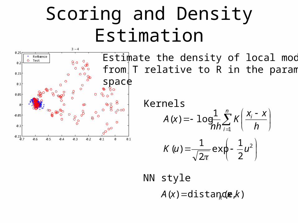
Scoring and Density Estimation

n

i

i

h

xxK

nhxA

1

1log)(

2

2

1exp

2

1)( uuK

),(distance)( kxxA R

-0.7 -0.6 -0.5 -0.4 -0.3 -0.2 -0.1 0 0.1-0.15

-0.1

-0.05

0

0.05

0.1

0.15

0.2

0.253 -- 4

ReferenceTest Estimate the density of local models

from T relative to R in the parameterspace

Kernels

NN style

Determining a Null Distribution

• Score function provides a continuous estimate but some tasks require hard cutoff

• Null Distribution: – the distribution of anomaly scores

we would expect to see if the data was completely normal

• Resample R and generate empirical distribution from block cross-validation

• Provides hypothesis testing framework for sounding alarms

0 100 200 300 400 500 600 700 800 900 10000

0.1

0.2

0.3

0.4

0.5

0.6

0 0.2 0.4 0.6 0.8 1 1.2 1.40

20

40

60

80

100

120

140

160

180

Anomaly score

Empirical distribution

Computation Time

• Local Models– Linear in N (reference and test)– Cubic in number of variables (for AR)– Linear in window size (for AR)

• Density Estimation– Implemented with KD-trees– Potentially NT log NR – Can be worse in higher dimensions

Experiments

• Why evaluation is difficult

• Data sets– CD Player– Random Walk– ECG Arrhythmia– Financial Time-Series

• Comparison Algorithms– Hotelling’s T2 statistic

Hotelling’s T2 Statistic

• Commonly used in statistical process control for monitoring multivariate processes

• Basically the same as Mahalanobis distance

• Applied with time lags for patient monitoring in multivariate data (Gather et al., 2001)

21

211

21212

nn

SnnT

CD Player

• Data from mechanical cd player arm– Two inputs relating to actuators (u1,u2)– Two outputs relating to position accuracy (y1,y2)

0 200 400 600 800 1000 1200-1.5

-1

-0.5

0

0.5

1

1.5

0 200 400 600 800 1000 1200-2

-1

0

1

2target

0 200 400 600 800 1000 12000

0.1

0.2

0.3

0.4

0.5anomaly score

Output variable y1: artificial anomaly

0 200 400 600 800 1000 1200-1

-0.5

0

0.5

1target

0 200 400 600 800 1000 12000.05

0.1

0.15

0.2

0.25anomaly score

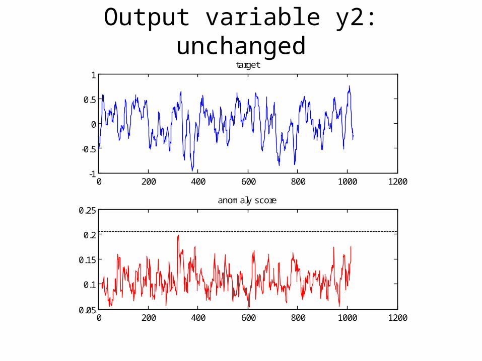
Output variable y2: unchanged

0 200 400 600 800 1000 1200-2

-1

0

1

2target

0 200 400 600 800 1000 12000

20

40

60

80

100anomaly score

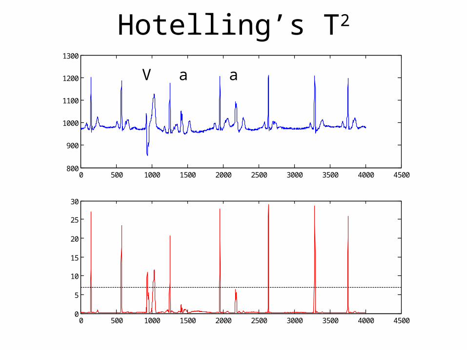
Hotelling’s T2

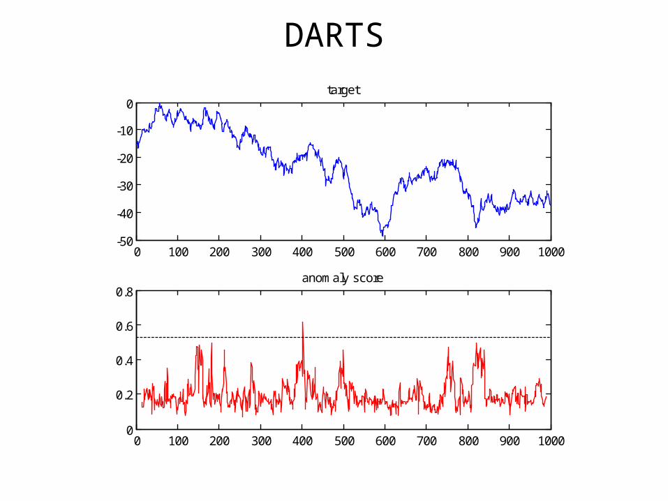
Random Walk

• No anomalies in random walk data

0 100 200 300 400 500 600 700 800 900 1000-20

-10

0

10

20

30

40

50target training data

0 100 200 300 400 500 600 700 800 900 1000-50

-40

-30

-20

-10

0target

0 100 200 300 400 500 600 700 800 900 10000

0.2

0.4

0.6

0.8anomaly score

DARTS

0 100 200 300 400 500 600 700 800 900 1000-50

-40

-30

-20

-10

0target

0 100 200 300 400 500 600 700 800 900 10000

10

20

30

40anomaly score

Hotelling’s T2

Cardiac Arrhythmia Data

• Electrocardiogram traces from MIT-BIH• Collected to study cardiac dynamics and

arrhythmias• Every beat annotated by two cardiologists• 30 minute recording @ 360 Hz• Roughly 650,000 points, 2000 beats• Points 100-3000 reference set• remainder is test data

Cardiac Reference Data

0 500 1000 1500 2000 2500 3000950

1000

1050

1100

1150

1200

1250

0 500 1000 1500 2000 2500 3000 3500 4000 4500800

900

1000

1100

1200

1300

0 500 1000 1500 2000 2500 3000 3500 4000 45000

0.1

0.2

0.3

0.4

0.5

DARTS

V a a

0 500 1000 1500 2000 2500 3000 3500 4000 4500800

900

1000

1100

1200

1300

0 500 1000 1500 2000 2500 3000 3500 4000 45000

5

10

15

20

25

30

Hotelling’s T2

V a a

0 500 1000 1500 2000 2500 3000 3500950

1000

1050

1100

1150

1200

1250

0 500 1000 1500 2000 2500 3000 35000

0.1

0.2

0.3

0.4

0.5

DARTS

j j j

0 500 1000 1500 2000 2500 3000 3500900

1000

1100

1200

1300

0 500 1000 1500 2000 2500 3000 35000

0.1

0.2

0.3

0.4

0.5

DARTS

a

TP/FP Statistics

Threshold TP TN FP FN Sensitivity Selectivity

97% 313 984 127 66 82.6% 71.1%

98% 285 1040 71 94 75.2% 80.1%

99% 205 1088 23 174 54.1% 89.9%

Sensitivity = TP / (TP + FN)Selectivity = TP / (TP + FP)

Japanese Financial Data

• Monthly data from 1983-2003• Variables:

– Monetary base– National bond interest rate– Wholesale price index– Index of industrial produce– Machinery orders– Exchange rate yen/dollar

• True anomalies unknown – subjective evaluation by expert

1990 1992 1994 1996 1998 2000 2002 2004-1

-0.5

0

0.5national bond interest rate 1991-2003

1990 1992 1994 1996 1998 2000 2002 20040

0.1

0.2

0.3

0.4

0.5national bond interest rate anomaly score

DARTS: Bond Rate

1990 1992 1994 1996 1998 2000 2002 2004-0.1

0

0.1

0.2

0.3

0.4monetary base 1991-2003

1990 1992 1994 1996 1998 2000 2002 20040

0.05

0.1

0.15

0.2monetary base anomaly score

DARTS: Monetary Base

1990 1992 1994 1996 1998 2000 2002 2004-0.03

-0.02

-0.01

0

0.01

0.02wholesale price index 1991-2003

1990 1992 1994 1996 1998 2000 2002 20040

0.02

0.04

0.06wholesale price index anomaly score

DARTS: Wholesale Price Index

1990 1992 1994 1996 1998 2000 2002 2004-0.15

-0.1

-0.05

0

0.05

0.1index industrial produce 1991-2003

1990 1992 1994 1996 1998 2000 2002 20040

0.05

0.1

0.15

0.2index industrial produce anomaly score

DARTS: Index Industrial Produce

1990 1992 1994 1996 1998 2000 2002 2004-0.4

-0.2

0

0.2

0.4machinery orders 1991-2003

1990 1992 1994 1996 1998 2000 2002 20040.05

0.1

0.15

0.2

0.25machinery orders anomaly score

DARTS: Machinery Orders

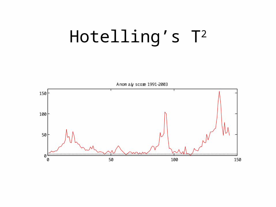
Hotelling’s T2

0 50 100 1500

50

100

150

Anomaly score 1991-2003

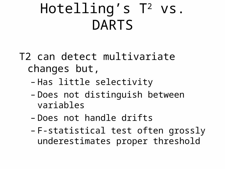
Hotelling’s T2 vs. DARTS

T2 can detect multivariate changes but,– Has little selectivity– Does not distinguish between variables– Does not handle drifts– F-statistical test often grossly underestimates

proper threshold

Limitations of DARTS

• Suitability of local models

• Window-size and sensitivity

• Number of parameters

• Overlapping data

• Efficiency of KD-tree

• Explanation

Related Work

• Limit checking

• Discrepancy checking

• Autoregressive models

• Unusual patterns

• HMM’s

Conclusions

• DARTS framework

• Data -> local models -> parameter space -> density estimate

• Provides hypothesis testing framework for flagging anomalies

• Promising results on a variety of real and synthetic problems

DARTS Framework

1. Preprocess R and T

2. Select target variable and create local models from R

3. Create local models from T

4. Compare models of T to R in space P

5. Compute Null Distribution

6. Repeat steps 2-5 for each variable