A fully nonlinear iterative solution method for

self-similar potential flows with a free boundary

A. Iafrati

INSEAN-CNR - The Italian Ship Model Basin, Rome, Italy

Abstract

An iterative solution method for fully nonlinear boundary value problemsgoverning self-similar flows with a free boundary is presented. Specifically,the method is developed for application to water entry problems, which canbe studied under the assumptions of an ideal and incompressible fluid withnegligible gravity and surface tension effects. The approach is based on apseudo time stepping procedure, which uses a boundary integral equationmethod for the solution of the Laplace problem governing the velocity po-tential at each iteration. In order to demonstrate the flexibility and thecapabilities of the approach, several applications are presented: the classicalwedge entry problem, which is also used for a validation of the approach,the block sliding along an inclined sea bed, the vertical water entry of a flatplate and the ditching of an inclined plate. The solution procedure is alsoapplied to cases in which the body surface is either porous or perforated.Comparisons with numerical or experimental data available in literature arepresented for the purpose of validation.

Keywords: free surface flows, water entry problems, potential flows,boundary integral methods, free boundary problems, self-similar flows

1. Introduction

The water entry flow is highly nonlinear and is generally characterisedby thin jets, as well as sharp velocity and pressure gradients. As a freeboundary problem, the solution is further complicated from the mathematicalviewpoint by the fact that a portion of the domain boundary, which is thefree surface, is unknown and has to be derived as a part of the solution.At least in the early stage of the water entry, viscous effects are negligible

Preprint submitted to Computer Methods in Applied Mechanics and EngineeringAugust 6, 2021

arX

iv:1

212.

6699

v2 [

phys

ics.

flu-

dyn]

19

Jan

2013

and thus the fluid can be considered as ideal. Moreover, provided the anglebetween the free surface and the tangent to the body at the contact point isgreater than zero, compressible effects are negligible Korobkin & Pukhnachov(1988) and the fluid can be considered as incompressible.

Several approaches dealing with water entry problems have been devel-oped within the potential flow approximation over the last twenty years,which provide the solution in the time domain, e.g. Zhao & Faltinsen (1993);Battistin & Iafrati (2003); Mei et al. (1999); Wu et al. (2004); Xu et al.(2008, 2010) just to mention a few of them. Time domain approaches are

characterised by a high level of flexibility, as they can be generally appliedto almost arbitrary body shapes and allow to account for the variation ofthe penetration velocity in time. However, depending on the shape of thebody and on the entry velocity, the solution can be profitably written in aself-similar form by using a set of time dependent spatial variables. In thisway, the initial boundary value problem is transformed into a boundary valueproblem, e.g. Semenov & Iafrati (2006); Faltinsen & Semenov (2008). Itis worth noticing that sometime the solution formulated in terms of timedependent variables is not exactly time independent, but it can be approxi-mated as such under some additional assumptions. Problems of this kind arefor instance those discussed in King & Needham (1994); Iafrati & Korobkin(2004); Needham et al. (2008) where the solutions can be considered as

self-similar in the limit as t→ 0+.Although avoiding the time variable reduces the complexity significantly,

the problem remains still nonlinear as a portion of the boundary is still un-known and the conditions to be applied over there depends on the solution.Several approaches have been proposed for the solution of the fully nonlin-ear problem since the very first formulation by Dobrovol’skaya (1969), whoexpressed the solution of the problem in terms of a nonlinear, singular, in-tegrodifferential equation. The derivation of the solution function is rathertricky, though (Zhao & Faltinsen , 1993). An approach which has some sim-ilarities with that proposed by Dobrovol’skaya (1969), has been proposedin Semenov & Iafrati (2006) where the solution is derived in terms of twogoverning functions, which are the complex velocity and the derivative of thecomplex potential defined in a parameter domain. The two functions areobtained as the solution of a system of an integral and an integro-differentialequation in terms of the velocity modulus and of the velocity angle to the freesurface, both depending on the parameter variable. This approach provedto be rather accurate and flexible (Faltinsen & Semenov , 2008; Semenov &

2

Yoon , 2009), although it is not clear at the moment if that approach can beeasily extended to deal with permeable conditions at the solid boundaries.

Another approach is proposed in Needham et al. (2008), which generalisethe method also used in King & Needham (1994) and Needham et al. (2007),uses a Newton iteration method for the solution of the nonlinear boundaryvalue problem. The boundary conditions are not enforced in a fully nonlinear,though. Both the conditions to be applied and the surface onto which theconditions are applied are determined in an asymptotic manner, which istruncated at a certain point.

In this work an iterative, fully nonlinear, solution method for a class ofboundary value problems with free boundary is presented. The approach isbased on a pseudo-time-stepping procedure, basically similar to that adoptedin time domain simulations of the water entry of arbitrary shaped bodies(Battistin & Iafrati , 2003; Iafrati & Battistin , 2003; Iafrati , 2007). Differ-ently from that, the solution method exploits a modified velocity potentialwhich allows to significantly simplify the boundary conditions at the free sur-face. By using a boundary integral representation of the velocity potential, aboundary integral equation is obtained by enforcing the boundary conditions.A Dirichlet condition is applied on the free surface, whereas a Neumann con-dition is enforced at the body surface. In discrete form, the boundary isdiscretized by straight line panels and piecewise constant distributions of thevelocity potential and of its normal derivative are assumed.

As already said, water entry flows are generally characterised by thinjets developing along the body surface or sprays detaching from the edges offinite size bodies. An accurate description of the solution inside such thinlayers requires highly refined discretizations, with panel size of the order ofthe jet thickness. A significant reduction of the computational effort canbe achieved by cutting the thin jet off the computational domain withoutaffecting the accuracy of the solution substantially. However, there are somecircumstances in which it is important to extract some additional informationabout the solution inside the jet, e.g. the jet length or the velocity of the jettip. For those cases, a shallow water model has been developed which allowsto compute the solution inside the thinnest part of the jet in an accurateand efficient way by exploiting the hyperbolic structure of the equations. Aspace marching procedure is adopted, which is started at the root of the jetby matching the solution provided by the boundary integral representation.

The solution method is here presented and applied to several water entryproblems. It is worth noticing that the method has been adopted in the

3

past to study several problems, but was never presented in a unified manner.For this reason, in addition to some brand new results, some results of ap-plications of the method which already appeared in conference proceedingsor published paper are here briefly reviewed. The review part is not aimedat discussing the physical aspects but mainly at showing, with a unified no-tation, how the governing equations change when the model is applied todifferent contexts. Solutions are presented both for self-similar problems andfor problems which are self-similar in the small time limit. Applications arealso presented for bodies with porous or perforated surfaces where the theboundary condition at the solid boundary depends on the local pressure.

The mathematical formulation and the boundary value problem are de-rived in section 2 for the self-similar wedge entry problem with constant veloc-ity. The disrete method is illustrated in section 3, together with a discussionover the shallow water model adopted for the thin jet layer. The applicationsof the proposed approach to the different problems are presented in section4 along with a discussion about the changes in the governing equations.

2. Mathematical formulation

The mathematical formulation of the problem is here derived referringto the water entry of a two-dimensional wedge, under the assumption ofan ideal and incompressible fluid with gravity and surface tension effectsalso neglected. The wedge, which has a deadrise angle γ, touches the freesurface at t = 0 and penetrates the water at a constant speed V . Under theabove assumptions, the flow can be expressed in terms of a velocity potential

4

φ(x, y, t) which satisfies the initial-boundary value problem

∇2φ = 0 Ω(t) (1)

∂φ

∂n= 0 x = 0 (2)

∂φ

∂n= V cos γ y = −V t+ x tan γ (3)

∂φ

∂t+

1

2u2 = 0 H(x, y, t) = 0 (4)

DH

Dt= 0 H(x, y, t) = 0 (5)

H(x, y, 0) = 0 y = 0 (6)

φ(x, y, 0) = 0 y = 0 (7)

φ(x, y, t) → 0 (x2 + y2)→∞ (8)

where Ω(t) is the fluid domain, H(x, y, t) = 0 is the equation of the free sur-face, n is the normal to the fluid domain oriented inwards and x, y representthe horizontal and vertical coordinates, respectively. Equation (2) representsthe symmetry condition about the y axis. In equation (4) u = ∇φ is thefluid velocity. It is worth remarking that the free surface shape, i.e. thefunction H(x, y, t), is unknown and has to be determined as a part of thesolution. This is achieved by satisfying equations (4) and (5) which rep-resent the dynamic and kinematic boundary conditions at the free surface,respectively.

By introducing the new set of variables:

ξ =x

V tη =

y

V tϕ =

φ

V 2t, (9)

the initial-boundary value problem can be recast into a self-similar problem,which is expressed by the following set of equations:

∇2ϕ = 0 Ω (10)

ϕξ = 0 ξ = 0 (11)

ϕν = cos γ η = −1 + ξ tan γ (12)

ϕ− (ξϕξ + ηϕη) +1

2

(ϕ2ξ + ϕ2

η

)= 0 h(ξ, η) = 0 (13)

−(ξhξ + ηhη) + (hξϕξ + hηϕη) = 0 h(ξ, η) = 0 (14)

ϕ → 0 ξ2 + η2 →∞ (15)

5

where Ω is fluid domain, h(ξ, η) = 0 is the equation of the free surface andν is the unit normal to the boundary, which is oriented inward the fluiddomain.

Despite the much simpler form, the boundary value problem governingthe self-similar solution is still rather challenging as the free surface shape isunknown and nonlinear boundary conditions have to be enforced on it. Thefree surface boundary conditions can be significantly simplified by introduc-ing a modified potential S(ξ, η) which is defined as

S(ξ, η) = ϕ(ξ, η)− 1

2ρ2 (16)

where ρ =√ξ2 + η2. By substituting equation (16) into the kinematic con-

dition (14), it follows that ∇S · ∇h = 0, which is

Sν = 0 (17)

on the free surface h = 0. Similarly, by substituting equation (16) into thedynamic condition (13), it is obtained that

S +1

2

(S2ξ + S2

η

)= 0

on the free surface. By using equation (17), the above equation becomes

S +1

2S2τ = 0 ⇒ Sτ = ±

√−2S , (18)

where τ is the arclength measured along the free surface (Fig. 1).By combining all equations together, we arrive at the new boundary value

problem

∇2ϕ = 0 Ω (19)

ϕξ = 0 ξ = 0 (20)

ϕν = cos γ η = −1 + ξ tan γ (21)

ϕ = S +1

2ρ2 h(ξ, η) = 0 (22)

Sτ = ±√−2S h(ξ, η) = 0 (23)

Sν = 0 h(ξ, η) = 0 (24)

S → −1

2ρ2 ρ→∞ (25)

solution of which is derived numerically via a pseudo-time stepping procedurediscussed in detail in the next section.

6

3. Iterative Solution Method

The solution of the boundary value problem (19)-(24) is obtained by apseudo-time stepping procedure similar to that adopted for the solution ofthe water entry problem in time domain (Battistin & Iafrati , 2003, 2004).The procedure is based on an Eulerian step, in which the boundary valueproblem for the velocity potential is solved, and a Lagrangian step, in whichthe free surface position is moved in a pseudo-time stepping fashion and thevelocity potential on it is updated.

3.1. Eulerian substep

Starting from a given free surface shape with a corresponding distributionof the velocity potential on it, the velocity potential at any point xP =(ξP , ηP ) ∈ Ω is written in the form of boundary integral representation

ϕ(xP ) =

∫SS∪SB∪S∞

(∂ϕ(xQ)

∂νQG(xP − xQ)− ϕ(xQ)

∂G(xP − xQ)

∂νQ

)dSQ ,

(26)where xQ = (ξQ, ηQ) ∈ ∂Ω. In the integrals, SB and SS denote thebody contour and free surface, respectively, S∞ the boundary at infinity andG(x) = log (|x|) /2π the free space Green’s function of the Laplace operatorin two-dimensions.

The velocity potential along the free surface is assigned by equations (22)and (23), whereas its normal derivative on the body contour is given byequation (21). In order to derive the velocity potential on the body and thenormal derivative at the free surface the limit of equation (26) is taken asxP → ∂Ω. Under suitable assumptions of regularity of the fluid boundary,for each xP ∈ ∂Ω it is obtained

1

2ϕ(xP ) =

∫SS∪SB∪S∞

(∂ϕ(xQ)

∂νQG(xP − xQ)− ϕ(xQ)

∂G(xP − xQ)

∂νQ

)dSQ .

(27)The above integral equation with mixed Neumann and Dirichlet boundaryconditions, is solved numerically by discretizing the domain boundary intostraight line segments along which a piecewise constant distribution of thevelocity potential and of its normal derivative are assumed. Hence, in discreteform, it is obtained

aiϕi +

NB∑j=1

ϕjdij −NB+NS∑j=NB+1

ϕν,jgij = eiϕi −NB+NS∑j=NB

ϕjdij +

NB∑j=1

ϕν,jgij , (28)

7

where NB and NS indicate the number of elements on the body and on thefree surface, respectively, with (ai, ei) = (1/2, 0) if i ∈ (1, NB) and (ai, ei) =(0,−1/2) if i ∈ (NB, NB + NS). In (28) gij and dij denote the influencecoefficients of the segment j on the midpoint of the segment i related to Gand Gν , respectively. It is worth noticing that the when xP lies onto oneof the segments representing the free surface, the integral of the influencecoefficient dij is evaluated as the Cauchy principal part. The symmetrycondition about the ξ = 0 axis is enforced by accounting for the image whencomputing the influence coefficients.

The size of the panels adopted for the discretization is refined duringthe iterative process in order to achieve a satisfactory accuracy in the higlycurved region about the jet root. Far from the jet root region, the panel sizegrows with a factor which is usually 1.05.

The linear system (28) is valid provided the computational domain isso wide that condition (15) is satisfied at the desired accuracy at the farfield. A significant reduction of the size of the domain can be achieved byapproximating the far field behaviour with a dipole solution. When suchan expedient is adopted, a far field boundary SF is introduced at a shortdistance from the origin, along which the velocity potential is assigned asCDϕD where ϕD is the dipole solution

ϕD =η

ξ2 + η2.

Along the boundary SF , the normal derivative is derived from the solutionof the boundary integral equation. Let NF denote the number of elementslocated on the far field boundary, the discrete system of equations becomes

aiϕi +

NB∑j=1

ϕjdij −NB+NS+NF∑j=NB+1

ϕν,jgij + CD

NF∑j=NB+NS+1

ϕD,jdij = eiϕi−

NB+NS+NF∑j=NB+1

ϕjdij +

NB∑j=1

ϕν,jgij , (29)

where i ∈ (1, NB +NS +NF ). An additional equation is needed to derive theconstant of the dipole CD together with the solution of the boundary valueproblem. There is no unique solution to assign such additional condition.Here this additional equation is obtained by enforcing the condition that the

8

total flux across the far field boundary has to equal that associated to thedipole solution, which in discrete form reads (Battistin & Iafrati , 2004)

−NB+NS+NF∑j=NB+NS+1

ϕν,j∆sj + CD

NB+NS+NF∑j=NB+NS+1

ϕDν,j∆sj = 0 . (30)

The solution of the linear system composed by equations (29) and (30),provides the velocity potential on the body contour and its normal derivativeon the free surface. Hence, the tangential and normal derivatives of themodified velocity potential can be computed as

Sτ = ϕτ − ρρτ , Sν = ϕν − ρρν (31)

allowing to check if the kinematic condition on the free surface (24) is satis-fied. Unless the condition is satisfied at the desired accuracy, the free surfaceshape and the distribution of the velocity potential on it are updated and anew iteration is made.

3.2. Update of free surface shape and velocity potential

The solution of the boundary value problem makes available the normaland tangential derivatives of S at the free surface. A new guess for thefree surface shape is obtained by displacing the free surface with the pseudovelocity field ∇S, which is

Dx

Dt= ∇S . (32)

Equation (32) is integrated in time (actually, it would be more correct to saypseudo time) by a second order Runge Kutta scheme. The time interval ischosen so that the displacement of the centroid in the step is always smallerthan one fourth of the corresponding panel size. Once the new shape isavailable, the modified velocity potential on it is initialized and the velocitypotential is derived from equation (22). At the intersection of the free surfacewith the far field boundary the velocity potential is provided by the dipolesolution, by using the constant of the dipole obtained from the solution ofthe boundary value problem at the previous iteration. The value of thevelocity potential is used to compute the corresponding modified velocitypotential from equation (22) and then the dynamic boundary condition (23)is integrated along the free surface moving back towards the intersection withthe body contour, thus providing the values of S and ϕ on the new guess.

9

For the wedge entry problem, at the far field, the modified velocity po-tential behaves as S → −ρ2/2 and thus, Sτ ' −ρ as ρ→∞ (Fig. 1). In thiscase the boundary condition can be easily integrated along the free surface,in the form

S = −1

2(τ + C)2 . (33)

By assuming that the free surface forms a finite angle with the body contour,the boundary conditions (21) and (24) can be both satisfied at the intersec-tion point only if Sτ = 0 and thus S = 0. From equation (33) it followsthat the conditions are satisfied if C = 0 and τ is taken with origin at theintersection point, i.e.

S = −1

2τ 2 . (34)

Although equation (34) holds for the final solution, the conditions are notsatisfied for an intermediate solution. In this case, for the new free surfaceshape the curvilinear abscissa τ is initialized starting from the intersectionwith the body contour and the constant C is chosen to match the value of themodified velocity potential at the intersection with the far field boundary.Once the distribution of the modified velocity potential on the free surfaceis updated, the velocity potential is derived from equation (22), and theboundary value problem can be solved.

Additional considerations are deserved by the choice of ∇S as pseudovelocity field. It is easy to see that with such a choice, once the final solu-tion has been reached and Sν approaches zero all along the free surface, thedisplacements of the centroids are everywhere tangential to the free surface,thus leaving the free surface shape unchanged. However, this is not enoughto explain why the use of Sν as normal velocity drives the free surface towardsthe solution of the problem. By differentiating twice in τ equation (33) wehave that Sττ = −1. From equation (16), it is Sνν + Sττ = −2 and then onthe free surface

Sνν = −2− Sττ = −1 .

According to the kinematic condition (24) Sν = 0 on the free surface, so thatif Sνν < 0 we have Sν < 0 in the water domain, which implies that using Sνas normal velocity drives the free surface towards the solution (Fig. 2).

3.3. Jet modelling

Water entry flows often generates thin sprays along the body contours.An accurate description of such thin layer by a boundary integral representa-

10

tion requires highly refined discretizations, with panel dimensions comparableto the local thickness. Beside increasing the size of the linear system to besolved, the small panel lenghts in combination to the high velocity character-izing the jet region yields a significant reduction of the time step making adetailed description of the solution highly expensive from the computationalstandpoint.

Despite the effort required for its accurate description, the jet does notcontribute significantly to the hydrodynamic loads acting on the body, whichis doubtless the most interesting quantity to be evaluated in a water entryproblem. Indeed, due to the small thickness, the pressure inside the spray isessentially constant and equal to the value it takes at the free surface, whichis p = 0. This is the reason why rather acceptable estimates of the pressuredistribution and total hydrodynamic loads can be obtained by cutting off thethinnest part of the jet, provided a suitable boundary condition is appliedat the truncation. In the context of time domain solutions, the cut of thejet was exploited for instance in Battistin & Iafrati (2003) in which the jetis cut at the point where the angle between the free surface and the bodycontour drops below a threshold value.

A similar cut can be adopted in the context self-similar problems discussedhere. The truncated part is accounted for by assuming that the normalvelocity at the truncation of the jet equals the projection on the normaldirection of the velocity at the free surface. From the sketch provided inFig. 3, τ ∗, which denotes the value of the arclength at the intersection betweenthe free surface and the jet truncation, is different from zero and thus, fromequation (34) it follows

Sτ (τ∗) = −τ ∗ . (35)

The value τ ∗ is derived by initializing the arclength on the free surface asτ = τ + τ ∗ and matching the velocity potential at the far field with theasymptotic behaviour. If the computational domain is large enough, thematching is established in terms of the tangential velocity and thus, fromequation (25), we simply get that

τ ∗ = ρ− τ .

When the dipole solution CDϕD is used to approximate the far field solution,τ ∗ is determined by matching the velocity potential and then, by equations(22) and (34), we get

τ ∗ = (ρ2 − 2CDϕD)1/2 − τ .

11

The tangential velocity at the intersection of the free surface with the jettruncation line can be computed from

ϕτ = Sτ + ρρτ , (36)

where Sτ comes from equation (35). Hence, the normal velocity to be usedas boundary condition at the jet truncation is derived as

ϕν = ϕτ cos β , (37)

where β is angle formed by body contour with the tangent at the free surfacetaken at the intersection with jet truncation line.

Although very efficient and reasonably accurate, such simplified modelsdo not allow to derive any information in terms of wetted surface and jetspeed. An alternative approach, which provides all the information in arather efficient way, exploits the shallowness of the jet layer. In order toexplain the model, it is useful to consider the governing equations in a localframe of reference with λ denoting the coordinate along the body and µ =f(λ) the local thickness (Fig. 3). The kinematic boundary condition (24)becomes

Sµ = Sλfλ on µ = f(λ) . (38)

From the definition (16), it follows that ∇2S = −2. Integration of theabove equation across the jet thickness, i.e. along a λ = const line, provides∫ f(λ)

0

Sλλ(λ, µ)dµ+ [Sµ(λ, µ)]µ=f(λ)µ=0 = −2f(λ) . (39)

By exploting the body boundary conditions on the body surface, we finallyget (Korobkin & Iafrati , 2006)

d

dλ

∫ f(λ)

0

Sλ(λ, µ)dµ = −2f(λ) , (40)

which can be further simplified by neglecting the variations of the modifiedvelocity potential across the jet layer, thus arriving to[

Sλ(λ)f(λ)]λ

+ 2f(λ) = 0 , (41)

where S(λ) = S (λ, f(λ)) ' S(λ, µ). In terms of S(λ) the kinematic condition(38) reads

Sλ = − Sτ√1 + f 2

λ

(42)

12

Equations (41) and (42), together with the dynamic boundary condition(34) can be used to build an iterative, space marching procedure which, atthe jet root, matches the solution provided by the boundary integral formu-lation in the bulk of the fluid. The most relevant point of the procedure arediscussed here, whereas a more detailed description can be found in Korobkin& Iafrati (2006).

By using a finite difference discretization of equation (41), the followingequation for the jet thickness is obtained

fk(i+ 1) = ωfk−1(i+ 1)− (1− ω)f(i)

[∆λ− Sλ(i)

∆λ+ Sk−1λ (i+ 1)

]. (43)

As Sλ(i + 1) and f(i + 1) are both unknown, the solution is derived bysubiterations. In equation (43) k is the subiteration number and ω is arelaxation parameter, which is usually taken as 0.9. Once the new estimateof the local thickness fk(i+1) is available, it is used in the kinematic condition(42) to evaluate Skλ(i+ 1) as

Skλ(i+ 1) = − Skτ (i+ 1)√1 +

[fkλ (i+ 1)

]2 , (44)

where the derivative of the thickness is evaluated in discrete form as

fkλ (i+ 1) =fk(i+ 1)− f(i)

∆λ. (45)

In equation (44) the term Skτ (i+ 1) is estimated by exploiting equation (34)which provides Sτ (i) = −τ(i), and thus

Skτ (i+ 1) = Sτ (i) +√

∆λ2 + (fk(i+ 1)− f(i))2 . (46)

The system of equations (43)-(46) is solved by subiterations, which use f(i)and Sλ(i) as first guess values. All quantities at i = 1 are derived fromthe boundary integral representation, thus ensuring the continuity of thesolution. The spatial step ∆λ is assumed equal to half of the size of the firstfree surface panel attached to the jet region. Such a choice turns to be usefulfor the computation of the pressure, as discussed in the next section. Thespace marching procedure is advanced until reaching the condition |Sλ(i +1)| < ∆λ, which implies that the distance to the intersection with the bodycontour is smaller than ∆λ.

13

3.4. Pressure distribution

The pressure field on the body can be derived from the distribution of thevelocity potential. Let % denote the fluid density, the equation of the localpressure

p = −%∂φ

∂t− 1

2|u|2

,

is written in terms of the self-similar variables (9) thus leading to

ψ(ξ, η) = −ϕ+ (ϕξξ + ϕηη)− 1

2(ϕ2

ξ + ϕ2η) , (47)

where ψ = p/(%V 2) is the nondimensional pressure.When the shallow water model is activated, due to the assumptions, the

pressure in the modelled part of the jet is constant and equal to the value ittakes at the free surface, i.e zero. As a consequence, a sharp drop of the pres-sure would occur across the separation line between the bulk of the fluid andthe modelled part of the jet. In order to avoid such artificial discontinuity,the velocity potential along the body is recomputed by using the boundaryintegral representation of the velocity potential for the whole region contain-ing both the bulk of the fluid and the part of the jet modelled by the shallowwater model. As discussed in the previous section, the spatial step in thespace marching procedure of the shallow water model has been chosen ashalf of the size of the free surface panel adjacent to the modelled part of thejet. This allows a straightforward derivation of the discretization to be usedin the boundary integral representation. Two adjacent panels in the shallowwater region are used to define a single panel in the discrete boundary inte-gral representation (29). This panel has the velocity potential associated atthe mid node connecting the two shallow water elements which constitutesthe panel. On the basis of the above considerations, if NSW is the number ofsteps in the space marching procedure, the inclusion of the modelled part ofthe jet in the boundary integral representation corresponds to NSW/2 panelson the body contour and NSW/2 panel on the free surface, with a total ofNSW additional equations in (29). As usual, a Neumann boundary conditionis applied to the panels lying along the body contour, and a Dirichlet con-dition is applied to the panels lying on the free surface. It is shown in thefollowing that including the shallow water solution in the boundary integralrepresentation results in a much smoother pressure distribution about theroot of the jet, whereas the remaining part is essentially unchanged.

14

3.5. Porous and perforated contours

The solution procedure is also applicable to problems in which the solidboundary is permeable, provided the boundary condition can be formulatedas a function of the pressure. In these case, of course, an accurate predictionof the pressure distribution is mandatory.

Possible examples are represented by porous or perforated surfaces. Ina porous surface the penetration velocity depends on a balance between theviscous losses through the surface and the pressure jump, so that, if the V ·nis the normal velocity of the contour, the actual boundary condition is

∂φ

∂n= V · n− α0p , (48)

where α0 is a coefficient that depends on the characteristics of the porouslayer (Iafrati & Korobkin , 2005b). In a perforated surface, the flow throughthe surface is governed by a balance between the inertial terms and thepressure jump. In this case the condition is usually presented in the formMolin & Korobkin (2001)

∂φ

∂n= V · n− χ

√p/% , χ2 =

2σκ2

1− κ(49)

where σ is a dicharge coefficient which is about 0.5 and κ is the perforationratio, i.e. the ratio between the area of the holes and the total area.

In terms of the self-similar variables, both cases are still described by thesystem of equations (9)-(15) but for the body boundary condition (12) whichis rewritten as

ϕν = cos γ − f(ψ) η = −1 + ξt tan γ , (50)

where f(ψ) = α0ψ and f(ψ) = χ√ψ for porous and perforated surfaces,

respectively.Examples of water entry flows of porous or perforated bodies are presented

in the next section. The important changes operated on the solution bydifferent levels of permeability are clearly highlighted.

4. Applications

4.1. Wedge entry problem

As a first application, the computational method is applied to the waterentry with constant vertical velocity of an infinite wedge. An example of the

15

convergence process for a wedge with 10 degrees deadrise angle is shown inFig. 4.

It is worth noticing that for convenience, in the wedge entry problem, thefirst guess for the free surface is derived from the dipole solution at the farfield. Indeed, if CDϕD approximates the far field behaviour, then the freesurface elevation should behave as

η(0) =CD3ξ2

, (51)

where the constant CD is derived together with the solution of the boundaryvalue problem, as discussed in section 3. Note that, a few preliminary iter-ations are performed in order to get a better estimate of the constant CD.During these preliminary iterations the free surface varies only due to thevariation of the coefficient CD in equation (51).

Once the pseudo time stepping procedure starts, it gradually develops athin jet along the body surface. When the angle formed by the free surfacewith the body surface drops below a threshold value, usually 10 degrees,the jet is truncated or the shallow water model is activated. This process isshown in the left picture of Fig. 4 where, for the sake of clarity, the shallowwater region is not displayed.

The convergence in terms of pressure distribution is shown in Fig. 5 alongwith a close up view of the jet root region. It can be noticed that the useof the shallow water solution within the boundary integral representationmakes the pressure very smooth about the transition.

Due to the use of the ∇S as a pseudo velocity field for the displacementof the free surface panels, the achievement of convergence implies that thereis no further motion of the free surface in the normal direction, and thusthe kinematic condition (17) is satisfied. A more quantitative understandingof the convergence in terms of the kinematic condition is provided by thequantity

K =

∫SS

S2ν ds . (52)

The behaviour of K versus the iteration number is displayed in Fig. 6, whichindicates that K diminishes until reaching a limit value that diminishes whenrefining the discretization.

In Fig. 7 the free surface profiles obtained for different deadrise anglesare compared. In the figure, two solutions, largely overlapped, are drawn

16

γ Cp = 2ψ ηmaxPresent ZF Present ZF

7.5 140.1 140.59 0.5601 0.562310 77.6 77.85 0.5538 0.555620 17.7 17.77 0.5079 0.508730 6.86 6.927 0.4217 0.424340 3.23 3.266 0.2946 0.2866

Table 1: Comparison between the results provided by the present solver and the corre-sponding data derived by the self-similar solution in Zhao & Faltinsen (1993).

for the 10 degree wedge which refers to two different discretizations, withminimum panel size of 0.04 and 0.01 for the coarse and fine grids, respectively.Similarly, two solutions are drawn for the 60 degrees case, one which makesuse of the shallow water model and a second solution in which the jet isdescribed by the boundary integral representation. At such deadrise angles,the angle at the tip, which is about 15 degrees, is large enough to allow anaccurate and still efficient description of the solution within the standardboundary integral representation.

It is worth noticing that, as the solution is given in terms of the self-similarvariables (9), the length of the jet in terms of those variables

lj =√ξ2j + η2j , (53)

is also an index of the propagation velocity of the tip. For the present prob-lem, according to equations (9) the scaling from the self-similar to the phys-ical variables is simply linear and thus the lj is just the tip speed. The jetlength versus the deadrise angle, which is drawn in Fig. 8, approaches a 1/γtrend for γ ≤ 30 degrees.

A comparison of the pressure distribution obtained for different deadriseangles is provided in Fig. 9. The results show that, up to 40 degrees deadriseangle, the pressure distribution is characterised by a pressure peak occurringabout the root of the jet whereas, at larger deadrise angles, the maximumpressure occur at the wedge apex. As for the free surface shape, also forthe pressure distribution two solutions are drawn for the cases at 10 and 60deadrise angles, which are essentially overlapped.

For validation of the results, some relevant quantities are extracted andcompared with corresponding data computed by the Dobrovol’skaya (1969)

17

α0, χ Porous PerforatedCpmax ηmax lj Cpmax ηmax lj

0.0 6.86 0.4217 5.6612 6.86 0.4217 5.66120.02 6.59 0.4052 5.5527 6.69 0.4098 5.59300.05 6.20 0.3807 5.4086 6.43 0.3988 5.49100.10 5.68 0.3451 5.2084 6.02 0.3697 5.33500.20 4.88 0.2887 4.9145 5.33 0.3127 5.06100.30 4.28 0.2442 4.7100 4.74 0.2686 4.83390.40 3.83 0.2150 4.5610 4.24 0.2285 4.64620.50 3.45 0.1856 4.4460 3.81 0.1956 4.4912

Table 2: Effect of the porosity coefficient and of the perforation ratio on some relevantparameters for a 30 degrees wedge.

model in Zhao & Faltinsen (1993). The comparison is established in termsof the maximum pressure coefficient, which is 2ψmax, and of the verticalcoordinate of the point along the body where the pressure gets the peak,ηmax = ξmax tan γ − 1. The comparison, shown in Table 1, displays a rathergood agreement for all the deadrise angles.

When the body surface is either porous or perforated, a flow throughthe solid boundary occurs which grows with the local pressure. As shownin Fig. 9, for deadrise angles smaller than 40 degrees the pressure takes themaximum at the root of the jet, and this causes a shrinking, and a subsequentshortening, of the jet. The changes in the free surface shape caused by theporosity of the surface on a 10 degrees wedge are shown in Fig. 10 where theshrinking of the jet is clearly highlighted. From the corresponding pressuredistributions, which are given in the left picture, it can be seen that evenlow porosity levels provide an important reduction in the pressure peak, andthe peak itself is shifted down towards the wedge apex, thus leading to ashortening of the region of the body exposed to the pressure. Beside thereduction of the peak value, the pressure displays a significant reduction alsoin the remaining part of the body, and all those effects combined togetherimplies an significant reduction of the total load acting on the body.

Similar results are shown also for a 30 degrees wedge, in Fig. 11, wheresolutions for perforated surfaces are compared. Quantitatively, the differ-ences in terms of Cp, ηmax and lj when varying the porous or the perforationcoefficient are provided in Table 2.

18

4.2. Sliding block

As a second application, the method is adopted to study the flow gen-erated when a solid block slides along a sloping bed (Fig. 12). This flowconfiguration resembles that generated at coastal sites when massive landslides along the sea bed giving rise to tsunamis. The study can help in un-derstanding which are the conditions in terms of the angle of the front andbed slope which result in the larger velocities. The possibility of accountingfor the permeability of the mass is exploited as well.

This problem and all the physical implications were already addressedand discussed in Iafrati et al. (2007). As explained in the introduction, theapplication is here shortly reviewed, focusing the attention on the changes tobe operated to the boundary value problem formulated above. Some otheraspects of the solutions are highlighted as well.

By assuming a constant entry velocity, which is acceptable in an earlystage, the flow is self-similar and can be described by the same approachpresented above. The only difference concerns the boundary conditions onthe bed and on the front which are

ϕν = 0 on η = −ξ tan θ (54)

and

ϕν = sin(γ + θ)− f(ψ) on η = ξ tan γ − sin(γ + θ)

cos γ(55)

where, as aforesaid, f(ψ) accounts for the permeability of the block and θ isthe inclination of the sea bed (Fig. 12). In this case the solid boundary isrepresented by both the bed and the block front, but only the latter can bepermeable.

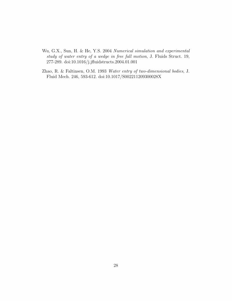
The free surface profiles generated by a block sliding over sea beds withdifferent slopes and different inclinations of the block are shown in Fig. 13.When the shallow water model is exploited, the free surface portions belong-ing to the bulk of the fluid and to the shallow water region are displayed,along with the boundary between the two domains. For the case with γ = 60degrees, the results indicate that the jet length grows, i.e. the tip movesfaster, when the beach slope increases from 10 to 40 and decays for largerslopes. Results are similar for the case γ = 90 degrees, although the max-imum is achieved for a bed slope of 30 degrees. For an inclination of thefront of 120 degrees the results show that the jet length decays monotoni-cally as the beach slope increases. Quantitatively, the results are summarizedin Table 3.

19

θ γ = 60 γ = 90 γ = 120ξT ηT lJ ξT ηT lJ ξT ηT lJ

10 1.822 1.277 1.474 0.9848 1.196 1.196 0.3894 0.8576 1.23220 2.003 1.500 1.732 0.9397 1.261 1.261 0.2940 0.7764 1.16330 2.097 1.631 1.884 0.8660 1.249 1.249 0.2039 0.6468 0.867040 2.112 1.689 1.951 0.7660 1.176 1.176 0.1182 0.4794 0.621150 2.056 1.682 1.942 0.6428 1.050 1.050 4.8543E-02 0.2632 0.330960 1.931 1.613 1.863 0.5000 0.8749 0.8749

Table 3: Coordinates of the jet tip (ξT , ηT ) and length of the jet lJ for a block withγ = 60, 90 and 120 degrees sliding along a seabed with different slopes.

In the case of a permeable front, the flow across the solid boundary makesthe jet thinner and shorter, i.e. the tip speed is lower. This can be seen fromFig. 14 where the free surface profiles obtained for a perforated block withγ = 90 degrees and θ = 40 are shown for χ = 0, 0.1 and 0.2.

4.3. Floating plate impact

The computational procedure can be also applied in contexts in whichthe problem is not strictly self-similar but is can be approximated as self-similar under additional assumptions. This is for example the case of thesudden start of a wedge originally floating on the free surface with the apexsubmerged (Iafrati & Korobkin , 2005a) or the sudden start of a floatingwedge in a weakly compressible liquid (Korobkin & Iafrati , 2006). Bothproblems are approximately self-similar in the small time limit. It can beshown that the problems can be represented by the same boundary valueproblem, aside from some differences in the coefficients appearing in thedynamic boundary condition (13) or (23).

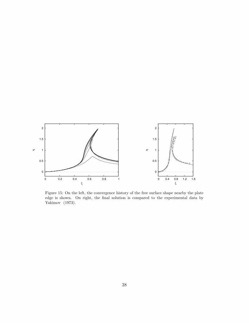
As a particular example, the water entry of a floating plate is presentedhere below. Formally, the plate entry problem is not self-similar as thebreadth of the plate introduces a length scale. By formulating the solu-tion of the problem in the form of a small time expasion, it can be shownthat the first order solution is singular at the edge of the plate. In order toresolve the singularity, an inner solution has to be formulated under set ofstretched coordinates. Hence, the inner solution has to be matched to theouter one at the far field.

20

It is worth remarking that a detailed derivation of the outer and innerproblems, as well as the matching condition, can be found in Iafrati & Ko-robkin (2004) whereas practical applications are discussed in Iafrati & Ko-robkin (2008) and Iafrati & Korobkin (2011). The problem is here discussedin order to highligth the different form of the dynamic boundary conditioncompared to the previous cases. This requires a different procedure as thedynamic boundary condition cannot be integrated analytically and, more-over, an additional unknown appears which has to be derived as a part ofthe solution. As shown in the following, the additional unknown governs theshape of the free surface.

Within a small time assumption, the problem in a close neighbourood ofthe edge is formulated in terms of the following variables:

ξ =x− 1

Bt2/3η =

y

Bt2/3ϕ =

φ√2Bt1/3

, B = (9/2)1/3 . (56)

In terms of the new variables, the problem is such that the plate is fixed andthe flow is arriving from the far field. As t → 0, in terms of the stretchedcoordinates (56), the plate occupies the negative ξ-axis, with the plate edgelocated at the origin of the coordinate system. With respect to the pure self-similar problem, some differences occur in terms of the boundary conditions,which are

ϕν = 0 ξ < 0, η = 0 (57)

Sτ = ±√

1

2ρ2 − S h(ξ, η) = 0 (58)

h(0, 0) = 0 , hξ(0, 0) = 0 (ξ = 0, η = 0) (59)

ϕ → √ρ sin(δ/2) ρ→∞ (60)

where equations (59) states that the free surface is always attached at theplate edge, and leaves the plate tangentially (Iafrati & Korobkin , 2004).

Although the solution procedure is quite similar to that presented above,there are some important differences which deserve a deeper discussion. Dueto the different coefficients in the dynamic boundary condition, it cannotbe analytically integrated along the free surface. Equation (58) is integratednumerically along the free surface starting from the far field where the match-ing with the asymptotic behaviour of the solution is enforced. The numericalintegration needs care, in particular at large distances from the origin, in

21

order to avoid the effects of round off errors. Aside from that, the problem iseven more complicated as the sign in the dynamic boundary condition (58)changes along the free surface. This can be easily understood by examiningthe behaviour of the solution nearby the plate edge, ρ → 0, and in the farfield as ρ→∞. Close to the edge, the flow exits from the area beneath theplate toward the free surface. If τ denotes the arclength along the free sur-face, oriented toward the far field, we have that ϕτ > 0, and thus, as ρ = 0 atthe edge, Sτ > 0. At the far field, the free surface approach the undisturbedwater level and thus, from the definition (22) it follows that Sτ → −ρ.

The position of the inversion point, i.e. the point where the sign in thedynamic condition changes from negative to positive, is unknown and hasto be determined as a part of the solution. The additional constraint givenby equations (59) is used to that purpose. In discrete form, at each timestep, three distributions of the velocity potential are initialized on the freesurface by locating the inversion point at the same panel vertex used at theprevious step, and at the vertices of the preceeding and successive panels.Three boundary value problems are solved by using the three distributionsof the potential and the three values of the normal derivatives of the velocitypotential at the first panel attached at the plate are compared. The inversionpoint is located at that position among the three, which yields the smallestvalue of the normal velocity at the plate edge (Iafrati & Korobkin , 2004).

Physically, the inversion point represents a point of discontinuity in thetangential velocity along the free surface. Indeed, such a point is the tip ofthe thin splash developing at short distance from the edge. The discontinuityin the tangential velocity is associated to the discontinuity in the tangent tothe free surface at the tip. Due to the lack of a known surface to be usedas a base for the shallow water model, in this case the flow within the thinsplash is described by the boundary integral representation, aside from thevery thin part which is cut off. The discretization is continuously refined inorder to ensure an adequate resolution throughout the spray, whereas thenormal velocity at the trucation is assigned to be equal to the projection ofthe velocities at the two sides of the free surface along the normal to thetruncation panel.

In Fig. 15 the convergence history of the free surface profiles is shown,along with a comparison of the final free surface shape with experimentaldata (Yakimov , 1973). In order to make more evident the differences inthe curves, a different scale is used for the horizontal and experimental axesin the picture with the convergence history. In establishing the comparison

22

with the experimental data, the points digitalized by the original paper areassumed with origin at the plate edge and are scaled by the same factor inboth directions, with the scale factor chosen to reach the best overlapping atthe root of the spray.

Once the convergence is achieved, the distribution of the velocity potentialalong the body can be used to derive the pressure on the plate. Startingfrom the definition of the stretched variables, the pressure can be defined asp/% = 1/Bt−2/3ψ, where

ψ = −ϕ+ 2(ξϕξ + ηϕη)− (ϕ2ξ + ϕ2

η) , (61)

the first two contributions originating from the time derivative and the thirdone related to the squared velocity term. It is worth noticing the differencesin the coefficients with respect to those found in the effective self-similarproblem (47).

Whereas a more detailed discussion on the behaviour of the pressureand the matching between inner and outer solutions is provided in Iafrati& Korobkin (2008, 2011), here the attention is focussed on the pressure ψgiven in terms of the inner variables. The pressure, which is shown in Fig. 16,displays a peak located at a short distance from the edge and a sharp dropto zero at the plate edge. On the other side, the pressure gently diminishesapproaching the outer solution.

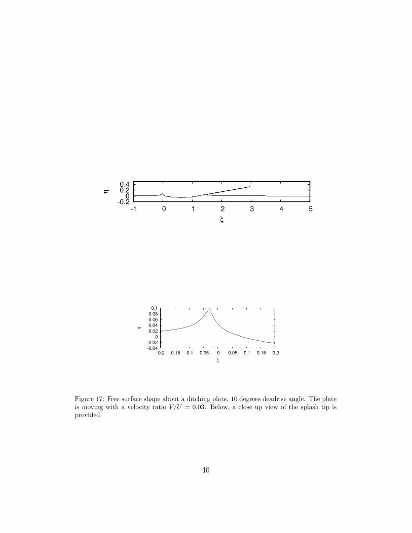
4.4. Ditching plate

As a last example, the solution method is applied to derive the self-similarsolution characterizing the water entry of a two-dimensional plate with ahigh horizontal velocity component, which is considered as an exemplificationof the aircraft ditching problem. There are two parameters governing thesolution in this case, which are the velocity ratio V/U and the angle γ formedby the plate with the still water level.

The problem is self-similar under following set of variables

ξ =x

Utη =

y

Utϕ =

φ

U2t, (62)

where U and V are the horizontal and vertical velocity of the plate. In termsof the variables (62), the plate edge is located at (1, V/U). The governingequations are about the same as (19)-(25), aside from the symmetry condi-tion, which does not hold in the ditching case. The boundary condition on

23

the body is

ϕν = sin γ +V

Ucos γ η = −V

U+ (ξ − 1) tan γ . (63)

As for the plate entry problem, also in this case an additional condition isenforced at the edge, requiring that the free surface is always attached tothe edge and that the free surface leave the plate tangentially. The solutionon the left hand side is then rather similar to that of the plate entry case,with the dynamic boundary condition changing the sign at some inversionpoint. The position of the inversion point is determined by enforcing the twoadditional conditions at the plate edge.

In Fig. 17 the solution is shown in terms of free surface shape for a platewith γ = 10 degrees and a velocity ratio V/U = 0.03. The solution displaysthe very thin jet developing along the plate. According to the definition ofthe stretched variables (62), the tip of the jet moves with a velocity whichis about three times the velocity of the plate. With similar considerations,the root of the jet, which is just in front of the pressure peak, moves witha horizontal velocity which is about 1.5 times the horizontal velocity of theplate.

Beside the thin jet developing along the plate, a splash is formed at therear. Differently from that found for the vertical entry case, the splash ismuch milder and much thicker, with a rather large angle formed by the twosides of the free surface at the tip. For the case presented here, the tip of thesplash is located at (−0.029, 0.099), and the free surface is inclined of about52 and 67 degrees with respect to the still water level on the left and righthand side, respectively. This result in an internal angle of about 61 degrees.

The pressure distribution for the same case is plotted in Fig. 18, whereψ = p/(%U2). The pressure peak is located at ξ ' 1.49, and thus the distanceto the plate edge is 0.49/ cos 10 ' 0.4976. In the physical variables this meansthat in a frame of reference attached to the body, the peak moves along thebody surface with a velocity equal to 0.4976U .

Another important information that can be derived by the pressure dis-tribution is the total hydrodynamic load acting on the plate. By integratingthe pressure distribution it is obtained that

F =

∫pds = (%U3t)

∫ψdτ

where τ is the arclength measured along the body in the self-similar plane.

24

From the numerical integration of the pressure distribution along the wettedsurface it is obtained that F ' 0.156(%U3t).

5. Conclusions

An iterative method for the solution of the fully nonlinear boundary valueproblems characterizing self-similar free surface flows has been presented.The method has been applied to different examples characterized by differentboundary conditions in order to demonstrate the good level of flexibility andaccuracy. It has been shown that the method keeps a good accuracy evenwhen dealing with the thin jets developing during water entry processes. Inthis regard, the shallow water model proved to be very efficient, thus allowinga significant reduction of the computational effort without reducing the levelof accuracy.

The applications presented here are all referred to constant velocity. Fu-ture extension of the method may involve constant acceleration cases, as thatdiscussed in Needham et al. (2008). In those cases however, additional andmore stringent hyphotheses are needed in order to guarantee that gravityand surface tension effects are still negligible.

Acknowledgement

The author wish to thank Prof. Alexander Korobkin for the useful discus-sions had during the development of the mathematical model and algorithm.The part about the ditching problem has been done within the SMAES-FP7project (Grant Agreement N. 266172)

References

Battistin, D. & Iafrati, A. 2003 Hydrodynamic loads during water entry oftwo- dimensional and axisymmetric bodies, J. Fluid Struct. 17, 643664.doi:10.1016/S0889-9746(03)00010-0

Battistin, D. & Iafrati, A. 2004 A numerical model for the jetflow generated by water impact, J. Engng. Math. 48, 353-374. doi:10.1023/B:engi.0000018173.66342.9f

Dobrovol’skaya, Z.N. 1969 On some problems of similarity flow of fluid witha free surface, J. Fluid Mech. 36, 805-829. doi:10.1017/S0022112069001996

25

Faltinsen, O.M. & Semenov, Y.A. 2008 Nonlinear problem of flat-plateentry into an incompressible liquid, J. Fluid Mech. 611, 151-173.doi:10.1017/S0022112008002735

Iafrati, A. & Battistin, D. 2003 Hydrodynamics of water entry in presenceof flow separation from chines, Proc. 8th Int. Conf. Num. Ship Hydrod.,Busan, Korea.

Iafrati, A. & Korobkin, A.A. 2004 Initial stage of flat plate impact onto liquidfree surface, Phys. Fluids 16, 2214-2227. doi:10.1063/1.1714667

Iafrati, A. & Korobkin, A.A. 2005 Starting flow generated by the impulsivestart of a floating wedge, J. Engng. Math. 52, 99-126. doi:10.1007/s10665-004-3686-9

Iafrati, A. & Korobkin, A.A. 2005 Self-similar solutions forporous/perfotated wedge entry problem Proc. 20th IWWWFB (avail-able at www.iwwwfb.org), Spitzbergen, Norway.

Iafrati, A. 2007 Free surface flow generated by the water impact of a flat plate,Proc. 9th Int. Conf. Num. Ship Hydrod., Ann Arbor (MI), USA.

Iafrati, A., Miloh, T. & Korobkin, A.A. 2007 Water entry of a block slidingalong a sloping beach, Proc. Int. Conf. Violent Flows (VF-2007), Fukuoka,Japan.

Iafrati, A. & Korobkin, A.A. 2008 Hydrodynamic loads during earlystage of flat plate impact onto water surface, Phys. Fluids 20, 082104.doi:10.1063/1.2970776

Iafrati, A. & Korobkin, A.A. 2011 Asymptotic estimates of hydrodynamicloads in the early stage of water entry of a circular disk, J. Engng. Math.69, 199-224. doi:10.1007/s10665-010-9411-y

King, A.C. % Needham, D.J. 1994 The initial development of a jet caused byfluid, body and free-surface interaction. Part 1. A uniformly acceleratingplate, J. Fluid Mech. 268, 89-101. doi:10.1017/S0022112094001278

Korobkin, A.A & Pukhnachov, V.V. 1988 Initial Stage of Water Impact, Ann.Rev. Fluid Mech. 20, 159-185. doi: 10.1146/annurev.fl.20.010188.001111

26

Korobkin, A.A. & Iafrati, A. 2006 Numerical study of jet flow gener-ated by impact on weakly compressible liquid, Phys. Fluids 18, 032108.doi:10.1063/1.2182003

Mei, X., Liu, Y. & Yue, D.K.P. 1999 On the water impact of generaltwo-dimensional sections, App. Oc. Res. 21, 1-15. doi:10.1016/S0141-1187(98)00034-0

Molin, B. & Korobkin, A.A. 2001 Water entry of a perforated wedge, Proc.16th IWWWFB (available at www.iwwwfb.org), Hiroshima, Japan.

Needham, D.J., Billingham, J. & King, A.C. 2007 The initial de-velopment of a jet caused by fluid, body and free-surface interac-tion. Part 2. An impulsively moved plate, J. Fluid Mech. 578, 67-84.doi:10.1017/S0022112007004983

Needham, D.J., Chamberlain, P.G. & Billingham, J. 2008 The initial de-velopment of a jet caused by fluid, body and free surface interaction. part3. an inclined accelerating plate, Q. J. Mech. Appl. Math. 61, 581-614.doi:10.1093/qjmam/hbn019

Semenov, Y.A. & Iafrati, A. 2006 On the nonlinear water en-try problem of asymmetric wedges, J. Fluid Mech. 547, 231-256.doi:10.1017/S0022112005007329

Semenov, Y.A. & Yoon B.-S. 2009 Onset of flow separation for theoblique water impact of a wedge, Phys. Fluids 21, 112103 (11 pages).doi:10.1063/1.3261805

Xu, G.D., Duan, W.Y. & Wu, G.X. 2008 Numerical simulation of obliquewater entry of an asymmetrical wedge, Ocean Engng. 35, 1597-1603.doi:10.1016/j.oceaneng.2008.08.002

Xu, G.D., Duan, W.Y. & Wu, G.X. 2010 Simulation of water entry of awedge through free fall in three degrees of freedom, Proc. R. Soc. A 466,2219-2239. doi:10.1098/rspa.2009.0614

Yakimov, Y.L. 1973 Influence of atmosphere at falling of bodies on water Izv.Akad. Nauk SSSR, Mekh. Zhidk. 5, 3-7.

27

Wu, G.X., Sun, H. & He, Y.S. 2004 Numerical simulation and experimentalstudy of water entry of a wedge in free fall motion, J. Fluids Struct. 19,277-289. doi:10.1016/j.jfluidstructs.2004.01.001

Zhao, R. & Faltinsen, O.M. 1993 Water entry of two-dimensional bodies, J.Fluid Mech. 246, 593-612. doi:10.1017/S002211209300028X

28

SB

SF

SS

η

ξρ

τ

Figure 1: Sketch of the computational domain and of the notation adopted.

Sν=0Sν<0

ν

Figure 2: Orientation of the normal velocity field on the free surface guess.

τ

µ

λ λ λi+1 i

µ=f ( )λ

Figure 3: Model adopted for the thin jet and local coordinate system for the shallow watermodel.

29

-0.2

0

0.2

0.4

0.6

0.8

6 6.5 7 7.5 8 8.5 9

η

ξ

0.1

0.2

0.3

0.4

0.5

0.6

8 8.2 8.4 8.6 8.8 9 9.2 9.4

η

ξ

Figure 4: Convergence of the iterative process for a wedge with 10 degrees deadrise angle.The left picture display the early stage of the process, starting from the initial configura-tion, till the formation of the thin jet layer (not shown) where the shallow water model isadopted. On the right picture, the convergence process about the root of the jet is shown.

0

5

10

15

20

25

30

35

40

0 2 4 6 8 10

ψ

ξ

0

5

10

15

20

25

30

35

40

8 8.2 8.4 8.6 8.8 9 9.2

ψ

ξ

Figure 5: Convergence of the pressure distribution for the 10 degrees wedge. A close upview of the pressure about the jet root is shown, displaying a smooth transition to zerothanks to the use of the shallow water model.

30

0.0001

0.001

0.01

0.1

1

10

0 10000 20000 30000 40000

K

Its

Figure 6: Convergence history of the kinematic boundary condition. The curves refer totwo different discretizations, the coarser having a minimum panel size of 0.04, the finer0.01.

31

-2-1 0 1 2 3

0 5 10 15 20 25 30 35 40

η

ξ

-2

-1.5

-1

-0.5

0

0.5

1

1.5

2

0 1 2 3 4 5

η

ξ

Figure 7: Comparison between the free surface profiles. In the upper picture, solutions re-fer to 5, 7.5, 10, 20 degrees deadrise angle. In lower picture, solution refer to 30, 40, 50, 60, 70and 80 degrees deadrise angle.

32

0

5

10

15

20

25

30

35

40

0 10 20 30 40 50 60 70 80

l j

γ

1

10

10

l j

γ

Figure 8: Distance of the jet tip to the wedge apex, versus the wedge angle. Accordingto the definition of self-similar variables (9), ljV represents the velocity at which the tipswept the body surface. The dash line represent the C/γ line, where C = 190 if the angleis expressed in degrees. The graph is given in logscale on the right.

0

20

40

60

80

100

120

140

160

0 5 10 15 20

ψ

ξ

0

0.5

1

1.5

2

2.5

3

3.5

0 0.5 1 1.5 2 2.5 3 3.5 4

ψ

ξ

Figure 9: Comparison between the pressure distributions. Solutions for 5, 7.5, 10, 20 de-grees deadrise angle are shown on the left, whereas solutions for 30, 40, 50, 60, 70 and 80degrees deadrise angle are given on the right.

33

-1

-0.5

0

0.5

1

1.5

2

2.5

0 2 4 6 8 10 12 14 16 18

η

ξ

0

5

10

15

20

25

30

35

40

0 2 4 6 8 10

ψξ

Figure 10: Effect of the porosity on the free surface shape and pressure distribution.Solutions are drawn for deadrise angle γ = 10 degree, with porosity coefficients α0 = 0, 0.02and 0.05.

0

0.5

1

1.5

2

1.5 2 2.5 3 3.5 4 4.5 5

η

ξ

0

0.5

1

1.5

2

2.5

3

3.5

0 0.5 1 1.5 2 2.5 3 3.5

ψ

ξ

Figure 11: Free surface shapes and pressure distributions for a wedge γ = 30 de-grees deadrise angle in case of perforated surfaces. The perforated coefficients are0, 0.02, 0.05, 0.10, 0.20, 0.30, 0.40, 0.50.

34

SF

SW

SB

V

O

η

A

γ

θ ξ

Figure 12: Block sliding along an inclined sloping bed.

35

-1

-0.5

0

0.5

1

1.5

2

0 0.5 1 1.5 2 2.5

η

ξ

-1

-0.5

0

0.5

1

1.5

0 0.5 1 1.5 2 2.5

η

ξ

-1

-0.5

0

0.5

1

1.5

0 0.5 1 1.5 2 2.5

η

ξ

Figure 13: Free surface profiles for a block, 60 degrees (top), 90 degrees (middle), 120degrees (bottom). Solutions are drawn for bed slopes 10, 20, 30, 40 and 50 degrees. Theline about the jet root indicates the position where the shallow water model is started.

36

0

0.2

0.4

0.6

0.8

1

1.2

1.4

0.5 1 1.5 2 2.5

η

ξ

Figure 14: Effect of the permeability of the front on the free surface elevation. Solutionsrefer to a block front 90 degrees inclination, with χ = 0 (solid), χ = 0.1 (dash) and χ = 0.2(dot).

37

0

0.5

1

1.5

2

0 0.2 0.4 0.6 0.8 1

η

ξ

0

0.5

1

1.5

2

0 0.4 0.8 1.2 1.6

η

ξ

Figure 15: On the left, the convergence history of the free surface shape nearby the plateedge is shown. On right, the final solution is compared to the experimental data byYakimov (1973).

38

0

0.05

0.1

0.15

0.2

0.25

0.3

0.35

0.4

-20 -15 -10 -5 0

ψ

ξ

Figure 16: Pressure distribution acting on the plate.

39

-0.2 0

0.2 0.4

-1 0 1 2 3 4 5

η

ξ

-0.04

-0.02

0

0.02

0.04

0.06

0.08

0.1

-0.2 -0.15 -0.1 -0.05 0 0.05 0.1 0.15 0.2

η

ξ

Figure 17: Free surface shape about a ditching plate, 10 degrees deadrise angle. The plateis moving with a velocity ratio V/U = 0.03. Below, a close up view of the splash tip isprovided.

40

0

0.2

0.4

0.6

0.8

1

1.2

1 1.1 1.2 1.3 1.4 1.5 1.6 1.7 1.8

ψ

ξ

Figure 18: Pressure distribution about a ditching plate, 10 degrees deadrise angle, withvelocity ratio V/U = 0.03.

41