Iterative ARIMA-Multiple Support Vector Regression models for long term time series prediction Jo˜ ao Fausto Lorenzato de Oliveira and Teresa B. Ludermir * Federal University of Pernambuco - Center of informatics Av. Jornalista Anibal Fernandes, s/n, Recife, PE, 50.740-560, Brazil Abstract. Support Vector Regression (SVR) has been widely applied in time series forecasting. Considering long term predictions, iterative predic- tions perform many one-step-ahead predictions until the desired horizon is achieved. This process accumulates the error from previous predictions and may affect the quality of forecasts. In order to improve long term iterative predictions a hybrid multiple Autoregressive Integrated Moving Average(ARIMA)-SVR model is applied to perform predictions consider- ing linear and non-linear components from the time series. The results show that the proposed method produces more accurate predictions in the long term context. 1 Introduction A time series is a discrete-time stochastic process composed by a finite set of items correlated in time. Time series forecasting has many applications in areas such as planning, management, production, maintenance and control of indus- trial processes. The forecasting process is based on some knowledge of the past, which can be performed by several statistical methods [1] and by nonlinear meth- ods such as Support Vector Regression (SVR) [2] and Artificial Neural Networks (ANNs) [3]. Some time series may present seasonal or\and trend patterns, which must be modeled by a method in order to produce better forecasts. Statistical methods such as ARIMA are able to map linear aspects such as trend, however nonlinear patterns are not easily captured. Different models can complement each other in capturing linear or nonlinear patterns of data sets in time series. Bates and Granger [4] explored several combinations of architectures for time series pre- diction, Pai and Lin used a hybrid ARIMA-SVR model to predict stock prices [5], Zhu and Wei used a hybrid ARIMA-Least Squares Support Vector Regres- sion(LSSVR) to predict carbon price. However, when performing iterative multi-step-ahead predictions, the accu- mulation of error may still be present at each forecast iteration. In order to address this problem, Zhang et al. used a multiple SVR [6] strategy where the SVR models are trained independently in different prediction horizons. This method reduces the number of iterations and may reduce the propagated error by performing many direct predictions. * The authors would like to thank FACEPE, CNPq and CAPES (Brazilian Research Agen- cies) for their financial support 207 ESANN 2014 proceedings, European Symposium on Artificial Neural Networks, Computational Intelligence and Machine Learning. Bruges (Belgium), 23-25 April 2014, i6doc.com publ., ISBN 978-287419095-7. Available from http://www.i6doc.com/fr/livre/?GCOI=28001100432440.
Transcript
Iterative ARIMA-Multiple Support VectorRegression models for long term time series
prediction
Joao Fausto Lorenzato de Oliveira and Teresa B. Ludermir ∗
Federal University of Pernambuco - Center of informaticsAv. Jornalista Anibal Fernandes, s/n, Recife, PE, 50.740-560, Brazil
Abstract. Support Vector Regression (SVR) has been widely applied intime series forecasting. Considering long term predictions, iterative predic-tions perform many one-step-ahead predictions until the desired horizonis achieved. This process accumulates the error from previous predictionsand may affect the quality of forecasts. In order to improve long termiterative predictions a hybrid multiple Autoregressive Integrated MovingAverage(ARIMA)-SVR model is applied to perform predictions consider-ing linear and non-linear components from the time series. The resultsshow that the proposed method produces more accurate predictions in thelong term context.
1 Introduction
A time series is a discrete-time stochastic process composed by a finite set ofitems correlated in time. Time series forecasting has many applications in areassuch as planning, management, production, maintenance and control of indus-trial processes. The forecasting process is based on some knowledge of the past,which can be performed by several statistical methods [1] and by nonlinear meth-ods such as Support Vector Regression (SVR) [2] and Artificial Neural Networks(ANNs) [3].
Some time series may present seasonal or\and trend patterns, which must bemodeled by a method in order to produce better forecasts. Statistical methodssuch as ARIMA are able to map linear aspects such as trend, however nonlinearpatterns are not easily captured. Different models can complement each otherin capturing linear or nonlinear patterns of data sets in time series. Bates andGranger [4] explored several combinations of architectures for time series pre-diction, Pai and Lin used a hybrid ARIMA-SVR model to predict stock prices[5], Zhu and Wei used a hybrid ARIMA-Least Squares Support Vector Regres-sion(LSSVR) to predict carbon price.
However, when performing iterative multi-step-ahead predictions, the accu-mulation of error may still be present at each forecast iteration. In order toaddress this problem, Zhang et al. used a multiple SVR [6] strategy where theSVR models are trained independently in different prediction horizons. Thismethod reduces the number of iterations and may reduce the propagated errorby performing many direct predictions.
∗The authors would like to thank FACEPE, CNPq and CAPES (Brazilian Research Agen-cies) for their financial support
207
ESANN 2014 proceedings, European Symposium on Artificial Neural Networks, Computational Intelligence and Machine Learning. Bruges (Belgium), 23-25 April 2014, i6doc.com publ., ISBN 978-287419095-7. Available from http://www.i6doc.com/fr/livre/?GCOI=28001100432440.
In this paper we propose a Multiple ARIMA-SVR model in order to maplinear and nonlinear patterns in time series and to improve the accuracy initerative long term forecasts. The remainder of this paper is organized as follows:Section 2 presents a brief review of time series forecasting strategies, Section3 shows the proposed method. Section 4 presents the experiments and theconclusions and future works are presented in section 5.
2 Time series forecasting
In this section, the iterated, direct and multiple approaches for time series fore-casting are reviewed. For all three approaches consider a time series {zt}Nt=1,where N is the length of the time series.
In the one-step-ahead prediction the model depends on the d past valuesand has the form z′(t + 1) = f(z(t), z(t − 1), ..., z(t − (d − 1))), where d is theembedding dimension or time window.
The prediction of p-steps-ahead in the iterative approach takes the formz′(t + h) = f(z′(t + h − 1), z′(t + h − 2), ..., z′(t + h − d)) [7], where the past dpredictions are taken into consideration in order to perform the pth prediction.In the iterative approach, the model is trained to perform one-step-ahead pre-dictions at time t+1 iteratively h times using past predictions as inputs for thenext prediction. This process do not need information at the desired horizon hhowever it accumulates the error from all the past predictions. Only one modelis required to perform predictions.
The prediction of p-steps-ahead in the direct approach has the form z′(t +h) = f(z(t), z(t− 1), ..., z(t− (d− 1))) [8]. In other words, the model is traineddirectly at the horizon h, and the predictions are performed directly into thathorizon. In this approach we need information at horizon h in order to trainthe model and the error is not accumulated. To perform predictions in differentvalues of h, other models have to be trained at this horizon.
The multiple approach takes into consideration the iterative and direct meth-ods [6]. Multiple models are trained independently at different horizons, and per-form iterative predictions until the desired horizon is achieved. Given a horizonh, k models (with k < h) will be trained independently to perform predictionsat the horizons {t + 1, t + 2, ..., t + k}. This method does not need to train hmodels as needed in the direct approach and produces less accumulation of errorthan the iterative method.
3 Proposed Method
The proposed method incorporates the linear and nonlinear mappings of the timeseries through a composition of a ARIMA model and multiple SVR models.
The ARIMA model was first introduced by Box and Jenkins [9] and has beenwidely applied in time series forecasting. The predictions in the ARIMA modelare a linear combination of past values and past residual errors, and has theform presented on eq. 1.
208
ESANN 2014 proceedings, European Symposium on Artificial Neural Networks, Computational Intelligence and Machine Learning. Bruges (Belgium), 23-25 April 2014, i6doc.com publ., ISBN 978-287419095-7. Available from http://www.i6doc.com/fr/livre/?GCOI=28001100432440.
θp(B)(1−B)szt = ϕq(B)ϵt (1)
where zt is the actual value and ϵt is the residual error at time t, B is a backwardshift operator (Bzt = zt−1 and ∆zt = zt − zt−1 = (1 − B)zt), ϕi and θj arethe coefficients, p and q are degrees for the autoregressive and moving averagepolynomial functions. The integration part is due to the differencing performedto the time series in order to obtain a stationary series. The number of differencesis determined by the parameter s.
The SVR method was proposed by Vapnik [10] and it is based on the struc-tured risk minimization (SRM) principle, aiming at minimizing an upper bound
of the generalization error. Let {zi, yi}li=1 be a training set where z ∈ ℜd, yi ∈ ℜis the prediction output of zi, d is the embbeding dimension of the time seriesand l is the number of training samples. The objective of SVR is to find the bestfunction from a set of possible functions {f |f(z) = wT z + b, w ∈ ℜd, b ∈ ℜ},where w is the weight vector and b is a bias or threshold.
In order to find the best function f , it is necessary to minimize the regularizedrisk 1
2∥w∥2+ C
∑li=1 L(yi, f(zi)), where C > 0 is a regularization factor, ∥.∥ is
a 2-norm and L(., .) is a loss function. In order to induce sparsity in SVR theϵ-insensitive loss function presented on eq. 2, which creates an ϵ-tube allowingsome predictions to fall within the boundaries of this ϵ-tube.
L(y, f(z)) =
{0, |f(z)− y| < ϵ
|f(z)− y| − ϵ, otherwise(2)
The nonlinearity of SVRs is achieved by mapping the input space into ahigher dimensionality space. This mapping is possible through the use of kernels,and the regression function takes the form f(z) =
∑li=1 (αi − α∗
i )k(zi, z) + b,where α and α∗ are lagrange multipliers and k(zi, z) is a kernel function.
In this study, the gaussian kernel is adopted (k(zi, zj) = exp(−∥zi−zj∥2
2γ2 )),where γ is a parameter of the gaussian kernel.
The proposed model uses the ARIMA method as a prepossessing step inorder to map linear patterns in the time series.
z(t)z(t-1)
.
.
.z(t-d+1)
SVR 1
SVR 2
SVR k
.
.
.
.
.
e’(t+1)
e’(t+2)
e’(t+k)
SVR 1
SVR 2
SVR k
.
.
.
.
.
.
.
. . .
. . .
. . .
SVR 1
SVR 2
SVR k
z’(t+2).....
e’(t+(r-1)k+1)
e’(t+(r-1)k+2)
e’(t+(r-1)k+k)
ARIMA
e(t)e(t-1)
.
.
.e(t-d+1)
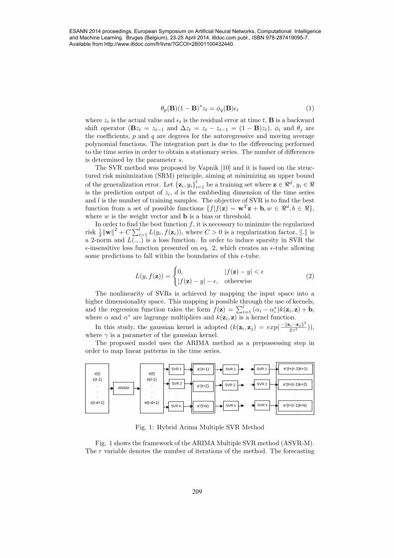
Fig. 1: Hybrid Arima Multiple SVR Method
Fig. 1 shows the framework of the ARIMAMultiple SVRmethod (ASVR-M).The r variable denotes the number of iterations of the method. The forecasting
209
ESANN 2014 proceedings, European Symposium on Artificial Neural Networks, Computational Intelligence and Machine Learning. Bruges (Belgium), 23-25 April 2014, i6doc.com publ., ISBN 978-287419095-7. Available from http://www.i6doc.com/fr/livre/?GCOI=28001100432440.
procedure of this method performs less iterations than the iterative method,which runs as many iterations as the horizon size.
The residuals produced by the ARIMA et = zt − z′t, are used as an inputfor the Multiple SVR methods. In this step, k SVR models are trained in-dependently, in order to perform iterative predictions. The final forecast canbe achieved by adding the forecasts of the ARIMA and multiple SVR modelso′t = z′t + e′t.
4 Experiments
The experiments were performed in four benchmark datasets including Sunspot,Airline Passengers, IBM stock prices and Death. Our proposed approach is com-pared with other methods such as Iterative SVR (SVR-I), Direct SVR (SVR-D),Multiple SVR (SVR-M), ARIMA Iterative SVR (ASVR-I) and ARIMA DirectSVR (ASVR-D), implemented using the LIBSVM package [11] in a MATLAB8.2 environment. The datasets were partitioned, using 80% for training and20% for testing. First the p, q and s parameters of the ARIMA(p,s,q) modelare defined with grid search 5-fold cross-validation in the training data withparameters ranging from {1, 2}, {0, 1, 2} and {0, 1, 2} respectively and the bestARIMA(p,s,q) model is selected based on the Aikake’s Information Criterion(AIC) [12].
In all SVR models the parameter selection was performed by doing a 10-foldcross-validation grid search in the residuals produced by the selected ARIMAmodel with C, ϵ and γ within the range {10−1, 100, 101, 102}, {10−4, 10−3, 10−2}and {2−5, 2−4, ..., 22} respectively on the training set according to [6].
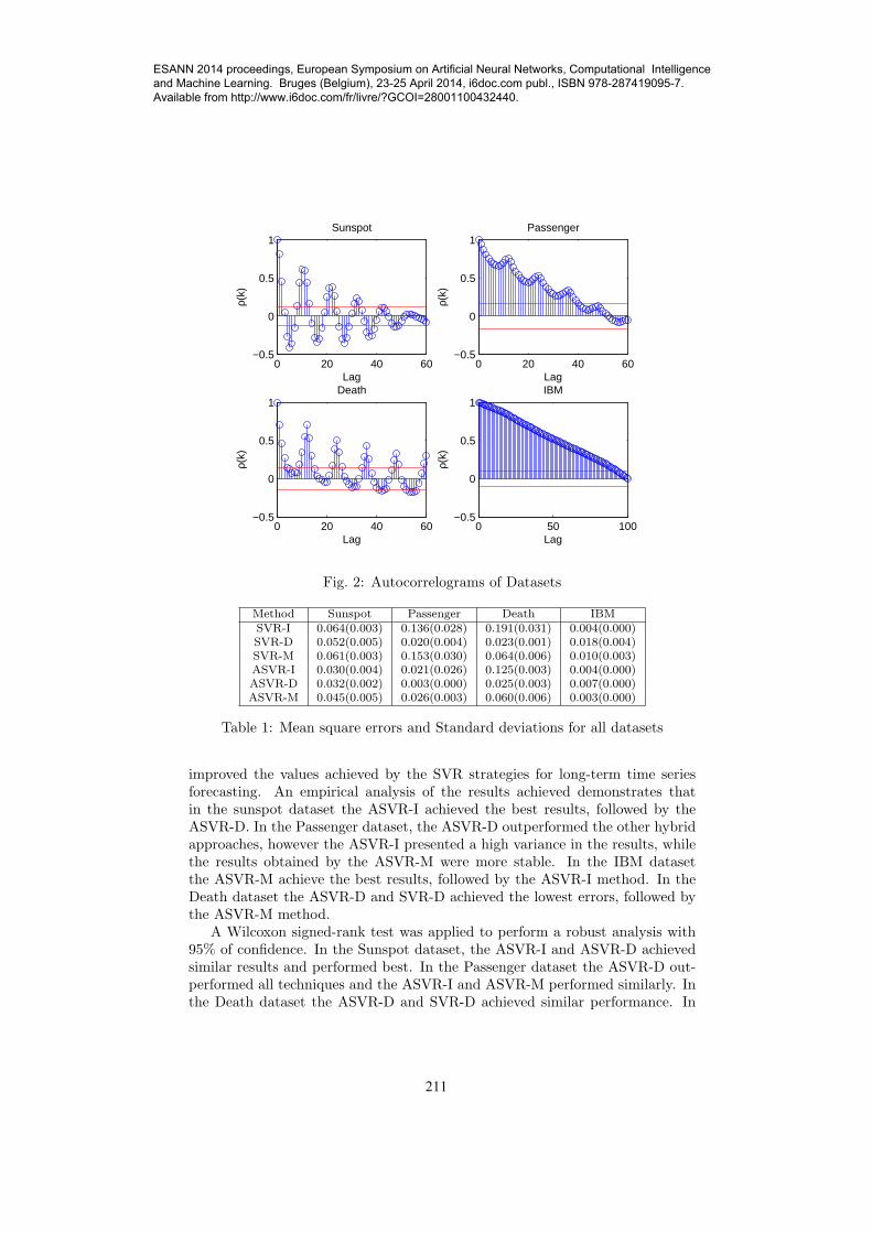
The annual Wolf’s sunspot numbers dataset has 289 points and presentsseasonal patterns. The monthly airline passengers dataset has 144 points andpresents trend and seasonal patterns. The death dataset represents the numberof deaths and serious injuries in UK road accidents each month and has 192points. The daily IBM stock closing prices has 369 points and presents trendpatterns. Fig 2 presents the autocorrelograms for all datasets, where the lagsare set to unity. The sunspot, passengers, IBM and death datasets are availablefrom [13].
The experiments for the sunspot, airlines passenger, death and IBM wereperformed considering an embedding dimension d = 6, prediction horizon h = 10and number of SVR models in the multiple approaches k = d based on [6]. Alldatasets had their values scaled to [0...1]. The experiments were executed for 10iterations.
The performance measure used in this work as the mean squared error (MSE)described on eq. 3.
MSE =
∑Ni=1 (zi − z′i)2
N(3)
Table 1 contemplates the mean and standard deviations for the MSEs in alldatasets. The results show that in most cases the hybrid ARIMA-SVR procedure
210
ESANN 2014 proceedings, European Symposium on Artificial Neural Networks, Computational Intelligence and Machine Learning. Bruges (Belgium), 23-25 April 2014, i6doc.com publ., ISBN 978-287419095-7. Available from http://www.i6doc.com/fr/livre/?GCOI=28001100432440.
Table 1: Mean square errors and Standard deviations for all datasets
improved the values achieved by the SVR strategies for long-term time seriesforecasting. An empirical analysis of the results achieved demonstrates thatin the sunspot dataset the ASVR-I achieved the best results, followed by theASVR-D. In the Passenger dataset, the ASVR-D outperformed the other hybridapproaches, however the ASVR-I presented a high variance in the results, whilethe results obtained by the ASVR-M were more stable. In the IBM datasetthe ASVR-M achieve the best results, followed by the ASVR-I method. In theDeath dataset the ASVR-D and SVR-D achieved the lowest errors, followed bythe ASVR-M method.
A Wilcoxon signed-rank test was applied to perform a robust analysis with95% of confidence. In the Sunspot dataset, the ASVR-I and ASVR-D achievedsimilar results and performed best. In the Passenger dataset the ASVR-D out-performed all techniques and the ASVR-I and ASVR-M performed similarly. Inthe Death dataset the ASVR-D and SVR-D achieved similar performance. In
211
ESANN 2014 proceedings, European Symposium on Artificial Neural Networks, Computational Intelligence and Machine Learning. Bruges (Belgium), 23-25 April 2014, i6doc.com publ., ISBN 978-287419095-7. Available from http://www.i6doc.com/fr/livre/?GCOI=28001100432440.
the IBM dataset the ASVR-M and SVR-I achieved similar results.
5 Conclusion
This paper realized a comparison between strategies (iterative, direct, multiple)to perform long-term time series forecasting using Support Vector Regression(SVR) models and proposed a hybrid model based on a Autoregressive IntegratedMoving Average (ARIMA) model and on multiple SVRs.
The direct approaches (SVR-D, ASVR-D) achieved the best results in mostdatasets, which is expected since there is no iterative error accumulation. How-ever the multiple approaches (SVR-M and ASVR-M) tends to reduce the accu-mulation error by running fewer iterations.
Under these settings the hybridization increased the performance of mostmethods, however the iterative method was the one with more increase of per-formance, in most cases achieving similar results to the ASVR-M.
For future works, we intend to analyze the performance of a hybridizationbetween ARIMA and an ensemble of SVRs to perform prediction using theiterative, direct and multiple strategies.
References
[1] Spyros Makridakis, Steven C Wheelwright, and Rob J Hyndman. Forecasting methodsand applications. Wiley. com, 2008.
[2] K-R Muller, Alex J Smola, Gunnar Ratsch, Bernhard Scholkopf, Jens Kohlmorgen, andVladimir Vapnik. Predicting time series with support vector machines. In ArtificialNeural Networks—ICANN’97, pages 999–1004. Springer, 1997.
[3] Guoqiang Zhang, B Eddy Patuwo, and Michael Y Hu. Forecasting with artificial neuralnetworks:: The state of the art. International journal of forecasting, 14(1):35–62, 1998.
[4] John M Bates and Clive WJ Granger. The combination of forecasts. OR, pages 451–468,1969.
[5] Ping-Feng Pai and Chih-Sheng Lin. A hybrid arima and support vector machines modelin stock price forecasting. Omega, 33(6):497–505, 2005.
[6] Li Zhang, Wei-Da Zhou, Pei-Chann Chang, Ji-Wen Yang, and Fan-Zhang Li. Iteratedtime series prediction with multiple support vector regression models. Neurocomputing,2012.
[7] Abdelhamid Bouchachia and Saliha Bouchachia. Ensemble learning for time series pre-diction. In Proceedings of the International Workshop on Nonlinear Dynamic Systemsand Synchronization, 2008.
[8] Souhaib Ben Taieb, Antti Sorjamaa, and Gianluca Bontempi. Multiple-output modelingfor multi-step-ahead time series forecasting. Neurocomputing, 73(10):1950–1957, 2010.
[9] George EP Box, Gwilym M Jenkins, and Gregory C Reinsel. Time series analysis:forecasting and control. Wiley. com, 2013.
[10] Vladimir Vapnik. The nature of statistical learning theory. springer, 2000.
[11] Chih-Chung Chang and Chih-Jen Lin. LIBSVM: A library for support vector machines.ACM Transactions on Intelligent Systems and Technology, 2:27:1–27:27, 2011.
[12] Hamparsum Bozdogan. Model selection and akaike’s information criterion (aic): Thegeneral theory and its analytical extensions. Psychometrika, 52(3):345–370, 1987.
[13] R.J. Hyndman. Time series data library, 2010.
212
ESANN 2014 proceedings, European Symposium on Artificial Neural Networks, Computational Intelligence and Machine Learning. Bruges (Belgium), 23-25 April 2014, i6doc.com publ., ISBN 978-287419095-7. Available from http://www.i6doc.com/fr/livre/?GCOI=28001100432440.