Journal of Computational Physics159,246–273 (2000)

doi:10.1006/jcph.2000.6435, available online at http://www.idealibrary.com on

An Iterative Grid Redistribution Method forSingular Problems in Multiple Dimensions

Weiqing Ren and Xiao-Ping Wang

Department of Mathematics, The Hong Kong University of Science and Technology,Clear Water Bay, Kowloon, Hong Kong

E-mail: mawang@ust.hk

Received September 1, 1999; revised December 13, 1999

We introduce an iterative grid redistribution method based on the variational ap-proach. The iterative procedure enables us to gain more precise control of the griddistribution near the regions of large solution variations. The method is particu-larly effective for solving partial differential equations with singular solutions (e.g.,blowup solutions). Our method requires little prior information of the singular so-lutions and can handle multiple singularities. The method is successfully applied tothe nonlinear Schr¨odinger equation and the Keller–Segal equations where solutionswith multiple blowup points can be solved up to times very close to the blowuptime. c© 2000 Academic Press

1. INTRODUCTION

Numerical solution of many problems from areas such as fluid dynamics, combustion, andheat transfer requires small node separations over a portion of the physical domain to resolvelarge solution variations. Using uniform meshes for these problems is formidable when thesystem involves two or more spatial dimensions. It is now widely recognized that an adaptivecomputation mesh increases the accuracy and decreases the cost of numerical calculations.Adaptivity is achieved in various ways by using, for example, local adaptive mesh refinement[2], moving finite elements mesh refinement [8, 13], adaptive node movement (see, e.g.,[3, 9, and references therein]), or methods based on attraction and repulsion pseudoforcesbetween nodes [14].

In this paper, we are mainly interested in adaptive mesh redistribution methods. Whensuch an adaptive method is used, the mesh point locations change while the solution ofthe physical problem is computed. Both the grid point locations and the original physicalunknowns evolve as part of the problem solution. The grid point movement is usuallyachieved in two different ways, static and dynamic. In a static method, mesh points areredistributed at fixed time levels according to a mesh generating rule. In a dynamic or moving

246

0021-9991/00 $35.00Copyright c© 2000 by Academic PressAll rights of reproduction in any form reserved.

ITERATIVE GRID REDISTRIBUTION 247

mesh method, the mesh points move continuously in the space–time domain according toa moving mesh equation. In both cases, the grid points are moved during the calculationin order to improve the quality of the result. This is usually assumed to mean that somemeasure of the total error in the solution has been reduced or physical resolution has beenimproved in regions where large changes in dependent variables occur.

The key ingredient of such adaptive methods is the grid generation rule. In grid generation,one seeks a change of independent variables (or a mapping from the physical domain tothe computational domain), such that, in the new variables, the variation of the concernedquantity (defined by the monitor function) is reduced. In the discrete level, this means thata uniform grid in the computational domain is mapped into the physical domain so thatmore grid points are concentrated in the regions of large variations. The question that weare concerned with in this paper is whether it is possible (and how) to determine an optimalcoordinate mapping in certain sense, so that we can achieve the best possible behavior inthe computation variables. As we will see later, this question is particularly important if theproblem that we are dealing with is singular.

In two (or higher) spatial dimensions, the commonly used mesh generation techniquesare based on a variational approach, many of which are derivations of a technique firstproposed by Winslow. The functional is chosen so that the minimum is suitably influencedby the solution of the partial differential equation (PDE). Specifically, given a solutionu(x)of the PDE at a fixed time, a mapping from the physical domainÄp to the computationaldomainÄc, which usually is taken to be the same asÄp,

ξ(x) : Äp→ Äc, (1.1)

is determined by minimizing a functional of the form

E(ξ) =∫Ä

1

w|∇ξ |2 dx, (1.2)

wherew(x) is a weight function (or monitor function) depending on the physical solutionu(x) to be adapted. The monitor function should be chosen so that the function in thecomputational domain given by

v(ξ) = u(x(ξ)) (1.3)

is better behaved. With (1.2), the coordinate transform (1.1) is determined from the Euler–Lagrange equation

∇ ·(

1

w∇ξ)= 0. (1.4)

In one dimension, (1.4) is simplified to

xξw = C, (1.5)

which is the differential form of the equidistribution rule used in many one-dimensionaladaptive methods [9].

Understanding how the monitor function influences the resulting mesh properties iscrucial for the success of a mesh adaption method. In one dimension, such a relation is

248 REN AND WANG

given by the equidistribution rule, but only in an average sense. In multiple dimensions, it iseven more difficult to predict the overall resulting mesh behavior from the monitor functionitself. In other words, it is difficult to have a precise control of the resulting grid distributionfrom (1.4) or (1.5). Our numerical experiments using the above methods in various formshave shown that adaptivity is achieved only when the solution is moderate. However, gridpoints stop moving toward (or even turn away from) the singular region when singularityis approached; i.e., adaptivity is lost when it is most needed. Part of the reason is becausethe solution is so concentrated in a small region that it has little effect on the grids faraway from the singularity. An explicit reason for the failure is given in Section 3 for theone-dimensional problem. In a particular application, such a problem may be fixed partiallyby choosing a carefully designed monitor function when the structure of the singularity isavailable. But a method that works in general is desirable. Such a method must be based ona better grid redistribution procedure than those given above.

In Section 4, we introduce an iterative grid redistribution method. The fundamental ideais that one realizes that a successive application of the mapping (the Winslow mapping)obtained from (1.1)–(1.4) (or the generalization of them) improves the adaptivity of thegrids. In fact, our results indicate that the iteration converges to an optimal coordinatemapping in the sense that the monitor function converges to a constant function almosteverywhere. With the iteration procedure, we gain control of the mesh distribution near thesingular point; i.e., we may achieve desirable grid adaption by controlling the number ofmesh iterations. In Section 5, we show how our iterative grid redistribution procedure canbe easily implemented in a static adaptive grid redistribution procedure for PDEs.

In Section 6, we show several numerical examples. We mainly apply our method tothe nonlinear Schr¨odinger equation [11, 12]. The dynamic rescaling method has been avery successful method for solving the blowup solutions of the nonlinear Schr¨odingerequation (NLS). Not only it can integrate the equation very close to blowup time, themethod also provides the blowup profile as well as the rate of blowup. However, the methodis restricted to the case in which the solution blows up at only a single point and it alsocannot resolve the solution outside the self-similarity region. In our numerical examples,we will demonstrate the capability of our method for tracking multiple singularities. First,we solve the nonlinear Schr¨odinger equation with a single blowup point and the results areshown to match the results obtained by the dynamic rescaling method. More importantly,in the second example we solve a solution that blows up at two points. To the best of ourknowledge, such calculations have never been done before, at least not with such highresolutions. We also show a calculation in a supercritical case where the boundary of theregion of self-similarity can be determined by our method. This shows that not only ourmethod can resolve the singular regions, it also takes care of the the regions away fromthe singularities. Finally, we will show a numerical solution for the Keller–Segal modelfor bacterial pattern formation where multiple singularities arise from an initial uniformbacterial density distribution.

Note that various improvements of Winslow’s method have been considered by manyauthors [1, 3, 4, 10, 14, 17]. For example, Brackbill [4] incorporates an efficient directionalcontrol as well as orthogonality of the mesh into the mesh adaption by adding to (1.2) morefunctionals measuring those effects and thereby improves both accuracy and efficiency incertain physical problems. Further improvement can also be obtained by introducing a “gridinertia” term into the formulation (see [17]). It is expected that our iterative procedure canalso be applied in a similar way to problems where directional control and orthogonality of

ITERATIVE GRID REDISTRIBUTION 249

the mesh are important. We also note that, in this paper, we do not consider the effect of gridsmoothing which is important in many applications, especially when solution (singular)structure is complex.

2. VARIOUS GRID GENERATION RULES

2.1. Grid Distribution Based on the Equidistribution Principle in One Dimension

The equidistribution principle was introduced by de Boor [7] for solving boundary valueproblems for ordinary differential equations. It involves selecting mesh points such that somemeasure of the solution error is equalized over each subinterval. Based on this principle,many moving mesh methods have been developed.

Let x andξ denote the physical and computational coordinates, respectively, on the unitinterval [0, 1]. A one-to-one coordinate transformation between these domains is denotedby {

x = x(ξ), ξ ∈ [0, 1]

x(0) = 0, x(1) = 1.(2.1)

Suppose that a uniform mesh is given on the computational domain by

ξi = i

n, i = 0, 1, . . . ,n,

where n is a certain positive integer, and denote the corresponding mesh inx by{x0, x1, . . . , xn}. For a chosen monitor functionw(x) (>0), which provides some mea-sure of the computational error in the solutionu(x) of the underlying physical PDE, the(one-dimensional) equidistribution principle can be expressed in its integral form as∫ x

0w(s) ds= ξC, (2.2)

where

C =∫ 1

0w(s) ds, (2.3)

or equivalently, in the discrete form,∫ xi+1

xi

w(x) dx =∫ xi

xi−1

w(x) dx for i = 1, 2, . . . ,n− 1.

Differentiating (2.2) once, we obtain a differential form,

w(x(ξ))∂

∂ξx(ξ) = C. (2.4)

Whenw(x)=√1+ u2x, the above method is known as the “arclength method.”

250 REN AND WANG

2.2. Grid Distribution Based on the Variational Principle

The above equidistribution principles cannot be generalized directly to two or higherdimensions. In fact, equidistribution can be achieved locally in only a certain way [9].In two (or higher) spatial dimensions, mesh adaption is commonly done using the varia-tional approach, specifically by minimizing a functional of the coordinate mapping betweenthe physical domain and the computational domain. The functional is chosen so that theminimum is suitably influenced by the desired properties of the solution of the PDE itself.

Again, letx andξ denote the physical and computational coordinates, respectively, on adomainÄ ∈ Rd. A one-to-one coordinate transformation onÄ is denoted by

x = x(ξ), ξ ∈ Ä. (2.5)

The functionals used in existing variational approaches for mesh generation and adaptationcan usually be expressed in the form

E(ξ) =∫Ä

∑i, j,α,β

gi, j ∂ξα

∂xi

∂ξβ

∂x jdx, (2.6)

whereG= (gi, j ),G−1= (gi, j ) are symmetric positive definite matrices that are monitorfunctions in a matrix form. The coordinate transformation and the mesh are determinedfrom the Euler–Lagrange equation,

∇ · (G−1∇ξ) = 0. (2.7)

Equations (2.6) and (2.7) are related to the theory of the harmonic map, where the Hamilton–Schoen–Yau theorem guarantees the existence and uniqueness of the mapping with nonva-nishing Jacobian.

We note that more terms can be added to the functional (2.6) to control other propertiesof the mesh, such as orthogonality of the mesh and the alignment of the mesh lines with aprescribed vector field [4].

2.3. Winslow’s Variable Diffusion Equation

A special case of (2.6) is Winslow’s variable diffusion method. Winslow [16] suggesteda functional of the form

E(ξ) =∫Ä

∑j

1

w|∇ξ j |2 dx, (2.8)

wherew>0 is a weight function depending on the physical solution to be adapted, and thiscorresponds to (2.6) with the monitor function,

G = w I .

The Euler–Lagrange equations whose solution minimizesE are

∇ · 1

w∇ξ j = 0, (2.9)

which are diffusion equations.

ITERATIVE GRID REDISTRIBUTION 251

The diffusion coefficientD= 1w

can be directly related to the cell area or volume [1]. Wedenote the Jacobian of the mapping as defined as

J∗ = ξxηy − ξyηx

for the two-dimensional case. Let̄D= ln D, J̄=−ln J∗. A straightforward calculationgives

∇2(J̄ − D̄

)−∇ J̄ · ∇( J̄ − D̄) = −R J∗−1,

where

R= 2

[∇(∂ξ

∂x

)· ∇(∂η

∂y

)−∇

(∂ξ

∂y

)· ∇(∂η

∂x

)].

If we assume the term on the right side,R J∗−1, to be small, then we have

∇2( J̄ − D̄)−∇ J̄ · ∇( J̄ − D̄) = 0

and a solution may readily be written as

∇( J̄ − D̄) = 0

or

( J̄ − D̄) = constant (2.10)

and

DJ∗ = C,

whereC is a constant. This shows thatD is proportional to theJ∗−1. Therefore, equidistri-bution is approximately satisfied in the regions whereR J∗−1 is small.

2.4. Solving the Generator Equation by Heat Flow

In our applications, the solutions of the elliptic system (2.9) are obtained as a steady stateof the heat flow equations [10],{

∂ξ

∂t −∇ ·(

1w∇ξ) = 0

∂η

∂t −∇ ·(

1w∇η) = 0.

(2.11)

That is, we solve the evolution Eq. (2.11) for long time until the solution becomes almoststeady. This steady state is used as the solution to (2.9). Note thatt in (2.11) should notbe confused with the time variablet used in the underline nonlinear PDE (5.1). For actualcomputation, the dependent and independent variables in (2.11) are interchanged and wehave

xt = −xξJ

{∂

∂ξ

(xTη

1

Jwxη

)− ∂

∂η

(xTξ

1

Jwxη

)}− xη

J

{∂

∂ξ

(xTη

1

Jwxξ

)+ ∂

∂η

(xTξ

1

Jwxξ

)}, (2.12)

252 REN AND WANG

where the JacobianJ= xξ yη−xηyξ . The steady-state solution of (2.12) serves as the desiredsolution of (2.9). We can start from a uniform mesh, i.e.,x(ξ, η,0)= ξ, y(ξ, η,0)= η, orfrom an appropriate initial guess provided in the problem.

It is obvious that, to improve efficiency, more sophisticated elliptic solvers, such as themultigrid method, can be used to solve the elliptic system. In our method, grid redistributionwere needed only once in a while. Computational cost for this part is not an issue (at leastin two dimensions).

3. PROPERTIES OF THE RESULTING GRID DISTRIBUTION

IN THE EXTREME CASE

From equidistribution property in one dimension and the properties of the solution of theWinslow equations, we expect more grid points will be concentrated at the regions of rapidvariation of the solution. However, we will show that when the solution becomes singular,such grid adaptivity is actually lost with the above methods.

3.1. Numerical Tests

We first consider a one-dimensional example. Let

u(x) = 1

εe−(

x−0.5ε )

2

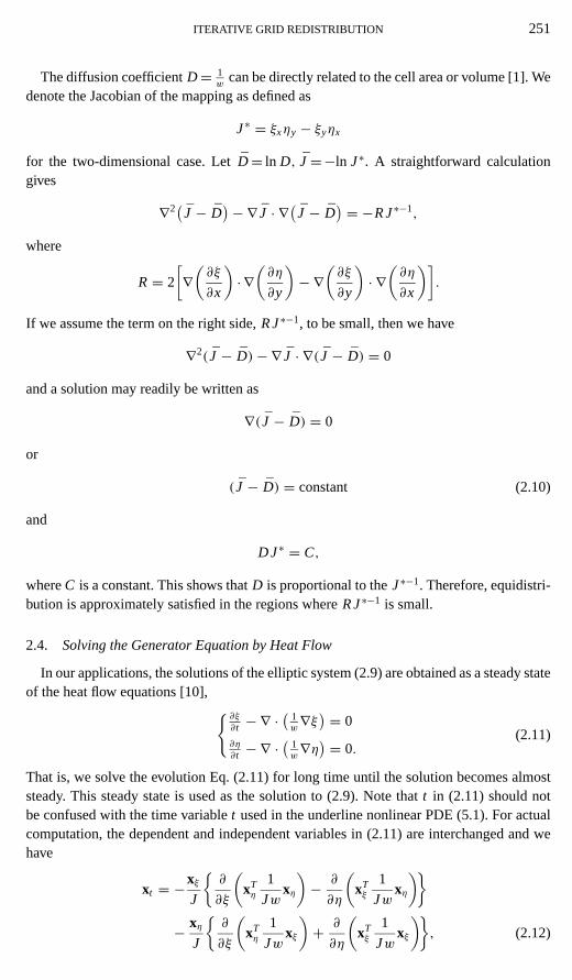
and the monitor function bew=√1+ u. We show the grid distribution for variousε inFig. 1. It is clear from the graph that as one decreasesε, the grid points move toward thecenter first, but most of the points then move away from the center asε continues to decrease.

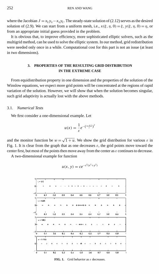
A two-dimensional example for function

u(x, y) = ce−c2(x2+y2)

FIG. 1. Grid behavior asε decreases.

ITERATIVE GRID REDISTRIBUTION 253

FIG. 2. Grid behavior foru= ce−c2(x2+y2) in 2-d asc increases.

shows similar grid behavior. Figure 2 shows the grid distributions obtained from (2.9) fortwo different monitor functions

(a) w(x, y) =√

1+ |u|2, (b) w(x, y) =√

1+ |∇u|2.

In both cases, we see that, just like in one dimension, grid adaption is achieved for smallerc and then lost whenc is large.

Other examples with various choices of monitor functions exhibit similar phenomena.Such behavior seems to be generic when the monitor function becomes singular.

254 REN AND WANG

3.2. Asymptotic Analysis

To understand the above phenomena, let’s assume that we have a monitor function thatis close to a self-similar singularity characterized by a parameterε,

wε(x) =√

1+ 1

εkg(x

ε

),

whereg(y) is positive, has maximum atx= 0, and decays rapidly (say, faster than1yn for a

large enoughn) asy→∞. We want to study the behavior of the grid asε→ 0. From (2.4),we have

xξ = C(ε)

w= C(ε)√

1+ 1εk g(

xε

) , (3.1)

where

C(ε) =∫ 1

0

√1+ 1

εkg(x

ε

)dx.

Integration by parts, we have

C(ε) = x

√1+ 1

εkg(x

ε

)∣∣∣∣10

−∫ 1

0

x 1εk g′(x)

2√

1+ 1εk g(

xε

) dx

=√

1+ 1

εkg(x

ε

)− ε1− k

2

∫ 1ε

0

yg′(y)

2√εk + g(y)

dy.

Sinceg(y) decays rapidly asy→∞, we have, asε→ 0,

C(ε) ∼ 1+ Aε1− k2 , (3.2)

where

A = −∫ ∞

0

yg′(y)2√

g(y)dy=

∫ ∞0

√g(y) dy.

We thus have forx 6= 0 (i.e., away from the singularity) andε→ 0

xξ → 1 when k < 2

xξ → 1+ A when k = 2 (3.3)

xξ →∞ when k > 2.

This implies that, in the casek < 2, we have1X=1ξ away from the singularity. Therefore,asε→ 0, only grid points very close to 0 are allowed to move; i.e., the grid adaption is verylimited near the place that functiong is large. This also shows that one has to know thesolution behavior in some detail in order to design the monitor function which can generatethe desired grid distribution near the singularity.

ITERATIVE GRID REDISTRIBUTION 255

4. AN ITERATIVE REMESHING PROCEDURE

To improve the mesh adaption, we introduce an iterative remeshing procedure. Let usfirst define the Winslow mapping:

T: (x, u(x))→ (ξ, v(ξ)).

Herex= x(ξ) is determined from (2.9), where the monitor functionw(x) depends onu(x);v(ξ)= u(x(ξ )).

If the monitor functionw is chosen properly, the resulting mesh should concentrate moregrid points in the regions with large variations. This also means thatv(ξ ) should be betterbehaved than the original functionu(x) in the sense that the variation of the monitor functionin the new variables is reduced. However, the examples in the previous section show thatin some cases, such improvement is very limited. A natural idea to improve further is torepeat the same procedure forv(ξ ). In fact, this process can be repeated until a satisfactoryv(ξ ) is achieved. Based on this intuition, an iterative remeshing procedure is introduced byapplying the Winslow mappingT iteratively:

• Let uk(x) be the function afterk iterations.• Determine the mappingxk+1(ξ ) from uk(x) according to (1.4) or (1.5), where monitor

functionwk is defined usinguk(x).• Defineuk+1(ξ) := uk(xk+1(ξ)).

The results of the iteration is to flatten out the monitor function gradually. In fact, ifuk(x)andxk(ξ ) converge, then we must havexk→ x∗(ξ)= ξ anduk→ u∗(x).

Claim. wk converges to a constant function almost everywhere.This shows that we achieve the maximum adaption for the monitor function. The above

claim is verified by many of our numerical examples below, although so far, rigorous proofcan only be obtained in some special cases.

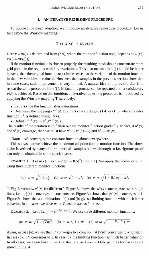
EXAMPLE 1. Let u(x)= exp(−20(x − 0.5)2) on [0, 1]. We apply the above iterationusing three different monitor functions:

(a) w =√

1+ u2x, (b) w =

√1+ u2, (c) w =

√1+ 0.1u2

x + u2.

In Fig. 3, we showuk(x) for differentk. Figure 3a shows thatuk(x) converges to two straightlines, i.e.,|uk

x(x)| converges to constants a.e. Figure 3b shows that|uk(x)| converges to 1.Figure 3c shows that a combination of (a) and (b) gives a limiting function with much betterbehavior. In all cases, we havew→ Constant a.e. ask→∞.

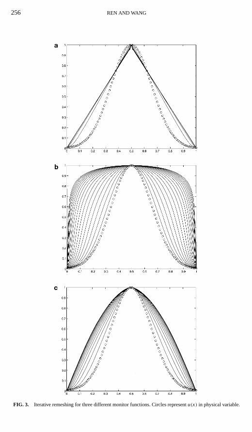
EXAMPLE 2. Letu(x, y)= e(−5(x2+y2)). We use three different monitor functions:

(a) w =√

1+ |∇u|2, (b) w =√

1+ u2, (c) w =√

1+ |∇u|2+ u2.

Again, in case (a), we see thatuk converges to a cone so that|∇u|2 converges to a constant.In case (b),|uk| converges to 1. In case (c), the limiting function has much better behavior.In all cases, we again havew → Constant a.e. ask→∞. Only pictures for case (a) areshown in Fig. 4.

256 REN AND WANG

FIG. 3. Iterative remeshing for three different monitor functions. Circles representu(x) in physical variable.

ITERATIVE GRID REDISTRIBUTION 257

FIG. 4. Iterative remeshing in two dimensions with monitor functionw=√

1+ |∇u|2.

The above examples also suggest that to achieve better limiting behavior in the compu-tational domain, the monitor function should include both|u| and|∇u|. Theoretically, themore higher order derivatives are added (although difficult to implement in practice), thebetter limiting behavior of the function in the computational domain is expected. To seethis, let the monitor function bew=

√1+ |u| + |Du| + |D2u|. Since in the iteration limit,

the monitor functionw tends to a constant, which is the integral average ofw, we have that,in the computational variables, max|Du|, max|D2u| are all bounded by the same constant.

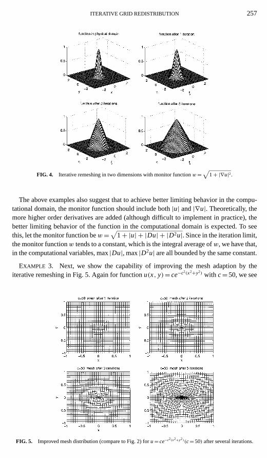
EXAMPLE 3. Next, we show the capability of improving the mesh adaption by theiterative remeshing in Fig. 5. Again for functionu(x, y)= ce−c2(x2+y2) with c= 50, we see

FIG. 5. Improved mesh distribution (compare to Fig. 2) foru= ce−c2(x2+y2)(c= 50) after several iterations.

258 REN AND WANG

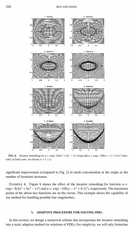
FIG. 6. Iterative remeshing foru= exp(−8(4x2+ 9y2− 1)2) (top) andu= exp(−100(y− x2+ 0.5)2) (bot-tom). In both cases, we choosew= 1+ u.

significant improvement (compared to Fig. 2) in mesh concentration at the origin as thenumber of iterations increases.

EXAMPLE 4. Figure 6 shows the effect of the iterative remeshing for functionu=exp(−8(4x2+9y2−1)2) andu= exp(−100(y− x2+0.5)2), respectively. The maximumpoints of the above two functions are on the curves. This example shows the capability ofour method for handling possible line singularities.

5. ADAPTIVE PROCEDURE FOR SOLVING PDE S

In this section, we design a numerical scheme that incorporates the iterative remeshinginto a static adaptive method for solutions of PDEs. For simplicity, we will only formulate

ITERATIVE GRID REDISTRIBUTION 259

the scheme in two dimensions. Generalization to three dimensions is straightforward. Ourscheme is static; i.e., we use a fixed grid to solve the PDE in the computational variablesuntil a certain criterion is violated that indicates that the adaption is needed. Then iterativeremeshing is used to generate a new grid.

Let’s assume that we solve a PDE or system of PDEs of the form

ut = F(x, u, Du, D2u), x ∈ Äp, (5.1)

supplemented with initial and boundary conditions.D is the first-order differential operator.The one level grid generation is based on (2.9),{∇ · ( 1

w∇ξ) = 0

∇ · ( 1w∇η) = 0,

(5.2)

which determines the transformation(x(ξ, η), y(ξ, η)) from the computational domainÄc

to the physical domainÄp. The choice of the monitor functionw is problem dependent. Inmost cases,w=

√1+ α|∇ Eu|2+ β|Eu|2 is good enough for certain constantsα > 0, β > 0.

The procedure is described in the following:

(0) Given an initial conditionEu(x, y, 0), the initial grid transformsx(ξ, η), y(ξ, η) aredetermined from the iterative remeshing, which in turn gives an initial condition in thecomputational domainEu(x(ξ, η), y(ξ, η),0).

(1) Solve the PDE in the computational variablesξ, η with the grid transformationx(ξ, η), y(ξ, η) being fixed, until some timet∗ when the solutionEu(ξ, η, t∗) cannot meet acertain criterion.

(2) Generate a new mesh by the iterative remeshing, starting withEu(ξ, η, t∗). The remesh-ing iteration stops if the criterion in (1) is satisfied. The interpolation is used to move thesolution on the new grids.

(3) Go to (1) to continue the integration.

Remark 1. The stopping criterion in step (1) depends on the specific problem. In ournumerical examples below, the criterion is set so that the maximum amplitude of the gradientis smaller than a given value TOL. The choice of TOL is flexible. However, it has to belarger than the integral average of the gradient of the solution over the domain. It is easyto see that a smaller TOL requires more remeshing iterations. In actual applications, oneshould include quantities of interests near the singularity in both the monitor function andthe stopping criterion. For example, in the fluid problem, vorticity might be the desiredquantity to be included in the monitor function.

Remark 2. In most of the cases, only one remeshing iteration is needed when we startthe iteration withEu(ξ, η, t∗) in Step 2. Since we always start the iteration from the mostrecent solution in the computational domain, when the cycle (1)–(3) is repeatedk times,effectively we have at leastk remeshing iterations att∗ from the solution in the originalphysical variables.

Remark 3. Our grid movement method is static; i.e., the grids are held stationary duringthe evolution of PDEs until the stopping criterion is violated and are shifted to their new po-sitions by our iterative procedure. The solution values are moved from the old grid to the newgrid by interpolation. The interpolation is carried out on the uniform mesh and using cubicpolynomial interpolations. As pointed out in Remark 2, our iterative procedure was carried

260 REN AND WANG

out gradually as the solution evolves toward the singularity and solution behavior in the com-putational domain is always controlled by the stopping criterion (e.g., max|∇u| ≤ TOL).Therefore interpolation errors are also controlled.

6. NUMERICAL EXAMPLES

We first solve the nonlinear Schr¨odinger equation (NLS),{iψt +1ψ + |ψ |2σψ = 0, (x, y) ∈ Äp, t > 0,

ψ(x, y, t)|∂Äp = 0,(6.1)

in two dimensions. The singular solutions with one blowup point were successfully com-puted using the dynamic rescaling method first developed in [12] for the radially symmetriccase and generalized in two and three dimensions in [11]. We shall first reproduce the resultfor the single blowup point. Then we will present an example with multiple blowup pointsas well as an example in the supercritical case.

Let (x(ξ, η), y(ξ, η)) be the spatial coordinate transformations. BothÄp (the physicaldomain) andÄc (the computational domain) are chosen to be [−1, 1]× [−1, 1]. As in thedynamic rescaling, we also rescale the time fromt to τ as

dτ

dt= 1

λ2(t). (6.2)

Let

ψ = 1

L(t)φ,

whereL(t) is a scaling factor chosen to be

L(t) = 1

max(x,y)∈Äp |ψ(x, y, t)| . (6.3)

To balance the coefficients in the transformed equation, we chooseλ= Lσ . In the coordinatesystem(ξ, η, τ ), the NLS becomes

φτ − LτLφ − i

(λ21Bφ + |φ|2φ

) = 0, (6.4)

together with

Lτ = L2σ+1 Im(φ∗1Bφ)|(ξ0,η0), (6.5)

where(ξ0(t), η0(t)) is the maximum point of|φ(ξ, η, t)|, and

1Bφ = 1

J

{∂

∂ξ

(b22φξ − b12φη

J

)+ ∂

∂η

(b11φη − b12φξ

J

)},

b11 = x2ξ + y2

ξ , b12 = xξ xη + yξ yη, b22 = x2η + y2

η .

J is the Jacobian of the coordinate transformation.In the grid redistribution, the monitor function is taken to bew(ξ, η)= (1+2|φ(ξ, η)|2+|∇φ(ξ, η)|2) . The criterion is set so that the maximum amplitude of the gradient is smallerthan a given value of TOL. Two values of TOL, 5 and 7, are used for our computations.

ITERATIVE GRID REDISTRIBUTION 261

FIG. 7. φ(ξ, η, τ ) inÄc (computational domain) atτ = 95.82(t = 0.024317104), 1/λ= 2.9514e+ 05 (NLSwith initial value (i)).

1. In the first example, we solve the NLS in the critical case (σ = 1) with the initialcondition

i. ψ(x, y, 0) = 10e−4x2−9y2.

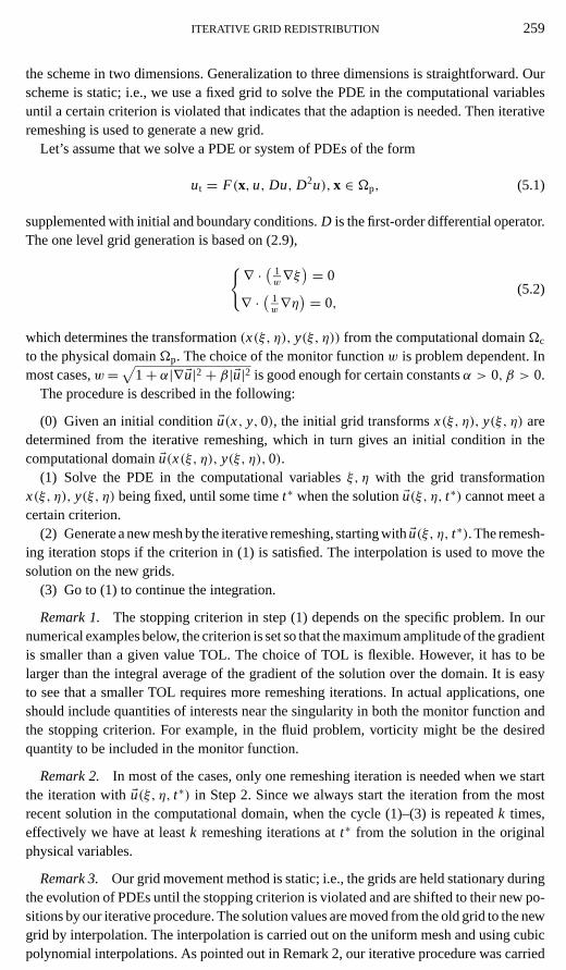
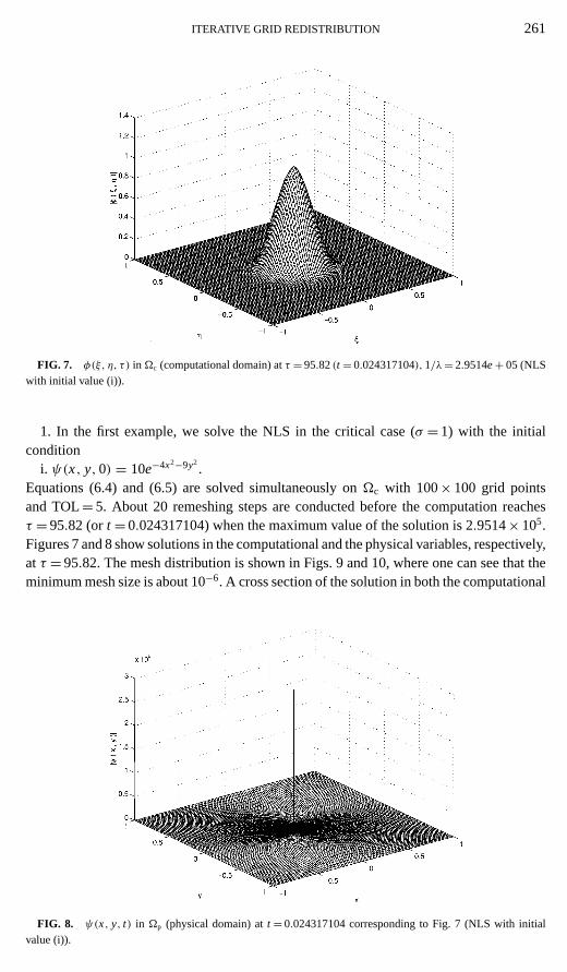
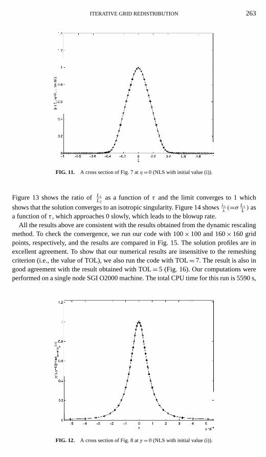
Equations (6.4) and (6.5) are solved simultaneously onÄc with 100× 100 grid pointsand TOL= 5. About 20 remeshing steps are conducted before the computation reachesτ = 95.82 (ort = 0.024317104) when the maximum value of the solution is 2.9514× 105.Figures 7 and 8 show solutions in the computational and the physical variables, respectively,at τ = 95.82. The mesh distribution is shown in Figs. 9 and 10, where one can see that theminimum mesh size is about 10−6. A cross section of the solution in both the computational

FIG. 8. ψ(x, y, t) in Äp (physical domain) att = 0.024317104 corresponding to Fig. 7 (NLS with initialvalue (i)).

262 REN AND WANG

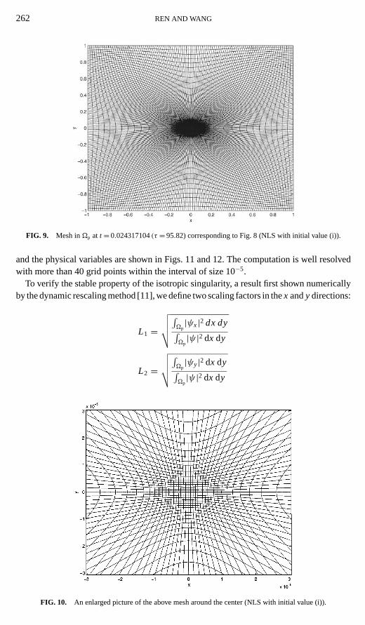
FIG. 9. Mesh inÄp at t = 0.024317104(τ = 95.82) corresponding to Fig. 8 (NLS with initial value (i)).

and the physical variables are shown in Figs. 11 and 12. The computation is well resolvedwith more than 40 grid points within the interval of size 10−5.

To verify the stable property of the isotropic singularity, a result first shown numericallyby the dynamic rescaling method [11], we define two scaling factors in thex andy directions:

L1 =√√√√∫Äp

|ψx|2 dx dy∫Äp|ψ |2 dx dy

L2 =√√√√∫Äp

|ψy|2 dx dy∫Äp|ψ |2 dx dy

FIG. 10. An enlarged picture of the above mesh around the center (NLS with initial value (i)).

ITERATIVE GRID REDISTRIBUTION 263

FIG. 11. A cross section of Fig. 7 atη= 0 (NLS with initial value (i)).

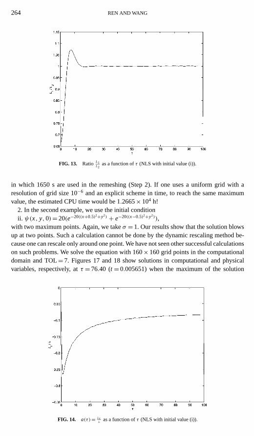
Figure 13 shows the ratio ofL1L2

as a function ofτ and the limit converges to 1 which

shows that the solution converges to an isotropic singularity. Figure 14 showsλτλ(=σ Lτ

L ) asa function ofτ , which approaches 0 slowly, which leads to the blowup rate.

All the results above are consistent with the results obtained from the dynamic rescalingmethod. To check the convergence, we run our code with 100× 100 and 160× 160 gridpoints, respectively, and the results are compared in Fig. 15. The solution profiles are inexcellent agreement. To show that our numerical results are insensitive to the remeshingcriterion (i.e., the value of TOL), we also run the code with TOL= 7. The result is also ingood agreement with the result obtained with TOL= 5 (Fig. 16). Our computations wereperformed on a single node SGI O2000 machine. The total CPU time for this run is 5590 s,

FIG. 12. A cross section of Fig. 8 aty= 0 (NLS with initial value (i)).

264 REN AND WANG

FIG. 13. Ratio L1L2

as a function ofτ (NLS with initial value (i)).

in which 1650 s are used in the remeshing (Step 2). If one uses a uniform grid with aresolution of grid size 10−6 and an explicit scheme in time, to reach the same maximumvalue, the estimated CPU time would be 1.2665× 104 h!

2. In the second example, we use the initial conditionii. ψ(x, y, 0)= 20(e−20((x+0.5)2+y2) + e−20((x−0.5)2+y2)),

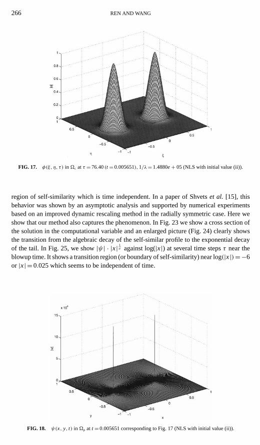
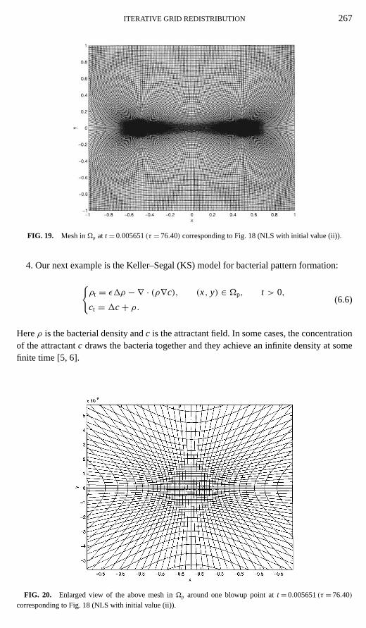
with two maximum points. Again, we takeσ = 1. Our results show that the solution blowsup at two points. Such a calculation cannot be done by the dynamic rescaling method be-cause one can rescale only around one point. We have not seen other successful calculationson such problems. We solve the equation with 160× 160 grid points in the computationaldomain and TOL= 7. Figures 17 and 18 show solutions in computational and physicalvariables, respectively, atτ = 76.40 (t = 0.005651) when the maximum of the solution

FIG. 14. a(τ )= λτλ

as a function ofτ (NLS with initial value (i)).

ITERATIVE GRID REDISTRIBUTION 265

FIG. 15. A cross section of|ψ(x, y, t)| at y= 0, τ = 95.82. 100× 100(160× 160) grid points are used for∗(—), and the maximum value at this time is 2.9514e+ 05(2.7568e+ 05). TOL= 5 (NLS with initial value (i)).

reaches 1.488× 105. The grid distribution at the same time is shown in Figs. 19 and 20. Theblowup structure of each singularity is the same as that of the solution with single blowuppoint.

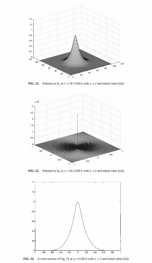
3. In the third example, we solve the NLS in the supercritical case (σ = 2) with initialcondition

iii. ψ(x, y, 0)= 10e−9x2−9y2.

The dynamics is much faster in the rescaled time variableτ than in the critical case. We plotthe solution atτ = 34.3 in both computational variables and physical variables in Figs. 21and 22. A distinct property of the supercritical collapse is that there seems to be a finite

FIG. 16. A cross section of|ψ(x, y, t)| at y= 0, τ = 95.82. TOL= 7(TOL= 5) is used for∗ (—), and themaximum value at this time is 2.9279e+ 05(2.7568e+ 05). 160× 160 (NLS with initial value (i)).

266 REN AND WANG

FIG. 17. φ(ξ, η, τ ) in Äc at τ = 76.40(t = 0.005651), 1/λ= 1.4880e+ 05 (NLS with initial value (ii)).

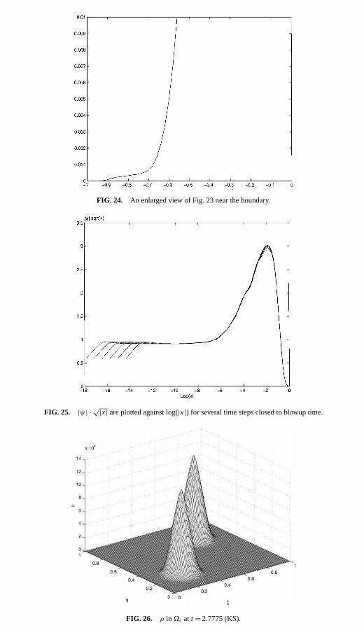
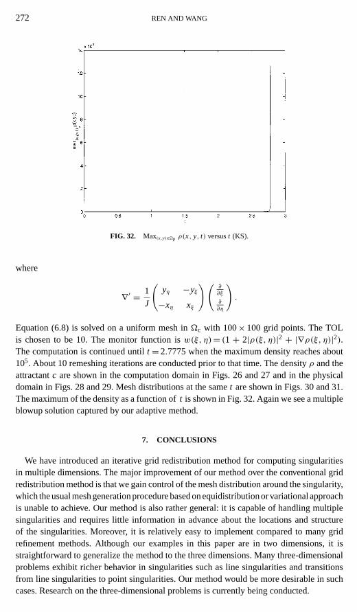
region of self-similarity which is time independent. In a paper of Shvetset al. [15], thisbehavior was shown by an asymptotic analysis and supported by numerical experimentsbased on an improved dynamic rescaling method in the radially symmetric case. Here weshow that our method also captures the phenomenon. In Fig. 23 we show a cross section ofthe solution in the computational variable and an enlarged picture (Fig. 24) clearly showsthe transition from the algebraic decay of the self-similar profile to the exponential decayof the tail. In Fig. 25, we show|ψ | · |x| 1σ against log(|x|) at several time stepsτ near theblowup time. It shows a transition region (or boundary of self-similarity) near log(|x|)=−6or |x| =0.025 which seems to be independent of time.

FIG. 18. ψ(x, y, t) in Äp at t = 0.005651 corresponding to Fig. 17 (NLS with initial value (ii)).

ITERATIVE GRID REDISTRIBUTION 267

FIG. 19. Mesh inÄp at t = 0.005651(τ = 76.40) corresponding to Fig. 18 (NLS with initial value (ii)).

4. Our next example is the Keller–Segal (KS) model for bacterial pattern formation:

{ρt = ε1ρ −∇ · (ρ∇c), (x, y) ∈ Äp, t > 0,

ct = 1c+ ρ. (6.6)

Hereρ is the bacterial density andc is the attractant field. In some cases, the concentrationof the attractantc draws the bacteria together and they achieve an infinite density at somefinite time [5, 6].

FIG. 20. Enlarged view of the above mesh inÄp around one blowup point att = 0.005651(τ = 76.40)corresponding to Fig. 18 (NLS with initial value (ii)).

FIG. 21. Solution inÄc at τ = 34.3 (NLS withσ = 2 and initial value (iii)).

FIG. 22. Solution inÄp at τ = 34.3 (NLS withσ = 2 and initial value (iii)).

FIG. 23. A cross section of Fig. 21 atη= 0 (NLS withσ = 2 and initial value (iii)).

268

FIG. 24. An enlarged view of Fig. 23 near the boundary.

FIG. 25. |ψ | · √|x| are plotted against log(|x|) for several time steps closed to blowup time.

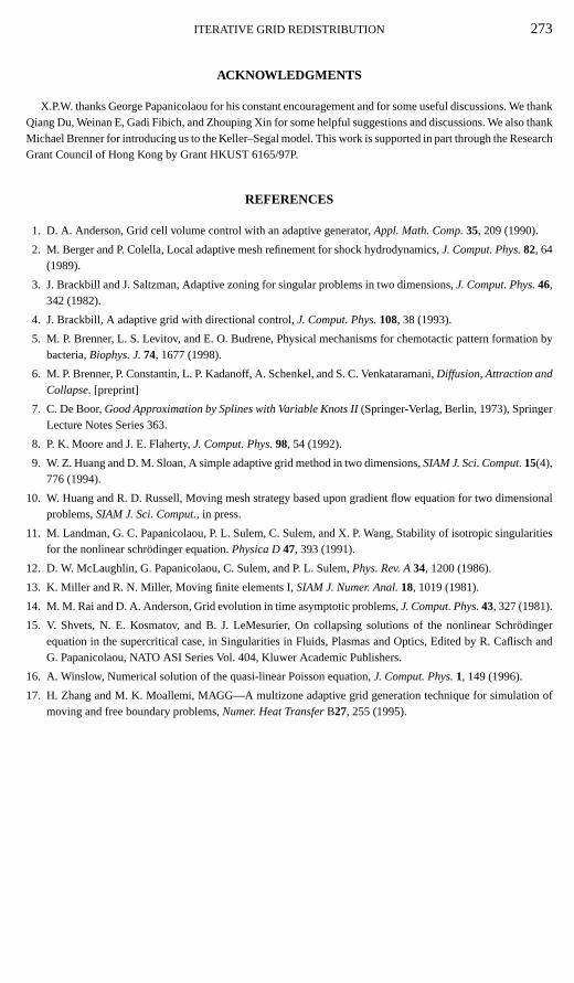
FIG. 26. ρ in Äc at t = 2.7775 (KS).

269

FIG. 27. c in Äc at t = 2.7775 (KS).

FIG. 28. ρ in Äp at t = 2.7775 corresponding to Fig. 26 (KS).

FIG. 29. c in Äp at t = 2.7775 corresponding to Fig. 27 (KS).

270

ITERATIVE GRID REDISTRIBUTION 271

FIG. 30. Mesh inÄp at t = 2.7775 corresponding to Figs. 28 and 29 (KS).

We start with a uniform density distribution and a perturbation in the attractant field ona periodic domain [0, 1]× [0, 1]:{

ρ(x, y, 0) = 1,

c(x, y, 0) = sin 2πx sin 2πy.(6.7)

Theε is taken to be 0.01. On the computational domain, the PDEs have the form of{ρt = ε1Bρ − ρ1Bc−∇′ρ · ∇′c,ct = 1Bc+ ρ, (6.8)

FIG. 31. Mesh inÄp around one blowup point att = 2.7775 corresponding to Figs. 28 and 29 (KS).

272 REN AND WANG

FIG. 32. Max(x,y)∈Äp ρ(x, y, t) versust (KS).

where

∇′ = 1

J

(yη −yξ

−xη xξ

)(∂∂ξ

∂∂η

).

Equation (6.8) is solved on a uniform mesh inÄc with 100× 100 grid points. The TOLis chosen to be 10. The monitor function isw(ξ, η)= (1 + 2|ρ(ξ, η)|2 + |∇ρ(ξ, η)|2).The computation is continued untilt = 2.7775 when the maximum density reaches about105. About 10 remeshing iterations are conducted prior to that time. The densityρ and theattractantc are shown in the computation domain in Figs. 26 and 27 and in the physicaldomain in Figs. 28 and 29. Mesh distributions at the samet are shown in Figs. 30 and 31.The maximum of the density as a function oft is shown in Fig. 32. Again we see a multipleblowup solution captured by our adaptive method.

7. CONCLUSIONS

We have introduced an iterative grid redistribution method for computing singularitiesin multiple dimensions. The major improvement of our method over the conventional gridredistribution method is that we gain control of the mesh distribution around the singularity,which the usual mesh generation procedure based on equidistribution or variational approachis unable to achieve. Our method is also rather general: it is capable of handling multiplesingularities and requires little information in advance about the locations and structureof the singularities. Moreover, it is relatively easy to implement compared to many gridrefinement methods. Although our examples in this paper are in two dimensions, it isstraightforward to generalize the method to the three dimensions. Many three-dimensionalproblems exhibit richer behavior in singularities such as line singularities and transitionsfrom line singularities to point singularities. Our method would be more desirable in suchcases. Research on the three-dimensional problems is currently being conducted.

ITERATIVE GRID REDISTRIBUTION 273

ACKNOWLEDGMENTS

X.P.W. thanks George Papanicolaou for his constant encouragement and for some useful discussions. We thankQiang Du, Weinan E, Gadi Fibich, and Zhouping Xin for some helpful suggestions and discussions. We also thankMichael Brenner for introducing us to the Keller–Segal model. This work is supported in part through the ResearchGrant Council of Hong Kong by Grant HKUST 6165/97P.

REFERENCES

1. D. A. Anderson, Grid cell volume control with an adaptive generator,Appl. Math. Comp.35, 209 (1990).

2. M. Berger and P. Colella, Local adaptive mesh refinement for shock hydrodynamics,J. Comput. Phys.82, 64(1989).

3. J. Brackbill and J. Saltzman, Adaptive zoning for singular problems in two dimensions,J. Comput. Phys.46,342 (1982).

4. J. Brackbill, A adaptive grid with directional control,J. Comput. Phys.108, 38 (1993).

5. M. P. Brenner, L. S. Levitov, and E. O. Budrene, Physical mechanisms for chemotactic pattern formation bybacteria,Biophys. J.74, 1677 (1998).

6. M. P. Brenner, P. Constantin, L. P. Kadanoff, A. Schenkel, and S. C. Venkataramani,Diffusion, Attraction andCollapse. [preprint]

7. C. De Boor,Good Approximation by Splines with Variable Knots II(Springer-Verlag, Berlin, 1973), SpringerLecture Notes Series 363.

8. P. K. Moore and J. E. Flaherty,J. Comput. Phys.98, 54 (1992).

9. W. Z. Huang and D. M. Sloan, A simple adaptive grid method in two dimensions,SIAM J. Sci. Comput.15(4),776 (1994).

10. W. Huang and R. D. Russell, Moving mesh strategy based upon gradient flow equation for two dimensionalproblems,SIAM J. Sci. Comput., in press.

11. M. Landman, G. C. Papanicolaou, P. L. Sulem, C. Sulem, and X. P. Wang, Stability of isotropic singularitiesfor the nonlinear schr¨odinger equation.Physica D47, 393 (1991).

12. D. W. McLaughlin, G. Papanicolaou, C. Sulem, and P. L. Sulem,Phys. Rev. A34, 1200 (1986).

13. K. Miller and R. N. Miller, Moving finite elements I,SIAM J. Numer. Anal.18, 1019 (1981).

14. M. M. Rai and D. A. Anderson, Grid evolution in time asymptotic problems,J. Comput. Phys.43, 327 (1981).

15. V. Shvets, N. E. Kosmatov, and B. J. LeMesurier, On collapsing solutions of the nonlinear Schr¨odingerequation in the supercritical case, in Singularities in Fluids, Plasmas and Optics, Edited by R. Caflisch andG. Papanicolaou, NATO ASI Series Vol. 404, Kluwer Academic Publishers.

16. A. Winslow, Numerical solution of the quasi-linear Poisson equation,J. Comput. Phys.1, 149 (1996).

17. H. Zhang and M. K. Moallemi, MAGG—A multizone adaptive grid generation technique for simulation ofmoving and free boundary problems,Numer. Heat TransferB27, 255 (1995).