Iterative Methods for the Solution of a Singular Control Formulation of a GMWB Pricing Problem * Y. Huang † P.A. Forsyth ‡ G. Labahn § February 3, 2011 Abstract Discretized singular control problems in finance result in highly nonlinear algebraic equations which must be solved at each timestep. We consider a singular stochastic control problem arising in pricing a Guaranteed Minimum Withdrawal Benefit (GMWB), where the underlying asset is assumed to follow a jump diffusion process. We use a scaled direct control formulation of the singular control problem and examine the conditions required to ensure that a fast fixed point policy iteration scheme converges. Our methods take advantage of the special structure of the GMWB problem in order to obtain a rapidly convergent iteration. The direct control method has a scaling parameter which must be set by the user. We give estimates for bounds on the scaling parameter so that convergence can be expected in the presence of round-off error. Example computations verify that these estimates are of the correct order. Finally, we compare the scaled direct control formulation to a formulation based on an improved version of the penalty method. We show that the scaled direct control method has some advantages over the penalty method. Keywords: HJB equation, singular control, scaled direct control, iterative methods, jump diffusion AMS Classification 65N06, 93C20 1 Introduction Stochastic control problems arise in many financial applications, often in one of two forms: impulse control [6] and singular control [22, 18, 9]. The main computational cost of solution of an impulse control problem is the search for a global minimum along trajectories emanating from each node [6]. In contrast, discretization of singular control formulations requires the solution of a system of nonlinear algebraic equations at each timestep, which is a significant computational hurdle. In * This work was supported by Credit Suisse, New York and the Natural Sciences and Engineering Research Council of Canada † Department of Electrical and Computer Engineering, University of Waterloo, Waterloo ON, Canada N2L 3G1, [email protected]‡ Cheriton School of Computer Science, University of Waterloo, Waterloo ON, Canada N2L 3G1 [email protected]§ Cheriton School of Computer Science, University of Waterloo, Waterloo ON, Canada N2L 3G1 [email protected]1
Transcript
Iterative Methods for the Solution of a Singular Control
Formulation of a GMWB Pricing Problem ∗
Y. Huang † P.A. Forsyth ‡ G. Labahn §
February 3, 2011
Abstract
Discretized singular control problems in finance result in highly nonlinear algebraic equationswhich must be solved at each timestep. We consider a singular stochastic control problem arisingin pricing a Guaranteed Minimum Withdrawal Benefit (GMWB), where the underlying assetis assumed to follow a jump diffusion process. We use a scaled direct control formulation ofthe singular control problem and examine the conditions required to ensure that a fast fixedpoint policy iteration scheme converges. Our methods take advantage of the special structureof the GMWB problem in order to obtain a rapidly convergent iteration. The direct controlmethod has a scaling parameter which must be set by the user. We give estimates for boundson the scaling parameter so that convergence can be expected in the presence of round-off error.Example computations verify that these estimates are of the correct order. Finally, we comparethe scaled direct control formulation to a formulation based on an improved version of thepenalty method. We show that the scaled direct control method has some advantages over thepenalty method.
Stochastic control problems arise in many financial applications, often in one of two forms: impulsecontrol [6] and singular control [22, 18, 9]. The main computational cost of solution of an impulsecontrol problem is the search for a global minimum along trajectories emanating from each node[6]. In contrast, discretization of singular control formulations requires the solution of a systemof nonlinear algebraic equations at each timestep, which is a significant computational hurdle. In
∗This work was supported by Credit Suisse, New York and the Natural Sciences and Engineering Research Councilof Canada†Department of Electrical and Computer Engineering, University of Waterloo, Waterloo ON, Canada N2L 3G1,
[email protected]‡Cheriton School of Computer Science, University of Waterloo, Waterloo ON, Canada N2L 3G1
[email protected]§Cheriton School of Computer Science, University of Waterloo, Waterloo ON, Canada N2L 3G1
this article, we consider the singular control formulation of a particular financial contract, theGuaranteed Minimum Withdrawal Benefit (GMWB) contract [17, 9, 13] and provide an efficientmethod for numerically pricing such a contract. Although we focus specifically on GMWB problemshere, our results and methods of analysis are applicable to many other singular control problemsin finance.
It is worthwhile to note that there are several approaches for solution of singular stochasticcontrol problems. Markov chain methods [16, 12, 5] are essentially explicit finite difference schemes,and hence suffer from the usual timestep limitations due to stability considerations. Anotherapproach is based on front tracking, whereby the boundaries between different regions (in ourcase the finite and infinite withdrawal domains) are tracked, usually by enforcing some some typeof smooth pasting condition [15]. This method becomes complex if the different regions becomemultiply connected. We restrict attention in the following to methods which are unconditionallystable, and do not require explicit tracking of internal boundaries.
The GMWB pricing problem requires the solution of a Hamilton Jacobi Bellman (HJB) Varia-tional Inequality (VI). It is necessary to discretize this HJB VI so that convergence to the viscositysolution is ensured [2, 1]. Generally, the viscosity solution of the HJB VI can be shown to be thesolution of the contract valuation problem posed as a dynamic program, which is the financiallyrelevant solution. In [9, 13], a penalty method is used to discretize the HJB VI arising from aGMWB contract. This method is shown to be monotone, consistent and l∞ stable [13], and henceconvergence to the viscosity solution is ensured assuming a strong comparison property holds.The authors in [13] use a fully implicit timestepping method which guarantees an unconditionallymonotone discretization. The method gives rise to a nonlinear system of algebraic equations ateach timestep.
In this paper we use a scaled direct control method for solving the singular control formulationof the GMWB problem. The direct control technique was previously suggested for solving Americanoption type problems [14, 4]. In addition, we consider the case where the underlying risky assetfollows a jump diffusion process [8]. The method makes use of a fully implicit discretization whichis shown to be monotone, consistent and l∞ stable. We introduce a scaling factor in our directcontrol formulation, which allows us to solve the associated nonlinear algebraic equations using thefixed-point policy iteration method of [14].
Our discretization of the singular control GMWB problem has a special structure that alsoallows for rapid solution of the associated nonlinear algebraic equations. We present a block matrixfixed-point policy iteration scheme for solving the nonlinear algebraic equations and show that ithas the same convergence properties as fixed-point policy iteration. Numerical experiments implythat the number of iterations required for convergence of the block method is an order of magnitudeless than required for the full matrix version. In an Appendix we also present a block matrix fixed-point policy iteration scheme for the algebraic equations that arise from the discretization of thepenalty method. This allows us to properly compare the scaled direct control and penalty methodson an equal footing.
The direct control technique (and also the penalty method) require the specification of a pa-rameter which may affect solution accuracy and convergence of the iteration. We carry out ananalysis of this parameter (for both formulations). We estimate bounds for the scaling factor (di-rect control) and the penalty factor (penalty method) so that convergence can be expected in thepresence of roundoff error. Numerical experiments verify that these bounds are of the correct orderof magnitude. Both the analysis and the experimental results indicate that the useful numerical
2
range of the scaling parameter (direct control) is much larger than for the penalty factor (penaltymethod).
The block matrix fixed-point policy iteration for the GMWB problem also has the advantageof being relatively simple to implement. Indeed the primary tools needed are a tridiagonal matrixsolver and a procedure for finding maxima of finite sets of values.
The remainder of the paper is organized as follows. The following section gives the details of aGMWB contract and its formulation as a singular stochastic control problem. Section 3 gives thediscretization of the scaled direct control form of the HJB VI and describes the nonlinear algebraicequations that need to be solved at every timestep. In Section 4 we show that the fixed-point policyiteration algorithm of [14] can be used to solve the nonlinear equations in full matrix form. Section5 describes a block matrix fixed-point policy iteration method and gives the details for verifyingthe necessary convergence properties. Section 6 considers the case where floating point arithmeticimpacts the mathematical results. Numerical tests are presented in the following section. Thepaper ends with a conclusion and an Appendix, with the Appendix giving details of the blockmatrix fixed point method as applied to the penalty method, the discretization details and finallysome floating point error analysis needed in the main text.
2 Singular Control Formulation of the GMWB Problem
2.1 Motivation
Many holders of a defined contribution pension plan are responsible for investing a portfolio ofassets which generate cash flows during their retirement. A GMWB contract consists of an initiallump sum payment to an insurance companys which is then invested in risky assets. The holder isallowed to withdraw a specified amount each year of the contract, regardless of the performance ofthe risky asset, with withdrawals above the contract rate being subject to a penalty. At the endof the contract, the holder receives any investment amount remaining. Thus the holder of such acontract receives a minimum guaranteed yearly income, but can also participate in market gains.In return for providing this guarantee, the insurance company charges a proportional fee, which isextracted from the risky investment portfolio. The pricing problem is to determine the proportionalfee that needs to be charged.
2.2 Formulation
Dai et al [9] formulated the GMWB pricing problem using a singular stochastic control formula-tion under the assumption that the underlying risky asset follows a constant volatility geometricBrownian motion process. In this section we review an extension to the Dai formulation given inHuang et al [13] where the risky asset is assumed to follow a jump diffusion process. The dynamicsof the underlying asset W is given by the following stochastic differential equation
dW = (r − η − λρ)Wdt+ σWdZ + (ξ − 1)Wdq + dA, if W > 0 (2.1)
dW = 0, if W = 0, (2.2)
where dZ is the increment of a Weiner process and A is the investor’s virtual guarantee withdrawalaccount. In the above, r is the risk free rate, σ is the volatility and η the fee charged for the
3
guarantee. The variable λ is the jump intensity representing the mean arrival rate of the Poissonprocess:
dq =
0 with probability 1− λdt1 with probability λdt
, (2.3)
with ξ a random variable representing the jump size of W . We assume that ξ follows a log-normaldistribution p(ξ) given by
p(ξ) =1√
2πζξexp(−(log(ξ)− ν)2
2ζ2
), (2.4)
with parameters ζ and ν, ρ = E[ξ − 1], where E[·] is the expectation, and E[ξ] = exp(ν + ζ2/2)given the distribution function p(ξ) in (2.4).
The second variable in a GMWB contract is the investor’s virtual guarantee account A. Thewithdrawal feature is modeled with parameters G, the contractual withdrawal rate and κ < 1, theproportional penalty charge. Define τ = T − t where t is the forward time, and T is the expiry timeof the contract and set V = V (W,A, τ) to be the no arbitrage value of the guarantee. Generalizingthe formulation in [17, 9, 14] to the case with a stochastic jump process (2.1), the value of theguarantee is given from the solution to the following singular control problem
min
[Vτ − LV − λJ V −Gmax(FV, 0) , κ−FV
]= 0 . (2.5)
Here the operators L,F ,J are defined as
LV =σ2
2W 2VWW + (r − η − λρ)WVW − (r + λ)V
=σ2
2W 2DWWV + (r − η − λρ)WDWV − (r + λ)V
FV = 1− VW − VA = 1−DWV −DAV
J V =
∫ ∞0
V (ξW,A, τ)p(ξ) dξ , (2.6)
while DA, DW , and DWW denote the usual partial derivative operators.
2.3 The Scaled Direct Control form of the Pricing Problem
The control form of equation (2.5) is given by
minϕ∈0,1,ψ∈0,1
ϕψ=0
[ψ(κ−FV ) + (1− ψ)(Vτ − LV − λJ V − ϕGFV )
]= 0 . (2.7)
Observe that that the term κ−FV is dimensionless whereas Vτ−LV −Gmax(FV, 0) has dimensionsof currency/time. Hence equation (2.7) compares quantities having different units. Of course, inexact arithmetic, this is not an issue of importance. However, an iterative procedure for solution ofthe discretized equations will involve a test comparing two (in general) non-zero quantities. Hencescaling becomes important. Consequently, we introduce a scaling factor Π > 0 into equation (2.7)
minϕ∈0,1,ψ∈0,1
ϕψ=0
[Πψ(κ−FV ) + (1− ψ)(Vτ − LV − λJ V − ϕGFV )
]= 0 . (2.8)
4
Remark 2.1 (Scaling Factor). By introducing a scaling factor with dimension of currency/time,we ensure the comparison in equation (2.8) is conducted on two items with the same units. Ofcourse, this still leaves the size of the scaling factor as arbitrary. We will exploit this fact to ensurethat convergence of our iterative method can be guaranteed with a suitable choice for Π.
Problem (2.5), or equivalently, (2.8) is solved on the computational domain
(W,A, τ) ∈ [0,Wmax)× [0, ω0]× [0, T ] , (2.9)
where ω0 denotes the initial premium. At expiry time τ = 0, the value of the contract is
V (W,A, τ = 0) = max
[W, (1− κ)A
]. (2.10)
Other boundary conditions are
min
[Vτ − rV −Gmax(1− VA, 0), κ− (1− VA)
]= 0 ; W = 0 ,
V (Wmax, A, τ) = e−ητWmax ; W = Wmax ,
VWW → 0 ; W →Wmax ,
Vτ = LV − λJ V ; A = 0 . (2.11)
The boundary condition at W = 0 is a variational inequality which normally can also be solvedas a control equation. No boundary condition is required at A = ω0. For details concerningthe derivation of equation (2.5), we refer readers to [17, 6, 7, 9, 13]. The condition VWW → 0,W → Wmax assumes linear behaviour of the solution for W → Wmax. This condition was usedin [10, 24] so that the combined jump terms vanish, which eliminates the necessity of estimatingvalues outside the computational domain.
2.4 No-arbitrage Fee
Since no fee is paid up-front, the insurance company needs to charge a proportional fee η (seeequation (2.1)), such that the value of the contract is equal to the initial premium. If ω0 denotesthis initial premium and V (η;W,A, τ) is the value of the contract as a function of η, then theno-arbitrage fee is the solution to the equation
V (η;ω0, ω0, T ) = ω0 . (2.12)
3 GMWB: Discretization
In order to solve equation (2.8), we discretize each equation over a finite grid in the W×A plane. De-fine a set of nodes in the W direction W1,W2, ...,Wimax and in the A direction A1, A2, ..., Ajmax.Denote the nth timestep by τn = n∆τ and let V n
i,j be the approximate solution of equation (2.8)at (Wi, Aj , τ
n). We discretize equation (2.8) using fully implicit timestepping and central, forwardand backward differencing so that the positive coefficient condition is satisfied [11, 13, 25]. Forefficiency, central differencing is used as much as possible [25].
Let Lh,Fh,DhW ,DhA (defined in Appendix B.1 and B.2) be the discrete forms of the operatorsL,F ,DW ,DA, respectively and let J h be the discretized J operator. The integral term J V is
5
discretized via transformation into a correlation integral combined with a use of the midpoint ruleas described in detail in [10, 24].
Equation (2.8) is then written in the discrete form
(1− ψi,j)(
1
∆τV n+1i,j − LhV n+1
i,j + ϕi,jG(DhWV n+1i,j +DhAV n+1
i,j )
)+ Π ψi,j(DhWV n+1
i,j +DhAV n+1i,j )
= (1− ψi,j)1
∆τV ni,j + Π ψi,j(1− κ) + (1− ψi,j)
(λ[J hV n+1]i,j + ϕi,jG
)(3.1)
where
ϕi,j , ψi,j ∈ arg maxϕ∈0,1,ψ∈0,1
ϕψ=0
Π ψ(κ−FhV n+1
i,j )− (1− ψ)
(V n+1i,j − V n
i,j
∆τ
−(LhV n+1
i,j + λ[J hV n+1]i,j + ϕGFhV n+1i,j
)). (3.2)
We can also rewrite equation (3.1) in an equivalent form (replacing DhA by a backward difference)
(1− ψi,j)(
1
∆τV n+1i,j − LhV n+1
i,j + ϕi,jG(V n+1i,j
∆A−j+DhWV n+1
i,j )
)+ Π ψi,j(
V n+1i,j
∆A−j+DhWV n+1
i,j )
= (1− ψi,j)1
∆τV ni,j + Π ψi,j(1− κ+
V n+1i,j−1
∆A−j)
+(1− ψi,j)(λ[J hV n+1]i,j + ϕi,jG(
V n+1i,j−1
∆A−j+ 1)
)(3.3)
where ∆A−j = Aj −Aj−1.The boundary conditions at W = Wmax translate into the discrete equations
Vimax,j = e−ητnWmax, (3.4)
which we approximate by
(1
∆τ+ η)V n+1
imax,j=
1
∆τV nimax,j ; V 0
imax,j = Wmax . (3.5)
At W = 0, equation (3.1) holds with DhW ≡ 0. At A = 0, equation (3.1) holds with ϕi,j = 0,ψi,j = 0.
Remark 3.1. Using the methods as in [13] it is straightforward to show that scheme (3.1) ismonotone, consistent and l∞ stable.
3.1 Matrix Form of the Discretized Equations
Equations (3.1-3.3) are discretized using fully implicit method timestepping. The resulting set ofdiscrete algebraic equations then needs to be solved. We do this via a modified version of policyiteration.
6
Let N = imax × jmax be the size of the W ×A plane grid and set
` = i+ (j − 1)imax with 1 ≤ i ≤ imax and 1 ≤ j ≤ jmax, (3.8)
so that
[v∗,j ]i = vi,j
= v` with ` = i+ (j − 1)imax . (3.9)
As a result, we will sometimes refer to the same entry in the N-length vector v as v` or vi,j , with thereference being clear from the context. It is also convenient to represent the algebraic equations bymatrix notation. In this paper we use boldface capital letter T to represent an N ×N matrix withentries [T]`,m = T`,m. We will also refer to the jth imax× imax subblock of T using the notation Tj.These subblocks will be defined in later sections.
At each timestep, we must solve for the unknowns V n+1i,j . We can write these equations in
nonlinear matrix form as follows. Let [v∗,j ]i = V n+1i,j . Then, as generalized in [14], the algebraic
equations at each timestep can be written as:
supq∈Q
−T(q)v + c(q)
= 0 , (3.10)
where Q is a set of controls and for y = (y1, y2, . . . , yN )′ we have
[T(qk)y]` = [Tky]` = (1− ψk` )
(1
∆τy` − Lhy` + ϕk`G(DhW y` +DhAy`)
)+ Π ψk` (DhW y` +DhAy`)− (1− ψk` )λ[J hy]`[
c(qk, V n)]`
= (1− ψk` )1
∆τV n` + Π ψk` (1− κ) . (3.11)
Due to the nature of the jump term J [10] the matrix T is dense, which makes the standardpolicy iteration algorithm inefficient. To avoid this problem, we split T into two components A−Bsuch that A is sparse, and B is dense. Here
[A(qk)y]` = [Aky]` = (1− ψk` )
(1
∆τy` − Lhy` + ϕk`G(DhW y` +DhAy`)
)+ Π ψk` (DhW y` +DhAy`)[
B(qk)y]`
=[Bky
]`
= (1− ψk` )λ[J hy]` . (3.12)
Remark 3.2. (Structure of T(q), c(q)) It is important to observe that [T(q)]`,m, [A(q)]`,m, [B(q)]`,m,[c(q)]` depend only on q`. This is typical of discretized HJB equations.
7
Assuming that Q is a finite set, or that Q is compact and T(q) is an upper semi-continuousfunction of q, then equation (3.10) is interpreted as
T(q∗)v =[A(q∗)−B(q∗)
]v = c(q∗)
with q∗` = arg maxq`∈Q
−T(q)v + c(q)
`
= arg maxq`∈Q
−[A(q)−B(q)
]v + c(q)
`
. (3.13)
Thus the problem has a potentially different control for each row of the linear system. Note thatequation (3.10) is highly nonlinear.
Splitting the sparse and dense components implies that, rather than using the traditional policyiteration to solve the nonlinear system in (3.10), a fixed point policy iteration will be used. Thishas been shown to be more efficient [14] than the standard policy iteration. In Algorithm 1, eachiteration requires a sparse solve, and a dense matrix vector multiply, Bvk. The latter can be carriedout efficiently using an FFT as shown in [10].
Algorithm 1 Fixed Point-Policy Iteration
1: vk = (v)k with v0 = Initial solution vector of size N2: for k = 0, 1, 2, . . . until converge do
3: qk` = arg maxq`∈Q
−[A(q)−B(q)
]vk + c(q)
`
4: Solve A(qk)vk+1 = B(qk)vk + C(qk)
5: if k > 0 and max`
|vk+1` − vk` |
max[scale, vk+1
`
] < tolerance then
6: break from the iteration7: end if8: end for
The factor scale in Algorithm 1 ensures that unrealistic levels of accuracy are not required forsmall values of the solution. For example, if the option is priced in dollars, a typical value wouldbe scale = 1.
4 Full Matrix Form
While splitting our full matrix into components as in (3.12) does improve the linear solution step4 in Algorithm 1, we need to ensure that the ixed point policy iteration will converge. Suffi-cient conditions for convergence of the fixed point policy iteration were determined in [14]. Theserequirements are summarized in Condition 4.1.
Condition 4.1. The matrices A(q),B(q) and vector c(q) satisfy:
(i) The matrices A(q) and A(q)−B(q) are M matrices.
(ii) The vector c(q) and matrices A, B, and ‖A−1(q)‖∞ are bounded, independent of q.
(iii) There is a constant C1 < 1 such that
‖A−1(qk)B(qk−1)‖∞ ≤ C1 and ‖A−1(qk)B(qk)‖∞ ≤ C1. (4.1)
8
Remark 4.1. We remind the reader that a matrix A is an M matrix if A is nonsingular, A hasnon-positive off-diagonals, and A−1 ≥ 0 [23].
Theorem 4.1 (Convergence of Scheme). If the matrices A(q),B(q) and vector c(q) satisfy Con-dition 4.1, then the scheme in Algorithm 1 converges to the unique solution of equation (3.13), forany initial iterate vk.
Proof. We give a brief sketch of this proof here, and refer the reader to [14] for details. The basicidea of the proof of Theorem 4.1 is to show the algorithm generates a convergence sequence byre-arranging Algorithm 1 as:
Since ‖A−1(qk)B(qk−1)‖∞ ≤ C1 < 1, the sequence vk can be shown to be convergent [14]. Iflimk→∞ v
k = v∗, then it is easily seen from equation (4.2) that v∗ is a solution of equation (3.10).Uniqueness follows from the M matrix property of (A(q)−B(q)) [19, 4, 14].
Remark 4.2. The proof of Theorem 4.1 gives some idea of what might go wrong in floating pointenvironments. Namely, in exact arithmetic, equation (4.4) is always true. However, in floatingpoint arithmetic, equation (4.4) is not always true and indeed convergence does not always hold insuch environments. We discuss this further in a later section.
4.1 Verification of Conditions 4.1
In this subsection we verify that Conditions 4.1 are satisfied for our Direct Control discretization,at least when the scaling parameter is large enough. Unfortunately, the technique used in [14] toverify these conditions does not work in this case as there are zero row sums in the matrix A.
It is useful to separate the diagonal blocks from the lower triangular part of A by
[AkDy]` = (1− ψk` )
(1
∆τy` − Lhy` + ϕk`G
(DhW y` +
y`
∆A−j
))+ Π ψk`
(DhW y` +
y`
∆A−j
)[Ak
Ly]` = −(1− ψk` )ϕk`G
(y`−imax
∆A−j
)−Πψk`
(y`−imax
∆A−j
). (4.6)
Then Ak = AkD + Ak
L for each k.
9
Proposition 4.1. Suppose a positive coefficient discretization [11] is used and the jump operatorJ h is discretized using the method in [10]. Furthermore assume there is linear behavior of thesolution for i ≥ i [10, 24]. Then discretization (3.11) satisfies
(a) B(q) ≥ 0,
(b) The `th row sum for B(qk) is
Row Sum ` ( B(q) ) ≤
(1− ψk` )λ 1 < i < i
0 i = i, ..., imax
(4.7)
(c) The `th row sum for AD(qk) is
Row Sum ` ( AD(qk)) =
(1− ψk` )
(1
∆τ + (r + λ) + ϕk`G1
∆A−j
)+ ψk`Π 1
∆A−j1 < i < i
(1− ψk` )(
1∆τ + r + ϕk`G
1∆A−j
)+ ψk`Π 1
∆A−ji = 1; i ≤ i < imax
1∆τ + η i = 1; i = imax
(4.8)
(d) The matrices A(q)−B(q) and A(q) in equation (3.11) are M matrices.
Proof. The construction of B(q) using the discretization of J V as detailed in [10] implies that∑`
[J h]µ,` ≤ 1 and [J h]µ,` ≥ 0 . (4.9)
This holds since p(ξ) in (2.6) is a probability density function. When the grid node (i, j) satisfiesi > i then the `th row of B(q) is identically zero [10, 24]. This gives (a) and (b).
In order to prove (c), we first observe that
DhWW 1 = 0 ; DhW 1 = 0 ; ; DhA1 = 0
and Lh1 =
−(r + λ) 1 < i < i
−r i = 1; i ≤ i < imax
(4.10)
The row sum of AD is [AD(qk)e]i with e = (1, ..., 1)′, and consequently (c) follows using results(4.10), for 1 < i < imax. When i = imax then from the boundary assignment of equation (3.5), therow sum is just (1/∆τ + η).
To prove (d), note that A(q) = AD(q) + AL(q) with AD(q) block diagonal and AL(q) lowertriangular. From (c), the row sums of AD(q) are strictly positive, and off-diagonals are non-positivesince a positive coefficient discretization is used. Hence AD(q) consists of diagonal blocks, each ofwhich is a strictly diagonally dominant M matrix. Since AL(q) is non-positive, a straightforwardcomputation shows that A(q) is non-singular and that A−1(q) ≥ 0. A similar argument shows thatA(q)−B(q) is also an M matrix.
The following Lemma will be useful later on.
10
Lemma 4.1. Suppose A is a strictly diagonally dominant M matrix and B ≥ 0. Then
‖A−1B‖∞ ≤ maxi
Row Sum i (B)
Row Sum i (A). (4.11)
Proof. See [14].
Lemma 4.2. Suppose the discretization for the GMWB direct control method satisfies the condi-tions required for Proposition 4.1, and in addition
Π > Amaxλ1 + (r + λ)∆τ
1 + r∆τ. (4.12)
Then the matrices A,B satisfy Condition 4.1, and hence from Theorem 4.1, Algorithm 1 converges.
Proof. We need to show that there is a constant C1 such that
‖A−1(qk)B(qp)‖∞ ≤ C1 , (4.13)
where p = k, k − 1. Consider an arbitrary vector z, and a vector y such that
A(qk)y = B(qp)z . (4.14)
Then condition (4.13) is equivalent to requiring that
max‖z‖∞ 6=0
[‖y‖∞‖z‖∞
]≤ C1 < 1 (4.15)
From equation (3.11), we can see that [Ae]` = 0; i < i, ψk` = 1, and hence we are obliged to use adifferent method from that in [14] to prove this result.
First, note that[A(qk)y
]`
= [B(qp)z ]l ; ` = i+ (j − 1) ∗ imax ; 1 < i < i (4.16)[A(qk)y
]`
= 0 ; ` = i+ (j − 1) ∗ imax ; i = 1; i ≥ i (4.17)
due to the linear behaviour assumed for i ≥ i [10]. Define a bounding grid function y
[y]` =‖z‖∞λ∆τ
1 + (r + λ)∆τ+Aj
‖z‖∞λΠ
; ` = i+ (j − 1) ∗ imax . (4.18)
Noting properties (4.10), and
DhWAj = 0 ; DhAAj = 1 , (4.19)
and substituting equation (4.18) into equation (3.11) gives[A(qk)y
]`≥ ‖z‖∞λ ; 1 < i < i (4.20)[
A(qk)y]`≥ 0 ; i = 1; i ≥ i. (4.21)
11
Subtracting equation (4.16) from equation (4.20) yields (noting properties (a) and (b) of B inProposition 4.1) [
Since A(qk) is an M matrix, we have that y ≤ y. A similar argument gives y ≥ −y. Hence
‖y‖∞ ≤‖z‖∞λ∆τ
1 + (r + λ)∆τ+Amax
‖z‖∞λΠ
. (4.25)
As we require that ‖y‖∞ < ‖z‖∞, the condition on Π then becomes
Π > Amaxλ1 + (r + λ)∆τ
1 + r∆τ. (4.26)
5 Block Matrix Form
Let v∗,j = V n+1∗,j , and let (v∗,j)
k be the kth iterate for v∗,j . From the boundary condition (2.11), wecan observe that v∗,1 can be computed without any knowledge of interior nodes in the computationaldomain. To ensure a positive coefficient discretization, the DhA term is always backward differenced,hence v∗,j depends only on v∗,j−1 for j > 1. This special structure of the system makes the iterationmore efficient when we solve v∗,j before proceeding to solve v∗,j+1. We can write the full matrixsystem in (3.11) in block form as
A1 0 · · · 00 A2(q∗,2) · · · 0...
.... . .
...0 0 · · · Ajmax(q∗,jmax)
v∗,1v∗,2...v∗,jmax
=
B1 0 · · · 00 B2(q∗,2) · · · 0...
.... . .
...0 0 · · · Bjmax(q∗,jmax)
v∗,1v∗,2...v∗,jmax
+
c∗,1(V n)c∗,2(q∗,2, v∗,1, V
n))...c∗,jmax(q∗,jmax , v∗,jmax−1, V
n))
, (5.1)
with
qi,j = arg maxqi,j∈Q
−Aj(q∗,j)v∗,j + Bj(q∗,j)v∗,j + c∗,j(q∗,j , v∗,j−1, V
n)
i
. (5.2)
12
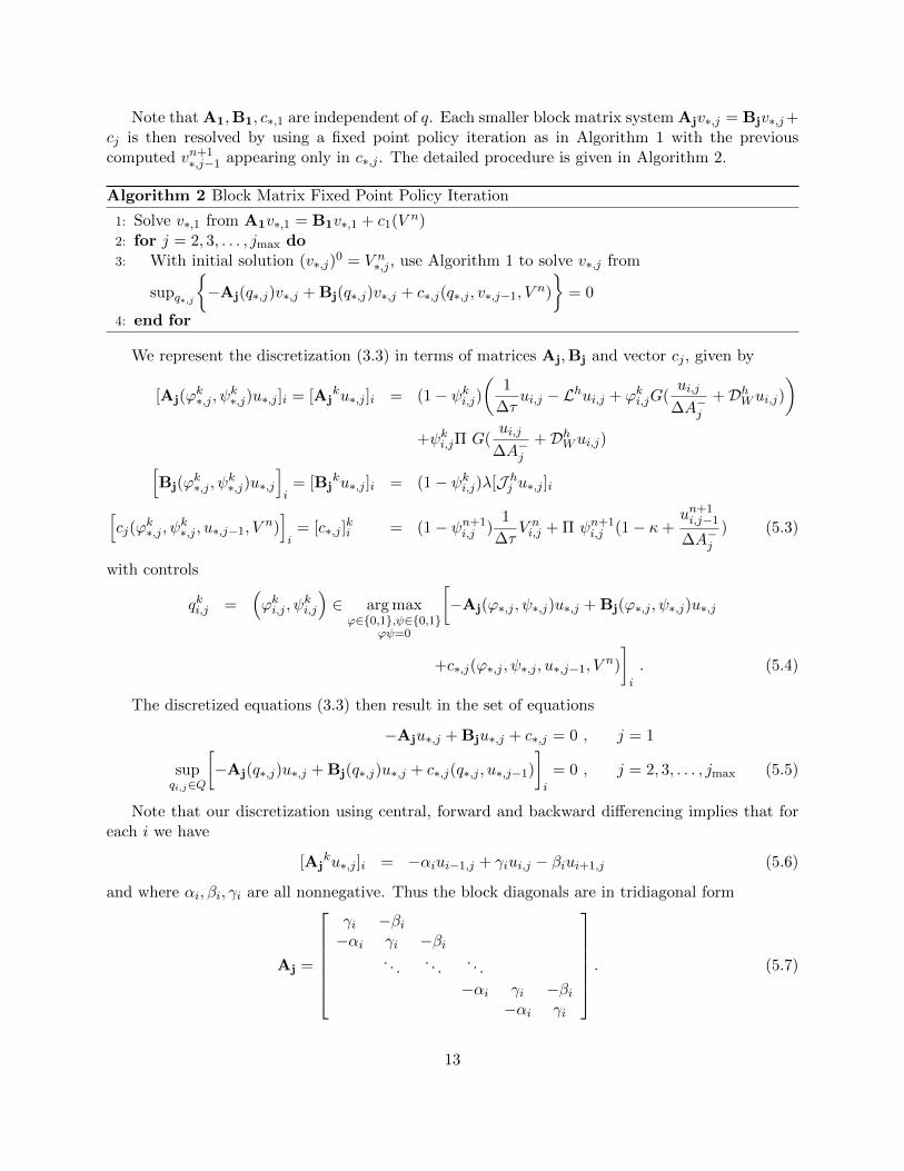
Note that A1,B1, c∗,1 are independent of q. Each smaller block matrix system Ajv∗,j = Bjv∗,j+cj is then resolved by using a fixed point policy iteration as in Algorithm 1 with the previouscomputed vn+1
∗,j−1 appearing only in c∗,j . The detailed procedure is given in Algorithm 2.
Algorithm 2 Block Matrix Fixed Point Policy Iteration
1: Solve v∗,1 from A1v∗,1 = B1v∗,1 + c1(V n)2: for j = 2, 3, . . . , jmax do3: With initial solution (v∗,j)
0 = V n∗,j , use Algorithm 1 to solve v∗,j from
supq∗,j
−Aj(q∗,j)v∗,j + Bj(q∗,j)v∗,j + c∗,j(q∗,j , v∗,j−1, V
n)
= 0
4: end for
We represent the discretization (3.3) in terms of matrices Aj,Bj and vector cj , given by
[Aj(ϕk∗,j , ψ
k∗,j)u∗,j ]i = [Aj
ku∗,j ]i = (1− ψki,j)(
1
∆τui,j − Lhui,j + ϕki,jG(
ui,j
∆A−j+DhWui,j)
)+ψki,jΠ G(
ui,j
∆A−j+DhWui,j)[
Bj(ϕk∗,j , ψ
k∗,j)u∗,j
]i
= [Bjku∗,j ]i = (1− ψki,j)λ[J hj u∗,j ]i[
cj(ϕk∗,j , ψ
k∗,j , u∗,j−1, V
n)]i
= [c∗,j ]ki = (1− ψn+1
i,j )1
∆τV ni,j + Π ψn+1
i,j (1− κ+un+1i,j−1
∆A−j) (5.3)
with controls
qki,j =(ϕki,j , ψ
ki,j
)∈ arg maxϕ∈0,1,ψ∈0,1
ϕψ=0
[−Aj(ϕ∗,j , ψ∗,j)u∗,j + Bj(ϕ∗,j , ψ∗,j)u∗,j
+c∗,j(ϕ∗,j , ψ∗,j , u∗,j−1, Vn)
]i
. (5.4)
The discretized equations (3.3) then result in the set of equations
Note that our discretization using central, forward and backward differencing implies that foreach i we have
[Ajku∗,j ]i = −αiui−1,j + γiui,j − βiui+1,j (5.6)
and where αi, βi, γi are all nonnegative. Thus the block diagonals are in tridiagonal form
Aj =
γi −βi−αi γi −βi
. . .. . .
. . .
−αi γi −βi−αi γi
. (5.7)
13
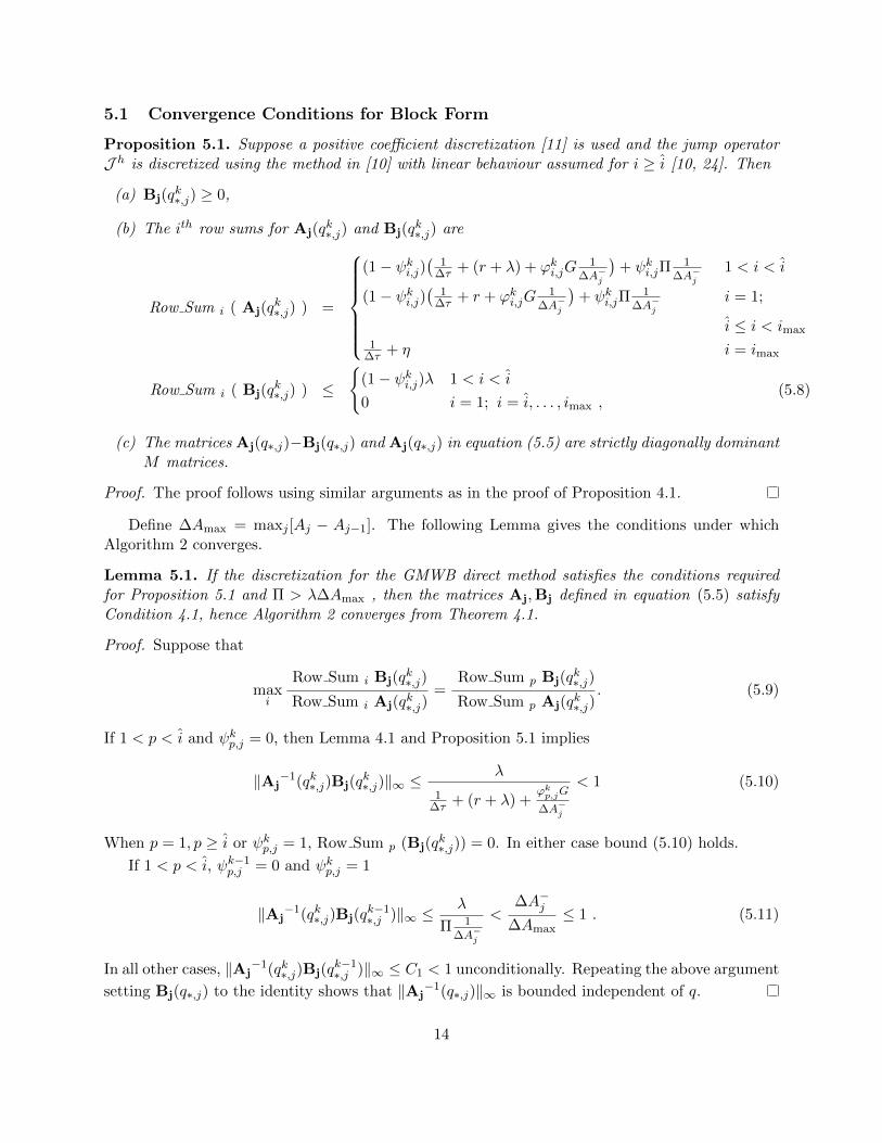
5.1 Convergence Conditions for Block Form
Proposition 5.1. Suppose a positive coefficient discretization [11] is used and the jump operatorJ h is discretized using the method in [10] with linear behaviour assumed for i ≥ i [10, 24]. Then
(a) Bj(qk∗,j) ≥ 0,
(b) The ith row sums for Aj(qk∗,j) and Bj(q
k∗,j) are
Row Sum i ( Aj(qk∗,j) ) =
(1− ψki,j)(
1∆τ + (r + λ) + ϕki,jG
1∆A−j
)+ ψki,jΠ
1∆A−j
1 < i < i
(1− ψki,j)(
1∆τ + r + ϕki,jG
1∆A−j
)+ ψki,jΠ
1∆A−j
i = 1;
i ≤ i < imax
1∆τ + η i = imax
Row Sum i ( Bj(qk∗,j) ) ≤
(1− ψki,j)λ 1 < i < i
0 i = 1; i = i, . . . , imax ,(5.8)
(c) The matrices Aj(q∗,j)−Bj(q∗,j) and Aj(q∗,j) in equation (5.5) are strictly diagonally dominantM matrices.
Proof. The proof follows using similar arguments as in the proof of Proposition 4.1.
Define ∆Amax = maxj [Aj − Aj−1]. The following Lemma gives the conditions under whichAlgorithm 2 converges.
Lemma 5.1. If the discretization for the GMWB direct method satisfies the conditions requiredfor Proposition 5.1 and Π > λ∆Amax , then the matrices Aj,Bj defined in equation (5.5) satisfyCondition 4.1, hence Algorithm 2 converges from Theorem 4.1.
Proof. Suppose that
maxi
Row Sum i Bj(qk∗,j)
Row Sum i Aj(qk∗,j)
=Row Sum p Bj(q
k∗,j)
Row Sum p Aj(qk∗,j)
. (5.9)
If 1 < p < i and ψkp,j = 0, then Lemma 4.1 and Proposition 5.1 implies
‖Aj−1(qk∗,j)Bj(q
k∗,j)‖∞ ≤
λ
1∆τ + (r + λ) +
ϕkp,jG
∆A−j
< 1 (5.10)
When p = 1, p ≥ i or ψkp,j = 1, Row Sum p (Bj(qk∗,j)) = 0. In either case bound (5.10) holds.
setting Bj(q∗,j) to the identity shows that ‖Aj−1(q∗,j)‖∞ is bounded independent of q.
14
Remark 5.1. Choosing a scaling factor which satisfies condition (iii) in Condition 4.1 means thatthis same scaling factor must be used in the optimization step in line 3 of Algorithm 1. Consequently,choosing different scaling factors will result, in general, in different choices for the control at eachiteration.
Remark 5.2. The fact that each Aj is a tridiagonal matrix simplifies the linear solving step ineach fixed-point policy iteration step. In particular, implementation of the block method is quitestraightforward.
6 Floating Point Considerations
6.1 Floating Point Considerations: General Results
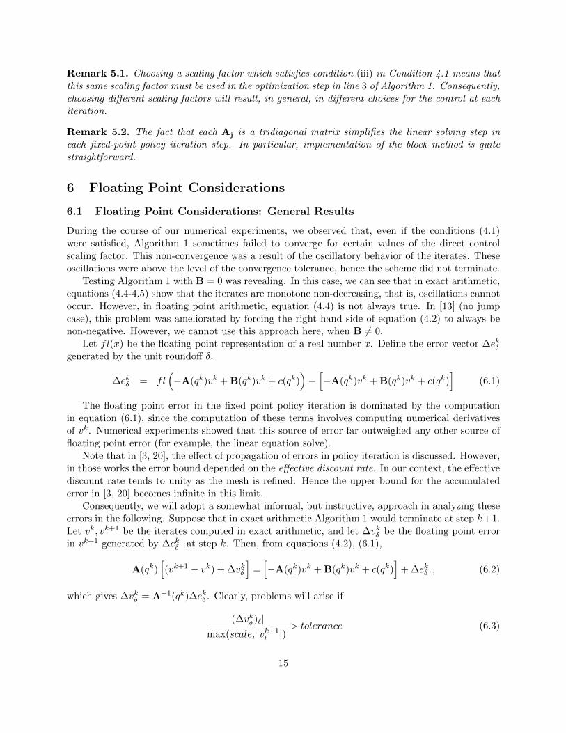
During the course of our numerical experiments, we observed that, even if the conditions (4.1)were satisfied, Algorithm 1 sometimes failed to converge for certain values of the direct controlscaling factor. This non-convergence was a result of the oscillatory behavior of the iterates. Theseoscillations were above the level of the convergence tolerance, hence the scheme did not terminate.
Testing Algorithm 1 with B = 0 was revealing. In this case, we can see that in exact arithmetic,equations (4.4-4.5) show that the iterates are monotone non-decreasing, that is, oscillations cannotoccur. However, in floating point arithmetic, equation (4.4) is not always true. In [13] (no jumpcase), this problem was ameliorated by forcing the right hand side of equation (4.2) to always benon-negative. However, we cannot use this approach here, when B 6= 0.
Let fl(x) be the floating point representation of a real number x. Define the error vector ∆ekδgenerated by the unit roundoff δ.
∆ekδ = fl(−A(qk)vk + B(qk)vk + c(qk)
)−[−A(qk)vk + B(qk)vk + c(qk)
](6.1)
The floating point error in the fixed point policy iteration is dominated by the computationin equation (6.1), since the computation of these terms involves computing numerical derivativesof vk. Numerical experiments showed that this source of error far outweighed any other source offloating point error (for example, the linear equation solve).
Note that in [3, 20], the effect of propagation of errors in policy iteration is discussed. However,in those works the error bound depended on the effective discount rate. In our context, the effectivediscount rate tends to unity as the mesh is refined. Hence the upper bound for the accumulatederror in [3, 20] becomes infinite in this limit.
Consequently, we will adopt a somewhat informal, but instructive, approach in analyzing theseerrors in the following. Suppose that in exact arithmetic Algorithm 1 would terminate at step k+1.Let vk, vk+1 be the iterates computed in exact arithmetic, and let ∆vkδ be the floating point errorin vk+1 generated by ∆ekδ at step k. Then, from equations (4.2), (6.1),
A(qk)[(vk+1 − vk) + ∆vkδ
]=[−A(qk)vk + B(qk)vk + c(qk)
]+ ∆ekδ , (6.2)
which gives ∆vkδ = A−1(qk)∆ekδ . Clearly, problems will arise if
|(∆vkδ )`|max(scale, |vk+1
` |)> tolerance (6.3)
15
since, even if |[(vk+1 − vk)
]`| is small, the iteration will not converge according to the criteria in
Algorithm 1.Consequently, we can estimate bounds for parameters that will minimize the effect of floating
point errors by requiring that
max`
[|(∆vkδ )`|
max(|vk+1` |, scale)
]= max
`
[[A−1(qk)∆ekδ ]`
max(|vk+1` |, scale)
]< tolerance . (6.4)
A rigorous bound for condition (6.4) is too pessimistic to be useful. We make the following approx-imation
max`
[[A−1(qk)∆ekδ ]`
max(|vk+1` |, scale)
]' max
`
[‖A−1(qk)‖∞|∆ekδ |`
max(|vk` |, scale)
], (6.5)
so that requirement (6.4) is estimated as
max`
[‖A−1(qk)‖∞|∆ekδ |`
max(|vk` |, scale)
]< tolerance . (6.6)
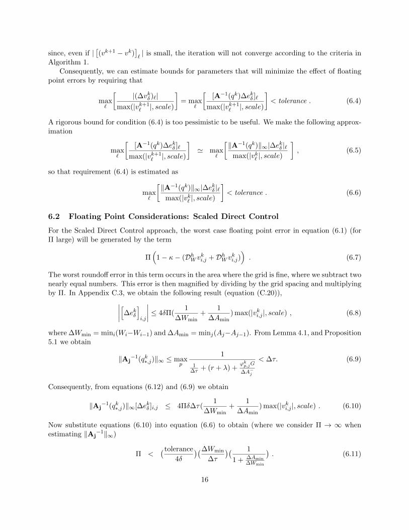
6.2 Floating Point Considerations: Scaled Direct Control
For the Scaled Direct Control approach, the worst case floating point error in equation (6.1) (forΠ large) will be generated by the term
Π(
1− κ− (DhW vki,j +DhW vki,j)). (6.7)
The worst roundoff error in this term occurs in the area where the grid is fine, where we subtract twonearly equal numbers. This error is then magnified by dividing by the grid spacing and multiplyingby Π. In Appendix C.3, we obtain the following result (equation (C.20)),∣∣∣∣[∆ekδ]i,j
∣∣∣∣ ≤ 4δΠ(1
∆Wmin+
1
∆Amin) max(|vki,j |, scale) , (6.8)
where ∆Wmin = mini(Wi−Wi−1) and ∆Amin = minj(Aj−Aj−1). From Lemma 4.1, and Proposition5.1 we obtain
‖Aj−1(qk∗,j)‖∞ ≤ max
p
1
1∆τ + (r + λ) +
ϕkp,jG
∆A−j
< ∆τ. (6.9)
Consequently, from equations (6.12) and (6.9) we obtain
‖Aj−1(qk∗,j)‖∞[∆ekδ ]i,j ≤ 4Πδ∆τ(
1
∆Wmin+
1
∆Amin) max(|vki,j |, scale) . (6.10)
Now substitute equations (6.10) into equation (6.6) to obtain (where we consider Π → ∞ whenestimating ‖Aj
−1‖∞)
Π <(tolerance
4δ
)(∆Wmin
∆τ
)( 1
1 + ∆Amin∆Wmin
). (6.11)
16
Conversely, if Π is small, then the worst case floating point error will be generated by the term12σ
2W 2i DhWWV
n+1i,j in equation (3.1), since this term involves a numerical second derivative. (See
the definition of L in equation (2.6)). From the result in Appendix C, equation (C.21), we have
|(∆ekδ )i,j | ≤ 4δσ2W 2
i
(∆Wmin)2i
max(scale, |vi,j |) , (6.12)
where (∆Wmin)i = min(Wi+1 − Wi,Wi − Wi−1). From Lemma 4.1, using Proposition 5.1, andconsidering the case where Π→ 0, we obtain
‖Aj−1(qk∗,j)‖∞ ≤ ∆Amax
Π(6.13)
where ∆Amax = maxj(Aj −Aj−1). Substituting (6.12) and (6.13) into (6.6) then gives
Π > 4σ2∆Amax
(W 2i
(∆Wmin)2i
)(δ
tolerance
), (6.14)
where
maxi
(W 2i
(∆Wmin)2i
)=
W 2i
(∆Wmin)2i
. (6.15)
Combining equation Lemma 5.1 and (6.14) we obtain
Π > max
[λ∆Amax, 4σ2∆Amax
(W 2i
(∆Wmin)2i
)(δ
tolerance
)]. (6.16)
In order to later compare the scaled direct control method with the penalty method [9, 13], letC∗ be the dimensionless constant
Π = C∗ω0
∆τ. (6.17)
The upper and lower bounds of C∗ for the scaled direct control method are then (from equations(6.11), (6.16), (6.17)),
C∗ > max
[λ∆Amax∆τ
ω0, 4
(σ2∆Amax∆τ
ω0
)(W 2i
(∆Wmin)2i
)(δ
tolerance
)],
C∗ <1
4
(tolerance
δ
)(∆Wmin
∆ω0
)(1
1 + ∆Amin∆Wmin
). (6.18)
7 Numerical Results
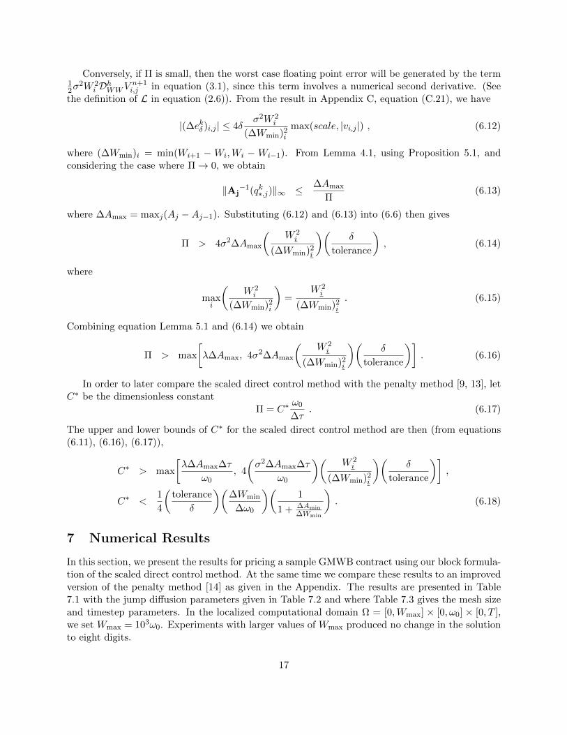
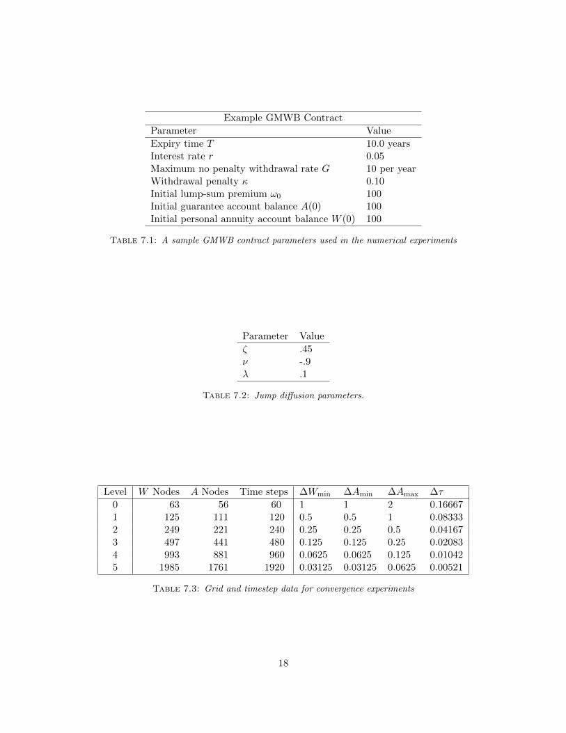
In this section, we present the results for pricing a sample GMWB contract using our block formula-tion of the scaled direct control method. At the same time we compare these results to an improvedversion of the penalty method [14] as given in the Appendix. The results are presented in Table7.1 with the jump diffusion parameters given in Table 7.2 and where Table 7.3 gives the mesh sizeand timestep parameters. In the localized computational domain Ω = [0,Wmax] × [0, ω0] × [0, T ],we set Wmax = 103ω0. Experiments with larger values of Wmax produced no change in the solutionto eight digits.
17
Example GMWB Contract
Parameter Value
Expiry time T 10.0 yearsInterest rate r 0.05Maximum no penalty withdrawal rate G 10 per yearWithdrawal penalty κ 0.10Initial lump-sum premium ω0 100Initial guarantee account balance A(0) 100Initial personal annuity account balance W (0) 100
Table 7.1: A sample GMWB contract parameters used in the numerical experiments
Parameter Value
ζ .45ν -.9λ .1
Table 7.2: Jump diffusion parameters.
Level W Nodes A Nodes Time steps ∆Wmin ∆Amin ∆Amax ∆τ
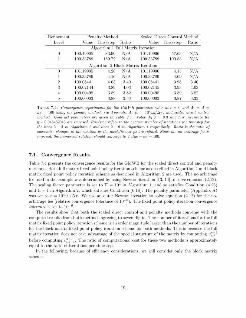
Table 7.4: Convergence experiments for the GMWB guarantee value at t = 0 and W = A =ω0 = 100 using the penalty method, see Appendix A, (ε = 104ω0/∆τ) and scaled direct controlmethod. Contract parameters are given in Table 7.1. Volatility σ = 0.3 and fair insurance feeη = 0.045452043 are imposed. Itns/step refers to the average number of iterations per timestep forthe lines 2 − 4 in Algorithm 2 and lines 2 − 9 in Algorithm 1 respectively. Ratio is the ratio ofsuccessive changes in the solution as the mesh/timesteps are refined. Since the no-arbitrage fee isimposed, the numerical solution should converge to V alue = ω0 = 100.
7.1 Convergence Results
Table 7.4 presents the convergence results for the GMWB for the scaled direct control and penaltymethods. Both full matrix fixed point policy iteration scheme as described in Algorithm 1 and blockmatrix fixed point policy iteration scheme as described in Algorithm 2 are used. The no arbitragefee used in the example was determined by using Newton iteration [13, 14] to solve equation (2.12).The scaling factor parameter is set to Π = 103 in Algorithm 1, and so satisfies Condition (4.26)and Π = 1 in Algorithm 2, which satisfies Condition (6.18). The penalty parameter (Appendix A)was set to ε = 104ω0/∆τ . We use an outer Newton iteration to solve equation (2.12) for the no-arbitrage fee (relative convergence tolerance of 10−8). The fixed point policy iteration convergencetolerance is set to 10−6.
The results show that both the scaled direct control and penalty methods converge with thecomputed results from both methods agreeing to seven digits. The number of iterations for the fullmatrix fixed point policy iteration scheme is an order magnitude larger than the number of iterationsfor the block matrix fixed point policy iteration scheme for both methods. This is because the fullmatrix iteration does not take advantage of the special structure of the matrix by computing vn+1
∗,jbefore computing vn+1
∗,j−1. The ratio of computational cost for these two methods is approximatelyequal to the ratio of iterations per timestep.
In the following, because of efficiency considerations, we will consider only the block matrixscheme.
19
7.2 Effect of Scaling Factor Π and Penalty Parameter ε [13]
In Section 6.2, we expressed the scaling factor Π in terms of a dimensionless parameter C∗ as in(6.17). Note that the scaled direct control method does not require the existence of a constantC such that 1/Π = C∆τ (see [13] for details). Writing Π = C∗ω0/∆τ is only for the purpose ofcomparing the scaled direct control method with the penalty method.
We refer to the bound on C∗ imposed by effect of floating point arithmetic as a Type I bound.The bound on C∗ imposed by requiring that ‖A−1(qk)B(qk−1)‖∞ < 1, will be referred to as a TypeII bound.
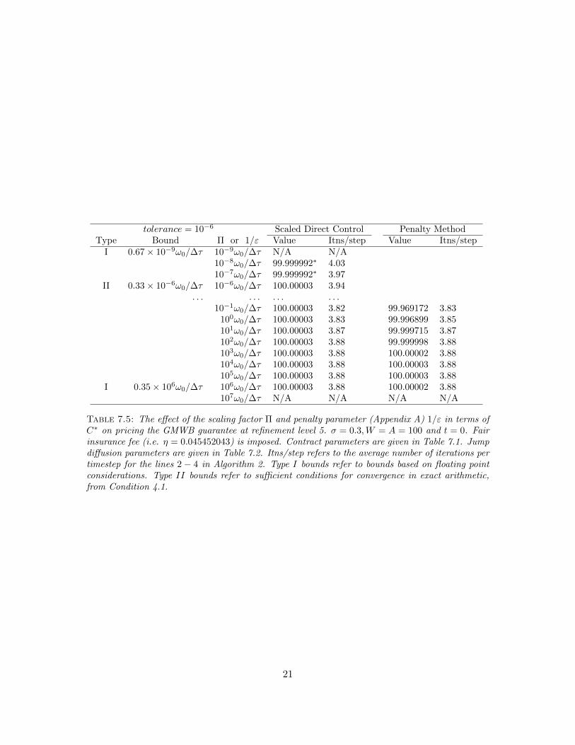
Table 7.5 compares the GMWB value priced by both scaled direct control and penalty methodswhen C∗ ∈ [10−9, 107]. The left two columns show the estimated bounds of C∗ from equations(A.15) and (6.18). Recall the definition of i from equation (6.15). The finest grids are around node(W = 100, A = 100), so we set Wi = 100, in the estimate of the floating point errors in equation(6.18). We take double precision machine epsilon to be δ = 1.11 × 10⁻¹⁶. The ”N/A” entries inthe table indicate that the iterative scheme did not satisfy the convergence criteria in Algorithm 1after 6000 iterations.
For the entries where the computed values have asterisks, although the convergence criterion inline 3 of Algorithm 1 was satisfied, we view these results as unreliable. Note that the convergencecriterion in Algorithm 1 is not able to clearly distinguish between very slowly diverging sequencesand truly converging sequences. We remind the reader that the Type II bound from Lemma 5.1 isa sufficient condition for convergence in exact arithmetic, from Condition 4.1. However, choosing aC∗ smaller than the estimated lower bound of C∗ from bound (6.18) produces questionable results.It is obvious the values with asterisks deviate somewhat from the other values.
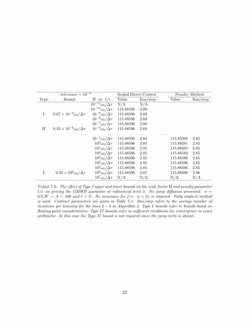
In the previous numerical examples, the lower bound for the scaling factor Π is dominated by aType II bound. To see the effect of Type I lower bound in isolation, we remove the jump diffusionfrom the underlying asset model (e.g. λ = 0). Consequently, ‖A−1(qk)B(qk−1)‖∞ < 1 always holdssince B(qk) = 0 for all k and hence the Type II bound disappears.
Table 7.6 shows the GMWB values priced at refinement level 5 (λ = 0). Without the presenceof Type II bound, we can further decrease the scaling factor by three orders of magnitude. Theestimated Type I lower bound for C∗ is remarkably close to the experimental result.
Remark 7.1 (Range of Values). These examples clearly show that the range of useful values of thescaling parameter for the scaled direct control method is much larger than the range of useful valuesfor the penalty parameter in the penalty method.
In Appendix D, we report some further numerical experiments which confirm that our estimatesfor the upper and lower bounds for the scaling factor are of the correct order.
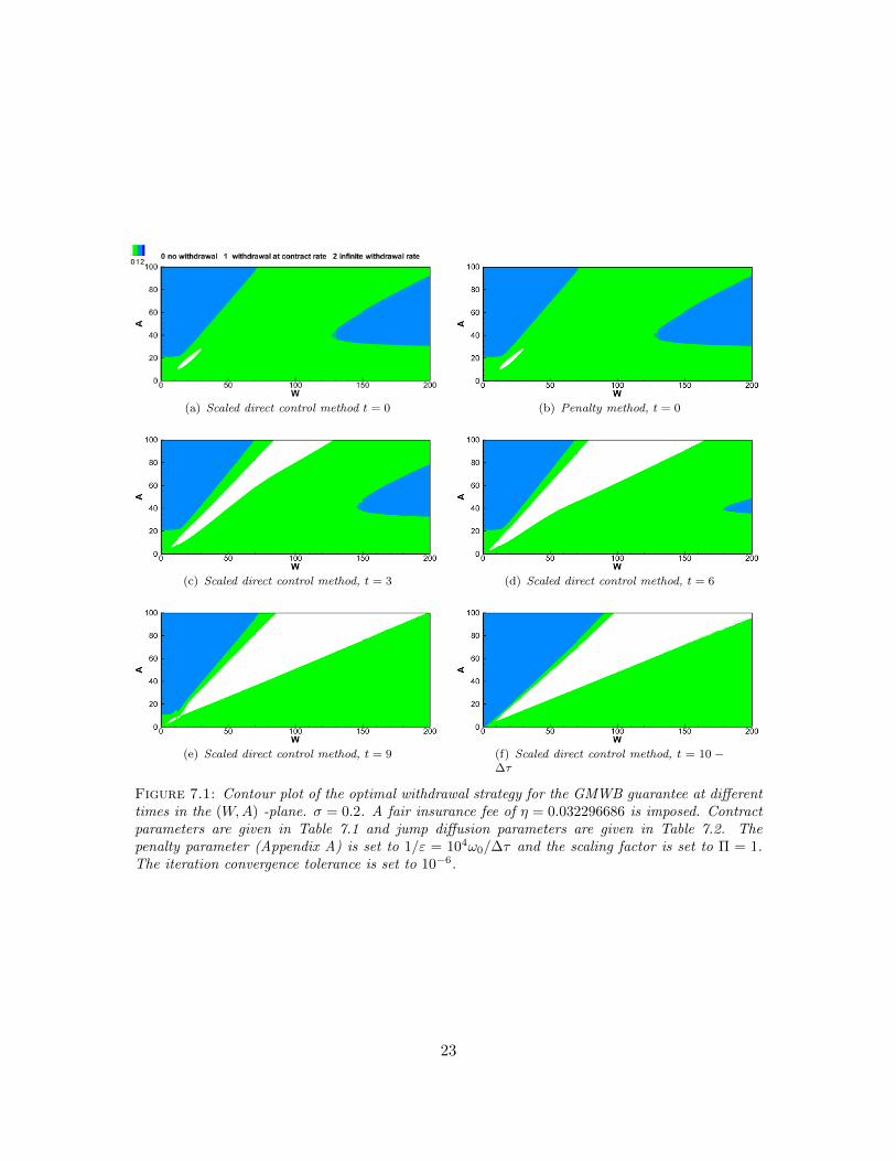
A GMWB contract holder is perhaps more interested in the optimal withdrawal strategy. Figure7.1 shows contour plots of the optimal withdrawal strategy at various times. The top two plots inFigure 7.1 are generated by both the scaled direct control and penalty methods. It can be observedthat these contour plots are very similar.
The other plots in Figure 7.1 are generated by the scaled direct control method. It is interestingto observe that the top left corner infinite withdrawal region is almost time-invariant, except whenthe contract is close to expiration. The no withdrawal region widens as time moves forward. Theseresults are consistent with the discrete withdrawal computations in [7].
20
tolerance = 10−6 Scaled Direct Control Penalty MethodType Bound Π or 1/ε Value Itns/step Value Itns/step
I 0.67× 10⁻⁹ω0/∆τ 10−9ω0/∆τ N/A N/A10−8ω0/∆τ 99.999992∗ 4.0310−7ω0/∆τ 99.999992∗ 3.97
Table 7.5: The effect of the scaling factor Π and penalty parameter (Appendix A) 1/ε in terms ofC∗ on pricing the GMWB guarantee at refinement level 5. σ = 0.3,W = A = 100 and t = 0. Fairinsurance fee (i.e. η = 0.045452043) is imposed. Contract parameters are given in Table 7.1. Jumpdiffusion parameters are given in Table 7.2. Itns/step refers to the average number of iterations pertimestep for the lines 2 − 4 in Algorithm 2. Type I bounds refer to bounds based on floating pointconsiderations. Type II bounds refer to sufficient conditions for convergence in exact arithmetic,from Condition 4.1.
21
tolerance = 10−6 Scaled Direct Control Penalty MethodType Bound Π or 1/ε Value Itns/step Value Itns/step
10−11ω0/∆τ N/A N/A10−10ω0/∆τ 115.88596 2.69
I 0.67× 10⁻⁹ω0/∆τ 10−9ω0/∆τ 115.88596 2.6910−8ω0/∆τ 115.88596 2.6910−7ω0/∆τ 115.88596 2.69
Table 7.6: The effect of Type I upper and lower bounds on the scale factor Π and penalty parameter1/ε on pricing the GMWB guarantee at refinement level 5. No jump diffusion presented. σ =0.3,W = A = 100 and t = 0. No insurance fee (i.e. η = 0) is imposed. Fully implicit methodis used. Contract parameters are given in Table 7.1. Itns/step refers to the average number ofiterations per timestep for the lines 2 − 4 in Algorithm 2. Type I bounds refer to bounds based onfloating point considerations. Type II bounds refer to sufficient conditions for convergence in exactarithmetic. In this case the Type II bound is not required since the jump term is absent.
22
(a) Scaled direct control method t = 0 (b) Penalty method, t = 0
(c) Scaled direct control method, t = 3 (d) Scaled direct control method, t = 6
(e) Scaled direct control method, t = 9 (f) Scaled direct control method, t = 10 −∆τ
Figure 7.1: Contour plot of the optimal withdrawal strategy for the GMWB guarantee at differenttimes in the (W,A) -plane. σ = 0.2. A fair insurance fee of η = 0.032296686 is imposed. Contractparameters are given in Table 7.1 and jump diffusion parameters are given in Table 7.2. Thepenalty parameter (Appendix A) is set to 1/ε = 104ω0/∆τ and the scaling factor is set to Π = 1.The iteration convergence tolerance is set to 10−6.
23
8 Conclusions
In this paper, we have carried out a systematic study of a scaled direct control iterative method forsolution of the GMWB pricing problem formulated as a singular control problem. The underlyingasset is assumed to follow a jump diffusion process.
We represent the discretized equations for the direct control technique using the general formof controlled HJB equations as in [14]. Sufficient conditions for convergence for a fixed point policyiteration are determined. A scaling factor is introduced in the direct control method.
The equations resulting from the singular control formation have a special structure that cansignificantly improve the efficiency of solving the resulting nonlinear system. A block matrix fixedpoint policy iteration scheme is given and the conditions required for convergence are determined.Numerical results show that this method is an order of magnitude better in terms of number ofiterations compared to a full matrix formulation.
In order to compare the method to the penalty method of [14] we also present a block versionof the penalty method and give conditions on when this method converges. Numerical experimentswere then done to compare both methods (both in block and non-block forms). The experimentsshow that the block methods are considerably more efficient in both cases.
Both the direct control and the penalty method technique requires specification of a parameter.This parameter affects both convergence and accuracy. We have estimated bounds for these param-eters for both methods, so that convergence in floating point arithmetic can be expected. To thebest of our knowledge, such analysis has not been carried out previously. Numerical experimentsindicate that these estimates are reasonably accurate.
From a practical perspective, it is safe to choose the dimensionless penalty parameter and thedimensionless direct control scaling factor two orders of magnitude away from the estimated upperbounds.
It would appear that the order of magnitude useful range of the scaling parameter for the directcontrol method is much larger than the useful range for the penalty parameter in the penaltymethod. The accuracy and convergence rate for both methods is similar for parameters within theuseful range. Consequently, it would appear that the scaled direct control method is superior tothe penalty method in this regard.
Appendix
A The Penalty Method for solving the GMWB Problem
A penalty method for solving the singular GMWB problem under a jump diffusion process hasbeen given in [14]. The penalized form is formulated as
V ετ = LV ε + λJ V ε + max
ϕ∈0,1,ψ∈0,1ϕψ=0
[ϕGFV ε + ψ
((FV ε − κ)
ε+ κG
)]. (A.1)
or equivalently
V ετ − λJ V ε + min
ϕ∈0,1,ψ∈0,1ϕψ=0
[−LV ε − ϕGFV ε − ψ
((FV ε − κ)
ε+ κG
)]= 0. (A.2)
24
The basic idea of the penalty method is to discretize equation (A.1), and let the penalty parameterε→ 0 as the mesh and timesteps tend to zero.
In [14] the penalty method was discretized with a fully implicit method and a fixed point policyiteration method was given to solve the resulting nonlinear algebraic equations. The key in thiscase was to show that the discretization satisfied Condition 4.1.
We wish to compare the direct control method with the penalty method. In order to do thiswe require a block form of the penalty form and an analysis of the floating point behaviour of theblock form algorithm.
A.1 Block Form for the Singular Control GMWB Penalty Method
As discussed in [13, 14], with ε = C∆τ and C a constant, the final discretized form of (A.1) forthe penalty method becomes
1
∆τV n+1i,j − LhV n+1
i,j + ϕ∗i,jG(DhAV n+1i,j +DhWV n+1
i,j ) +ψ∗i,jε
(DhAV n+1i,j +DhWV n+1
i,j )
= λ[J hV n+1]i,j + ϕ∗i,jG+ ψ∗i,j(1− κε
+ κG) +1
∆τV ni,j (A.3)
where
ϕ∗i,j , ψ∗i,j ∈ arg maxϕ∈0,1,ψ∈0,1
ϕψ=0
ϕ G(1−Dh
AVn+1i,j −DhWV n+1
i,j )
+ ψ(1−DhAV
n+1i,j −Dh
WVn+1i,j − κ
ε+ κG
). (A.4)
Equation (A.3) can also be rewritten in an equivalent form (replacing DhA by a backward difference)
1
∆τV n+1i,j − LhV n+1
i,j + ϕ∗i,jG(V n+1i,j
∆A−j+DhWV n+1
i,j ) +ψ∗i,jε
(V n+1i,j
∆A−j+DhWV n+1
i,j )
= λ[J hV n+1]i,j + ϕ∗i,jG+ ψ∗i,j(1− κε
+ κG) +1
∆τV ni,j
+(ϕ∗i,jG+ψ∗i,jε
)1
∆A−jV n+1i,j−1 (A.5)
The boundary conditions are similar to the direct control case.In this subsection we describe a block form for (A.5) and (3.5). Let u = ((u∗,1)′, (u∗,2)′, . . . , (u∗,jmax)′)′
be an N length vector. The imax × imax square matrices Aj,Bj and the vector c∗,j of size imax are
Remark A.1. We have written the matrix Bj = Bjk although there is no explicit dependence on
(ϕk∗,j , ψk∗,j) in this case in order to use the general form of the earlier sections.
In order to ensure convergence to the viscosity solution of equation (2.5), the discretizationmust be monotone, consistent and l∞ stable [2]. A positive coefficient discretization guaranteesmonotonicity [11]. The positive coefficient condition and the discretization of the jump term as in[10] give the following result.
Proposition A.1. Suppose a positive coefficient discretization [11] is used and the jump operatorJ hj is discretized using the method in [10], with linear behaviour assumed for i ≥ i [10, 24]. Then
(a) Bj(qk∗,j) ≥ 0,
(b) The ith row sums for Aj(qk∗,j) and Bj(q
k∗,j) are
Row Sum i ( Aj(qk∗,j) ) =
1
∆τ + (r + λ) + (ϕki,jG+ψki,j
ε ) 1∆A−j
1 < i < i
1∆τ + r + (ϕki,jG+
ψki,j
ε ) 1∆A−j
i = 1; i = i, ..., imax − 1
1∆τ + η i = imax
Row Sum i ( Bj(qk∗,j) ) ≤
λ 1 < i < i
0 i = 1; i = i, ..., imax
(A.9)
26
(c) The matrices Aj(q∗,j)−Bj(q∗,j) and Aj(q∗,j) in equation (A.8) are strictly diagonally domi-nant M matrices.
Proof. (a) and the second part of (b) follow in similar fashion as in the proof of Proposition 4.1.In order to prove the remaining part of (b) we note that the row sum is the same as [Aj(q
k∗,j)e]i
with e = (1, ..., 1)′. Noting properties (4.10), we see that [Aj(qk∗,j)e]i = 1
∆τ + (r + λ) + (ϕki,jG +ψki,j
ε ) 1∆A−j
for i < i. A similar argument shows that [Aj(qk∗,j)e]i = 1
∆τ + r + (ϕki,jG +ψki,j
ε ) 1∆A−j
for
i ≤ i < imax or i = 1. When i = imax then from the boundary assignment of equation (3.5), its rowsum is just (1/∆τ + η).
To prove (c), note that Aj and (Aj − Bj) have non-positive off-diagonals (since a positivecoefficient discretization is used [11]). From (b), the row sums of (Aj−Bj), Aj are strictly positive.Hence Aj and (Aj −Bj) are M matrices [23].
The convergence result for the block matrix method, using the penalty formulation, is then:
Lemma A.1. Assume that the discretization for the GMWB penalty method satisfies the conditionsrequired for Proposition A.1. Then the matrices Aj,Bj satisfy Condition 4.1, and hence fromTheorem 4.1, Algorithm 2 converges.
Proof. Because Bj(qk∗,j) is independent of qk∗,j , we only need to show that
‖Aj−1(qk∗,j)Bj(q
k∗,j)‖∞ ≤ C1 (A.10)
for some constant C1 < 1. From Lemma 4.1 and Proposition A.1, it follows that
‖Aj−1(qk∗,j )Bj(q
k∗,j )‖∞ ≤ max
i,j
[λ
1∆τ + (r + λ) + (ϕki,jG+
ψki,j
ε ) 1∆A−j
]< 1. (A.11)
By setting Bj = I, we obtain immediately that Aj−1(qk∗,j ) is bounded independent of q.
A.2 Floating Point Considerations: Block Penalty Method
For the penalty method, the floating point error of each iteration is dominated by computation ofthe following term in equation (6.1)
1
ε
(1− κ− (DhW vki,j +DhW vki,j)
). (A.12)
As done in Subsection 6.2, we can then estimate
4δ∆τ
ε(
1
∆Wmin+
1
∆Amin) < tolerance . (A.13)
In order to ensure that the penalty method is consistent with the original HJB variationalinequality, we require that the penalty parameter ε = C∆τ for any constant C > 0 [13]. Intuitively,1/ε is the maximum withdrawal rate, so that it has dimensions of currency/time.
Define a dimensionless constant C∗ such that
1
ε= C∗
ω0
∆τ. (A.14)
27
Substituting equation (A.14) into equation (A.13)
C∗ <1
4
(tolerance
δ
)(∆Wmin
ω0
)(1
1 + ∆Wmin∆Amin
). (A.15)
See [13] for the financial intuition for selecting this form for C∗.
B Finite Difference Approximation
B.1 First and second derivatives approximation
In this Appendix, we use a standard finite difference method to approximate the first and secondpartial derivatives in the PDE. The discretized differential operators DhA, DhW and DhWW are givenby
DhAV ni,j =
V ni,j − V n
i,j−1
∆A−j, backward differencing,
DhWV ni,j =
V ni,j−V n
i−1,j
∆W−ibackward differencing,
V ni+1,j−Vi,j
∆W+i
forward differencing,V ni+1,j−V n
i−1,j
∆W±icentral differencing,
DhWWVni,j =
V ni−1,j−V n
i,j
∆W−i+
V ni+1,j−V n
i,j
∆W+i
∆W±i2
=DhWV n
i+1,j −DhWV ni,j
∆W±i2
(DhW is backward differenced). (B.1)
where ∆A−j = Aj −Aj−1, ∆W−i = Wi−Wi−1, ∆W+i = Wi+1−Wi, and ∆W±i = Wi+1−Wi−1.
Together with the boundary condition (2.11), the discretized Lh and Fh [13] operators are
LhV ni,j =
σ2
2 W2i DhWWV
ni,j + (r − η)WiDhWV n
i,j − rV ni,j , (Wi, Aj , τ
n) ∈ Ωin ∪ ΩA0
−rV ni,j , (Wi, Aj , τ
n) ∈ ΩW0
, (B.3)
FhV ni,j =
1−DhWV n
i,j −DhAV ni,j , (Wi, Aj , τ
n) ∈ Ωin
1−DhAV ni,j , (Wi, Aj , τ
n) ∈ ΩW0
0, (Wi, Aj , τn) ∈ ΩA0
. (B.4)
28
C Floating Point Arithmetic Error Analysis
C.1 Roundoff Error Propagation
Let x = (x1, x2, . . . , xn)′ to compute a function y = φ(x) by using floating point arithmetic, anerror ∆y of yδ0 has to be expected, where |δ0| < δ, the machine epsilon [21]. Further more, thereexists an input error ∆x = (∆x1,∆x2, . . . ,∆xn)′ due to the floating point representation of realnumbers or previous calculation of x (we do not consider the measurement input error because itis beyond the control of numerical computation method). The two sources of error are unavoidableno matter how we arrange the floating point operations. The third source of error comes from theintermediate roundoff errors and it depends how we arrange the floating point operations. Basedon differential error analysis, the total floating point arithmetic error of computing y denoted by∆y, to the first order approximation, is given by
∆y = Dφ(x)∆x+ yδ0 +r∑i=1
∆(i)y (C.1)
with Dφ(x) being the Jacobian matrix of φ(x) and ∆(i)y being the intermediate roundoff errorgenerated at step i. We assume there are r intermediate steps and each step performs elementaryoperations such as +,−,×,÷ and
√[21].
C.2 Derivative Roundoff Error by Finite Difference
Using the standard finite difference method to compute the first derivative involves floating pointarithmetic of computing the function with form
y = φ1(x) =x1 − x2
x3. (C.2)
Let the input relative error be denoted by δx = (δx1 , δx2 , δx3)′ = (∆x1/x1,∆x2/x2,∆x3/x3)′,If we compute y1 = x1 − x2 first, then proceed to divide the intermediate result y1 by x3, fromequation (C.1), we have
∆y = δx1x1
x3− δx2
x2
x3− δx3y + δ0y + δ1y
where |δi| < δ(i = 1, 2) and δ1y is the intermediate roundoff error. Further assuming |δx3 | ≤ δ and|x3| ≤ ∆hmin, we obtain the bound of ∆y as follows
Suppose input error ∆x is due to representing the real number in floating point system or previouscalculation whose error is within machine epsilon δ, so we have ‖δx‖∞ ≤ δ and consequently
|∆y| ≤ δ(2 + 4|ai|)|xi|
∆hmini = 1, 2 . (C.6)
Apply the result to discretized DhWVn+1i,j and DhAV
n+1i,j in equation (B.1), we obtain the absolute
roundoff error of computing first derivatives by using backward difference as follows
|∆DhAV n+1i,j | ≤ δ(2 + 4|a3|)
|V n+1i,j |
∆A−j, V n+1
i,j−1 = (1 + a3)V n+1i,j
|∆DhWV n+1i,j | ≤ δ(2 + 4|a4|)
|V n+1i,j |
∆W−i, V n+1
i−1,j = (1 + a4)V n+1i,j
|∆DhWV n+1i+1,j | ≤ δ(2 + 4|a5|)
|V n+1i,j |
∆W−i, V n+1
i+1,j = (1 + a5)V n+1i,j (C.7)
Apply the result in equation (C.5) to DhAVi,j , DhWVi,j and DhWVn+1i+1,j , we have
|DhAV n+1i,j | ≤ |a3|
|V n+1i,j |
∆A−j, |DhWV n+1
i,j | ≤ |a4||V n+1i,j |
(∆Wmin)i, |DhWV n+1
i+1,j | ≤ |a5||V n+1i,j |
(∆Wmin)i,(C.8)
where (∆Wmin)i = min(Wi+1−Wi,Wi−Wi−1). Together with the standard 3 point finite differencemethod to compute the second derivative as in equation (B.1) , we obtain
|DhWWVn+1i,j | ≤ (|DhWV n+1
i+1,j |+ |DhWV
n+1i,j |)
1
(∆Wmin)i
≤ (|a4|+ |a5|)|V n+1i,j |
(∆Wmin)2i
. (C.9)
To bound the roundoff error of DhWWVn+1i,j , set
x = (DhWV n+1i+1,j ,D
hWV
n+1i,j ,
∆W±i2
)′ , δx = (∆DhWV
n+1i+1,j
DhWVn+1i+1,j
,∆DhWV
n+1i,j
DhWVn+1i,j
, δx3)′ . (C.10)
Assuming |δx3 | < δ, by equations (B.1), (C.3), (C.8) and (C.9) and the fact that ∆W±i /2 ≥∆(Wmin)i, we obtain the following bound
|∆DhWWVn+1i,j | ≤
|∆DhWVn+1i,j |+ |∆DhWV
n+1i+1,j |
(∆Wmin)i+ 3|DhWWV
n+1i,j |
≤ δ(4 + 5|a4|+ 5|a5|)|V n+1i,j |
(∆Wmin)2i
(C.11)
C.3 Roundoff Error Estimation of Local Optimization Problem
During each iteration, we solve local optimization problem and the objective function involvescalculating the following two terms
f1(Wi, Aj , τn+1) = κ− 1 +DhWV n+1
i,j +DhAV n+1i,j (C.12)
f2(Wi, Aj , τn+1) =
σ2W 2i
2DhWWV
n+1i,j +O(Wi) . (C.13)
30
Computing f1 involves calculating a function of the form g(x) = (x1 + x2) + (x3 + x4). Fromequation (C.1), we obtain
|∆g| ≤4∑i=1
|∆xi|+ δ|g|+ δ|x1 + x2|+ δ|x3 + x4| (C.14)
≤4∑i=1
|∆xi|+ 2δ|x1 + x2|+ 2δ(|x3|+ |x4|) . (C.15)
Set x1 = κ, x2 = −1, x3 = DhWVn+1i,j , x4 = DhAV
n+1i,j and apply equations (C.7) and (C.8) with the
fact that 0 < κ < 1, we obtain the bound of absolute roundoff error of f1 as follows
|∆f1| ≤ δ(2 + 6|a3|)|V n+1i,j |
∆A−j+ δ(2 + 6|a4|)
|V n+1i,j |
(∆Wmin)i+ 3(1− κ)δ
/ 2δ(1 + 3|a3|∆Amin
+1 + 3|a4|∆Wmin
)|V n+1i,j | , (C.16)
where we discard the smaller error term of 3δ(1 − κ), and ∆Amin = minj(Aj − Aj−1, ∆Wmin =mini(Wi −Wi−1).
To analyze the roundoff error of f2, we notice that only multiplication and division operationsare involved given DhWWV
n+1i,j as one of the operands. From equation (C.1), it can be easily seen
So computing of ci = σ2W 2i /2 will accumulate 9δ|ci| roundoff errors assuming the input error of
σ and Wi is smaller than δ, the machine epsilon. The final roundoff error of f2 = ciDhWWVn+1i,j is
then given by
|∆f2| ≤ (10|δ|+|∆DhWWV
n+1i,j |
|DhWWVn+1i,j |
)|ci||DhWWVn+1i,j |
≤ δ(4 + 15|a4|+ 15|a5|)σ2W 2
i
2(∆Wmin)2i
|V n+1i,j | (C.19)
In the area where the grids are fine, we have Vi,j ≈ Vi±1,j ≈ Vi,j−1. So normally |ai| 1 fori = 3, 4, 5. It may be safe to estimate that |ai| ≤ 0.1, i = 3, 4, 5. Finally the following estimation ofroundoff errors of computing f1 and f2 are obtained.
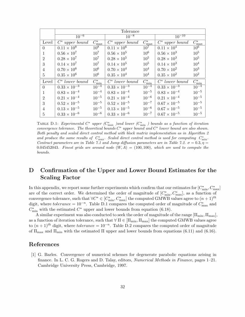
min ) bounds as a function of iterationconvergence tolerance. The theoretical bounds C∗ upper bound and C∗ lower bound are also shown.Both penalty and scaled direct control method with block matrix implementation as in Algorithm 2and produce the same results of C∗
max. Scaled direct control method is used for computing C∗min.
Contract parameters are in Table 7.1 and Jump diffusion parameters are in Table 7.2. σ = 0.3, η =0.045452043. Finest grids are around node (W,A) = (100, 100), which are used to compute thebounds.
D Confirmation of the Upper and Lower Bound Estimates for theScaling Factor
In this appendix, we report some further experiments which confirm that our estimates for [C∗min, C∗max]
are of the correct order. We determined the order of magnitude of [C∗min, C∗max], as a function of
convergence tolerance, such that ∀C∗ ∈ [C∗min, C∗max] the computed GMWB values agree to (n+ 1)th
digit, where tolerance = 10−n. Table D.1 compares the computed order of magnitude of C∗max andC∗min with the estimated C∗ upper and lower bounds from equation (6.18).
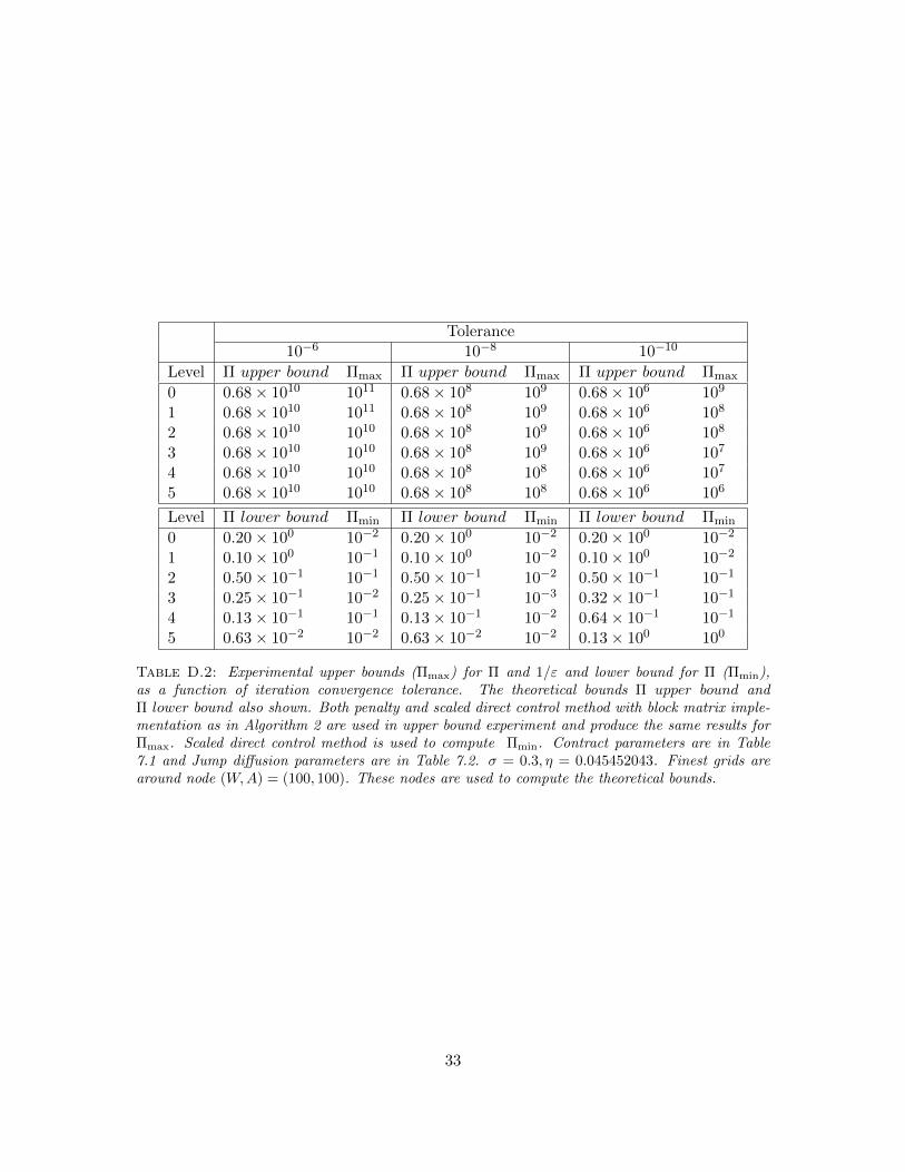
A similar experiment was also conducted to seek the order of magnitude of the range [Πmin,Πmax],as a function of iteration tolerance, such that ∀ Π ∈ [Πmin,Πmax] the computed GMWB values agreeto (n+ 1)th digit, where tolerance = 10−n. Table D.2 compares the computed order of magnitudeof Πmax and Πmin with the estimated Π upper and lower bounds from equations (6.11) and (6.16).
References
[1] G. Barles. Convergence of numerical schemes for degenerate parabolic equations arising infinance. In L. C. G. Rogers and D. Talay, editors, Numerical Methods in Finance, pages 1–21.Cambridge University Press, Cambridge, 1997.
Table D.2: Experimental upper bounds (Πmax) for Π and 1/ε and lower bound for Π (Πmin),as a function of iteration convergence tolerance. The theoretical bounds Π upper bound andΠ lower bound also shown. Both penalty and scaled direct control method with block matrix imple-mentation as in Algorithm 2 are used in upper bound experiment and produce the same results forΠmax. Scaled direct control method is used to compute Πmin. Contract parameters are in Table7.1 and Jump diffusion parameters are in Table 7.2. σ = 0.3, η = 0.045452043. Finest grids arearound node (W,A) = (100, 100). These nodes are used to compute the theoretical bounds.
33
[2] G. Barles and P.E. Souganidis. Convergence of approximation schemes for fully nonlinearequations. Asymptotic Analysis, 4:271–283, 1991.
[3] D.P. Bertsekas and J. Tsitsiklis. Neuro-dynamic Programming. Athena, 1996.
[4] O. Bokanowski, S. Maroso, and H. Zidani. Some convergence results for Howard’s algorithm.SIAM Journal on Numerical Analysis, 47:3001–3026, 2009.
[5] A. Budhriaja and K. Ross. Convergent numerical scheme for singular stochastic control withstate constraints in a portfolio selection problem. SIAM Journal on Control and Optimization,45:2169–2206, 2007.
[6] Z. Chen and P. A. Forsyth. A numerical scheme for the impulse control formulation for pricingvariable annuities with a guaranteed minimum withdrawal benefit (GMWB). NumerischeMathematik, 109:535–569, 2008.
[7] Z. Chen, K. Vetzal, and P.A. Forsyth. The effect of modelling parameters on the value ofGMWB guarantees. Insurance: Mathematics and Economics, 43:165–173, 2008.
[8] R. Cont and P. Tankov. Financial Modelling with Jump Processes. Chapman and Hall, 2004.
[9] M. Dai, Y. K. Kwok, and J. Zong. Guaranteed minimum withdrawal benefit in variableannuities. Mathematical Finance, 18:595–611, 2008.
[10] Y. d’Halluin, P.A. Forsyth, and K.R. Vetzal. Robust numerical methods for contingent claimsunder jump diffusion processes. IMA Journal of Numerical Analysis, 25:87–112, 2005.
[11] P. A. Forsyth and G. Labahn. Numerical methods for controlled Hamilton-Jacobi-BellmanPDEs in finance. Journal of Compuational Finance, 11 (Winter):1–44, 2008.
[12] A. Hindy, C. Huang, and S. Zhu. Numerical analysis of a free boundary singular controlproblem in financial economics. Journal of Economic Dynamics and Control, 21:297–327,1997.
[13] Y. Huang and P.A. Forsyth. Analysis of a penalty method for pricing a guaranteed minimumwithdrawal benefit (GMWB). Working paper, University of Waterloo, to appear in the IMAJournal of Numerical Analysis, 2010.
[14] Y. Huang, P.A. Forsyth, and G. Labahn. Combined fixed and point policy iteration for HJBequations in finance. Working paper, University of Waterloo, submitted to SIAM journal onNumerical Analysis, 2010.
[15] S. Kumar and K. Mithiraman. A numerical method for solving singular stochastic controlproblems. Operations Research, 52:563–582, 2004.
[16] H.J. Kushner and P.G Dupuis. Numerical Methods for Stochastic Control Problems in Con-tinupus Time. Springer-Verlag, New York, 1991.
[17] M. A. Milevsky and T. S. Salisbury. Financial valuation of guaranteed minimum withdrawalbenefits. Insurance: Mathematics and Economics, 38:21–38, 2006.
34
[18] H. Pham. On some recent aspects of stochastic control and their applications. ProbabilitySurveys, 2:506–549, 2005.
[19] D.M. Pooley, P.A. Forsyth, and K.R. Vetzal. Numerical convergence properties of optionpricing PDEs with uncertain volatility. IMA Journal of Numerical Analysis, 23:241–267, 2003.
[20] Munos R. Error bounds for approximate policy iteration. pages 560–567, 2003. Proceedingsof the 20th International Congress on Machine Learning, Washington.
[21] J. Stoer and R. Bulirsch. Introduction to Numerical Analysis. Springer-Verlag, second edition,1993.
[22] A. Tourin and T. Zariphopoulou. Viscosity solutions and numerical schemes for invest-ment/consumption models with transaction costs. in Numerical Methods in Finance, editors:L.C.G. Rogers and D. Talay, Cambridge University Press, 1997.
[23] R. Varga. Matrix Iterative Analysis. Prentice Hall, 1961.
[24] I.R. Wang, J.W.I. Wan, and P.A. Forsyth. Robust numerical valuation of European and Amer-ican options under the CGMY proces. Journal of Computational Finance, 10:4(Summer):86–115, 2007.
[25] J. Wang and P.A. Forsyth. Maximal use of central differencing for Hamilton-Jacobi-BellmanPDEs in finance. SIAM Journal on Numerical Analysis, 46:1580–1601, 2008.