Biostatistics (2019), 0, 0, pp. 1–27doi:10.1093/biostatistics/FMM˙fmri

A functional mixed model for scalar on function

regression with application to a functional MRI

study

Wanying Ma, Luo Xiao∗, Bowen Liu,

Department of Statistics, North Carolina State University, 2311 Stinson Drive, Raleigh, NC,

27606, USA

lxiao5@ncsu.edu

Martin A. Lindquist

Department of Biostatistics, Johns Hopkins Bloomberg School of Public Health, 615 N. Wolfe

Street, Baltimore, MD, 21205, USA

Summary

Motivated by a functional magnetic resonance imaging (MRI) study, we propose a new functional

mixed model for scalar on function regression. The model extends the standard scalar on function

regression for repeated outcomes by incorporating subject-specific random functional effects.

Using functional principal component analysis, the new model can be reformulated as a mixed

effects model and thus easily fit. A test is also proposed to assess the existence of the subject-

specific random functional effects. We evaluate the performance of the model and test via a

simulation study, as well as on data from the motivating fMRI study of thermal pain. The data

application indicates significant subject-specific effects of the human brain hemodynamics related

∗To whom correspondence should be addressed.

© The Author 2019. Published by Oxford University Press. All rights reserved. For permissions, please e-mail: journals.permissions@oup.com

2 W. Ma and others

to pain and provides insights on how the effects might differ across subjects.

Key words: Functional data analysis; Functional principal component; Functional mixed model; Repeated

measurements; fMRI; Variance component testing.

1. Introduction

Scalar on function regression models (Ramsay, 2006) are used to relate functional predictors to

scalar outcomes and are becoming increasingly popular in statistical applications (e.g., Goldsmith

and others, 2011; Morris, 2015; Reiss and others, 2017). These models have also been extended

to data with repeated outcomes (e.g., Goldsmith and others, 2012; Gertheiss and others, 2013).

However, existing models only model the effects of the functional predictor as fixed and do not

allow for random functional effects that are either subject- or outcome-specific.

We are motivated by a functional magnetic resonance imaging (fMRI) study of thermal pain

(Lindquist, 2012). We begin by briefly describing the study, which was performed on 20 partici-

pants. A number of stimuli, consisting of thermal stimulations delivered to the participants left

forearm, were applied at two different levels (high and low) to each participant. The temperature

of these painful (high) and non-painful (low) stimuli were determined using a pain calibration

task performed prior to the experiment. After an 18s time period of thermal stimulation (either

high or low), a fixation cross was presented for a 14s time period until the words “How painful?”

appeared on the screen. After four seconds of silent contemplation, participants rated the over-

all pain intensity on a visual analog scale (VAS). The ratings took continuous values and were

re-scaled within the range of 100 to 600. The experiment concluded with 10s of rest. During the

course of the experimental trial, each subject’s brain activity was also measured using fMRI.

Data was extracted from different known pain-responsive brain regions across the brain. Each

time course consisted of 23 equidistant measurements made every 2s, providing a total of 46s of

Functional mixed model for scalar on function regression 3

brain activation, ranging from the time of onset of the application of the stimuli to the conclusion

of the pain report. The same experiment was conducted multiple times on each participant, with

the total number of the repetitions ranging from 39 to 48, thereby giving rise to an unbalanced

design. To illustrate the structure of the data, Figure 1 shows the fMRI and the pain rating data

for two subjects each with three repetitions, mimicking Figure 1 in Goldsmith and others (2012).

In previous work, Lindquist (2012) used this data set to study how brain activation affected

the pain rating using a scalar on function regression model that treated the continuously observed

fMRI data as a functional covariate and the subjective rating as a scalar response. However, they

used a population model that did not allow for the subject-specific effect of the fMRI imaging on

the pain rating to be appropriately modeled. In this work, we seek to determine whether the fMRI

data affects the pain rating in a unified or subject-specific manner. For this purpose, we extend the

scalar on function linear regression to a new functional mixed effects model for repeated outcomes,

and develop a test to determine if the relation between the brain imaging data (more specifically,

fRMI data at one brain region) and the pain rating is subject-specific or not. Suggested by the

Associate Editor, we further extend the proposed model and test to simultaneously assess the

association between pain rating and fMRI data at multiple brain regions.

Testing for the lack of an effect in a functional predictor, i.e., whether the coefficient function

is exactly zero, has been well developed in the scalar on function regression literature. For exam-

ple, Cardot and others (2003) developed a test using the covariance of the scalar response and the

functional predictor. Swihart and others (2014) and McLean and others (2015) used the exact

likelihood ratio tests of zero variance components (Crainiceanu and Ruppert, 2004). Kong and

others (2016) proposed classical Wald, score and F-tests; see also Su and others (2017). However,

these tests all focus on fixed functional effects and hence are not applicable to simultaneously

testing a collection of random functional effects. Instead of directly testing if multiple random

functional effects are all zero, we propose an equivalent test, which tests if the covariance func-

4 W. Ma and others

tion of the random functional effects is zero or not. The test can be further formulated as testing

whether multiple variance components are zero. Because existing tests for multiple variance com-

ponents are either computationally intensive or conservative (Qu and others, 2013; Drikvandi

and others, 2012; Baey and others, 2019), we propose an alternative test which is based on the

exact likelihood ratio test of one zero variance component (Crainiceanu and Ruppert, 2004) and

can be more powerful for finite sample data.

The remainder of this paper is organized as follows. In Section 2, we describe our proposed

model along with model estimation and also our test. In Section 3, we extend the proposed model

to deal with a multivariate functional predictor. In Section 4, we assess the numerical performance

of our model and test. In Section 5, we consider the motivating data application. We conclude

the paper with some discussion in Section 6.

2. Method

2.1 Functional mixed model for scalar on function regression with repeated outcomes

We begin by introducing notation. For subject i (i = 1, 2, . . . , n = 20), let Yij denote the pain

rating at the jth repetition with j = 1, 2, . . . , ni and ni denotes the number of repetitions for

subject i. Similarly, let Zij denote the level of stimuli for the jth repetition for subject i, with

Zij = 1 representing high and Zij = 0 representing low. We shall first consider the fMRI time

series data at one brain region, which corresponds to a univariate functional predictor. In Section

3, we shall extend our model to fMRI data at multiple regions, which corresponds to a multivariate

functional predictor. Let Wijk denote the observed fMRI data at time tk = 2k seconds (k =

1, 2, . . . ,K = 23), which is assumed to be a noisy observation of the smooth functional data

Xij(tk). Let T = [0, 46] denote the time course of the experiment.

To model the subject-specific random effect of a functional predictor, we propose a new

functional mixed model extending the scalar on function linear regression for repeated outcomes.

Functional mixed model for scalar on function regression 5

The proposed model is

Yij = α+ αi + Zij(γ + γi) +

∫t∈T{β(t) + Zijδ(t) + βi(t)} {Xij(t)− µ(t)} dt+ εij , (2.1)

where α is the population intercept, αi is the subject-specific random intercept, γ is the pop-

ulation effect of the covariate Zij , γi is the subject-specific random effect of Zij , µ(·) is the

mean function of the functional predictor Xij(t), β(·) is the population effect of the functional

predictor, δ(·) is the interaction effect of the functional predictor and the scalar covariate, βi(·)

is the subject-specific random effect of the functional predictor, and εij are independently and

identically distributed (i.i.d.) random errors with distribution N (0, σ2ε ). We assume that αi are

i.i.d. with distribution N (0, σ2α), γi are i.i.d. with distribution N (0, σ2

γ), βi(·) are i.i.d. random

functions following a Gaussian process over T with mean function E{βi(t)} = 0 and covari-

ance function cov{βi(s), βi(t)} = C(s, t), and all random terms are mutually independent across

subjects and from each other.

The proposed model is a functional analog to equivalent non-functional multi-subject models

commonly used for fMRI data; see, e.g., Lindquist and others (2012). The term δ(·) in the model

represents the stimuli-specific difference in response, which is typically the parameter of interest

in many situations, and the term βi(·) corresponds to the subject-specific deviation from the

population mean, the main interest of this work.

2.2 Model for the repeated functional predictor

The repeated functional predictor Xij(t) might be correlated across repetitions, indexed by j.

Following Park and Staicu (2015) and Chen and others (2017), we consider a marginal functional

principal component model where the functional predictor is projected onto a sequence of or-

thonormal marginal eigenfunctions and the associated scores are used to model the correlation

6 W. Ma and others

between the repeated functions. Specifically, the model takes the form

Wijk = Xij(tk) + eijk, Xij(t) = µ(t) +∑`>1

ξij`φl(t), (2.2)

where eijk ∼ N (0, σ2e) are measurement errors that are independent across i, j and k and are

independent from the true random functions Xij , ξij` are random scores that are independent

across i and ` and φ`(·) are orthonormal marginal eigenfunctions, i.e.,∫T φ`1(t)φ`2(t)dt = 1{`1=`2}.

Here 1{·} is 1 if the statement inside the bracket is true and 0 otherwise. The reason that the

functions φ`(·) are called marginal eigenfunctions and how they can be obtained will be explained

soon. The dependence between repeated functions is then modeled via the scores. We use the

exchangeable model ξij` = ηi` + ζij`, where ηi` ∼ N (0, σ20`) are independent across i and `,

and ζij` ∼ N (0, σ21`) are independent across i, j and `. The exchangeable model is reasonable

for our fMRI data application; however, when the functional predictor is measured repeatedly

along a longitudinal time or with a longitudinal covariate Tij , other model specifications such

as unspecified or nonparametric covariances as functions of Tij for the scores might be adopted

and the proposed methods in the paper are still applicable. The proposed model is similar to the

multi-level fPCA in Di and others (2009) and if σ20` = 0, then the functional data are independent

across repetitions. It follows that marginally Xij are random functions from a Gaussian process

with mean function E{Xij(t)} = µ(t) and covariance function

cov{Xij(s), Xij(t)} = K(s, t) =∑`>1

λ`φ`(s)φ`(t), (2.3)

where λ` = σ20` + σ2

1`. Equation (2.3) shows that φ`(·) are indeed marginal eigenfunctions and

can be obtained via the eigendecomposition of the marginal covariance function K(·, ·).

2.3 Model estimation

The key is to reformulate model (2.1) into a linear mixed effects model using the marginal

functional principal component analysis (fPCA) of the functional predictor Xij descried in Sec-

Functional mixed model for scalar on function regression 7

tion 2.2. For model identifiability, we assume that the coefficient functions β(·) and δ(·) can

be represented as linear combinations of the eigenfunctions φ` so that β(t) =∑∞`=1 θ`φ`(t) and

δ(t) =∑∞`=1 δ`φ`(t), where θ` and δ` are associated scalar coefficients to be determined. Similarly,

let βi(·) =∑∞`=1 θi`φ`(t), where θi` are independent subject-specific random coefficients with dis-

tribution N (0, τ2` ). Here the variance components τ2` > 0 are to be determined as well. Then the

induced covariance function C(s, t) of the random functional effects equals∑`>1 τ

2` φ`(s)φ`(t). It

follows that model (2.1) can be rewritten as

Yij = α+ αi + Zij(γ + γi) +

∞∑`=1

ξij`(θl + Zijδ` + θi`) + εij . (2.4)

Model (2.4) has infinitely many parameters and hence cannot be fit, a well known problem

for scalar on function regression. Following the standard approach, we truncate the number of

eigenfunctions for approximating the functional predictor, so that the associated scores and pa-

rameters for β and βi are all finite dimensional. Specifically, let L be the number of eigenfunctions

to be selected. Then an approximate and identifiable model is given by

Yij = α+ αi + Zij(γ + γi) +

L∑`=1

ξij`(θ` + Zijδ` + θi`) + εij . (2.5)

Conditional on the scores ξij`, model (2.5) is a linear mixed effects model and can be easily fit

using standard mixed effects model software.

Equation (2.3) suggests that standard fPCA on Xij ignoring the dependence between repeat-

edly observed functions can be used to estimate the eigenfunctions φ`. Such an approach was

proposed in Park and Staicu (2015) and Chen and others (2017). The fPCA on Xij can be con-

ducted using a number of methods, e.g., local polynomial methods (Yao and others, 2005). We

use the fast covariance estimation (FACE) method (Xiao and others, 2016), which is based on pe-

nalized splines (Eilers and Marx, 1996) and has been implemented in the R function “fpca.face”

in the R package refund (Goldsmith and others, 2016). Then, we obtain the estimate of the

mean function µ, estimates of the eigenfunctions, φ`, estimates of the eigenvalues, λ`, and the

8 W. Ma and others

estimate of the error variance σ2e . We predict the random scores ξij` using only the observations

{Wij1, . . . ,WijK} and denote the prediction by ξij`. While the random scores can also be pre-

dicted using all observations from the ith subject, we have found in the simulations that such an

approach may give unstable prediction and hence do not use it.

We select the number of eigenfunctions L by percentage of variance explained (PVE); alter-

natively one may use AIC on the functional predictor (Li and others, 2013). We use a PVE value

of 0.95. Denote the selected number by L. Then a practical model for (2.5) is

Yij = α+ αi + Zij(γ + γi) +

L∑`=1

ξij`(θ` + Zijδ` + θi`) + εij . (2.6)

Denote the corresponding estimates of θ` and δ` by θ` and δ`, respectively, and the prediction of

θi` by θi`. Then, β(t) =∑L`=1 β`φ`(t), δ(t) =

∑L`=1 δ`φ`(t) and βi(t) =

∑L`=1 θi`φ`(t). Confidence

bands for β(·) and δ(·) can also be constructed and the details are omitted.

2.4 Test of random functional effect

Of interest is to assess if the functional effect is subject-specific or the same across subjects. In

other words, if βi(t) = 0 for all i and t ∈ T in model (2.1) or βi(t) 6= 0 for some i at some t ∈ T .

Because βi are random coefficient functions, the test can be formulated in terms of its covariance

function C(s, t). The null hypothesis is H0 : C(s, t) = 0 for all (s, t) ∈ T 2 and the alternative

hypothesis is Ha : C(s, t) 6= 0 for some (s, t) ∈ T 2. Under H0, βi(t) = 0 for all i and t ∈ T and

model (2.1) reduces to a standard scalar on function linear regression model. Under the truncated

model with L functional principal components, C(s, t) =∑L`=1 τ

2` φ`(s)φ`(t), an equivalent test

is H ′0 : τ2` = 0 for all ` against H ′a : τ2` > 0 for at least one ` 6 L. Thus, the test of random

functional effect reduces to the test of zeroness of multiple variance components.

Several methods have been proposed for simultaneously testing multiple variance components,

e.g., a permutation test (Drikvandi and others, 2012), a score test (Qu and others, 2013), and

recently, an asymptotic likelihood ratio test (Baey and others, 2019). The permutation test in

Functional mixed model for scalar on function regression 9

Drikvandi and others (2012) is computationally intensive and the asymptotic LRT (Baey and

others, 2019) tends to be conservative in our simulation study. A simple approach is to conduct

test of zeroness of each variance component and then use a Bonferroni correction; this test will be

referred to as the Bonferroni-corrected test hereafter. Alternatively, following McLean and others

(2015) which tested the linearity of a bivariate smooth function, we use the working assumption

τ2` = τ2 for all `, (2.7)

and consider the corresponding test H0 : τ2 = 0 against Ha : τ2 6= 0. Under H0, H0 still

holds. This test involves testing a single variance component and will be referred to as the equal-

variance test. While Ha is more general than Ha, it was noted in McLean and others (2015) that

the equal-variance test could actually outperform the Bonferroni-corrected test even when the

true variance components are not the same, i.e., (2.7) does not hold. We shall conduct extensive

simulations to compare the performance of the asymptotic LRT, the Bonferroni-corrected test,

and the proposed equal-variance test.

The latter two tests involve testing of zeroness of one variance component and we shall use

the exact likelihood ratio test (LRT) in Crainiceanu and Ruppert (2004), which is implemented

in the R package RLRsim (Scheipl and others, 2008).The advantage of the exact tests is that it

is more powerful than asymptotic tests for finite sample data.

A practical issue with the equal-variance test is that standard testing procedures such as the

LRT is not directly applicable to model (2.5) because the model has multiple additive random

slopes. Therefore, we transform (2.5) into an equivalent mixed effect model under the assumption

of (2.7), which has only one random slope term and can therefore easily be tested.

Under assumption (2.7), the random effects and random errors are independent from each

other and satisfy the following distributional assumptions:

αi ∼ N (0, σ2α), γi ∼ N (0, σ2

γ), θi` ∼ N (0, τ2), εij ∼ N (0, σ2ε ). (2.8)

10 W. Ma and others

The goal of the equivalent model formulation is to convert a set of homoscedastic subject-specific

random slopes in (2.5) into a simple random slope, so that the test on homoscedastic random

slopes can be conducted using standard software.

Let Yi = (Yi1, . . . , YiJi)T ∈ RJi , Zi = (Zi1, . . . , ZiJi)

T ∈ RJi , Ai = (ξij`)j` ∈ RJi×L, Bi =

(Zijξij`)j` ∈ RJi×L, and εi = (εi1, . . . , εiJi)T ∈ RJi . Also let θ = (θ1, . . . , θL)T ∈ RL, δ =

(δ1, . . . , δL)T ∈ RL, and θi = (θi1, . . . , θiL)T ∈ RL. Then model (2.5) can be written in matrix

form as follows:

Yi = (α+ αi)1Ji + Zi(γ + γi) + Ai(θ + θi) + Biδ + εi.

Let ∆i =(1Ji , Zi, Ai, Bi

)∈ RJi×(2+2L) and η = (α, γ,θ, δT)T ∈ R2+2L. It follows that

Yi = ∆iη + αi1Ji + γiZi + Aiθi + εi. (2.9)

Let Ji = max(Ji, L). Let Ai be Ai if Ji 6 L and otherwise Ai = [Ai,0Ji×(Ji−L)]. Then

Ai ∈ RJi×Ji . Similarly, let θi = θi if Ji 6 L and otherwise θi = (θTi ,ν

Ti )T, where νi ∈ RJi−L

is multivariate normal with zero mean and covariance τ2IJi−L and independent from all other

random terms. The vector νi is used only to simplify the algebraic derivation. Then Aiθi =

Aiθi and θi are independent and identically distributed multivariate normal with zero mean

and covariance τ2IJi under the working assumption (2.7). Let UiD12i VT

i be the singular value

decomposition of Ai, where Ui ∈ RJi×Ji and Vi ∈ RJi×Ji are orthonormal matrices satisfying

UTi Ui = IJi , VT

i Vi = IJi , and Di = diag(di1, . . . , diJi) is a diagonal matrix of the singular

values of Ai. Let Yi = (Yi1, . . . , YiJi)T = UT

i Yi ∈ RJi , θi = (θi1, . . . , θiJi)T = VT

i θi, and

εi = (εi1, . . . , εiJi)T = UT

i εi. Then a left multiplication of (2.9) by UTi gives

Yi = (UTi ∆i)η + (UT

i 1Ji)αi + (UTi Zi)γi + D

12i θi + εi,

or equivalently,

Yij = (UTij∆i)η + (UT

ij1Ji)αi + (UTijZi)γi +

√dij θij + εij , (2.10)

Functional mixed model for scalar on function regression 11

where Uij is the jth column of Ui. The specification (2.8) now becomes αi ∼ N (0, σ2α), γi ∼

N (0, σ2γ), θij ∼ N (0, τ2), εij ∼ N (0, σ2

ε ), and the random terms are independent across i and j,

and are independent from each other. Model (2.10) can be fit using a standard mixed model, and

then the test of τ2 = 0 can be conducted by the exact LRT (Crainiceanu and Ruppert, 2004).

3. Extension to multivariate functional predictor

Model (2.1) deals with only fMRI data at one brain region, and it is of interest to consider a model

that incorporates fMRI data from multiple regions, i.e., to extend model (2.1) for multivariate

functional data. Let X(m)ij denote the mth functional predictor for region m (1 6 m 6M), where

M is the number of regions to be modeled together. We extend model (2.1) so that

Yij = α+αi+Zij(γ+γi) +

M∑m=1

[∫t∈T{βm(t) + Zijδm(t) + βim(t)}

{X

(m)ij (t)− µm(t)

}dt

]+ εij ,

(3.11)

where the terms can be similarly interpreted as before. For the repeated multivariate functional

predictor, we extend the decomposition model for repeated univariate functional data (Park and

Staicu, 2015; Chen and others, 2017) so that

W(m)ijk = X

(m)ij (tk) + e

(m)ijk , X

(m)ij (t) = µm(t) +

∑`>1

ξij`φm`(t),

where {φ1`(t), . . . , φM`(t)}T

are multivariate eigenfunctions that satisfy∑Mm=1

∫T φm`1(t)φm`2(t)dt =

1{`1=`2}, ξij` are random scores that are modeled using an exchangeable model as in Section 2.3,

and e(m)ijk ∼ N (0, σ2

ek) are measurement errors that are independent across i, j, k and m. It fol-

lows that{X

(1)ij , . . . , X

(M)ij

}T

is marginally following a multivariate Gaussian process with mean

function E{X(m)ij (t)} = µm(t) and covariance function

cov{X(m1)ij (s), X

(m2)ij (t)} = Km1m2

(s, t) =∑`>1

λ`φm1`(s)φm2`(t). (3.12)

By letting βm(t) =∑∞`=1 θ`φm`(t), δm(t) =

∑∞`=1 δ`φm`(t) and βim(t) =

∑∞`=1 θi`φm`(t), model

(3.11) reduces to (2.4). Equation (3.12) shows that {φ1`(t), . . . , φM`(t)}T

are indeed marginal

12 W. Ma and others

multivariate eigenfunctions.

Because of equation (3.12), to estimate the eigenfunctions φm`, we may conduct multivariate

fPCA on{X

(1)ij , . . . , X

(M)ij

}T

, also ignoring the dependence between repeated multivariate func-

tional data. We have extended the fast covariance estimation method (Xiao and others, 2016) to

multivariate functional data and developed the corresponding R function, which gives estimate of

the mean functions and the multivariate eigenfunctions. Alternatively, one may use the R package

MFPCA which conducts multivariate fPCA for functions defined on different domains (Happ and

Greven, 2018). Similar to before, the scores ξij` are predicted based on the observations at the

jth visit for the ith subject.

4. A Simulation Study

In this section we conduct simulations to illustrate the performance of the proposed functional

mixed model and compare the three tests described in Section 2.4 for testing the existence of

random subject-specific functional effects. We shall focus on the models with a univariate func-

tional predictor, but a simulation study with multivariate functional predictor is also conducted

and the details are reported in Section S.2 of the Supplementary Materials.

4.1 Simulation settings

We let the domain of functional predictors be T = [0, 1]. Each simulated data set consists of I

subjects, with each subject having J replicates. Specific values of I and J will be given later.

We generate the response Yij using model (2.5). The model components are specified as α = 0.5,

γ = 2, αii.i.d.∼ N (0, 1), γi

i.i.d.∼ N (0, 1), Ziji.i.d.∼ Bernoulli(0.5), θ` = 2, δ` = 2, θi`

i.i.d.∼ N (0, τ2` ),

and εiji.i.d.∼ N (0, 1). The values of τ2` will be specified later. We let L = 3, i.e., the functional

predictorXij has three functional principal components. The functional predictorXij is generated

by model (2.2) with Xij(t) =∑L`=1 ξij`φ`(t) and eijk

i.i.d.∼ N (0, σ2e). Both independent and

Functional mixed model for scalar on function regression 13

correlated functional predictors are considered: (1) independent Xij(t): ξij`i.i.d.∼ N (0, σ2

1`); (2)

correlated Xij(t): ξij` = ηi` + ζij`, where ξi` ∼ N (0, σ20`) are independent across i and `, and

ζij` ∼ N (0, σ21`) are independent across i, j and `. Here σ2

0` = σ21` = 0.5`, ` = 1, . . . , L, and

the eigenfunctions are φ1(t) =√

2sin(2πt), φ2(t) =√

2cos(4πt), φ3(t) =√

2sin(4πt). The noise

variance σ2e is chosen so that the signal to noise ratio in the functional data r = σ−2e

∫τK(t, t)dt

equals either 0 or 3. Here K(s, t) = cov{Xij(s), Xij(t)} is the marginal covariance function. Note

that r = 0 corresponds to smooth functional data without noises. Finally, the random scores θi`

are generated by θi` ∼ N (0, τ2` ) with τ2` = 21−`τ2, ` = 1, . . . , L. The quantity τ2 measures the

level of variation of random subject-specific functional effect and will be specified later.

Given a fixed τ2, we simulate data using a factorial design with four factors: the number of

subjects I, the number of replicates per subject J , the signal to noise ratio r in the functional

data, and the independent or correlated functional predictor Xij(t). A total of 24 different model

conditions are used: {(I, J, r) : I ∈ {20, 50, 200}, J ∈ {20, 50}, r ∈ {0, 3}} with functional pre-

dictor being either independent or correlated. Under each model condition, 20000 data sets are

simulated for significance tests, and 1000 data sets are simulated for evaluating model estima-

tion. For tests of subjects-specific random functional effects in the proposed model, simulated

data with τ2 = 0 is used to evaluate the sizes of the tests, and simulated data with multiple

values of τ2 are used to assess the power of tests. The power of the tests will also be assessed in

additional settings for generating the random scores to accommodate some realistic situations,

e.g., when the random scores corresponding to one of the eigenfunctions are exactly 0; see Section

4.2 for details. For model estimation, we set τ2 to be either 0.04 or 0.08.

4.2 Results on tests

Table S.1 in Section S.1 of the Supplementary Materials gives the sizes of the asymptotic LRT

(denoted asLRT), the Bonferroni-corrected test and the equal-variance test at the 0.05 significance

14 W. Ma and others

level. Under various model conditions, the asymptotic LRT gives sizes much smaller than 0.05 and

hence can be potentially conservative. The other two tests give sizes very close to the 0.05 level

for independent functional predictor and then give slightly inflated sizes for correlated functional

predictor. The results confirm the validity of the three tests for testing the proposed hypothesis.

Figure 2 shows the powers of the three tests as a function of τ2 for correlated functional

predictor. All three tests have increased power when the number of subjects or the number of

visits per subject increases. Moreover, they all have higher power when using smooth, i.e., noise-

free, functional predictors compared with using noisy functional predictors, as is expected. Under

all model conditions, the equal-variance test has higher power than the other two, especially

when the number of subjects is small. This agrees with the finding in McLean and others (2015),

although their settings are different from ours. The asymptotic LRT seems to have the lowest

power among the three, showing that it is indeed conservative for finite sample data. It is also

interesting to see that increasing the number of visits per subject seems to result in higher power

of the tests than instead increasing the number of subjects. Indeed, with 20 subjects and 50

visits per subject, the power curve of the equal-variance test is close to 1 when τ2 is around 0.05,

whereas with 50 subjects and 20 visits per subject, τ2 has to be 0.06 or larger to reach the same

power. The findings remain the same for independent functional predictor and the corresponding

power curves are given in Figure S.1 in Section S.1 of the Supplementary Materials.

In the above simulation, we have considered τ2 = 21−ττ2 for ` = 1, . . . , L = 3. Now we

consider two additional scenarios: scenario 1 with τ21 = τ2/4, τ22 = τ2/2 and τ23 = τ2 and scenario

2 with τ21 = τ2/2, τ22 = 0 and τ23 = τ2. In scenario 1 the random scores for random functional

effects have the smallest variation for the eigenfunction asscoiated with the largest eigenvalue

for the functional predictor, while in scenario 2 the random scores corresponding to the second

eigenfunction are exactly 0. The power curves for univariate functional predictors are presented

in Fig. S.7 - S.10 while for multivariate functional predictors they are in Fig. S.11-S.14 of the

Functional mixed model for scalar on function regression 15

Supplementary Materials. The figures show that the equal-variance test remains the best overall,

among the three tests.

To summarize, the simulation study on the tests show that all three tests maintain proper

size and have good power. The equal-variance test has the highest power and hence is preferred

and will be used in the data application.

4.3 Results on estimation

We compare the proposed functional mixed effects model (2.1) (denoted FMM) with the standard

scalar on function regression model (denoted FLM), i.e., βi(t) = 0 in model (2.1), in terms of both

estimation accuracy of the fixed population effects β(t) and δ(t), and out-of-sample prediction

accuracy of the response. For the former, we compute mean integrated squared error (MISE)

defined as∫

(β(t) − β(t))2dt for estimating β(·), where β(t) is the estimate of β(t) from either

model. The MISE can be similarly computed for δ(t). For prediction, we use mean squared error

(MSE). For each subject in the simulated data, we generate 10 new observations in order to

evaluate subject-specific prediction accuracy.

Tables S.2 and S.3 in Section S.1 of the Supplementary Materials summarize the results when

correlated functional predictor is used. Under each model condition, FMM outperforms FLM with

a smaller MSE for predicting the response, and the two methods have comparable performance

on estimating the fixed population functional effects with respect to their MISE. Both models

have slightly better performance when the functional predictor is smooth without noises. As the

sample size increases, both models achieve better performance for fixed effect estimation and

response prediction. Increasing τ2 results in worse prediction result for the response in FLM

while slightly deteriorating results for FMM, which indicates the better performance of FMM

when there exists strong subject-specific random functional effect of the functional predictor.

Results for the independent functional predictor are shown in Tables S.4 and S.5 in Section S.1

16 W. Ma and others

of the Supplementary Materials, and the findings remain the same.

5. Data Application

In this section, we analyze the data from the fMRI study of thermal pain (n = 20) described in the

Introduction. Recall, fMRI data were extracted from 21 different pain-responsive brain regions.

The regions included the anterior insula (AINS), the dorsal anterior cingulate cortex (dACC),

thalamus, parahippocampal gyrus (PHG), inferior frontal gyrus (IFG), occipital gyrus, corpus

callosum, and the second somatosensory area (SII). These are all brain regions that are often

categorized as belonging to the so-called “pain matrix”, which is a network of regions thought

to generate pain from nociception (Petrovic and others, 2002). The time course extracted form

each region consisted of 23 equidistant temporal measurements made every 2s, providing a total

of 46s of brain activation, ranging from the time of the application of the heat stimuli to the pain

report. We applied the proposed functional mixed model to 6 regions of interest (ROIs), which

were found to give statistically significant population effects in Lindquist and others (2012); see

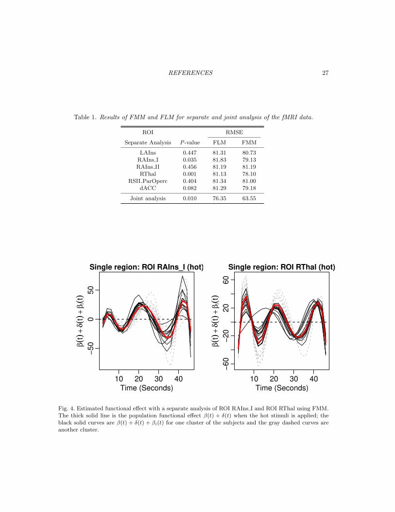
Table 1 for a list of names of these ROIs.

We first conduct a joint analysis of all 6 ROIs using the functional mixed model. The residual

plot in Figure S.4 in Section S.3 of the Supplementary Materials indicates that it is reasonable

to assume normality of the random errors. The equal-variance test of zeroness of subject-specific

functional effects gives a P -value of 0.010 (Table 1), hence favoring the proposed functional

mixed model over the standard functional linear mixed model. In addition, the in-sample root

mean squared estimation error of the responses for the functional mixed model is 63.55, much

smaller than 76.35, the estimation error for the standard functional linear model.

Figure 3 plots the estimated subject-specific functional effects β(t) + δ(t) + βi(t) when the

hot stimuli is applied. Overall the plots show highly diverse signals at the beginning of the trial,

followed by strong positive signal in the middle of the trial, and slightly weaker signal towards the

Functional mixed model for scalar on function regression 17

end of trial. The delayed peak occurring in the time period immediately following the conclusion

of the thermal stimuli (at time 18s) is consistent with the delayed nature of brain hemodynamics,

which peaks roughly 6 seconds after peak neuronal activation, and is consistent with timings of

other fMRI experiments (Lindquist and others, 2008). Notably, the secondary peak takes place

around the time of the pain reporting (38–44s), perhaps signaling a contribution of activity during

“pain recall”.

While the joint analysis and test indicate the existence of subject-specific random functional

effects when multiple ROIs are considered together, they cannot assess the existence of subject-

specific random effects for each individual ROI. Thus, we next carry out a separate analysis of

the data using each ROI as a univariate functional predictor; the results are summarized in Table

1. The residual plots in Figure S.5 in Section S.3 of the Supplementary Materials also indicate it

is reasonable to assume normality of random errors. Table 1 gives the root MSE (RMSE) of the

estimation using FLM and FMM with each ROI. For ROIs right anterior insula (RAIns I) and

right thalamus (RThal), FMM has smaller RMSE than FMM. Among the 6 ROIs, the models

with ROIs RAIns I and RThal give significant subject-specific random functional effect at the 0.05

significance level. For these two ROIs, Figure 4 displays the estimated subject-specific functional

effects β(t) + δ(t) + βi(t) when the hot stimuli is applied.

Finally, we conduct a 2-cluster analysis of the random functional effects to understand how

these effects differ. In each panel of Figure 4, the two clusters are denoted by either black solid

curves or gray dashed curves. For both ROIs, it appears that subjects mostly differ in the timing

of the delayed peak of brain hemodynamics, with one group having peaks around 22s and the

other group having a much later peak, e.g., about 24s for ROI RAIns I. In addition, for ROI

RThal, one group of subjects (gray curves) seems to have much pronounced delayed peak as well

as strong signal during the application of the stimuli; these diverse subject-specific random curves

indicate a better fit using the proposed model compared to the fixed population model.

18 W. Ma and others

6. Discussion

We proposed a functional mixed model to accommodate random functional effects of a univariate

or multivariate functional predictor for scalar on function regression, along with a significance

test of the random functional effects. Motivated by a fMRI study, we considered subject-specific

random effects to assess if the association of the fMRI data with pain rating are subject-specific.

We focused on functional data that are observed on a common grid, but the proposed model

may be extended to handle sparse functional data. Indeed, the model estimation in Section 2.3

of the marginal decomposition model for repeated functional data can be adapted, e.g., using

the FACE method for sparse functional data (Xiao and others, 2018) or for sparse multivariate

functional data (Li and others, 2018). However, the random score prediction method adopted in

the paper might not be optimal. Because of the sparsity of data, the predicted random scores

will necessarily be shrunk to zero. Thus, it remains to be seen how the proposed model and test

will perform for sparse functional data.

In the data application, we treated the fMRI data collected at multiple brain regions as

multivariate functional data. One may also treat the data as two-way functional data or matrix-

variate data as in Huang and others (2017). An interesting future research direction is to extend

the proposed functional mixed model for repeated matrix-variate data.

7. Software

Software in the form of R code, together with a sample input data set and complete documentation

is available at the Github website: https://github.com/lxiao5/fmm_sofr.

8. Supplementary Materials

Supplementary Materials containing additional simulation results and plots for the data applica-

tion are available online at http://biostatistics.oxfordjournals.org.

REFERENCES 19

Acknowledgments

We gratefully acknowledge the comments and suggestions of the Associate Editor and anonymous

referee that led to a much improved paper. Conflict of Interest: None declared.

Funding

Luo Xiao was partially supported by Grant Number R01NS091307 from National Institute of

Neurological Disorders and Stroke (NINDS) and Grant Number R56AG064803 from National

Institute on Aging (NIA) and Martin A. Lindquist was partially supported by Grant Numbers

R01EB016061 and R01EB026549 from National Institute of Health. This work represents the

opinions of the researchers and not necessarily that of the granting organizations.

References

Baey, Charlotte, Cournede, Paul-Henry and Kuhn, Estelle. (2019). Asymptotic dis-

tribution of likelihood ratio test statistics for variance components in nonlinear mixed effects

models. Computational Statistics & Data Analysis 135, 107 – 122.

Cardot, Herve, Ferraty, Frederic, Mas, Andre and Sarda, Pascal. (2003). Testing

hypotheses in the functional linear model. Scandinavian Journal of Statistics 30(1), 241–255.

Chen, Kehui, Delicado, Pedro and Muller, Hans-Georg. (2017). Modelling function-

valued stochastic processes, with applications to fertility dynamics. Journal of the Royal Sta-

tistical Society: Series B (Statistical Methodology) 79(1), 177–196.

Crainiceanu, Ciprian M and Ruppert, David. (2004). Likelihood ratio tests in linear mixed

models with one variance component. Journal of the Royal Statistical Society: Series B (Sta-

tistical Methodology) 66(1), 165–185.

20 REFERENCES

Di, Chong-Zhi, Crainiceanu, Ciprian M, Caffo, Brian S and Punjabi, Naresh M.

(2009). Multilevel functional principal component analysis. The annals of applied statis-

tics 3(1), 458.

Drikvandi, Reza, Verbeke, Geert, Khodadadi, Ahmad and Partovi Nia, Vahid. (2012,

08). Testing multiple variance components in linear mixed-effects models. Biostatistics 14(1),

144–159.

Eilers, P.H.C. and Marx, B.D. (1996). Flexible smoothing with B-splines and penalties (with

Discussion). Statist. Sci. 11, 89–121.

Gertheiss, Jan, Goldsmith, Jeff, Crainiceanu, Ciprian and Greven, Sonja. (2013).

Longitudinal scalar-on-functions regression with application to tractography data. Biostatis-

tics 14(3), 447–461.

Goldsmith, Jeff, Bobb, Jennifer, Crainiceanu, Ciprian M., Caffo, Brian and Reich,

Daniel. (2011). Penalized functional regression. Journal of Computational and Graphical

Statistics 20(4), 830–851. PMID: 22368438.

Goldsmith, Jeff, Crainiceanu, Ciprian M., Caffo, Brian and Reich, Daniel. (2012).

Longitudinal penalized functional regression for cognitive outcomes on neuronal tract measure-

ments. Journal of the Royal Statistical Society: Series C (Applied Statistics) 61(3), 453–469.

Goldsmith, Jeff, Scheipl, F, Huang, L, Wrobel, J, Gellar, J, Harezlak, J, McLean,

MW, Swihart, B, Xiao, L, Crainiceanu, C and others. (2016). Refund: Regression with

functional data. R package.

Happ, Clara and Greven, Sonja. (2018). Multivariate functional principal component anal-

ysis for data observed on different (dimensional) domains. Journal of the American Statistical

Association 113(522), 649–659.

REFERENCES 21

Huang, Lei, Reiss, Philip T., Xiao, Luo, Zipunnikov, Vadim, Lindquist, Martin A. and

Crainiceanu, Ciprian M. (2017). Two-way principal component analysis for matrix-variate

data, with an application to functional magnetic resonance imaging data. Biostatistics 18(2),

214–229.

Kong, Dehan, Staicu, Ana-Maria and Maity, Arnab. (2016). Classical testing in func-

tional linear models. Journal of Nonparametric Statistics 28(4), 813–838.

Li, Cai, Xiao, Luo and Luo, Sheng. (2018). Fast covariance estimation for multivariate sparse

functional data. Available at http://arxiv.org/abs/1812.00538.

Li, Yehua, Wang, Naisyin and Carroll, Raymond J. (2013). Selecting the number of prin-

cipal components in functional data. Journal of the American Statistical Association 108(504),

1284–1294.

Lindquist, Martin A. (2012). Functional causal mediation analysis with an application to

brain connectivity. Journal of the American Statistical Association 107(500), 1297–1309.

Lindquist, Martin A and others. (2008). The statistical analysis of fmri data. Statistical

science 23(4), 439–464.

Lindquist, Martin A, Spicer, Julie, Asllani, Iris and Wager, Tor D. (2012). Estimating

and testing variance components in a multi-level glm. Neuroimage 59(1), 490–501.

McLean, Mathew W, Hooker, Giles and Ruppert, David. (2015). Restricted likelihood

ratio tests for linearity in scalar-on-function regression. Statistics and Computing 25(5), 997–

1008.

Morris, Jeffrey S. (2015). Functional regression. Annual Review of Statistics and Its Appli-

cation 2, 321–359.

22 REFERENCES

Park, So Young and Staicu, Ana-Maria. (2015). Longitudinal functional data analysis.

Stat 4(1), 212–226.

Petrovic, Predrag, Kalso, Eija, Petersson, Karl Magnus and Ingvar, Martin.

(2002). Placebo and opioid analgesia–imaging a shared neuronal network. Science 295(5560),

1737–1740.

Qu, Long, Guennel, Tobias and Marshall, Scott L. (2013). Linear score tests for variance

components in linear mixed models and applications to genetic association studies. Biomet-

rics 69(4), 883–892.

Ramsay, James O. (2006). Functional data analysis. Wiley Online Library.

Reiss, Philip T, Goldsmith, Jeff, Shang, Han Lin and Ogden, R Todd. (2017). Methods

for scalar-on-function regression. International Statistical Review 85(2), 228–249.

Scheipl, Fabian, Greven, Sonja and Kuechenhoff, Helmut. (2008). Size and power of

tests for a zero random effect variance or polynomial regression in additive and linear mixed

models. Computational Statistics & Data Analysis 52(7), 3283–3299.

Su, Yu-Ru, Di, Chong-Zhi and Hsu, Li. (2017). Hypothesis testing in functional linear

models. Biometrics 73(2), 551–561.

Swihart, Bruce J., Goldsmith, Jeff and Crainiceanu, Ciprian M. (2014). Restricted

likelihood ratio tests for functional effects in the functional linear model. Technometrics 56(4),

483–493.

Xiao, L., Li, C., Checkley, W. and Crainiceanu, C.M. (2018). Fast covariance estimation

for sparse functional data. Statistics and Computing 28, 511–522.

Xiao, Luo, Zipunnikov, Vadim, Ruppert, David and Crainiceanu, Ciprian. (2016). Fast

REFERENCES 23

covariance estimation for high-dimensional functional data. Statistics and computing 26(1-2),

409–421.

Yao, Fang, Muller, Hans-Georg and Wang, Jane-Ling. (2005). Functional data analysis

for sparse longitudinal data. Journal of the American Statistical Association 100(470), 577–

590.

24 REFERENCES

Fig. 1. Data from the fMRI study: (a) and (c) give the fMRI time series at ROI LAIns for two subjectseach with three repetitions; (b) presents the corresponding spaghetti plots of pain ratings.

REFERENCES 25

0.00 0.05 0.10 0.15

0.0

0.2

0.4

0.6

0.8

1.0

I=20, J=20

τ2

Pow

er

curv

e

0.00 0.05 0.10 0.15

0.0

0.2

0.4

0.6

0.8

1.0

I=20, J=50

τ2

Pow

er

curv

e

0.00 0.02 0.04 0.06 0.08 0.10

0.0

0.2

0.4

0.6

0.8

1.0

I=50, J=20

τ2

Pow

er

curv

e

0.00 0.02 0.04 0.06 0.08 0.10

0.0

0.2

0.4

0.6

0.8

1.0

I=50, J=50

τ2

Pow

er

curv

e

0.00 0.01 0.02 0.03 0.04

0.0

0.2

0.4

0.6

0.8

1.0

I=200, J=20

τ2

Pow

er

curv

e

0.00 0.01 0.02 0.03 0.04

0.0

0.2

0.4

0.6

0.8

1.0

I=200, J=50

τ2

Pow

er

curv

e

Fig. 2. Power of three tests at the 5% level for the correlated functional predictor Xij(t) and as a functionof τ2. Black lines are for smooth functional data, i.e., r = 0 while gray lines are for noisy functional data.Solid lines: equal-variance test; dashed lines: Bonferroni-corrected test; dot-dashed lines: asLRT.

26 REFERENCES

−40

−20

020

40

Multiple regions: ROI LAIns (hot)

Time (Seconds)

β(t

)+

δ(t

)+β

i(t)

10 20 30 40

−5

00

50

Multiple regions: ROI RAIns_I (hot)

Time (Seconds)β(t

)+

δ(t

)+β

i(t)

10 20 30 40

−4

0−

20

020

40

Multiple regions: ROI RAIns_II (hot)

Time (Seconds)

β(t

)+

δ(t

)+β

i(t)

10 20 30 40

−40

−2

00

20

40

60

Multiple regions: ROI RThal (hot)

Time (Seconds)

β(t

)+

δ(t

)+β

i(t)

10 20 30 40

−4

0−

20

020

40

Multiple regions: ROI RSII_ParOperc (hot)

Time (Seconds)

β(t

)+

δ(t

)+β

i(t)

10 20 30 40

−40

−20

020

40

Multiple regions: ROI dACC (hot)

Time (Seconds)

β(t

)+

δ(t

)+β

i(t)

10 20 30 40

Fig. 3. Estimated functional effect with a joint analysis of 6 ROIs using FMM. The black solid line is thepopulation functional effect β(t) + δ(t) when the hot stimuli is applied; the gray dashed curves are thesubject-specific random functional effect β(t) + δ(t) + βi(t).

REFERENCES 27

Table 1. Results of FMM and FLM for separate and joint analysis of the fMRI data.

ROI RMSE

Separate Analysis P-value FLM FMM

LAIns 0.447 81.31 80.73RAIns I 0.035 81.83 79.13RAIns II 0.456 81.19 81.19

RThal 0.001 81.13 78.10RSII ParOperc 0.404 81.34 81.00

dACC 0.082 81.29 79.18

Joint analysis 0.010 76.35 63.55

−50

050

Single region: ROI RAIns_I (hot)

Time (Seconds)

β(t

)+

δ(t

)+

βi(t

)

10 20 30 40

−60

−20

20

60

Single region: ROI RThal (hot)

Time (Seconds)

β(t

)+

δ(t

)+

βi(t

)

10 20 30 40

Fig. 4. Estimated functional effect with a separate analysis of ROI RAIns I and ROI RThal using FMM.The thick solid line is the population functional effect β(t) + δ(t) when the hot stimuli is applied; theblack solid curves are β(t) + δ(t) + βi(t) for one cluster of the subjects and the gray dashed curves areanother cluster.