A Generalized Radiosity Simulation Model and Full-Scale ...

A Generalized Radiosity Simulation Model and Full-Scale Experimental Verification of a Corner Office having Three Section Façade with Motorized Shading

Shahriar Hossain

A Thesis

In

The Department

of

Building, Civil and Environmental Engineering

Presented in Partial Fulfillment of the Requirements

for the Degree of Master of Applied Science (Building Engineering) at

Concordia University

Montreal, Quebec, Canada

September 2016

© Shahriar Hossain, 2016

ii

CONCORDIA UNIVERSITY

School of Graduate Studies

This is to certify that the thesis prepared

By: Shahriar Hossain

Entitled: A Generalized Radiosity Simulation Model and Full-Scale Experimental Verification of a Corner Office having Three Section Façade with Motorized Shading

and submitted in partial fulfillment of the requirement for the degree of

Master of Applied Science (Building Engineering)

complies with the regulations of the University and meets the accepted standards with respect to originality and quality.

Signed by the final Examining Committee:

Dr. Hua Ge Chair

Dr. Ahmed Kishk External Examiner

Dr. Fuzhan Nasiri Examiner

Dr. Andreas Athienitis Supervisor

Approved by _______________________________________________________

Chair of Department or Graduate Program Director

_______________________________________________________

Dean of Faculty

Date _______________________________________________________

iii

Abstract

A Generalized Radiosity Simulation Model and Full-Scale Experimental Verification of a Corner Office having Three Section Façade with Motorized Shading

Shahriar Hossain

Daylight distribution models are essential for daylighting design and present information in a visual

manner that facilitates decision making. With an accurate model, daylight in a space can be

distributed in an efficient and comfortable way, so that the need for electric lighting in daytime is

reduced. On the other hand, motorized shades can be controlled automatically to better distribute

daylight on the work plane and reduce or avoid glare.

Most of modern buildings, both commercial and high-rise residential, have windows in more than

one orientation and have the provision for daylight penetration into space. In this study, a radiosity

model for simulating the daylight distribution of a corner office having two windows in various

orientations with motorized shades has been developed. The model calculates the illuminance at

different locations on the work plane.

The simulation model based on radiosity theory is verified with measured data under overcast and

clear sky conditions with direct and diffuse lighting, and a parametric analysis is carried out for

various room shapes and shading devices and façade orientations. The model is implemented in

Mathcad and used to predict the illuminance distribution in the room for developing improved

control strategies for shade positions and also for design guidelines to select the properties of the

shades. Three section façade is considered with the bottom section being opaque (spandrel), the

middle viewing section and a top daylighting section. Variable shade transmittance in the middle

iv

and top section of the facades is studied, and it is shown that having a higher transmittance in the

top section results in improved daylight utilization and a middle section with lower transmittance

provide privacy to the building occupants. Specific recommendations are made for shade

transmittances for upper and middle part of the façade to maintain occupant privacy with acceptable

illuminance in the work-plane.

v

Acknowledgments

Firstly, I sincerely thank my supervisors Dr. Andreas K. Athienitis for his guidance, suggestion, and

belief on me. This thesis is the result of his kind assistance, motivation, and encouragement.

Thanks to my colleagues in the Solar Lab for their continuous support and assistance, specially to

Dr. Konstantinos Kapsis and Dr. Jiwu Rao for their suggestions and helpful advice.

I would also like to thank my relatives and friends in Montreal from Bangladesh, who made this

lonely place livable for me.

I am forever grateful to my parents and my lovely wife. Without their sacrifice and support, I couldn’t

be able to make this real. I’m all about, only because of them.

I acknowledge the financial support of the Natural Sciences and Engineering Research Council of

Canada (NSERC) through a NSERC/ Hydro-Québec Industrial Chair and the industrial partners –

Hydro-Québec and Regulvar.

vi

Table of Contents

List of Figures……………………………………………………………………………………………………………………..ix

Nomenclature…………………………………………………………………………………………………………………….xii

Chapter 1: Introduction ................................................................................................................... 1

1.1 Background ............................................................................................................................ 1

1.2 Motivation .............................................................................................................................. 2

1.3 Objectives ............................................................................................................................... 3

1.4 Corner room with 3 section façade on each side ................................................................. 4

1.5 Thesis Overview ..................................................................................................................... 5

Chapter 2: Literature Review ............................................................................................................ 6

2.1 Introduction ........................................................................................................................... 6

2.2 Sunlight on Earth ................................................................................................................... 6

2.3 Daylight modeling approaches .............................................................................................. 7

2.4 Different types of Shading ................................................................................................... 11

2.5 Shade control strategies ....................................................................................................... 12

2.6 Occupant comfort and privacy ............................................................................................ 15

2.7 Conclusion ........................................................................................................................... 16

Chapter 3: Radiosity Model of the Corner Room ......................................................................... 18

3.1 Introduction ......................................................................................................................... 18

3.2 Solar Position and Angles .................................................................................................... 19

3.3 Sky model ............................................................................................................................. 21

3.3.1 CIE Overcast Sky .......................................................................................................... 22

vii

3.3.2 CIE Clear Sky ............................................................................................................... 22

3.3.3 Perez all-weather sky model .......................................................................................... 23

3.4 Radiosity Method ................................................................................................................. 23

3.5 Model Description ............................................................................................................... 25

3.6 Daylight Glare Probability (DGP) ....................................................................................... 30

Chapter 4: Experiment and model Verification ............................................................................ 32

4.1 Introduction ......................................................................................................................... 32

4.2 Properties of the room components .................................................................................... 33

4.3 Experimental set-up .............................................................................................................. 33

4.3.1 Li-Cor Photometer ....................................................................................................... 34

4.3.2 Data Acquisition System .............................................................................................. 35

4.3.3 Façade ........................................................................................................................... 35

4.3.4 Shades ........................................................................................................................... 35

4.4 Sensor positioning ............................................................................................................... 36

4.5 Experimental verification on overcast day .......................................................................... 37

4.6 Parametric Analysis .............................................................................................................. 42

Chapter 5: Conclusion ................................................................................................................... 53

5.1 Conclusions .......................................................................................................................... 53

5.2 Future Work ......................................................................................................................... 55

References ............................................................................................................................................ 56

Appendix A.......................................................................................................................................... 60

Appendix B .......................................................................................................................................... 61

Appendix C ......................................................................................................................................... 62

viii

Appendix D ......................................................................................................................................... 63

ix

List of Figures:

Figure 1: A three Section facade concept (Kapsis and Athienitis 2015) ............................................. 2

Figure 2: A typical three section façade having windows in two orientations .................................... 4

Figure 3: Visible Spectrum (Murdoch 2003) ........................................................................................ 7

Figure 4: Comparison of illuminance level between 3-surface, 7-surface and complex 600-surface

model (Athienitis and Boxer 2011) ...................................................................................................... 9

Figure 5: Hybrid ray tracing and radiosity method flowchart (Chan and Tzempelikos 2012) ......... 10

Figure 6: Glare free zone concept (Kapsis et al. 2010) ....................................................................... 11

Figure 7: Possible classification of shading (Bellia et al. 2014) .......................................................... 12

Figure 8: Closed-loop control strategies for lighting (Mukherjee et al. 2010) ................................... 13

Figure 9: Shade control integrated with electric lighting (Shen et al. 2014) ..................................... 14

Figure 10: Influence of lighting on human performance (Boyce et al. 2003) ................................... 15

Figure 11: Blind position vs solar penetration depth for irradiance over and below 50 W/m2

(Reinhart and Voss 2003) ................................................................................................................... 16

Figure 12: Solar geometry (Athienitis 1999) ...................................................................................... 20

Figure 13: A 14-Surface Room Enclosure for view factor calculation ............................................... 25

Figure 14: Illuminance on an overcast day (June 9, 2015) ................................................................ 26

Figure 15: Top view of the workplane showing the five by five array simulation points

(measurement points are circled) ........................................................................................................ 27

Figure 16: Shading position configurations ....................................................................................... 30

Figure 17: Engineering and visual Arts (EV) building, Concordia University, Montreal, QC

(www.concordia.ca).............................................................................................................................. 32

x

Figure 18: Experiment Set-ups in a full-scale office room .................................................................. 34

Figure 19: Li-cor LI-210 Photometric sensor ...................................................................................... 35

Figure 20: Schematic of the sensor position on the work plane. ...................................................... 36

Figure 21: Schematic of the sensor position on the windows ........................................................... 37

Figure 22: Selected points of measurement on the work plane ........................................................ 38

Figure 23: Measured vs simulated data of illuminance on work-plane (lux) ..................................... 39

Figure 24: Illuminance comparison for all open shade configuration .............................................. 40

Figure 25: Illuminance comparison for 25% shade configuration.................................................... 40



Figure 28: Illuminance comparison for all closed shade configuration ............................................ 42

Figure 29: Work plane illuminance vs floor reflectance (for all shades open) .................................. 43

Figure 30: Work plane illuminance vs floor reflectance (for all shades closed) ................................ 44

Figure 31: Work plane illuminance vs shade transmittance ............................................................. 44

Figure 32: Work-plane illuminance due to different shade transmittance on different sections of

near-south and near-east facades. ........................................................................................................ 46


near-east façade (Considering near-south facade is opaque). ............................................................. 47


near-south façade (Considering near-east facade is opaque). ............................................................. 48

Figure 35: Calculated Daylight Glare Probability (DGP) for different shade transmittances on

different sections of both façades. ...................................................................................................... 50

xi


different sections of near-east façade (Considering near-south facade is opaque). ........................... 51


different sections of near-south façade (Considering near-east facade is opaque). ........................... 52

xii

Nomenclature

W1 Room length (m)

W2 Room width (m)

H Room Height (m)

Y1 Spandrel height (m)

Y2 Height of the clear glass section (m)

Y3 Height of the fritted glass section (m)

M Luminous exitance (lx)

Fij View factor from surface i to j

τ Visible transmittance

ρ Visible reflectance

Lz Sky luminance at zenith.

Eho Horizontal illuminance (lx)

Evo Vertical Illuminance (lx)

Ext Extraterritorial solar radiation (W/m2)

Esc Solar illuminance constant (lx)

Edn Solar illuminance at sea level (lx)

J Julian day number

α Solar altitude

𝛿 Solar Declination Angle

φ Solar azimuth

γ Surface solar azimuth

xiii

d Profile angle

θ Angle of incidence

V Spectral Luminous Efficiency

𝜆 Wevelength

k Maximum luminous efficacy

E Illuminance (lx)

N Total number of surfaces

C Configuration factor

z, y, w Distance of enclosed surfaces from point of interest

Subscripts

i, j Index

0 Initial value

point Point of interest

1

Chapter 1: Introduction

1.1 Background

The use of energy is increasing with continuously as it is an essential element in our lives.

Saving energy and the environmental impacts of energy production and use are a major

concern worldwide. According to Energy use data handbook, 1990-2013 (Natural Resource

Canada) , lighting energy is 12% of the total energy used in commercial buildings in Canada.

As commercial buildings have larger facades with transparent or colored glass, study of daylight

has become a primary choice for researchers. Daylighting plays a major role in occupant

comfort and behavior and as has a direct impact on energy use. Daylight, that is visible solar

radiation, which is about 42% of total solar radiation, has an immediate impact on human

health and performance. Research shows that students, having a classroom with more window

area score 7% to 18% higher on a standardized than others (Heschong et al. 2002). However,

daylighting system should be designed carefully, as they can be a cause for overheating of the

space or discomfort due to glare.

In order to control the penetration of sunlight into the space, an optimized and accepted

daylight model should be developed. There are different types of models and simulation

software are present, which simulates the daylight distribution through windows on a certain

orientation. Windows in more than one façade is a different scenario than in one. Almost

every building has such location at corner perimeter of the building. A better design of that

type of corner office or zone of the building can increase occupant performance and reduces

the energy consumption for lighting and HVAC system. In addition, motorized shading

2

systems can be optimally operated and positioned based on daylight levels, occupancy of the

space and the need to prevent glare.

1.2 Motivation

Modeling of a corner room with façade on near-south and near-east side utilizing the three-

section façade design concept is a new field of research to study the corner perimeter zone of

a building. The three section façade (Kapsis et al. 2015) consists of a lower part of the opaque

(spandrel) panel, a middle section of clear glazing and an upper section of fritted glass. The

top can be used to distribute daylight to the deeper parts of the room without the need of full

view to the outdoors; architects often use fritted glass to reduce solar gains while allowing

much daylight through but a better option would be to use semitransparent photovoltaic

glazing in place of fritted glass to allow daylight transmission but also generate solar electricity.

Figure 1: A three Section facade concept (Kapsis and Athienitis 2015)

3

Daylight mathematical models calculate interior light levels in space and on the work plane

which is generally assumed to be a virtual horizontal surface about 0.8 m above the floor.

Models use different sky scenarios, such as clear sky or overcast, or real world weather data

files for a particular location. A building can be tested early in the design phase by simulating

with the model or existing buildings can be studied as part of a retrofit strategy to select new

shading devices, new lighting systems or a new control system that can dim the lights in order

to save energy by using more daylight. There are many software packages available for general

simulation, but the primary purpose of the model described in this thesis to be used to develop

a shade control strategy with a bottom-up approach to prevent glare and maintain acceptable

light levels on the workplane.

For that purpose, the radiosity method (Athienitis and Tzempelikos 2002) is used to simulate

the office and compare with measured data to validate the model and simulate different

configurations of shade and interior surfaces. The model is general so that it can be used with

fenestration on just one façade by changing the properties of the interior surfaces.

1.3 Objectives

The primary objectives of this thesis are as below

To develop a radiosity model to analyze the daylight distribution of a corner office with

windows on two sides.

To see the effect of the different position of motorized shades on a three section façade.

To validate the developed model through an experimental result in a full scale office.

4

To investigate different design options by varying properties of the interior surface and

glazing properties and to develop design guidelines.

1.4 Corner room with 3 section façade on each side

Most commercial buildings nowadays have larger façade with glass all around it. Those

perimeter zone of the buildings have the provision for daylight penetration through windows

made of glass. Almost all of those buildings have corner portion with a window in more than

one orientation.

In this thesis, a similar kind of room is studied, which has windows on near south and near

west direction. Each of those three section façades is formed with the bottom section being

opaque (spandrel), the middle viewing section with clear glass and a top daylighting section

with fritted glass. Figure 2 shows a typical three section façade having windows in two

directions

Figure 2: A typical three section façade having windows in two orientations

5

1.5 Thesis Overview

Chapter 2 presents a literature review of recent and past work done by researchers in this field.

These reviews consist of daylight and studies various modeling approaches, different types of

shading devices, shade control strategies, glare prevention techniques, and occupant behavior,

comfort, and privacy.

Chapter 3 describes the detailed radiosity model of a corner office room with windows on two

adjacent façades. A fourteen-surface room enclosure model was considered (Two vertical walls,

floor, ceiling, and three sections of each façade divided into two part for shading position

calculation) for the calculations of view factors needed in the radiosity model. Initial luminous

exitance was calculated using CIE overcast sky model. Then the configuration factor for any

point on the workplane with respect to each interior surface was calculated and multiplied

with the final luminous exitance to get the workplane illuminance.

Chapter 4 validates the model with experimental data. The detail explanation of the

experiment and the equipment used are discussed in this section. A parametric analysis for

various shade transmittances and floor reflectance were performed.

Chapter 5 presents the conclusions of the thesis and recommendations for future possibilities

of this work.

6

Chapter 2: Literature Review

2.1 Introduction

Modern buildings are becoming more stylish and their peremeter zones are becoming more

transparent. This approach of newly built building reduces the thermal mass and thus increase

the energy uses. To improve the performace of the building in terms of energy uses façade

design approaches has been the primary concern for the engineers. This chapter of the thesis

focuses on some important works done previously by other researchers. This literature review

includes daylight performance analysis of commercial buildings, shading of the fenestration,

occupancy privacy in the work area and some glare prevention strategies. This thesis describes

the daylight model for a corner office with façade on two sides. There aren’t many previous

works on this type of case.

This chapter will also include some important reviews on daylight performance indicators and

effects of different types of shading devices for offices.

2.2 Sunlight on Earth

Life exists on earth only because of the sun. The sun is the main source of light and heat on

the earth and most importantly it is free. Many researchers have done and are still doing an

extensive investigation of different ways of utilizing the power of the sun. The power of the

sun can either be used as a light source or as a heat source. These lights in heat sources are

now converted to renewable energy.

The diameter of the sun is approximately 1.39*106 KM and it is nearly 149.6 million Km away

from the earth. it mostly consists of hydrogen gas. Sunlight is only the part of the

7

electromagnetic radiation emitted my sun. Before sunlight falls on the earth surface, it crosses

the atmosphere where most of the radiation is absorbed. The earth only receives only a part

of 109 of the total energy of the sun. Before hitting the atmosphere, the solar radiation is close

to a black body and the temperature is about 5800K. From the total range of the solar

spectrum, our interest is in the visible part of that. The human eye can be responsive to the

only 380nm to 780nm wavelength of the spectrum (Murdoch 2003).

Figure 3: Visible Spectrum (Murdoch 2003)

The total extraterritorial solar radiation (Murdoch, 2003) can be expressed as

𝐸𝑥𝑡 = 𝐸𝑠𝑐 [1 + 0.034 𝑐𝑜𝑠360

365(𝑗 − 2)] (1)

2.3 Daylight modeling approaches

Sunlight has been the primary source of lighting for many years. Quantification and different

quality measures of daylight make it easy for researchers to utilize daylight more efficiently and

effectively in buildings.

For effective and efficient utilization, a model needs to be developed to characterize the

fenestration systems, including shading. There are three types of modeling techniques.

Radiosity (Applied for diffuse light)

Ray Tracing (Applied for direct light)

Hybrid (combination of both)

8

Radiosity method (Athienitis and Tzempelikos 2002) is one of them commonly used and the

illuminance at any point in a space can be predicted and the shades can be controlled

according to that prediction. Previously this method was only used to calculate the heat

transfer between surfaces. But now a day it is widely used for lighting rendering.

(Lehar and Glicksman 2007) shows this radiosity method as a rapid algorithm for lighting

analysis. The main part of the calculation is to determine the view factor. If the view factor is

calculated once the lighting calculation can be done easily by varying other parameters. They

used the radiosity method for the diffuse light calculation and then added the direct sunlight

contribution through the window with it. They found approximately 10% error compared to

the verified lighting simulation software to their calculation and accepted that variation.

On the other hand, (Athienitis and Boxer 2011) showed a comparison between simple

radiosity method (3 surfaces and 7 surfaces) and a detailed 600 surface radiosity model and

found that the 7 surface model gives very close result as of the 600 surface.

9

Figure 4: Comparison of illuminance level between 3-surface, 7-surface and complex 600-surface model (Athienitis and Boxer 2011)

The direct sunlight that enters the room through the unshaded part of the window can be

calculated by the ray-tracing method (Kuhn et al. 2001). This method traces the path of sun

rays and shows the sun patch on the room (Glassner 1989). This method is ideal for analyzing

daylight distribution where direct light is important and glare prevention is a must. It indicates

the pattern of the beam and direct glare so that the shade can be controlled accordingly (Kapsis

et al. 2010). This method is also important to the designer of venetian blinds (Tzempelikos et

al. 2007).

(Chan and Tzempelikos 2012) also presented a hybrid ray tracing and radiosity method to

calculate the daylight distribution more accurately.

10

Figure 5: Hybrid ray tracing and radiosity method flowchart (Chan and Tzempelikos 2012)

Direct glare prevention was also partly done with bottom-up roller shades (Kapsis et al. 2010)

and analyzed using the ray-tracing method. They described a glare free zone (GFZ) and traced

the sun ray path to determine that zone.

11

Figure 6: Glare free zone concept (Kapsis et al. 2010)

2.4 Different types of Shading

With the increased use of fenestration in façades, it is essential to design shading and

daylighting systems together with appropriate strategies for their control so that daylight is

used effectively while preventing glare.

Research into different types of shades and blinds such as venetian blinds, (Tzempelikos et al.

2007), (Mettanant and Chaiwiwatworakul 2014), (Lee et al. 1998), bottom up shades (Kapsis

et al. 2010) is also ongoing. Dynamic window technologies have been studied recently, where

shades can be located internally, externally or in-between the window panel as a possible

classification of shading proposed by (Bellia et al. 2014).

12

Figure 7: Possible classification of shading (Bellia et al. 2014)

External shades have stronger effect on the heating and daylight than internal shading (Morini

et al. 2014). But interior shades are most common in commercial buildings in Canada as they

can be installed after the initial design stage without affecting the exterior appearance of the

building and they have low maintenance and are easy to install. In addition they are not

affected by exterior snow and freezing rain. With the bottom-up shades it is reported that 8-

58% higher daylight autonomy can be obtained compared to conventional roller shades which

operate from top to bottom. This type of shade contributes to saving energy for the artificial

lighting of 21-41% (Kapsis et al. 2010).

2.5 Shade control strategies

Roller shades are one of the most common, efficient and easiest ways to control the amount

of light entering a space. Using shades on windows, the direct sunlight and the solar heat gain

can be controlled and the energy consumption can be reduced (Mills and McCluney 1993);

(Athienitis and Santamouris 2002). Shades can be positioned manually, but controlling the

position of motorized shades automatically can be more efficient and cost-effective in terms of

energy consumption (Kapsis et al. 2010) and glare minimization.

13

Shade control strategies can be open-loop or closed-loop. Open loop control system of blinds

involves a model and the pre-calculated solar angles to determine the position of the shades

accordingly (Skelly and Wilkinson 2001), (Vine et al. 1998), (Shen and Tzempelikos 2014).

On the other hand closed-loop control strategies need the sensor value to be fed backed to the

system (Reinhart and Voss 2003), (Mukherjee et al. 2010).

Figure 8: Closed-loop control strategies for lighting (Mukherjee et al. 2010)

(Shen et al. 2014) examined and compared three types of control with seven different strategies

(Table-1). In the manual control strategy (1), the lights are controlled by on (with or without

dimming) or off position as per occupant’s presence. The first five independent control

strategies daylight and lighting control work independently, whereas in the last two integrated

strategies daylight and lighting are being controlled by sharing the control information with

HVAC system.

14

Table: 1: Types of control with different strategies.

Control type Control strategy

Manual control

Strategy 1: Manual control of lights and no blinds

Independent control

Strategy 2: Independent open-loop blind, closed-loop dimming control Strategy 3: Independent open-loop blind, closed-loop dimming control, occupancy and HVAC mode shared with blind system Strategy 4: Independent closed-loop blind, closed-loop dimming control Strategy 5: Independent closed-loop blind, closed-loop dimming, occupancy and HVAC mode shared with blind system

Integrated control

Strategy 6: Fully integrated lighting and daylighting control with blind tilt angle control without blind height control Strategy 7: Fully integrated lighting and daylight control with blind tilt angle and height control

They showed a fully integrated open-loop and closed-loop lighting and daylighting control

system in accordance with the sun angle, HVAC sensor, photo sensor and occupancy sensor.

Figure 9: Shade control integrated with electric lighting (Shen et al. 2014)

15

2.6 Occupant comfort and privacy

Daylight utilization in perimeter zones of office buildings is particularly important as it reduces

the need for electric lighting and it contributes to a higher quality indoor environment (Boyce

et al. 2003); (Farley and Veitch 2001). Boyce has given a conceptual chart which shows the

impact of lighting condition in a room on the occupant’s visual performance.

Figure 10: Influence of lighting on human performance (Boyce et al. 2003)

16

Presently, many researchers are working on modeling daylight in buildings and controlling it

according to occupant needs (Muller et al. 1995); (Robinson and Stone 2006).

A real life study (Reinhart and Voss 2003) shows that people in the office close their shades

when the direct sunlight is over 50 W/m2 on the work plane.

Figure 11: Blind position vs solar penetration depth for irradiance over and below 50 W/m2 (Reinhart and Voss 2003)

When it comes to venetian blinds many people keep the blinds down with the slats in the

horizontal position either for privacy or they like to use the artificial lights rather than moving

the blinds manually (Escuyer and Fontoynont 2001).

2.7 Conclusion

A lot of effort has been made by researchers for modeling daylight penetration in space. Models

consist of various aspect on energy saving, glare prevention and light levels control strategies.

Some models are integrated with the building HVAC system to develop control strategies to

reduce solar heat gain.

17

Based on the literature review, it can be concluded that continued research is needed to save

energy by using more daylight rather than electric lighting while preventing glare. This needs to

be done both the design stage of a building by selecting appropriate shading and daylighting

systems and developing improved methods for their control.

This thesis works on both of the above needs for the specific configuration of a corner office

that has windows on two orientations.

18

Chapter 3: Radiosity Model of the Corner Room

3.1 Introduction

A corner room in a commercial building is most demandable because it has windows on two

adjacent façade compared to the most common case of having only one window or no window.

Corner rooms have more exposure to the sunlight than other rooms in the buildings. Though

the area ratio of the corner space to the other conventional spaces in the perimeter zone of a

building is not significant, it is more important to analyze and design carefully. Because of

having glass façade on two sides, these areas can be over heated or can face more glare from

the sunlight.

This model describes the most common case of an office perimeter corner zone (figure-2). By

varying the non-dimensionalized room dimensions (such as 𝑊1

𝑊2,

𝑊1

𝐻,

𝑊2

𝐻 ), façade aspect ratio

(such as 𝑌1

𝐻,

𝑌2

𝐻,

𝑌3

𝐻) or surface properties, the daylight distribution of any space with

fenestration at any orientation can be simulated and analyzed. This model consists of a three

section façade where the lower part is opaque (spandrel), the middle section is clear and the

upper section is fritted glass.

To develop this model, the radiosity method was used to predict the daylight distribution at

different points of interest in an office. The radiosity method is based on diffuse daylight

transmitted through the windows/shades and the daylight reflected from the interior surfaces

also assumed to be diffuse. This model was developed by using the Mathcad 15 program.

Some assumptions were made to develop the model. Those are:

19

All internal surfaces of the room are diffuse.

There are no external obstacles.

The reflectance of the room surfaces is calculated as an area weighted average.

The input parameters of the model are as below:

The geographic location,

The room dimensions,

The reflectance of the interior surfaces, glazing and shades,

The visible transmittance of the glazing and shades, and

The sky condition.

3.2 Solar Position and Angles

To analyze the daylight, it is very important to know the relationship of earth to the sun. To

calculate the exact position of the sun some angles are used. The definitions and schematic of

those solar angles are described below.

20

Figure 12: Solar geometry (Athienitis 1999)

Solar Declination Angle (δ)

Solar declination angle is the angle between the earth-sun line and the equatorial plane on

a specific day.

𝛿(𝑛) = 23.45 × sin (360 ×284+𝑛

365) (2)

Where n is the number of the day of the year. i.e. n=1 for January 1.

Solar altitude (αs)

The altitude angle is the angle between the sun rays and the horizontal plane on earth. This

angle often describes how high the sun appears in the sky.

sin 𝛼𝑠 = 𝑠𝑖𝑛𝐿. 𝑠𝑖𝑛𝛿 + 𝑐𝑜𝑠𝐿. 𝑐𝑜𝑠𝛿. 𝑐𝑜𝑠𝐻 (3)

Where L= latitude of the location and H=Hour Angle

21

The altitude angle is negative when the sun drops below the horizon.

Solar azimuth (φ)

Solar azimuth is the angle between the projected sun rays on a horizontal plane from the

due south. The angle is measured positive eastward.

𝑠𝑖𝑛𝜑 = 𝑐𝑜𝑠𝛿.𝑠𝑖𝑛𝐻

𝑐𝑜𝑠𝛼𝑠 (4)

Surface solar azimuth (γ)

This is the angle between the projection of the sun rays to the horizontal plane and the line

normal to the surface.

Angle of incidence (θ)

This is the angle between the sun rays and normal to the surface.

Profile angle (d)

Profile angle is the vertical angle from the horizon of the sun projected onto the horizontal

plane.

3.3 Sky model

The international commission on illumination (CIE) published a standard sky model for the

overcast and clear sky in 1996, and this model is accepted worldwide for luminance

distribution and daylighting analysis. This model defines the luminance of the sky at any point

and calculates the illuminance at any surface on earth.

A more detail mathematical sky model developed by (Perez et al. 1990) is also known as Perez

All-Weather sky Model. Real weather data are used as an input of this model.

22

3.3.1 CIE Overcast Sky

The overcast sky is described where clouds completely cover the sky, and the sun is not

visible. This is the condition where the sunlight is completely diffused by the clouds.

Based on the CIE overcast sky model, the horizontal illuminance at any point (Murdoch,

2003) is defined by

𝐸ℎ𝑜 = 300 + 21000𝑠𝑖𝑛𝛼𝑠 (lx) (5)

The vertical illuminance due to the diffused light is 40% of the horizontal illuminance.

𝐸𝑣𝑜 = 0.4𝐸ℎ𝑜 (lx) (6)

3.3.2 CIE Clear Sky

For clear sky modeling, the sky luminance depends on various angles. Under this condition,

beam (direct solar radiation) is excluded and again light from the clear sky is diffuse. Firstly

the average illuminance on a surface perpendicular to the sun rays and just at the outer

atmosphere can be calculated by

𝐸𝑠𝑐 = 𝑘 ∫ 𝐸𝑠𝜆𝑉(𝜆)𝑑𝜆0.78

0.38= 127.5 𝐾𝑙𝑥 (7)

Where, V(𝜆) is the spectral luminous efficiency of the eyes, k is the maximum luminous

efficacy (683lm/W). This Esc is called the solar illuminance constant.

The actual illuminance on any day of the year outside the earth atmosphere on a surface

perpendicular to the sun rays is as follow

𝐸𝑥𝑡 = 𝐸𝑠𝑐 [1 + 0.034 cos360

365(𝑛 − 2)] (8)

23

Where, n is the number of the day in a year.

The solar illuminance to the sea level (Edn) can be expressed as

𝐸𝑑𝑛 = 𝐸𝑥𝑡. 𝑒−𝑐𝑚 (9)

Where c is the optical atmospheric extinction coefficient with a value for clear sky of 0.21

and m is the relative optical mass. m can be expressed in terms of solar altitude as

𝑚 =1

𝑠𝑖𝑛𝛼𝑠

Now the horizontal illuminance on a given surface is given by

𝐸ℎ𝑑 = 𝐸𝑑𝑛. 𝑠𝑖𝑛𝛼𝑠 (10)

3.3.3 Perez all-weather sky model

This model is used to explain the relative luminance distribution of the sky depending on

two key parameters, the sky brightness and the sky clearness. These two parameters can be

calculated from the diffuse horizontal and direct normal irradiance data for specific location

and time.

This model gives a realistic sky illuminance data calculated from the different atmospheric

condition, which are used for daylight calculations.

3.4 Radiosity Method

The radiosity method is based on diffuse daylight transmitted through the windows/shades

and the daylight reflected from the interior surfaces. Initially, this method was only used to

solve the radiation heat transfer equations. The amount of light radiated from a surface is the

24

summation of the initial luminous exitance of that surface and the amount of reflected light

from that surface.

𝑀𝑖 = 𝑀0𝑖 + 𝜌𝑖 ∑ 𝑀𝑗𝐹𝑖,𝑗𝑗 (11)

where,

Mi = Final luminous exitance of surface i (lx)

M0,i = Initial luminous exitance of surface i (lx)

ρi = Reflectance of surface i

Mj = Final luminous exitance of surface j (lx)

Fi,j = View factor between surfaces i and j

Radiosity is a method to compute the amount of light between different diffused surfaces in

an enclosure. There are some steps to follow for solving a radiosity problem

Calculate the initial luminous exitance of each surface enclosure, if any.

Calculate the effective reflectance of each enclosure surface.

Calculate the view factors between enclosure surfaces.

Calculate the total luminous exitance of each enclosure surface, using the radiosity

matrix.

𝑀𝑖 = 𝑀0𝑖 + 𝜌𝑖 ∑ 𝑀𝑗𝐹𝑖,𝑗𝑗 (12)

Calculate the total illuminance on a point of interest, using the configuration factors

between the enclosure surfaces and the point of interest.

7

1int,int

iipoipo McE (13)

25

3.5 Model Description

Generally, we can develop a detailed model by subdividing room surfaces into smaller discrete

regions. A fourteen-surface room enclosure (Figure 13) was considered (Two vertical walls,

floor, ceiling, and three sections of each façade divided into two parts for shading position

calculation) for the calculations. The main input parameters for this model are i) the

geographic location, ii) the room dimension, iii) the reflectance of the interior surfaces, glazing

and shades, iv) the visible transmittance of the glazing and shades, and v) the sky condition.

Figure 13: A 14-Surface Room Enclosure for view factor calculation

To find the final luminous exitance, the initial luminous exitance of each surface and the view

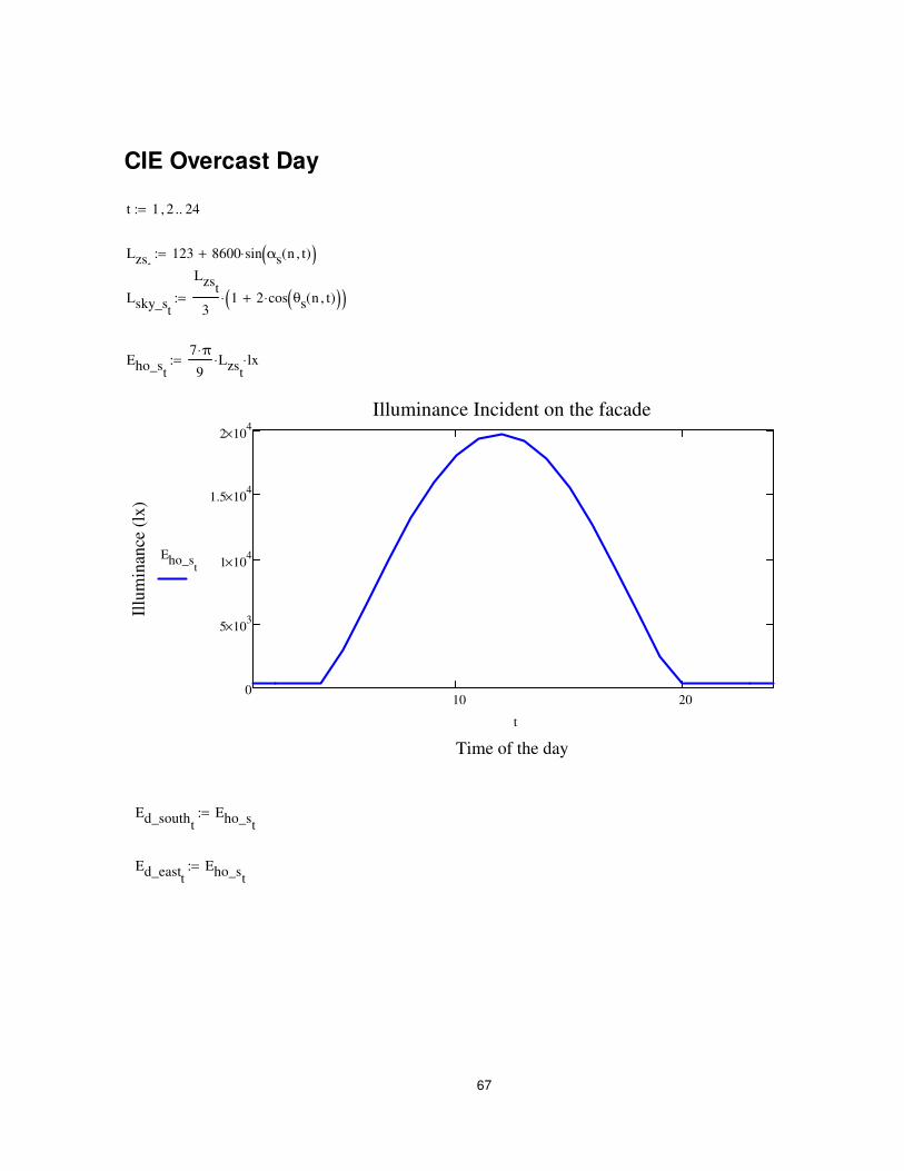
factors between room surfaces were calculated. The CIE overcast sky model was used to

calculate the initial luminous exitance. The model input is hourly diffuse irradiance, and it is

26

better suited for overcast weather conditions. Using this sky model we can estimate the

illuminance value to use in the model (Murdoch, B. 2003).

𝐿𝑧 = 123 + 8600 sin𝛼𝑡 (14)

Where, Lz is the sky luminance at zenith.

The horizontal illuminance due to overcast sky is given by (Murdoch, B. 2003),

𝐸ℎ𝑜𝑡=

7𝜋

9𝐿𝑧 = 0.30 + 21𝑠𝑖𝑛𝛼𝑡 (15)

For a day (June 9, 2015) with an overcast sky, the incident illuminance on the façade is shown

in figure 14.

Figure 14: Illuminance on an overcast day (June 9, 2015)

After calculating the total luminous exitance (Mi) of surface i, the illuminance on the point

of interest was calculated by multiplying the total luminous exitance with the configuration

factor between surface i and the point of interest

27

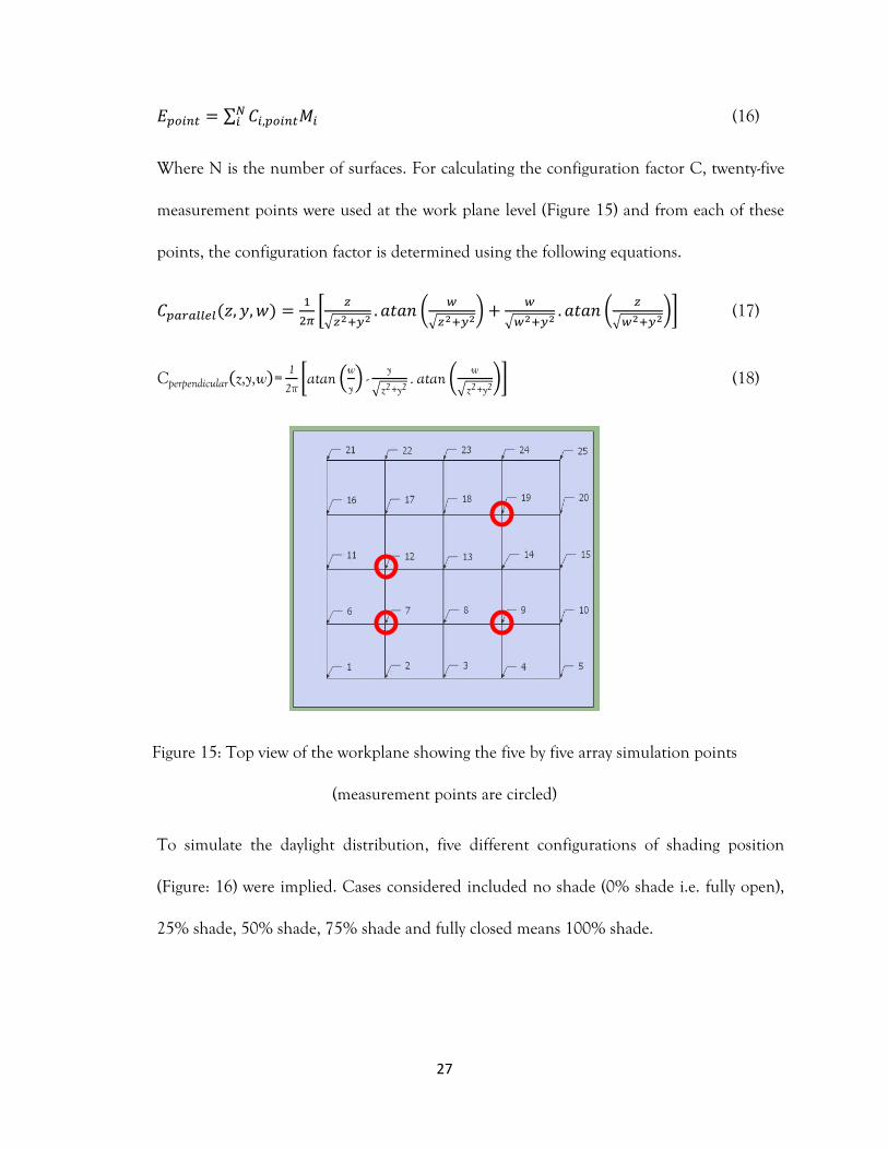
𝐸𝑝𝑜𝑖𝑛𝑡 = ∑ 𝐶𝑖,𝑝𝑜𝑖𝑛𝑡𝑀𝑖𝑁𝑖 (16)

Where N is the number of surfaces. For calculating the configuration factor C, twenty-five

measurement points were used at the work plane level (Figure 15) and from each of these

points, the configuration factor is determined using the following equations.

𝐶𝑝𝑎𝑟𝑎𝑙𝑙𝑒𝑙(𝑧, 𝑦, 𝑤) =1

2𝜋[

𝑧

√𝑧2+𝑦2. 𝑎𝑡𝑎𝑛 (

𝑤

√𝑧2+𝑦2) +

𝑤

√𝑤2+𝑦2. 𝑎𝑡𝑎𝑛 (

𝑧

√𝑤2+𝑦2)] (17)

Cperpendicular(z,y,w)=1

2π[atan (

w

y) -

y

√z2+y2. atan (

w

√z2+y2)] (18)

Figure 15: Top view of the workplane showing the five by five array simulation points

(measurement points are circled)

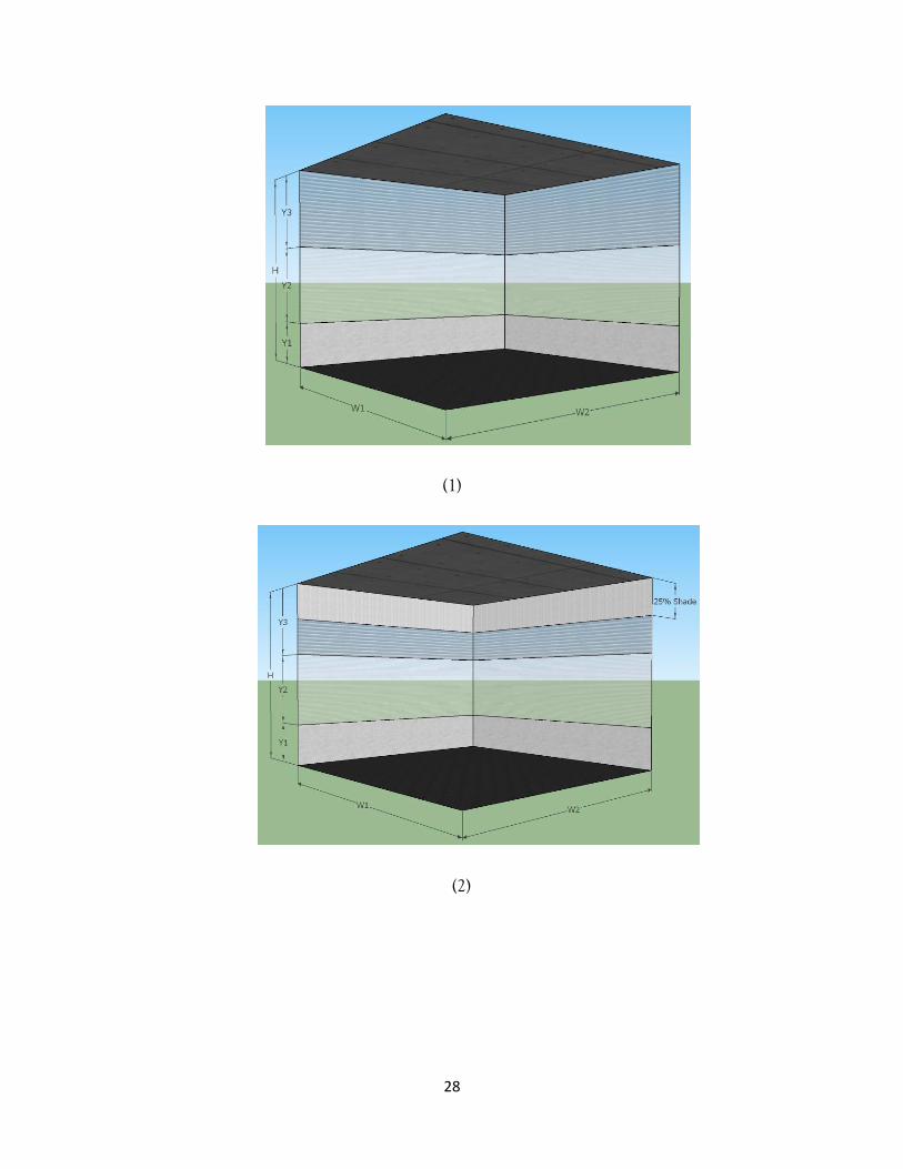
To simulate the daylight distribution, five different configurations of shading position

(Figure: 16) were implied. Cases considered included no shade (0% shade i.e. fully open),

25% shade, 50% shade, 75% shade and fully closed means 100% shade.

28

(1)

(2)

29

(3)

(4)

30

(5)

Figure 16: Shading position configurations

3.6 Daylight Glare Probability (DGP)

Daylight glare probability (DGP) (Wienold and Christoffersen 2006) is a matrix commonly

used for classify the glare produced by sunlight. DGP is calculated by the position, size and

luminance of the source and the vertical eye illuminance. DGP under 0.3 is considered barely

perceptible, from 0.3 to 0.45 is disturbing and over 0.45 is intolerable (Athienitis and O'Brien

2015). The DGP can be calculated by the following equation:

𝐷𝐺𝑃 = 5.87 × 10−5 𝐸𝑣 + 9.18 × 10−2𝑙𝑜𝑔 (1 + ∑𝐿𝑠,𝑖

2 𝜔𝑠,𝑖

𝐸𝑣1.87𝑃𝑖

2𝑖 ) + 0.16 (19)

where, Ev is the vertical eye illuminance, Ls is the source luminance, 𝜔𝑠 is the solid angle of

the source from the observer, P is the position index of the observer.

31

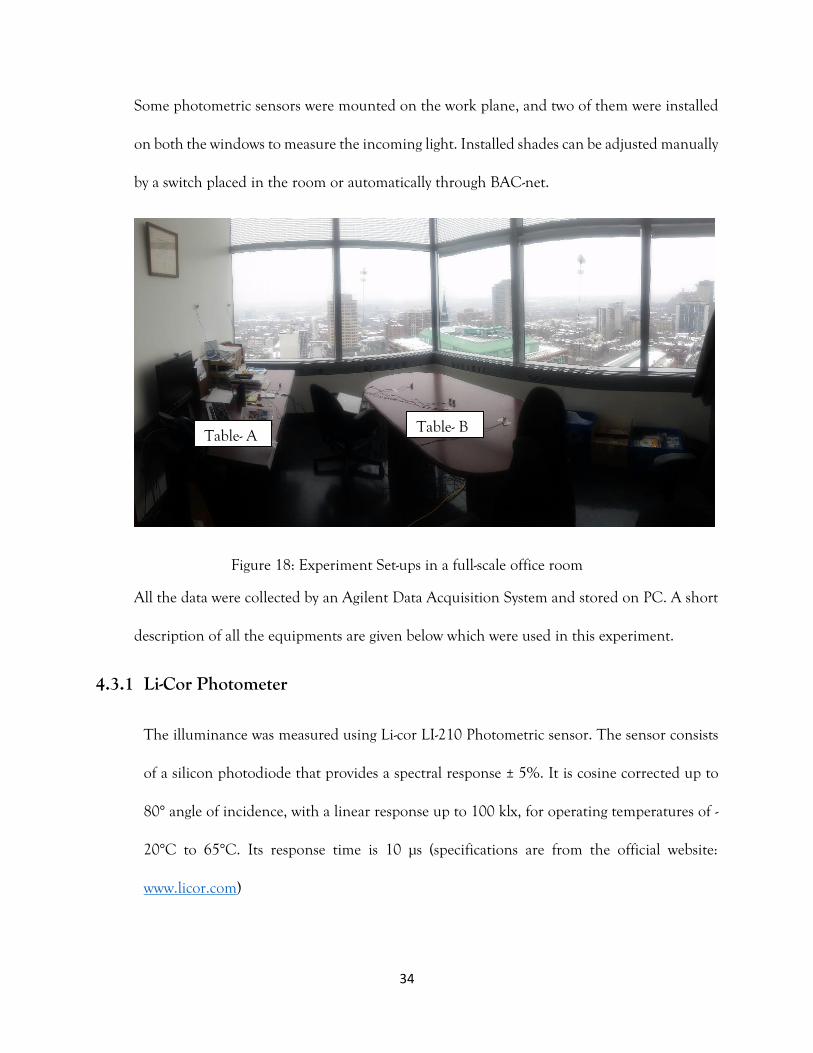
When the position index (P) is located above the line of vision, that can be calculated as

follows:

ln 𝑃 = [35.2 − 0.31889𝜏 − 1.22𝑒−2𝜋

9 ] × 10−3𝜎 + [21 + 0.26667𝜏 − 0.002963𝜏2] × 10−5𝜎2 (20)

where 𝜏 is the angle from the vertical of plane containing source and line of sight, 𝜎 is the

angle between line of sight and line from eye to source.

If the position index (P) is located below the line of vision, that be calculated as follows:

𝑃 = 1 + 0.8 𝑅

𝐷 𝑖𝑓 𝑅 > 0.6𝐷 (21)

𝑃 = 1 + 1.2 𝑅

𝐷 𝑖𝑓 𝑅 < 0.6𝐷 (22)

𝑅 = √𝐻2 + 𝑌2 (23)

where D is the distance between eye and plane of source in the direction of view, H is the

vertical distance between source and the view direction and Y is the horizontal distance

between the source and view direction.

32

Chapter 4: Experiment and model verification

4.1 Introduction

In order to verify the model, an experiment was conducted in a typical office room located on

the 15th floor of Concordia University, Montreal (45.50 N, 740 W). During experimentation,

an acceptable work plane illuminance for the office was maintained. The surface azimuth of

the two façades are 200 west of south and 1100 west of south. On both sides of the façade,

there are no external visual obstacles.

Figure 17: Engineering and visual Arts (EV) building, Concordia University, Montreal, QC (www.concordia.ca).

33

The primary objectives of the experiment were:

Compare the simulated data with the real data (Overcast and sunny sky conditions)

and validate the radiosity model and its assumptions

Analyzing the daylight distribution on the typical room

Parametric analysis with different properties of the room and the shading devices

4.2 Properties of the room components

Each façade consists of three sections, the opaque spandrel (0.8m from the floor), the lower

clear glass section (double-glazed with a low emissivity coating) and the upper fritted glass

section (50% gray ceramic frit). Each glazing is 1.25 m high. A motorized roller shade was

installed above the glazing. The reflectance of the walls, floor, and ceiling, are 70%, 5% and

80% respectively. The clear and fritted glazing have a normal visible transmittance of 68% and

48% respectively.

4.3 Experimental set-up

A corner office in the Concordia EV building was used for model verification. The building

has façades with complete measurement setups of exterior solar radiation and daylight. Several

equipment were installed for the experiment. For measuring the illuminance, a number of Li-

Cor Photometric sensors (Model LI-2100R, by LI-COR) were installed at work plane height

(0.8 m). For data acquisition, an Agilent DAS unit was used. The roller shades were already

installed at that office room.

34

Some photometric sensors were mounted on the work plane, and two of them were installed

on both the windows to measure the incoming light. Installed shades can be adjusted manually

by a switch placed in the room or automatically through BAC-net.

Figure 18: Experiment Set-ups in a full-scale office room

All the data were collected by an Agilent Data Acquisition System and stored on PC. A short

description of all the equipments are given below which were used in this experiment.

4.3.1 Li-Cor Photometer

The illuminance was measured using Li-cor LI-210 Photometric sensor. The sensor consists

of a silicon photodiode that provides a spectral response ± 5%. It is cosine corrected up to

80° angle of incidence, with a linear response up to 100 klx, for operating temperatures of -

20°C to 65°C. Its response time is 10 µs (specifications are from the official website:

www.licor.com)

Table- A Table- B

http://www.licor.com/

35

Figure 19: Li-cor LI-210 Photometric sensor

4.3.2 Data Acquisition System

Agilent Data Acquisition system was used in this experiment. It is generally used for data

acquisition with a variety of plug-in modules known as thermocouple multiplexer.

The data were collected through a Lab View program to a computer connected to the data

acquisition system.

4.3.3 Façade

The three sections of the façade consist of an opaque spandrel, one clear glass section, and

one fritted glass section. Both the glass sections are made of double glazing, low e-coated and

argon gas filled. The clear and fritted glazing have a normal visible transmittance of 68% and

48% respectively for the diffused light (Kapsis 2009).

For the direct sunlight, the transmittance of both the glasses depends on the angle of

incidence of the solar radiation on the glazing.

4.3.4 Shades

A set of pre-installed roller shades were used for the experiment. This roller shade is

connected to a BAC-net system and automatic and manually operated. The shades are

36

installed just in front of the windows and is made of fabric. The optical properties of the

fabric are as follows:

Transmittance = 5%

Reflectance = 55%

4.4 Sensor positioning

To take the measurement two sensors (sensor 1 and sensor 2) were placed on the meeting

table (Table: B). Two sensors (sensor 3 and sensor 4) were placed on the working desk (Table:

A). One sensor (sensor 5) was set on just top of the monitor and attached to the north wall.

Two sensors (sensor 6 and sensor 8) were placed close to the south and east façade. One sensor

(sensor 7) was set on the south façade to measure the illuminance at the window.

The schematics of the position of the sensors are given below (Figure 20 and 21):

Figure 20: Schematic of the sensor position on the work plane.

1m

1 2

3 4

8

6

2m

1.5m 1.5m

1m

1.5m

37

Figure 21: Schematic of the sensor position on the windows

4.5 Experimental verification on overcast day

Measurements were taken at different points on the work plane on many days with varying

shade position configurations. The area-weighted properties (e.g. to account for furniture) of

the room surfaces, glazing and shades were used in this model. The work plane illuminance

values were measured using LI-COR light sensors installed on the work plane (0.8 m from the

floor)

This experiment was conducted to consider overcast days. This verification has been carried

out on four selected points on the work plane.

7 5

1.5m

38

Figure 22: Selected points of measurement on the work plane

After taking data for several overcast and sunny days, some data had been chosen for the

verification. Table 2 shows the simulated and measured illuminance for different shading

position at different places on the work plane.

Table: 2: Simulated and measured illuminance for different shading position at different

places on the work plane.

Shade Position

Point 9 Point 7 Point 12 Point 19

S (lx) M (lx) S (lx) M (lx) S (lx) M (lx) S (lx) M (lx)

0% (open) 6873 6677 8442 8516 7615 7945 5330 5240

25% 6030 5943 7648 8190 6708 6806 4371 4024

50% 4990 3822 6532 5988 5513 5165 3323 2488

75% 4147 3712 5825 5831 4709 5120 2303 2854

100% (closed)

204 203 225 242 249 251 226 223

39

When a linear regression was plotted (Figure 22) for the measured and simulated

illuminance data, it is seen that the coefficient of determination (R2) for the curve is 0.97,

which is very much acceptable.

Figure 23: Measured vs simulated data of illuminance on work-plane (lux)

Figures 24-28 show the simulated and measured illuminance on the work plane for five

different shade positions (all open, 25%, 50%, 75% and all shades closed) individually. The

comparison of simulation results and measured data show that for an overcast day, the

simulation results on average differ 1-10% from the measured data which is an acceptable

agreement. Because of the shape, the interior surfaces, furniture inside the room and

occupant’s presence, this accuracy level is being considered as acceptable. Moreover,

sometimes real sky condition is quite different from the simulation due to a different

circumstance, such as cloud cover. For this reason, in some cases, the simulated result

appears higher than the measured value (such as the 50% shade condition).

0

1000

2000

3000

4000

5000

6000

7000

8000

9000

10000

0 2500 5000 7500 10000

Mea

sure

d Il

lum

ian

ance

Simulated Illumianance

40

Figure 24: Illuminance comparison for all open shade configuration

Figure 25: Illuminance comparison for 25% shade configuration

0

1000

2000

3000

4000

5000

6000

7000

8000

9000

10000


Illu

min

ance

(lx

)

Simulation Measured

0

1000

2000

3000

4000

5000

6000

7000

8000

9000

10000


Illu

min

ance

(lx

)

Simulation Measured

41



0

1000

2000

3000

4000

5000

6000

7000

8000

9000

10000


Illu

min

ance

(lx

)

Simulation Measured

0

1000

2000

3000

4000

5000

6000

7000

8000

9000

10000


Illu

min

ance

(lx

)

Simulation Measured

42

Figure 28: Illuminance comparison for all closed shade configuration

4.6 Parametric Analysis

Changing the optical properties of the glazing, shades and room surfaces, we can predict the

daylight distribution for any enclosed spaces. Having façade on two sides makes the model

more generalized, as one façade on either orientation can also be analyzed.

After verifying the model, parametric simulations were performed for varying floor reflectance

to investigate the effect on work plane illuminance level. The effect of transmittance of the

shades was also analyzed for various configurations and the effect of two different shades in

two sections of each façade. The configuration with higher transmittance on the upper section

and lower transmittance on the lower section of the façade show a significant effect on

illuminance. This is acceptable because in the middle viewing section of the facade we cannot

have a high transmittance for privacy reasons; however, in the top third of the facade, we have

0

50

100

150

200

250

300


Illu

min

ance

(lx

)

Simulation Measured

43

more flexibility in using a higher transmittance so as to have more daylight penetrate deep

into the room. This is a particularly important aspect of the model and this study.

The floor of the corner office where the experiments took place, has a low optical reflectance

of 5%. Many offices have lighter colored floors with higher reflectance. A sensitivity analysis

on floor reflectance was performed with reflectance varying from 5% to 50% in 5% increments

(normally a floor reflectance above 30% is not advisable in offices). The results suggest an 8-

12% increase in work plane illuminance due to the variation of the floor reflectance from 5%

to 50%. The analysis was performed for all shades open (Figure 29) and all shades closed

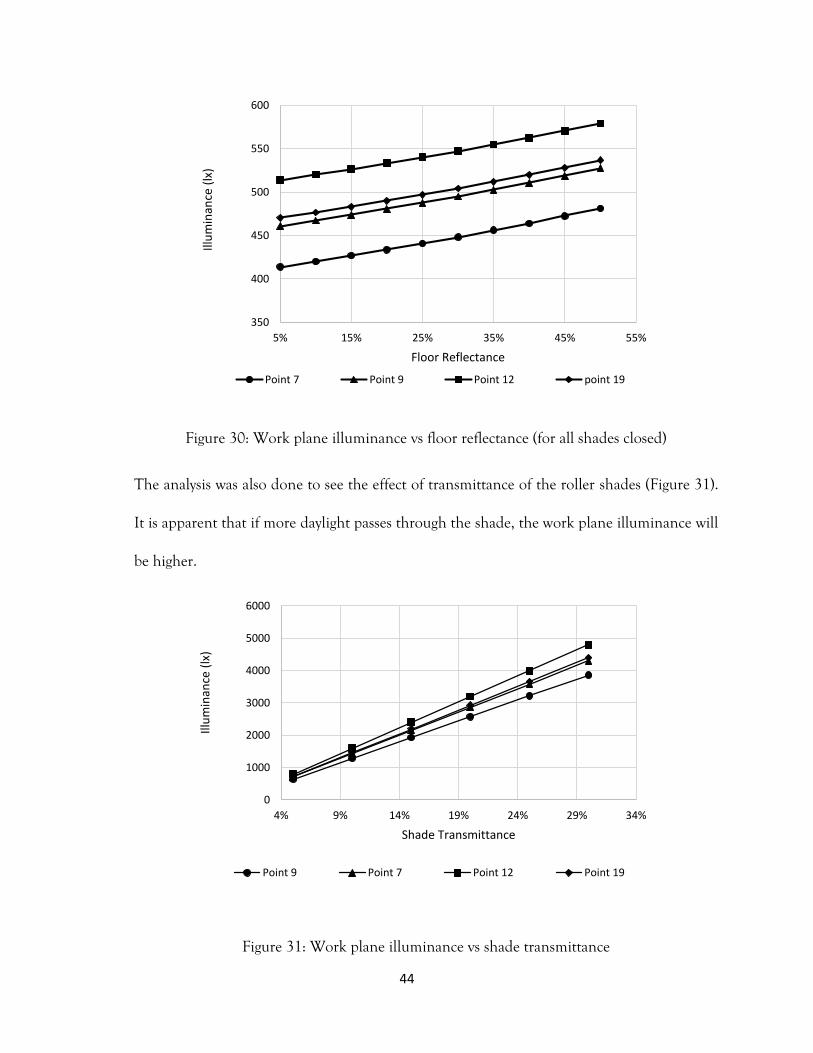
(Figure 30).

Figure 29: Work plane illuminance vs floor reflectance (for all shades open)

3500

3700

3900

4100

4300

4500

4700

4900

5100

5300

5500

5% 15% 25% 35% 45% 55%

Illu

min

ance

(lx

)

Floor Reflectance


44

Figure 30: Work plane illuminance vs floor reflectance (for all shades closed)

The analysis was also done to see the effect of transmittance of the roller shades (Figure 31).

It is apparent that if more daylight passes through the shade, the work plane illuminance will

be higher.

Figure 31: Work plane illuminance vs shade transmittance

350

400

450

500

550

600

5% 15% 25% 35% 45% 55%

Illu

min

ance

(lx

)

Floor Reflectance

Point 7 Point 9 Point 12 point 19

0

1000

2000

3000

4000

5000

6000

4% 9% 14% 19% 24% 29% 34%

Illu

min

ance

(lx

)

Shade Transmittance


45

The primary purpose of windows on perimeter façade are to provide daylight in to the space

and for outdoor view. But privacy of the occupants working close to the façade is also an

important issue now a days. There are different ideas of privacy. Some people wants to block

the full view from outside and for some people the view of shadows from outside is preferable.

To block the complete view from outside, a blackout shade is preferable. But for other option

shades with lower transmittance can be used. However when blackout shades are closed, the

outdoor view and also natural light is being sacrificed.

To see the various options of shading, balancing the daylighting through upper part of the

façade and maintaining privacy by middle part of the façade, another parametric simulation

was done varying the transmittance of the shades on different sections of façade. This

simulation was performed with the top part of the façade transmittance varying from 1% to

25% and middle part of the façade transmittance varying from 1% to 10%. A fabric with 1%

transmittance provides more privacy and less light than a fabric with 10% transmittance. This

simulation was done for three types of room geometry.

Windows on near-south and near-east facades (Figure 32).

Window on near-east façade only (Figure 33).

Window on near-south façade only (Figure 34).

46

Figure 32: Work-plane illuminance due to different shade transmittance on different sections of near-south and near-east facades.

47

Figure 33: Work-plane illuminance due to different shade transmittance on different sections of near-east façade (Considering near-south facade is opaque).

48

Figure 34: Work-plane illuminance due to different shade transmittance on different sections of near-south façade (Considering near-east facade is opaque).

Figures 32 - 34 show the results in the morning (10 AM) on a clear sky day for a range of

transmittance values of the shade in the top and middle facade sections. As can be seen,

acceptable work-plane illuminance levels (>2000 lx) can be maintained by using different

shades on upper and middle portion of the façade. From the graphs, the right combination of

shade transmittance can be determined depending the needs of the occupants, whether they

need the privacy or the daylight or both. This types of configuration of shading can also reduce

the glare caused by the direct sunrays.

49

A daylight glare probability (DGP) analysis has been done on the work-plane (Table-B of figure

18) level for three types of room geometry mentioned above with different shade

transmittances on different sections of the façade to determine the limit of the maximum

transmittance for the shades so as to avoid glare. DGP is determined from the luminance of

the diffuse source (windows with all shades closed) and the vertical illuminance on the work-

plane. DGP is used to classify the glare range. DGP under 0.3 is considered barely perceptible

(i.e. it is acceptable), from 0.3 to 0.45 it is disturbing and over 0.45 is intolerable (Athienitis

and O'Brien 2015).

Figures 35-37 show the results for calculated DGP on a typical clear sky day (9 June, 10 AM)

on the work-plane. From the figures, the maximum limit can be determined for both shade

transmittances on top and middle section of each façade. Depending on the occupant’s need,

whether the privacy or the daylight is needed, the transmittance of the shades can be set

accordingly. To calculate the DGP no veiling glare was taken into account assuming there are

no internal reflections from the computer monitor or from any other surfaces.

50

Figure 35: Calculated Daylight Glare Probability (DGP) for different shade transmittances on different sections of both façades.

51

Figure 36: Calculated Daylight Glare Probability (DGP) for different shade transmittances on different sections of near-east façade (Considering near-south facade is opaque).

52

Figure 37: Calculated Daylight Glare Probability (DGP) for different shade transmittances on different sections of near-south façade (Considering near-east facade is opaque).

From the figures it can be clearly seen that, maintaining the privacy of the occupant with lower transmittance on the middle section of the façade, we can use the shade on the upper part with higher transmittance. Considering the shade transmittance of the middle section as 5%, the maximum limit for the shade transmittance of the top part of the façade can be 15% (Figure 35) to avoid glare.

For two other types of room geometry where only one façade is considered, it can be seen from the simulation that, the maximum limit of shade transmittance for the top section can be over 20%.

The DGP values for combination of shades with different transmittances are listed on appendix A, B and C.

53

Chapter 5: Conclusion

5.1 Conclusions

In this thesis, a generalized radiosity model is presented for a corner office having three section

façade. The three section façade (Kapsis et al. 2015) consists of a lower part of the opaque

(spandrel) panel, a middle section of clear glazing and an upper section of fritted glass. The

model is verified with experimental measurements for a zone with up to two glazed 3-section

facades with the possibility of two types of shades. The model was then extended to simulate

various scenarios of interest. This model was designed specifically for a corner office, but can

be easily adjusted to model any room in a perimeter zone of a building having its façade in

any orientation.

A fourteen-surface room enclosure was considered to calculate the view factor of the room.

The main input parameters for this model are i) the geographic location, ii) the room

dimension, iii) the reflectance of the interior surfaces, glazing and shades, iv) the visible

transmittance of the glazing and shades, and v) the sky condition.

To simulate the daylight distribution, five different configurations of shading position were

implied. Those includes, no shade (0% shade i.e. fully open), 25% shade, 50% shade, 75%

shade and fully closed means 100% shade.

The model was then verified by conducting a full scale experiment. For the experiment, a full-

scale office room with windows on two adjacent façades was used. The experiment validates

the model with all shading position for an overcast sky condition.

54

Comparing the simulated results and measured data for an overcast day, it is found that the

simulation results on average differ 1-10% from the measured data which is an acceptable

agreement, because of the shape, the interior surfaces, furniture inside the room and

occupant’s presence.

A model parametric study and the simulation results of the effect of floor reflectance, shade

transmittance was also performed. The results suggest an 8-12% increase in work plane

illuminance due to the variation of the floor reflectance from 5% to 50%.

Using low transmittance shades for privacy reasons in the middle section of a 3-section facade

and a higher transmittance in the top section for deep daylight penetration allows for more

flexibility in daylight design; some of the low sunlight can be blocked while providing overall

increased daylight utilization and occupant privacy. The daylight glare probability (DGP)

shows that, on a clear sky assuming all transmitted sunlight is diffused and with all shades are

closed, high transmittance for the top section with maximum limit of 15% is ideal to avoid

glare while keeping the privacy at the same time by installing a shade with 5% transmittance

at the middle section.

DGP analysis also shows that, having windows on one façade can maximize the limit for shade

transmittances on both sections of the façade.

55

5.2 Future Work

As the modern architectural building uses perimeter zones of the building for as the main

path to allow daylights in the buildings, it has become more important to study the

distribution of daylight in every corner of the buildings. It helps to reduce the electric energy

for artificial lighting as well as contributes to design the HVAC system.

As this radiosity model is only validated for overcast sky condition, a further study can be done

for the sunny day with diffuse and direct sunlight.

The top fritted part of the windows can be installed with semi-transparent photovoltaics to

generate electricity while allowing some sunlight to the room, leaving the middle section for

outdoor views or shaded as occupants need. The experiment can further be extended to

various dimensionless design parameter ranges such as 𝑊1

𝑊2,

𝑊1

𝐻,

𝑊2

𝐻 , façade aspect ratio (such

as 𝑌1

𝐻,

𝑌2

𝐻,

𝑌3

𝐻).

Finally, an improved control strategy can be development to reduce glare and excessive lighting

and heat gain by controlling the shades to desired positions.

56

References

1. Energy Use Data Handbook 2009-2013, Natural Resources Canada.

2. Athienitis, A. (1999). Building Tharmal Analysis. Boston, U.S.A., Mathsoft Inc.

3. Athienitis, A. and W. O'Brien (2015). Modeling, Design, and Optimization of Net-Zero

Energy Buildings, Ernst & Sohn.

4. Athienitis, A. K. and U. Boxer (2001). Effect of numerical model detail on prediction of

interior illumination levels. Canadian Congress of Applied Mechanics. Monteal, QC.

5. Athienitis, A. K. and M. Santamouris (2002). Thermal Analysis and Design of Passive Solar

Buildings, James & James.

6. Athienitis, A. K. and A. Tzempelikos (2002). "A methodology for simulation of daylight

room illuminance distribution and light dimming for a room with a controlled shading

device." Solar Energy 72(4): 271-281.

7. Bellia, L., et al. (2014). "Overview on Solar Shading Systems for Buildings." Energy Procedia

62: 309-317.

8. Boyce, P., et al. (2003). The Benefits of Daylight Through Windows. Troy, New York,

Lighting Research Center, Rensselaer Polytechnic Institute.

9. Chan, Y.-C. and A. Tzempelikos (2012). A Hybrid Ray-Racing and Radiosity Method for

Calculating Radiation Transport and Illuminance Distribution in Spaces With Venetian

Blinds. International High Performance Buildings Conference. Purdue,: 3220 (3221-3210).

10. Escuyer, S. and M. Fontoynont (2001). "Lighting controls: a field study of office workers’

reactions." Lighting Research and Technology 33(2): 77-94.

57

11. Farley, K. M. J. and J. A. Veitch (2001). A Room With A View: A Review of the Effects of

Windows on Work and Well-Being. Research Report, NRC Institute for Research in

Construction; 136.

12. Glassner, A. S., Ed. (1989). An introduction to ray tracing. London, UK, Academic Press

Ltd.

13. Heschong, L., et al. (2002). "Daylighting Impacts on Human Performance in School." Journal

of the Illuminating Engineering Society 31(2): 101-114.

14. Kapsis, K. (2009). Modeling, Control & Performance Evaluation of Bottom‐up Motorized

Shade. Building, Civil, and Environmental Engineering. Montreal, Quebec, Canada,

Concordia University. Master of Applied Science.

15. Kapsis, K. and A. K. Athienitis (2015). "A study of the potential benefits of semi-transparent

photovoltaics in commercial buildings." Solar Energy 115: 120-132.

16. Kapsis, K., et al. (2015). "Daylight Performance of Perimeter Office Façades utilizing Semi-

transparent Photovoltaic Windows: A Simulation Study." 6th International Building Physics

Conference, IBPC 2015 78: 334-339.

17. Kapsis, K., et al. (2010). "Daylighting performance evaluation of a bottom-up motorized

roller shade." Solar Energy 84(12): 2120-2131.

18. Kuhn, T. E., et al. (2001). "Evaluation of overheating protection with sun-shading systems."

Solar Energy 69, Supplement 6: 59-74.

19. Lee, E. S., et al. (1998). "Thermal and daylighting performance of an automated venetian

blind and lighting system in a full-scale private office." Energy and Buildings 29(1): 47-63.

58

20. Lehar, M. A. and L. R. Glicksman (2007). "Rapid algorithm for modeling daylight

distributions in office buildings." Building and Environment 42(8): 2908-2919.

21. Mettanant, V. and P. Chaiwiwatworakul (2014). "Automated Vertical Blinds for Daylighting

in Tropical Region." Energy Procedia 52: 278-286.

22. Mills, L. R. and W. R. McCluney (1993). "The benefits of using window shades." ASHRAE

Journal (American Society of Heating, Refrigerating and Air-Conditioning Engineers) 35:11:

20-27.

23. Morini, G. L., et al. (2014). "Internal Versus External Shading Devices Performance in Office

Buildings." Energy Procedia 45: 463-472.

24. Mukherjee, S., et al. (2010). "Closed Loop Integrated Lighting and Daylighting Control for

Low Energy Buildings." ACEEE Summer Study on Energy Efficiency in Buildings 9: 252-

269.

25. Muller, S., et al. (1995). A radiosity approach for the simulation of daylight. Rendering

Techniques. Dublin, Ireland: 12-14.

26. Murdoch, J. B. (2003). Illuminating Engineering: From Edison's Lamp to the LED, Visions

Communications.

27. Perez, R., et al. (1990). "Modeling daylight availability and irradiance components from

direct and global irradiance." Solar Energy 44(271-289).

28. Reinhart, C. F. and K. Voss (2003). "Monitoring manual control of electric lighting and

blinds." Lighting Research and Technology 35(3): 243-258.

29. Robinson, D. and A. Stone (2006). "Internal illumination prediction based on a simplified

radiosity algorithm." Solar Energy 80(3): 260-267.

59

30. Shen, E., et al. (2014). "Energy and visual comfort analysis of lighting and daylight control

strategies." Building and Environment 78: 155-170.

31. Shen, H. and A. Tzempelikos (2014). A Global Method for Efficient Synchronized Shading

Control Using the “Effective daylight” Concept. 3rd International High Performance

Buildings Conference. Purdue.

32. Skelly, M. J. and M. A. Wilkinson (2001). "The evolution of interactive facades: improving

automated blind control." Whole life performance of facades: 129-142.

33. Tzempelikos, A., et al. (2007). Daylight and luminaire control in a perimeter zone using an

automated venetian blind. 28th AIVC Conference on Building Low Energy Cooling and

Advanced Ventilation Technologies in the 21st Century. Crete island, Greece.

34. Vine, E., et al. (1998). "Office worker response to an automated Venetian blind and electric

lighting system: a pilot study." Energy and Buildings 28(2): 205-218.

35. Wienold, J. and J. Christoffersen (2006). "Evaluation methods and development of a new

glare prediction model for daylight environments with the use of CCD cameras." Energy and

Buildings 38(7): 743-757.

60

Appendix A

Calculated Daylight Glare Probability (DGP) for different shade transmittances on different sections of both façade.

Upper Lower (1%)

Lower (2%)

Lower (3%)

Lower (4%)

Lower (5%)

Lower (6%)

Lower (7%)

Lower (8%)

Lower (9%)

Lower (10%)

1% 0.177 0.189 0.201 0.212 0.224 0.236 0.248 0.26 0.271 0.283

2% 0.182 0.194 0.206 0.218 0.229 0.241 0.253 0.265 0.277 0.288

3% 0.187 0.199 0.211 0.223 0.235 0.246 0.258 0.27 0.282 0.293

4% 0.193 0.204 0.216 0.228 0.24 0.251 0.263 0.275 0.287 0.299

5% 0.198 0.209 0.221 0.233 0.245 0.257 0.268 0.28 0.292 0.304

6% 0.203 0.215 0.226 0.238 0.25 0.262 0.274 0.285 0.297 0.309

7% 0.208 0.22 0.232 0.243 0.255 0.267 0.279 0.29 0.302 0.314

8% 0.213 0.225 0.237 0.248 0.26 0.272 0.284 0.296 0.307 0.319

9% 0.218 0.23 0.242 0.254 0.265 0.277 0.289 0.301 0.312 0.324

10% 0.224 0.235 0.247 0.259 0.271 0.282 0.294 0.306 0.318 0.329

11% 0.229 0.24 0.252 0.264 0.276 0.287 0.299 0.311 0.323 0.335

12% 0.234 0.246 0.257 0.269 0.281 0.293 0.304 0.316 0.328 0.34

13% 0.239 0.251 0.262 0.274 0.286 0.298 0.31 0.321 0.333 0.345

14% 0.244 0.256 0.268 0.279 0.291 0.303 0.315 0.326 0.338 0.35

15% 0.249 0.261 0.273 0.284 0.296 0.308 0.32 0.332 0.343 0.355

16% 0.254 0.266 0.278 0.29 0.301 0.313 0.325 0.337 0.348 0.36

17% 0.26 0.271 0.283 0.295 0.307 0.318 0.33 0.342 0.354 0.365

18% 0.265 0.276 0.288 0.3 0.312 0.323 0.335 0.347 0.359 0.371

19% 0.27 0.282 0.293 0.305 0.317 0.329 0.34 0.352 0.364 0.376

20% 0.275 0.287 0.298 0.31 0.322 0.334 0.346 0.357 0.369 0.381

21% 0.28 0.292 0.304 0.315 0.327 0.339 0.351 0.362 0.374 0.386

22% 0.285 0.297 0.309 0.321 0.332 0.344 0.356 0.368 0.379 0.391

23% 0.29 0.302 0.314 0.326 0.337 0.349 0.361 0.373 0.385 0.396

24% 0.296 0.307 0.319 0.331 0.343 0.354 0.366 0.378 0.39 0.401

25% 0.301 0.312 0.324 0.336 0.348 0.359 0.371 0.383 0.395 0.407

61

Appendix B

Calculated Daylight Glare Probability (DGP) for different shade transmittances on different sections of east façade (Considering south facade is opaque).

Upper Lower (1%)

Lower (2%)

Lower (3%)

Lower (4%)

Lower (5%)

Lower (6%)

Lower (7%)

Lower (8%)

Lower (9%)

Lower (10%)

1% 0.177 0.182 0.187 0.192 0.197 0.202 0.206 0.211 0.216 0.22

2% 0.179 0.183 0.188 0.193 0.198 0.203 0.208 0.213 0.217 0.222

3% 0.181 0.185 0.19 0.195 0.2 0.205 0.21 0.214 0.219 0.224

4% 0.183 0.187 0.192 0.197 0.202 0.207 0.211 0.216 0.221 0.226

5% 0.186 0.19 0.194 0.199 0.204 0.208 0.213 0.218 0.223 0.228

6% 0.188 0.192 0.196 0.201 0.205 0.21 0.215 0.22 0.225 0.229

7% 0.191 0.194 0.198 0.203 0.207 0.212 0.217 0.222 0.227 0.231

8% 0.193 0.196 0.2 0.205 0.209 0.214 0.219 0.224 0.228 0.233

9% 0.195 0.199 0.203 0.207 0.212 0.216 0.221 0.226 0.23 0.235

10% 0.197 0.201 0.205 0.209 0.214 0.218 0.223 0.228 0.232 0.237

11% 0.199 0.203 0.207 0.211 0.216 0.22 0.225 0.23 0.234 0.239

12% 0.202 0.205 0.209 0.213 0.218 0.222 0.227 0.232 0.236 0.241

13% 0.204 0.207 0.211 0.216 0.22 0.225 0.229 0.234 0.238 0.243

14% 0.206 0.21 0.214 0.218 0.222 0.227 0.231 0.236 0.241 0.245

15% 0.208 0.212 0.216 0.22 0.224 0.229 0.233 0.238 0.243 0.247

16% 0.21 0.214 0.218 0.222 0.226 0.231 0.235 0.24 0.245 0.249

17% 0.212 0.216 0.22 0.224 0.229 0.233 0.238 0.242 0.247 0.251

18% 0.214 0.218 0.222 0.226 0.231 0.235 0.24 0.244 0.249 0.253

19% 0.216 0.22 0.224 0.229 0.233 0.237 0.242 0.246 0.251 0.255

20% 0.219 0.222 0.227 0.231 0.235 0.239 0.244 0.248 0.253 0.258

21% 0.221 0.225 0.229 0.233 0.237 0.242 0.246 0.25 0.255 0.26

22% 0.223 0.227 0.231 0.235 0.239 0.244 0.248 0.253 0.257 0.262

23% 0.225 0.229 0.233 0.237 0.241 0.246 0.25 0.255 0.259 0.264

24% 0.227 0.231 0.235 0.239 0.244 0.248 0.252 0.257 0.261 0.266

25% 0.229 0.233 0.237 0.241 0.246 0.25 0.254 0.259 0.263 0.268

62

Appendix C

Calculated Daylight Glare Probability (DGP) for different shade transmittances on different sections of south façade (Considering east facade is opaque).

Upper Lower (1%)

Lower (2%)

Lower (3%)

Lower (4%)

Lower (5%)

Lower (6%)

Lower (7%)

Lower (8%)

Lower (9%)

Lower (10%)

1% 0.17 0.178 0.185 0.192 0.199 0.206 0.213 0.22 0.227 0.234

2% 0.174 0.181 0.188 0.195 0.202 0.209 0.216 0.223 0.23 0.238

3% 0.177 0.184 0.191 0.198 0.205 0.212 0.219 0.226 0.233 0.241

4% 0.18 0.187 0.194 0.201 0.208 0.215 0.222 0.229 0.237 0.244

5% 0.183 0.19 0.197 0.204 0.211 0.218 0.225 0.233 0.24 0.247

6% 0.186 0.193 0.2 0.207 0.214 0.221 0.229 0.236 0.243 0.25

7% 0.189 0.196 0.203 0.21 0.217 0.225 0.232 0.239 0.246 0.253

8% 0.192 0.199 0.206 0.213 0.22 0.228 0.235 0.242 0.249 0.256

9% 0.195 0.202 0.209 0.217 0.224 0.231 0.238 0.245 0.252 0.259

10% 0.198 0.205 0.213 0.22 0.227 0.234 0.241 0.248 0.255 0.262

11% 0.202 0.209 0.216 0.223 0.23 0.237 0.244 0.251 0.258 0.265

12% 0.205 0.212 0.219 0.226 0.233 0.24 0.247 0.254 0.261 0.268

13% 0.208 0.215 0.222 0.229 0.236 0.243 0.25 0.257 0.264 0.271

14% 0.211 0.218 0.225 0.232 0.239 0.246 0.253 0.26 0.267 0.275

15% 0.214 0.221 0.228 0.235 0.242 0.249 0.256 0.263 0.271 0.278

16% 0.217 0.224 0.231 0.238 0.245 0.252 0.259 0.267 0.274 0.281

17% 0.22 0.227 0.234 0.241 0.248 0.255 0.263 0.27 0.277 0.284

18% 0.223 0.23 0.237 0.244 0.251 0.259 0.266 0.273 0.28 0.287

19% 0.226 0.233 0.24 0.248 0.255 0.262 0.269 0.276 0.283 0.29

20% 0.23 0.237 0.244 0.251 0.258 0.265 0.272 0.279 0.286 0.293

21% 0.233 0.24 0.247 0.254 0.261 0.268 0.275 0.282 0.289 0.296

22% 0.236 0.243 0.25 0.257 0.264 0.271 0.278 0.285 0.292 0.299

23% 0.239 0.246 0.253 0.26 0.267 0.274 0.281 0.288 0.295 0.302

24% 0.242 0.249 0.256 0.263 0.27 0.277 0.284 0.291 0.298 0.306

25% 0.245 0.252 0.259 0.266 0.273 0.28 0.287 0.294 0.302 0.309

63

Appendix D

Radiosity Simulation Model

A RADIOSITY MODEL OF A CORNER OFFICE ROOM

Parameters :

Location :

Latitude: L 45.5 deg⋅:= Local standard time meridian: STM 75 deg⋅:=

Longitude: LNG 74 deg⋅:= Window surface azimuth: ψs 20− deg⋅:=

The surface tilt angle of the window is: βw 90deg:=ψe 110− deg⋅:=

Representative days

Equinox

Summer_Solstice

Winter_Solstice

Winter_Sunny

Winter_Overcast

Summer_Sunny

Summer_Overcast

79

172

355

13

39

243

170

:=

Selected day

n 161:= ...... June 09, 2015

Solar geometry

Fig.1 Solar geometry (Athienitis, 1998)

64

Equation of time (ET):

ET n( ) 9.87 sin 4 π⋅n 81−

364⋅

⋅ 7.53 cos 2 π⋅n 81−

364⋅

⋅− 1.5 sin 2 π⋅n 81−

364⋅

⋅−

min⋅:=

Apparent Solar Time (AST):

AST n t, ( ) t hr⋅ ET n( )+STM LNG−( ) hr⋅

15 deg⋅+:= s n t, ( ) AST n t, ( ) 12 hr⋅−:=

Solar declination (δ ) :

δ n( ) 23.45 deg⋅ sin 360284 n+

365⋅ deg⋅

⋅:=

Hour angle (H):

H n t, ( ) AST n t, ( ) 12 hr⋅−( ) 15deg

hr⋅

⋅:=

Sunset hour angle ( hs ) :

hs n( ) acos tan L( )− tan δ n( )( )⋅( )( ):=

Sunset time ( ts ) :

ts n( ) hs n( )hr

15 deg⋅⋅:=

Surface sunset time ( tss ) :

tss n( ) min hs n( ) acos tan L βw−( )− tan δ n( )( )⋅( )( )( )hr

15 deg⋅⋅:=

Solar altitude (αs ) :

αs n t, ( ) asin cos L( )( ) cos δ n( )( )⋅ cos H n t, ( )( )⋅sin L( )( ) sin δ n( )( )⋅+

...

asin cos L( )( ) cos δ n( )( )⋅ cos H n t, ( )( )⋅sin L( ) sin δ n( )( )⋅+

...

0 deg⋅>if

0 deg⋅ otherwise

:=

Solar azimuth (φ ) :

ϕ n t, ( ) acossin αs n t, ( )( ) sin L( )⋅ sin δ n( )( )−

cos αs n t, ( )( ) cos L( )⋅

H n t, ( )

H n t, ( )⋅:=

Surface solar azimuth for south w indow (γs):

γs n t, ( ) ϕ n t, ( ) ψs−:=

Surface solar azimuth for east w indow (γe):

γe n t, ( ) ϕ n t, ( ) ψe−:=

Zenith angle (Z):

Z n t, ( ) acos cos L( ) cos δ n( )( )⋅ cos H n t, ( )( )⋅ sin L( ) sin δ n( )( )⋅+( )( ):=

65

Angle of incidence for south window (θs):

θθs n t, ( ) cos αs n t, ( )( ) cos γs n t, ( )( )⋅ sin βw( )⋅ sin αs n t, ( )( ) cos βw( )⋅+:=

θs n t, ( ) acosθθs n t, ( ) θθs n t, ( )+

2

:=

Angle of incidence for east window (θs):

θθe n t, ( ) cos αs n t, ( )( ) cos γe n t, ( )( )⋅ sin βw( )⋅ sin αs n t, ( )( ) cos βw( )⋅+:=

θe n t, ( ) acosθθe n t, ( ) θθe n t, ( )+

2

:=

Profile angle for south window ( ds):

ds n t, ( ) atantan αs n t, ( )( )cos γs n t, ( )( )

:=

Profile angle for east window (de):

de n t, ( ) atantan αs n t, ( )( )cos γe n t, ( )( )

:=

66

CIE Overcast Day

t 1 2, 24..:=

Lzst

123 8600 sin αs n t, ( )( )⋅+:=

Lsky_st

Lzst

31 2 cos θs n t, ( )( )⋅+( )⋅:=

Eho_st

7 π⋅

9Lzs

t⋅ lx⋅:=

10 200

5 103

×

1 104

×

1.5 104

×

2 104

×

Illuminance Incident on the facade

Time of the day

Illu

min

ance

(lx

)

Eho_st

t

Ed_southt

Eho_st

:=

Ed_eastt

Eho_st

:=

67

Visible transmittance of a double glazing window (Lower Facade):

Sd_pos_south 0:= Sd_pos_east 25:= ........ Select shade position (0%, 25%, 50%, 75%, 100%)

τshade 0.05:=

τs_lower_lt

τshade 0.69⋅ Sd_pos_south 100=if

0.69 otherwise

:=

τe_lower_lt

τshade 0.69⋅ Sd_pos_east 100=if

0.69 otherwise

:=

τs_lower_ut

τshade 0.69⋅ Sd_pos_south 100= Sd_pos_south 75=∨if

0.69 otherwise

:=

τe_lower_ut

τshade 0.69⋅ Sd_pos_east 100= Sd_pos_east 75=∨if

0.69 otherwise

:=

τs_upper_lt

τshade 0.48⋅ Sd_pos_south 100= Sd_pos_south 75=∨ Sd_pos_south 50=∨if

0.48 otherwise

:=

τe_upper_lt

τshade 0.48⋅ Sd_pos_east 100= Sd_pos_east 75=∨ Sd_pos_east 50=∨if

0.48 otherwise

:=

τs_upper_ut

τshade 0.48⋅ Sd_pos_south 100= Sd_pos_south 75=∨ Sd_pos_south 50=∨ Sd_pos_south 25=∨if

0.48 otherwise

:=

τe_upper_ut

τshade 0.48⋅ Sd_pos_east 100= Sd_pos_east 75=∨ Sd_pos_east 50=∨ Sd_pos_east 25=∨if

0.48 otherwise

:=

τt

τs_upper_ut

τs_upper_lt

τs_lower_ut

τs_lower_lt

τe_upper_ut

τe_upper_lt

τe_lower_ut

τe_lower_lt

:=

68

Luminous exitance (For Diffused Daylighting)

Efacade_s_lower_diff_ut

τs_lower_ut

Ed_southt

⋅:=

Efacade_e_lower_diff_ut

τe_lower_ut

Ed_eastt

⋅:=

Efacade_s_upper_diff_ut

τs_upper_ut

Ed_southt

⋅:=

Efacade_e_upper_diff_ut

τe_upper_ut

Ed_eastt

⋅:=

Efacade_s_lower_diff_lt

τs_lower_lt

Ed_southt

⋅:=

Efacade_e_lower_diff_lt

τe_lower_lt

Ed_eastt

⋅:=

Efacade_s_upper_diff_lt

τs_upper_lt

Ed_southt

⋅:=

Efacade_e_upper_diff_lt

τe_upper_lt

Ed_eastt

⋅:=

69

View Factors Between Internal Surfaces

h2j

i w1

comm

Define the following intermediate variables for calculating view factor from surface i to surface j:

ww1

comm= h

h2

comm=

A h w, ( ) h2

w2

+:= B w( ) 1 w2

+:=

C h( ) 1 h2

+:= D h w, ( ) 1 h2

w2

+( )+:=

E w( ) w2

:= G h( ) h2

:=

View factor Fij from i to j:

Fij w h, ( )

w atan1.

w

⋅ h atan1

h

⋅+

A h w, ( ) atan1

A h w, ( )

⋅−

0.25 lnE w( ) D h w, ( )⋅

B w( ) A h w, ( )⋅

E w( )G h( ) D h w, ( )⋅

C h( ) A h w, ( )⋅

G h( )

⋅B w( ) C h( )⋅

D h w, ( )⋅

⋅+

...

π w⋅:=

The other view factors between the room surfaces are

calculated by applying the following principles:

1. Reciprocity: Ai Fi j,

⋅ Aj Fj i,

⋅=

2. Symmetry, e.g.: F7 5,

F7 8,

=

3. Energy

conservation:

j

Fi j, ∑ 1= (for any surface i)

70

Wrm 4.5 m⋅:= ...width of room (along facade)

Drm 3.8 m⋅:= ...depth of room

Hrm 3.5 m⋅:= ...height of room

Hsp 1m:= ...height of spandrel (distance from window to floor)

Hfacade_s_lower 1.25 m⋅:=

Hfacade_s_upper 1.25 m⋅:=

Hfacade_e_lower 1.25 m⋅:=

Hfacade_e_upper 1.25 m⋅:=

Hshade25

Hfacade_s_upper

2:=

Hshade50 Hfacade_s_upper:=

Hshade75 Hfacade_s_upper

Hfacade_s_lower

2+:=

Hshade100 Hfacade_s_upper Hfacade_s_lower+:=

Area of room surfaces:

A1 Drm Hrm⋅:= A10 Hsp Drm⋅:=A6 Wrm

Hfacade_s_lower

2⋅:=

A2 Wrm Hrm⋅:=A7 A6:= A11 Drm

Hfacade_e_lower

2⋅:=

A3 Wrm Drm⋅:= A12 A11:=A8 Wrm

Hfacade_s_upper

2⋅:=

A4 A3:= A9 A8:= A13 Drm

Hfacade_e_upper

2⋅:=

A5 Hsp Wrm⋅:= A14 A13:=

A15 Wrm Hrm⋅:=

A16 Drm Hrm⋅:=

71

ρ1 0.7:= ρ4 0.8:=

ρ2 0.7:= ρ5 0.7:=

ρ3 0.05:= ρ10 0.7:=

ρ6 0.55 Sd_pos_south 100=if

0.1 otherwise

:=

ρ7 0.55 Sd_pos_south 100= Sd_pos_south 75=∨if

0.1 otherwise

:=

ρ8 0.55 Sd_pos_south 100= Sd_pos_south 75=∨ Sd_pos_south 50=∨if

0.1 otherwise

:=

ρ9 0.55 Sd_pos_south 100= Sd_pos_south 75=∨ Sd_pos_south 50=∨ Sd_pos_south 25=∨if

0.1 otherwise

:=

ρ11 0.55 Sd_pos_east 100=if

0.1 otherwise

:=

ρ12 0.55 Sd_pos_east 100= Sd_pos_east 75=∨if

0.1 otherwise

:=

ρ13 0.55 Sd_pos_east 100= Sd_pos_east 75=∨ Sd_pos_east 50=∨if

0.1 otherwise

:=

ρ14 0.55 Sd_pos_east 100= Sd_pos_east 75=∨ Sd_pos_east 50=∨ Sd_pos_east 25=∨if

0.1 otherwise

:=

72

ρ

ρ1

0

0

0

0

0

0

0

0

0

0

0

0

0

0

ρ2

0

0

0

0

0

0

0

0

0

0

0

0

0

0

ρ3

0

0

0

0

0

0

0

0

0

0

0

0

0

0

ρ4

0

0

0

0

0

0

0

0

0

0

0

0

0

0

ρ5

0

0

0

0

0

0

0

0

0

0

0

0

0

0

ρ6

0

0

0

0

0

0

0

0

0

0

0

0

0

0

ρ7

0

0

0

0

0

0

0

0

0

0

0

0

0

0

ρ8

0

0

0

0

0

0

0

0

0

0

0

0

0

0

ρ9

0

0

0

0

0

0

0

0

0

0

0

0

0

0

ρ10

0

0

0

0

0

0

0

0

0

0

0

0

0

0

ρ11

0

0

0

0

0

0

0

0

0

0

0

0

0

0

ρ12

0

0

0

0

0

0

0

0

0

0

0

0

0

0

ρ13

0

0

0

0

0

0

0

0

0

0

0

0

0

0

ρ14

:=

73

Calculation of view factors:

1

3 2 4

10

11

567

15=5+6+7+8+9

16=10+11+12+13+14

Drm

Wrm

Hrm

89

1213

14

w1 Hrm:= h2 Drm:= comm Wrm:=

ww1

comm:= h

h2

comm:=

F23 Fij w h, ( ):= F32 A2

F23

A3

⋅:=

F24 F23:= F42 F32:= F4_15 F42:=

F15_4 F23:= F15_3 F23:= F3_15 F42:=

74

w1 Wrm:= h2 Drm:= comm Hrm:=

ww1

comm:= h

h2

comm:=

F2_16 Fij w h, ( ):= F16_2 A2

F2_16

A16

⋅:= F21 F2_16:=

F12 F16_2:= F15_16 F21:= F16_15 F12:=

F15_1 F21:= F1_15 F12:=

w1 Hrm:= h2 Wrm:= comm Drm:=

ww1

comm:= h

h2

comm:=

F13 Fij w h, ( ):= F31 A1

F13

A3

⋅:= F16_3 F13:=

F3_16 F31:= F4_16 F31:= F16_4 F13:=

F14 F13:= F41 F31:=

F15_2 1 2 F15_1⋅− 2 F15_4⋅−:= F2_15 F15_2:=

F16_1 1 2 F16_4⋅− 2 F16_2⋅−:= F1_16 F16_1:=

F43 1 2 F42⋅− 2 F41⋅−:= F34 F43:=

75

View factors between surfaces 5,6,7,8,9 and surface 3 .

15=5+6+7+8+97

3

Wrm

Hrm

Hsp

Hfacade_S_lower

Hfacade_S_upper

6

5

8

9

A56 Wrm Hsp Hfacade_s_lower+( )⋅:=

w1 Drm:= h2 Hsp:= comm Wrm:=

ww1

comm:= h

h2

comm:=

F35 Fij w h, ( ):= F53 A3

F35

A5

⋅:=

w1 Drm:= h2 Hsp

Hfacade_s_lower

2+:= comm Wrm:=

ww1

comm:= h

h2

comm:=

F3_56 Fij w h, ( ):=

F63 F3_56 F35−( )A3

A6

⋅:= F36 A6

F63

A3

⋅:=

76

w1 Drm:= h2 Hsp Hfacade_s_lower+:= comm Wrm:=

ww1

comm:= h

h2

comm:=

F3_567 Fij w h, ( ):=

F73 F3_567 F3_56−( )A3

A7

⋅:= F37 A7

F73

A3

⋅:=

w1 Drm:= h2 Hsp Hfacade_s_lower+Hfacade_s_upper

2+:= comm Wrm:=

ww1

comm:= h

h2

comm:=

F3_5678 Fij w h, ( ):=

F83 F3_5678 F3_567−( )A3

A8

⋅:= F38 A8

F83

A3

⋅:=

F93 F3_15 F3_5678−( )A3

A8

⋅:= F39 A9

F93

A3

⋅:=


16=10+11+12+13+14

3

Drm

Hrm

Hsp

Hfacade_e_lower

Hfacade_e_upper

11

10

12

13

14

77

A9_10 Drm Hsp Hfacade_e_lower+( )⋅:=

w1 Wrm:= h2 Hsp:= comm Drm:=

ww1

comm:= h

h2

comm:=

F3_10 Fij w h, ( ):= F10_3 A3

F3_10

A10

⋅:=

w1 Wrm:= h2 Hsp

Hfacade_e_lower

2+:= comm Drm:=

ww1

comm:= h

h2

comm:=

F3_10_11 Fij w h, ( ):=

F11_3 F3_10_11 F3_10−( )A3

A11

⋅:= F3_11 A11

F11_3

A3

⋅:=

w1 Wrm:= h2 Hsp Hfacade_e_lower+:= comm Drm:=

ww1

comm:= h

h2

comm:=

F3_10_11_12 Fij w h, ( ):=

F12_3 F3_10_11_12 F3_10_11−( )A3

A12

⋅:=F3_12 A12

F12_3

A3

⋅:=

w1 Wrm:= h2 Hsp Hfacade_e_lower+Hfacade_e_upper

2+:= comm Drm:=

ww1

comm:= h

h2

comm:=

F3_10_11_12_13 Fij w h, ( ):=

F13_3 F3_10_11_12_13 F3_10_11_12−( )A3

A13

⋅:=F3_13 A13

F13_3

A3

⋅:=

78

F14_3 F3_16 F3_10_11_12_13−( )A3

A14

⋅:= F3_14 A14

F14_3

A3

⋅:=


15=5+6+7+

8+9

5

4

Wrm

Hrm

Hsp

Hfacade_S_lower

Hfacade_S_upper

6

7

8

9

A76 Wrm Hfacade_s_upper Hfacade_s_lower+( )⋅:=

w1 Drm:= h2Hfacade_s_upper

2:= comm Wrm:=

ww1

comm:= h

h2

comm:=

F49 Fij w h, ( ):= F94 A4

F49

A9

⋅:=

w1 Drm:= h2 Hfacade_s_upper:= comm Wrm:=

ww1

comm:= h

h2

comm:=

79

F4_98 Fij w h, ( ):=

F84 F4_98 F49−( )A4

A8

⋅:= F48 A8

F84

A4

⋅:=

w1 Drm:= h2 Hfacade_s_upper

Hfacade_s_lower

2+:= comm Wrm:=

ww1

comm:= h

h2

comm:=

F4_987 Fij w h, ( ):=

F74 F4_987 F4_98−( )A4

A7

⋅:= F47 A7

F74

A4

⋅:=

w1 Drm:= h2 Hfacade_s_upper Hfacade_s_lower+:= comm Wrm:=

ww1

comm:= h

h2

comm:=

F4_9876 Fij w h, ( ):=

F64 F4_9876 F4_987−( )A4

A6

⋅:= F46 A6

F64

A4

⋅:=

F54 F4_15 F4_9876−( )A4

A5

⋅:= F45 A5

F54

A4

⋅:=

80


10

4

H rm

H sp

H facade_S_low er

H facade_S_upper

16=10+11+12+13+1411

12

13

14

A10_11 Drm Hfacade_e_upper Hfacade_e_lower+( )⋅:=

w1 Wrm:= h2Hfacade_e_upper

2:= comm Drm:=

ww1

comm:= h

h2

comm:=

F4_14 Fij w h, ( ):= F14_4 A4

F4_14

A14

⋅:=

w1 Wrm:= h2 Hfacade_e_upper:= comm Drm:=

ww1

comm:= h

h2

comm:=

F4_14_13 Fij w h, ( ):=

F13_4 F4_14_13 F4_14−( )A4

A13

⋅:= F4_13 A13

F13_4

A4

⋅:=

81

w1 Wrm:= h2 Hfacade_e_upper

Hfacade_e_lower

2+:= comm Drm:=

ww1

comm:= h

h2

comm:=

F4_14_13_12 Fij w h, ( ):=

F12_4 F4_14_13_12 F4_14_13−( )A4

A12

⋅:=F4_12 A12

F12_4

A4

⋅:=

w1 Wrm:= h2 Hfacade_e_upper Hfacade_e_lower+:= comm Drm:=

ww1

comm:= h

h2

comm:=

F4_14_13_12_11 Fij w h, ( ):=

F11_4 F4_14_13_12_11 F4_14_13_12−( )A4

A11

⋅:=F4_11 A11

F11_4

A4

⋅:=

F10_4 F4_16 F4_14_13_12_11−( )A4

A10

⋅:= F4_10 A10

F10_4

A4

⋅:=

View factors between surfaces 5,6,7,8,9,10 and surface 1 .

5

a

1=a+b+c+d+e

Hrm

b

c

d

e6

7

8

9

82

Aa Drm Hfacade_s_upper⋅:= Ab Drm Hfacade_s_lower⋅:= Ac Drm Hsp⋅:=

w1 Wrm:= h2 Drm:= commHfacade_s_upper

2:=

ww1

comm:= h

h2

comm:=

F9a Fij w h, ( ):=


2:=

ww1

comm:= h

h2

comm:=

F8b Fij w h, ( ):=

w1 Wrm:= h2 Drm:= commHfacade_s_lower

2:=

ww1

comm:= h

h2

comm:=

F7c Fij w h, ( ):=


2:=

ww1

comm:= h

h2

comm:=

F6d Fij w h, ( ):=

w1 Wrm:= h2 Drm:= comm Hsp:=

ww1

comm:= h

h2

comm:=

F5e Fij w h, ( ):=


2Hfacade_s_lower+ Hsp+:=

ww1

comm:= h

h2

comm:=

F8765_bcde Fij w h, ( ):=

F9_bcde

A15 F15_1⋅ A9 F9a⋅− A8 A7+ A6+ A5+( ) F8765_bcde⋅− 2 A9⋅

:=

83

F91 F9a F9_bcde+:= F19 A9

F91

A1

⋅:=

w1 Wrm:= h2 Drm:= comm Hfacade_s_upper:=

ww1

comm:= h

h2

comm:=

F98_ab Fij w h, ( ):=

F8a

A9 A8+( ) F98_ab⋅ A9 F9a⋅− A8 F8b⋅− 2 A8⋅

:=

w1 Wrm:= h2 Drm:= comm Hfacade_s_lower Hsp+:=

ww1

comm:= h

h2

comm:=

F765_cde Fij w h, ( ):=

F8_cde

A8 A7+ A6+ A5+( ) F8765_bcde⋅ A8 F8b⋅− A7 A6+ A5+( ) F765_cde⋅− 2 A8⋅

:=

F81 F8a F8b+ F8_cde+:= F18 A8

F81

A1

⋅:=

w1 Wrm:= h2 Drm:= comm Hfacade_s_upper

Hfacade_s_lower

2+:=

ww1

comm:= h

h2

comm:=

F987_abc Fij w h, ( ):=

F7_ab

A9 A8+ A7+( ) F987_abc⋅ A9 A8+( ) F98_ab⋅− A7 F7c⋅− 2 A7⋅

:=


2Hsp+:=

ww1

comm:= h

h2

comm:=

F65_de Fij w h, ( ):=

F7_de

A7 A6+ A5+( ) F765_cde⋅ A6 A5+( ) F65_de⋅− A7 F7c⋅− 2 A7⋅

:=

84

F71 F7_ab F7c+ F7_de+:= F17 A7

F71

A1

⋅:=

w1 Wrm:= h2 Drm:= comm Hfacade_s_upper Hfacade_s_lower+:=

ww1

comm:= h

h2

comm:=

F9876_abcd Fij w h, ( ):=

F6_abc

A9 A8+ A7+ A6+( ) F9876_abcd⋅ A9 A8+ A7+( ) F987_abc⋅− A6 F6d⋅− 2 A6⋅

:=

F6_e

A6 A5+( ) F65_de⋅ A6 F6d⋅− A5 F5e⋅− 2 A6⋅

:=

F61 F6_abc F6d+ F6_e+:= F16 A6

F61

A1

⋅:=

F5_abcd

A1 F15_1⋅ A9 A8+ A7+ A6+( ) F9876_abcd⋅− A5 F5e⋅− 2 A5⋅

:=

F51 F5_abcd F5e+:= F15 A5

F51

A1

⋅:=

85


j

10

2=f+g+

h+i+j

Hrm16=10+11+12

+13+14

11

12

13

14

i

h

g

f

Ad Wrm Hfacade_e_upper⋅:= Ae Wrm Hfacade_e_lower⋅:= Ae Wrm Hsp⋅:=

w1 Drm:= h2 Wrm:= commHfacade_e_upper

2:=

ww1

comm:= h

h2

comm:=

F14f Fij w h, ( ):=


2:=

ww1

comm:= h

h2

comm:=

F13g Fij w h, ( ):=

w1 Drm:= h2 Wrm:= commHfacade_e_lower

2:=

ww1

comm:= h

h2

comm:=

F12h Fij w h, ( ):=

86


2:=

ww1

comm:= h

h2

comm:=

F11i Fij w h, ( ):=

w1 Drm:= h2 Wrm:= comm Hsp:=

ww1

comm:= h

h2

comm:=

F10j Fij w h, ( ):=


2Hfacade_e_lower+ Hsp+:=

ww1

comm:= h

h2

comm:=

F13121110_ghij Fij w h, ( ):=

F14_ghij

A16 F16_2⋅ A14 F14f⋅− A13 A12+ A11+ A10+( ) F13121110_ghij⋅− 2 A14⋅

:=

F14_2 F14f F14_ghij+:= F2_14 A14

F14_2

A2

⋅:=

w1 Drm:= h2 Wrm:= comm Hfacade_e_upper:=

ww1

comm:= h

h2

comm:=

F1413_fg Fij w h, ( ):=

F13f

A14 A13+( ) F1413_fg⋅ A14 F14f⋅− A13 F13g⋅− 2 A13⋅

:=

w1 Drm:= h2 Wrm:= comm Hfacade_e_lower Hsp+:=

ww1

comm:= h

h2

comm:=

F121110_hij Fij w h, ( ):=

87

F13_hij

A13 A12+ A11+ A10+( ) F13121110_ghij⋅ A13 F13g⋅− A12 A11+ A10+( ) F121110_hij⋅− 2 A13⋅

:=

F13_2 F13f F13g+ F13_hij+:= F2_13 A13

F13_2

A2

⋅:=

w1 Drm:= h2 Wrm:= comm Hfacade_e_upper

Hfacade_e_lower

2+:=

ww1

comm:= h

h2

comm:=

F141312_fgh Fij w h, ( ):=

F12_fg

A14 A13+ A12+( ) F141312_fgh⋅ A14 A13+( ) F1413_fg⋅− A12 F12h⋅− 2 A12⋅

:=


2Hsp+:=

ww1

comm:= h

h2

comm:=

F1110_ij Fij w h, ( ):=

F12_ij

A12 A11+ A10+( ) F121110_hij⋅ A11 A10+( ) F1110_ij⋅− A12 F12h⋅− 2 A12⋅

:=

F12_2 F12_fg F12h+ F12_ij+:= F2_12 A12

F12_2

A2

⋅:=

w1 Drm:= h2 Wrm:= comm Hfacade_e_upper Hfacade_e_lower+:=

ww1

comm:= h

h2

comm:=

F14131211_fghi Fij w h, ( ):=

F11_fgh

A14 A13+ A12+ A11+( ) F14131211_fghi⋅ A14 A13+ A12+( ) F141312_fgh⋅− A11 F11i⋅− 2 A11⋅

:=

F11_j

A11 A10+( ) F1110_ij⋅ A11 F11i⋅− A10 F10j⋅− 2 A11⋅

:=

88

F11_2 F11_fgh F11i+ F11_j+:= F2_11 A11

F11_2

A2

⋅:=

F10_fghi

A16 F16_2⋅ A14 A13+ A12+ A11+( ) F14131211_fghi⋅− A10 F10j⋅− 2 A10⋅

:=

F10_2 F10_fghi F10j+:= F2_10 A10

F10_2

A2

⋅:=

View factors between surfaces 5,6,7,8,9 and surface 10,11,12,13,14.

Hrm

5

16=10+11+12+

13+1415=5+6+7+

8+9

6

7

89

10

11

12

13

14

w1 Wrm:= h2 Drm:= commHfacade_e_upper

2:=

ww1

comm:= h

h2

comm:=

F9_14 Fij w h, ( ):= F14_9 A9

F9_14

A14

⋅:=

w1 Wrm:= h2 Drm:= commHfacade_e_upper

2:=

ww1

comm:= h

h2

comm:=

89

F8_13 Fij w h, ( ):= F13_8 A8

F8_13

A13

⋅:=

w1 Wrm:= h2 Drm:= commHfacade_e_lower

2:=

ww1

comm:= h

h2

comm:=

F7_12 Fij w h, ( ):= F12_7 A7

F7_12

A12

⋅:=

w1 Wrm:= h2 Drm:= commHfacade_e_lower

2:=

ww1

comm:= h

h2

comm:=

F6_11 Fij w h, ( ):= F11_6 A6

F6_11

A11

⋅:=

w1 Wrm:= h2 Drm:= comm Hsp:=

ww1

comm:= h

h2

comm:=

F5_10 Fij w h, ( ):= F10_5 A5

F5_10

A10

⋅:=

w1 Wrm:= h2 Drm:= comm Hfacade_s_upper:=

ww1

comm:= h

h2

comm:=

F98_1413 Fij w h, ( ):=

F8_14

A9 A8+( ) F98_1413⋅ A9 F9_14⋅− A8 F8_13⋅− 2 A8⋅

:= F14_8 A8

F8_14

A14

⋅:=

F9_13

A9 A8+( ) F98_1413⋅ A9 F9_14⋅− A8 F8_13⋅− 2 A9⋅

:= F13_9 A9

F9_13

A13

⋅:=

w1 Wrm:= h2 Drm:= comm Hfacade_s_upper

Hfacade_s_lower

2+:=

ww1

comm:= h

h2

comm:=

F987_141312 Fij w h, ( ):=

90

F7_1314

A9 A8+ A7+( ) F987_141312⋅ A9 A8+( ) F98_1413⋅− A7 F7_12⋅− 2 A7⋅

:=


2

Hfacade_s_lower

2+:=

ww1

comm:= h

h2

comm:=

F87_1312 Fij w h, ( ):=

F9_1213

A9 A8+ A7+( ) F987_141312⋅ A8 A7+( ) F87_1312⋅− A9 F9_14⋅− 2 A9⋅

:=

F7_13

A8 A7+( ) F87_1312⋅ A8( ) F8_13⋅− A7 F7_12⋅− 2 A7⋅

:= F13_7 A7

F7_13

A13

⋅:=

F8_12

A8 A7+( ) F87_1312⋅ A8( ) F8_13⋅− A7 F7_12⋅− 2 A8⋅

:= F12_8 A8

F8_12

A12

⋅:=

F7_14 F7_1314 F7_13−:= F14_7 A7

F7_14

A14

⋅:=

F9_12 F9_1213 F9_13−:= F12_9 A9

F9_12

A12

⋅:=

w1 Wrm:= h2 Drm:= comm Hsp

Hfacade_s_lower

2+:=

ww1

comm:= h

h2

comm:=

F65_1110 Fij w h, ( ):=

F6_10

A6 A5+( ) F65_1110⋅ A6( ) F6_11⋅− A5 F5_10⋅− 2 A6⋅

:= F10_6 A6

F6_10

A10

⋅:=

F5_11

A6 A5+( ) F65_1110⋅ A6( ) F6_11⋅− A5 F5_10⋅− 2 A5⋅

:= F11_5 A5

F5_11

A11

⋅:=

91

w1 Wrm:= h2 Drm:= comm Hfacade_s_upper Hfacade_s_lower+:=

ww1

comm:= h

h2

comm:=

F9876_14131211 Fij w h, ( ):=

F6_121314

A9 A8+ A7+ A6+( ) F9876_14131211⋅ A9 A8+ A7+( ) F987_141312⋅− A6 F6_11⋅− 2 A6⋅

:=


2Hfacade_s_lower+:=

ww1

comm:= h

h2

comm:=

F876_131211 Fij w h, ( ):=

F9_131211

A9 A8+ A7+ A6+( ) F9876_14131211⋅ A6 A8+ A7+( ) F876_131211⋅− A9 F9_14⋅− 2 A9⋅

:=

F6_1213

A8 A7+ A6+( ) F876_131211⋅ A8 A7+( ) F87_1312⋅− A6 F6_11⋅− 2 A6⋅

:=

w1 Wrm:= h2 Drm:= comm Hfacade_s_lower:=

ww1

comm:= h

h2

comm:=

F76_1211 Fij w h, ( ):=

F7_11

A7 A6+( ) F76_1211⋅ A6( ) F6_11⋅− A7 F7_12⋅− 2 A7⋅

:= F11_7 A7

F7_11

A11

⋅:=

F6_12

A7 A6+( ) F76_1211⋅ A6( ) F6_11⋅− A7 F7_12⋅− 2 A6⋅

:= F12_6 A6

F6_12

A12

⋅:=

F8_1112

A8 A7+ A6+( ) F876_131211⋅ A7 A6+( ) F76_1211⋅− A8 F8_13⋅− 2 A8⋅

:=

92

F9_11 F9_131211 F9_1213−:= F11_9 A9

F9_11

A11

⋅:=

F6_14 F6_121314 F6_1213−:= F14_6 A6

F6_14

A14

⋅:=

F8_11 F8_1112 F8_12−:= F11_8 A8

F8_11

A11

⋅:=

F6_13 F6_1213 F6_12−:= F13_6 A6

F6_13

A13

⋅:=


2Hfacade_s_lower+ Hsp+:=

ww1

comm:= h

h2

comm:=

F8765_13121110 Fij w h, ( ):=

F9_13121110

A15( ) F15_16⋅ A8 A7+ A6+ A5+( ) F8765_13121110⋅− A9 F9_14⋅− 2 A9⋅

:=

F9_10 F9_13121110 F9_131211−:= F10_9 A9

F9_10

A10

⋅:=

F5_131211

A8 A7+ A6+ A5+( ) F8765_13121110⋅ A8 A7+ A6+( ) F876_131211⋅− A5 F5_10⋅− 2 A5⋅

:=

F5_14131211

A15( ) F15_16⋅ A9 A8+ A7+ A6+( ) F9876_14131211⋅− A5 F5_10⋅− 2 A5⋅

:=

F5_14 F5_14131211 F5_131211−:= F14_5 A5

F5_14

A14

⋅:=

93

w1 Wrm:= h2 Drm:= comm Hfacade_s_lower Hsp+:=

ww1

comm:= h

h2

comm:=

F765_121110 Fij w h, ( ):=


2Hsp+:=

ww1

comm:= h

h2

comm:=

F65_1110 Fij w h, ( ):=

F5_1211

A7 A6+ A5+( ) F765_121110⋅ A7 A6+( ) F76_1211⋅− A5 F5_10⋅− 2 A5⋅

:=

F5_13 F5_131211 F5_1211−:= F13_5 A5

F5_13

A13

⋅:=

F5_12 F5_1211 F5_11−:= F12_5 A5

F5_12

A12

⋅:=

F8_121110

A8 A7+ A6+ A5+( ) F8765_13121110⋅ A8 F8_13⋅− A7 A6+ A5+( ) F765_121110⋅− 2 A8⋅

:=

F8_1211

A8 A7+ A6+( ) F876_131211⋅ A8 F8_13⋅− A7 A6+( ) F76_1211⋅− 2 A8⋅

:=

F8_10 F8_121110 F8_1211−:= F10_8 A8

F8_10

A10

⋅:=

F7_1110

A7 A6+ A5+( ) F765_121110⋅ A6 A5+( ) F65_1110⋅− A7 F7_12⋅− 2 A7⋅

:=

F7_10 F7_1110 F7_11−:= F10_7 A7

F7_10

A10

⋅:=

94

View factors between surfaces 5,6,7,8,9 and surface 2.

F52 1 F51− F53− F54− F5_10− F5_11− F5_12− F5_13+ F5_14−:= F25 A5

F52

A2

⋅:=

F62 1 F61− F63− F64− F6_10− F6_11− F6_12− F6_13+ F6_14−:= F26 A6

F62

A2

⋅:=

F72 1 F71− F73− F74− F7_10− F7_11− F7_12− F7_13+ F7_14−:= F27 A7

F72

A2

⋅:=

F82 1 F81− F83− F84− F8_10− F8_11− F8_12− F8_13+ F8_14−:= F28 A8

F82

A2

⋅:=

F92 1 F91− F93− F94− F9_10− F9_11− F9_12− F9_13+ F9_14−:= F29 A8

F82

A2

⋅:=

View factors between surfaces 10,11,12,13,14 and surface 1.

F10_1 1 F10_2− F10_3− F10_4− F10_5− F10_6− F10_7− F10_8− F10_9−:=F1_10 A10

F10_1

A1

⋅:=

F11_1 1 F11_2− F11_3− F11_4− F11_5− F11_6− F11_7− F11_8− F11_9−:=F1_11 A11

F11_1

A1

⋅:=

F12_1 1 F12_2− F12_3− F12_4− F12_5− F12_6− F12_7− F12_8− F12_9−:=F1_12 A12

F12_1

A1

⋅:=

F13_1 1 F13_2− F13_3− F13_4− F13_5− F13_6− F13_7− F13_8− F13_9−:=F1_13 A13

F13_1

A1

⋅:=

F14_1 1 F14_2− F14_3− F14_4− F14_5− F14_6− F14_7− F14_8− F14_9−:=F1_14 A14

F14_1

A1

⋅:=

95

View factors which are Zero

F86 0:= F12_11 0:=F11 0:= F56 0:=

F87 0:=F12_13 0:=

F22 0:= F57 0:=

F89 0:=F12_14 0:=

F33 0:= F58 0:=

F95 0:= F13_10 0:=

F44 0:= F59 0:=F96 0:=

F13_11 0:=

F55 0:= F65 0:= F97 0:=F13_12 0:=

F98 0:=F66 0:= F67 0:= F13_14 0:=

F10_11 0:=F14_10 0:=

F77 0:= F68 0:=

F10_12 0:=F14_11 0:=

F88 0:= F69 0:=

F10_13 0:=F75 0:= F14_12 0:=

F99 0:=

F76 0:= F10_14 0:= F14_13 0:=

F10_10 0:=

F78 0:=F11_10 0:=

F11_11 0:=F79 0:=

F11_12 0:=

F12_12 0:= F85 0:=

F11_13 0:=

F13_13 0:=F11_14 0:=

F14_14 0:= F12_10 0:=

96

Ft

F11

F21

F31

F41

F51

F61

F71

F81

F91

F10_1

F11_1

F12_1

F13_1

F14_1

F12

F22

F32

F42

F52

F62

F72

F82

F92

F10_2

F11_2

F12_2

F13_2

F14_2

F13

F23

F33

F43

F53

F63

F73

F83

F93

F10_3

F11_3

F12_3

F13_3

F14_3

F14

F24

F34

F44

F54

F64

F74

F84

F94

F10_4

F11_4

F12_4

F13_4

F14_4

F15

F25

F35

F45

F55

F65

F75

F85

F95

F10_5

F11_5

F12_5

F13_5

F14_5

F16

F26

F36

F46

F56

F66

F76

F86

F96

F10_6

F11_6

F12_6

F13_6

F14_6

F17

F27

F37

F47

F57

F67

F77

F87

F97

F10_7

F11_7

F12_7

F13_7

F14_7

F18

F28

F38

F48

F58

F68

F78

F88

F98

F10_8

F11_8

F12_8

F13_8

F14_8

F19

F29

F39

F49

F59

F69

F79

F89

F99

F10_9

F11_9

F12_9

F13_9

F14_9

F1_10

F2_10

F3_10

F4_10

F5_10

F6_10

F7_10

F8_10

F9_10

F10_10

F11_10

F12_10

F13_10

F14_10

F1_11

F2_11

F3_11

F4_11

F5_11

F6_11

F7_11

F8_11

F9_11

F10_10

F11_11

F12_11

F13_11

F14_11

F1_12

F2_12

F3_12

F4_12

F5_12

F6_12

F7_12

F8_12

F9_12

F10_12

F11_12

F12_12

F13_12

F14_12

F1_13

F2_13

F3_13

F4_13

F5_13

F6_13

F7_13

F8_13

F9_13

F10_13

F11_13

F12_13

F13_13

F14_13

F1_14

F2_14

F3_14

F4_14

F5_14

F6_14

F7_14

F8_14

F9_14

F10_14

F11_14

F12_14

F13_14

F14_14

:=

97

Illuminance Calculation:

Initial luminous exitance of each room surface:

Mot

0

0

0

0

0

Efacade_s_lower_diff_lt

Efacade_s_lower_diff_ut

Efacade_s_upper_diff_lt

Efacade_s_upper_diff_ut

0

Efacade_e_lower_diff_lt

Efacade_e_lower_diff_ut

Efacade_e_upper_diff_lt

Efacade_e_upper_diff_ut

:=

"Final" luminous exitance of each room surface:

I identity 14( )

1

0

0

0

0

0

0

0

0

0

0

0

0

0

0

1

0

0

0

0

0

0

0

0

0

0

0

0

0

0

1

0

0

0

0

0

0

0

0

0

0

0

0

0

0

1

0

0

0

0

0

0

0

0

0

0

0

0

0

0

1

0

0

0

0

0

0

0

0

0

0

0

0

0

0

1

0

0

0

0

0

0

0

0

0

0

0

0

0

0

1

0

0

0

0

0

0

0

0

0

0

0

0

0

0

1

0

0

0

0

0

0

0

0

0

0

0

0

0

0

1

0

0

0

0

0

0

0

0

0

0

0

0

0

0

1

0

0

0

0

0

0

0

0

0

0

0

0

0

0

1

0

0

0

0

0

0

0

0

0

0

0

0

0

0

1

0

0

0

0

0

0

0

0

0

0

0

0

0

0

1

0

0

0

0

0

0

0

0

0

0

0

0

0

0

1

=:=

i 14:=

M1t

I ρ Ft

⋅−( )1−

Mot

⋅:=

98

Configuration factors between room surfaces and workplane

Hworkplane 0.8m:= Note: The workplane is positioned 0.8m from the floor.

Configuration factors for points positioned to a plane parallel to the source plane:

Cparallel z y, w, ( )1

2π

z

z2

y2

+

atanw

z2

y2

+

⋅w

w2

y2

+

atanz

w2

y2

+

⋅+

:=

Configuration factors for points positioned to a plane perpendicular to the source plane:

Cperpendicular z y, w, ( )1

2 π⋅atan

w

y

y

z2

y2

+

atanw

z2

y2

+

⋅−

:=

j 1 2, 25..:= ...number of selected points

South wall (surface 5,6,7,8,9)

zj t,

Hrm Hworkplane−:=

yj t,

0.4m 1 j≤ 5≤if

Drm 0.8m−

40.1m+ 6 j≤ 10≤if

2 Drm 0.8m−( )⋅

40.1m+ 11 j≤ 15≤if

3 Drm 0.8m−( )⋅

40.1m+ 16 j≤ 20≤if

Drm 0.4m− otherwise

:=

wj t,

0.5m j 1= j 6=∨ j 11=∨ j 16=∨ j 21=∨if

Wrm 1m−

40.1 m⋅+ j 2= j 7=∨ j 12=∨ j 17=∨ j 22=∨if

2 Wrm 1m−( )⋅

40.1m+ j 3= j 8=∨ j 13=∨ j 18=∨ j 23=∨if

3 Wrm 1m−( )⋅

40.1m+ j 4= j 9=∨ j 14=∨ j 19=∨ j 24=∨if

Wrm 0.5m− otherwise

:=

99

C56789_1j t,

Cperpendicular zj t,

yj t,

, wj t,

, ( ):=

wj t,

0.5m j 5= j 10=∨ j 15=∨ j 20=∨ j 25=∨if

Wrm 1m−

40.1m+ j 4= j 9=∨ j 14=∨ j 19=∨ j 24=∨if

2 Wrm 1m−( )⋅

40.1m+ j 3= j 8=∨ j 13=∨ j 18=∨ j 23=∨if

3 Wrm 1m−( )⋅

40.1m+ j 2= j 7=∨ j 12=∨ j 17=∨ j 22=∨if


:=

C56789_2j t,


yj t,

, wj t,

, ( ):=

C56789j t,

C56789_1j t,

C56789_2j t,

+:=

South wall (surface 5,6,7,8)

zj t,

Hrm Hworkplane−Hfacade_s_upper

2−:=

yj t,

0.4m 1 j≤ 5≤if

Drm 0.8m−

40.1m+ 6 j≤ 10≤if

2 Drm 0.8m−( )⋅

40.1m+ 11 j≤ 15≤if

3 Drm 0.8m−( )⋅

40.1m+ 16 j≤ 20≤if


:=

wj t,

0.5m j 1= j 6=∨ j 11=∨ j 16=∨ j 21=∨if

Wrm 1m−

40.1 m⋅+ j 2= j 7=∨ j 12=∨ j 17=∨ j 22=∨if

2 Wrm 1m−( )⋅

40.1m+ j 3= j 8=∨ j 13=∨ j 18=∨ j 23=∨if

3 Wrm 1m−( )⋅

40.1m+ j 4= j 9=∨ j 14=∨ j 19=∨ j 24=∨if


:=

100

C5678_1j t,


yj t,

, wj t,

, ( ):=

wj t,

0.5m j 5= j 10=∨ j 15=∨ j 20=∨ j 25=∨if

Wrm 1m−

40.1m+ j 4= j 9=∨ j 14=∨ j 19=∨ j 24=∨if

2 Wrm 1m−( )⋅

40.1m+ j 3= j 8=∨ j 13=∨ j 18=∨ j 23=∨if

3 Wrm 1m−( )⋅

40.1m+ j 2= j 7=∨ j 12=∨ j 17=∨ j 22=∨if


:=

C5678_2j t,


yj t,

, wj t,

, ( ):=

C5678j t,

C5678_1j t,

C5678_2j t,

+:=

C9j t,

C56789j t,

C5678j t,

−:=

South wall (surface 5,6,7)

zj t,

Hrm Hworkplane− Hfacade_s_upper−:=

yj t,

0.4m 1 j≤ 5≤if

Drm 0.8m−

40.1m+ 6 j≤ 10≤if

2 Drm 0.8m−( )⋅

40.1m+ 11 j≤ 15≤if

3 Drm 0.8m−( )⋅

40.1m+ 16 j≤ 20≤if


:=

wj t,

0.5m j 1= j 6=∨ j 11=∨ j 16=∨ j 21=∨if

Wrm 1m−

40.1 m⋅+ j 2= j 7=∨ j 12=∨ j 17=∨ j 22=∨if

2 Wrm 1m−( )⋅

40.1m+ j 3= j 8=∨ j 13=∨ j 18=∨ j 23=∨if

3 Wrm 1m−( )⋅

40.1m+ j 4= j 9=∨ j 14=∨ j 19=∨ j 24=∨if


:=

101

C567_1j t,


yj t,

, wj t,

, ( ):=

wj t,

0.5m j 5= j 10=∨ j 15=∨ j 20=∨ j 25=∨if

Wrm 1m−

40.1m+ j 4= j 9=∨ j 14=∨ j 19=∨ j 24=∨if

2 Wrm 1m−( )⋅

40.1m+ j 3= j 8=∨ j 13=∨ j 18=∨ j 23=∨if

3 Wrm 1m−( )⋅

40.1m+ j 2= j 7=∨ j 12=∨ j 17=∨ j 22=∨if


:=

C567_2j t,


yj t,

, wj t,

, ( ):=

C567j t,

C567_1j t,

C567_2j t,

+:=

C8j t,

C5678j t,

C567j t,

−:=

South wall (surface 5,6)

zj t,

Hrm Hworkplane− Hfacade_s_upper−Hfacade_s_lower

2−:=

yj t,

0.4m 1 j≤ 5≤if

Drm 0.8m−

40.1m+ 6 j≤ 10≤if

2 Drm 0.8m−( )⋅

40.1m+ 11 j≤ 15≤if

3 Drm 0.8m−( )⋅

40.1m+ 16 j≤ 20≤if


:=

wj t,

0.5m j 1= j 6=∨ j 11=∨ j 16=∨ j 21=∨if

Wrm 1m−

40.1 m⋅+ j 2= j 7=∨ j 12=∨ j 17=∨ j 22=∨if

2 Wrm 1m−( )⋅

40.1m+ j 3= j 8=∨ j 13=∨ j 18=∨ j 23=∨if

3 Wrm 1m−( )⋅

40.1m+ j 4= j 9=∨ j 14=∨ j 19=∨ j 24=∨if


:=

102

C56_1j t,


yj t,

, wj t,

, ( ):=

wj t,

0.5m j 5= j 10=∨ j 15=∨ j 20=∨ j 25=∨if

Wrm 1m−

40.1m+ j 4= j 9=∨ j 14=∨ j 19=∨ j 24=∨if

2 Wrm 1m−( )⋅

40.1m+ j 3= j 8=∨ j 13=∨ j 18=∨ j 23=∨if

3 Wrm 1m−( )⋅

40.1m+ j 2= j 7=∨ j 12=∨ j 17=∨ j 22=∨if


:=

C56_2j t,


yj t,

, wj t,

, ( ):=

C56j t,

C567_1j t,

C567_2j t,

+:=

C7j t,

C567j t,

C56j t,

−:=

Surface 5

zj t,

if Hsp Hworkplane−( ) 0m> Hsp Hworkplane−, 0 m⋅, :=

wj t,

0.5m j 1= j 6=∨ j 11=∨ j 16=∨ j 21=∨if

Wrm 1m−

40.1 m⋅+ j 2= j 7=∨ j 12=∨ j 17=∨ j 22=∨if

2 Wrm 1m−( )⋅

40.1m+ j 3= j 8=∨ j 13=∨ j 18=∨ j 23=∨if

3 Wrm 1m−( )⋅

40.1m+ j 4= j 9=∨ j 14=∨ j 19=∨ j 24=∨if


:=

C5_1j t,


yj t,

, wj t,

, ( ):=

103

wj t,

0.5m j 5= j 10=∨ j 15=∨ j 20=∨ j 25=∨if

Wrm 1m−

40.1m+ j 4= j 9=∨ j 14=∨ j 19=∨ j 24=∨if

2 Wrm 1m−( )⋅

40.1m+ j 3= j 8=∨ j 13=∨ j 18=∨ j 23=∨if

3 Wrm 1m−( )⋅

40.1m+ j 2= j 7=∨ j 12=∨ j 17=∨ j 22=∨if


:=

C5_2j t,


yj t,

, wj t,

, ( ):=

C5j t,

C5_1j t,

C5_2j t,

+:=

C6j t,

C56789j t,

C5j t,

− C7j t,

− C8j t,

− C9j t,

−:=

North wall (surface 2)

zj t,

Hrm Hworkplane−:=

yj t,

0.4m 21 j≤ 25≤if

Drm 0.8m−

40.1m+ 16 j≤ 20≤if

2 Drm 0.8m−( )⋅

40.1m+ 11 j≤ 15≤if

3 Drm 0.8m−( )⋅

40.1m+ 6 j≤ 10≤if


:=

wj t,

0.5m j 1= j 6=∨ j 11=∨ j 16=∨ j 21=∨if

Wrm 1m−

40.1 m⋅+ j 2= j 7=∨ j 12=∨ j 17=∨ j 22=∨if

2 Wrm 1m−( )⋅

40.1m+ j 3= j 8=∨ j 13=∨ j 18=∨ j 23=∨if

3 Wrm 1m−( )⋅

40.1m+ j 4= j 9=∨ j 14=∨ j 19=∨ j 24=∨if


:=

104

C2_1j t,


yj t,

, wj t,

, ( ):=

wj t,

0.5m j 5= j 10=∨ j 15=∨ j 20=∨ j 25=∨if

Wrm 1m−

40.1m+ j 4= j 9=∨ j 14=∨ j 19=∨ j 24=∨if

2 Wrm 1m−( )⋅

40.1m+ j 3= j 8=∨ j 13=∨ j 18=∨ j 23=∨if

3 Wrm 1m−( )⋅

40.1m+ j 2= j 7=∨ j 12=∨ j 17=∨ j 22=∨if


:=

C2_2j t,


yj t,

, wj t,

, ( ):=

C2j t,

C2_1j t,

C2_2j t,

+:=

East wall (surface 10,11,12,13,14)

zj t,

Hrm Hworkplane−:=

yj t,

0.5m j 1= j 6=∨ j 11=∨ j 16=∨ j 21=∨if

Wrm 1m−

40.1m+ j 2= j 7=∨ j 12=∨ j 17=∨ j 22=∨if

2 Wrm 1m−( )⋅

40.1m+ j 3= j 8=∨ j 13=∨ j 18=∨ j 23=∨if

3 Wrm 1m−( )⋅

40.1m+ j 4= j 9=∨ j 14=∨ j 19=∨ j 24=∨if


:=

wj t,

0.4m 1 j≤ 5≤if

Drm 0.8m−

40.1 m⋅+ 6 j≤ 10≤if

2 Drm 0.8m−( )⋅

40.1m+ 11 j≤ 15≤if

3 Drm 0.8m−( )⋅

40.1m+ 16 j≤ 20≤if


:=

105

C1011121314_1j t,


yj t,

, wj t,

, ( ):=

wj t,

0.4m 21 j≤ 25≤if

Drm 0.8m−

40.1 m⋅+ 16 j≤ 20≤if

2 Drm 0.8m−( )⋅

40.1m+ 11 j≤ 15≤if

3 Drm 0.8m−( )⋅

40.1m+ 6 j≤ 10≤if


:=

C1011121314_2j t,


yj t,

, wj t,

, ( ):=

C1011121314j t,

C1011121314_1j t,

C1011121314_2j t,

+:=

East wall (surface 10,11,12,13)

zj t,

Hrm Hworkplane−Hfacade_e_upper

2−:=

yj t,

0.5m j 1= j 6=∨ j 11=∨ j 16=∨ j 21=∨if

Wrm 1m−

40.1m+ j 2= j 7=∨ j 12=∨ j 17=∨ j 22=∨if

2 Wrm 1m−( )⋅

40.1m+ j 3= j 8=∨ j 13=∨ j 18=∨ j 23=∨if

3 Wrm 1m−( )⋅

40.1m+ j 4= j 9=∨ j 14=∨ j 19=∨ j 24=∨if


:=

wj t,

0.4m 1 j≤ 5≤if

Drm 0.8m−

40.1 m⋅+ 6 j≤ 10≤if

2 Drm 0.8m−( )⋅

40.1m+ 11 j≤ 15≤if

3 Drm 0.8m−( )⋅

40.1m+ 16 j≤ 20≤if


:=

106

C10111213_1j t,


yj t,

, wj t,

, ( ):=

wj t,

0.4m 21 j≤ 25≤if

Drm 0.8m−

40.1 m⋅+ 16 j≤ 20≤if

2 Drm 0.8m−( )⋅

40.1m+ 11 j≤ 15≤if

3 Drm 0.8m−( )⋅

40.1m+ 6 j≤ 10≤if


:=

C10111213_2j t,


yj t,

, wj t,

, ( ):=

C10111213j t,

C10111213_1j t,

C10111213_2j t,

+:=

C14j t,

C1011121314j t,

C10111213j t,

−:=

East wall (surface 10,11,12)

zj t,

Hrm Hworkplane− Hfacade_e_upper−:=

yj t,

0.5m j 1= j 6=∨ j 11=∨ j 16=∨ j 21=∨if

Wrm 1m−

40.1m+ j 2= j 7=∨ j 12=∨ j 17=∨ j 22=∨if

2 Wrm 1m−( )⋅

40.1m+ j 3= j 8=∨ j 13=∨ j 18=∨ j 23=∨if

3 Wrm 1m−( )⋅

40.1m+ j 4= j 9=∨ j 14=∨ j 19=∨ j 24=∨if


:=

107

wj t,

0.4m 1 j≤ 5≤if

Drm 0.8m−

40.1 m⋅+ 6 j≤ 10≤if

2 Drm 0.8m−( )⋅

40.1m+ 11 j≤ 15≤if

3 Drm 0.8m−( )⋅

40.1m+ 16 j≤ 20≤if


:=

C101112_1j t,


yj t,

, wj t,

, ( ):=

wj t,

0.4m 21 j≤ 25≤if

Drm 0.8m−

40.1 m⋅+ 16 j≤ 20≤if

2 Drm 0.8m−( )⋅

40.1m+ 11 j≤ 15≤if

3 Drm 0.8m−( )⋅

40.1m+ 6 j≤ 10≤if


:=

C101112_2j t,


yj t,

, wj t,

, ( ):=

C101112j t,

C101112_1j t,

C101112_2j t,

+:=

C13j t,

C10111213j t,

C101112j t,

−:=

108

East wall (surface 10,11)

zj t,

Hrm Hworkplane− Hfacade_e_upper−:=

yj t,

0.5m j 1= j 6=∨ j 11=∨ j 16=∨ j 21=∨if

Wrm 1m−

40.1m+ j 2= j 7=∨ j 12=∨ j 17=∨ j 22=∨if

2 Wrm 1m−( )⋅

40.1m+ j 3= j 8=∨ j 13=∨ j 18=∨ j 23=∨if

3 Wrm 1m−( )⋅

40.1m+ j 4= j 9=∨ j 14=∨ j 19=∨ j 24=∨if


:=

wj t,

0.4m 1 j≤ 5≤if

Drm 0.8m−

40.1 m⋅+ 6 j≤ 10≤if

2 Drm 0.8m−( )⋅

40.1m+ 11 j≤ 15≤if

3 Drm 0.8m−( )⋅

40.1m+ 16 j≤ 20≤if


:=

C1011_1j t,


yj t,

, wj t,

, ( ):=

wj t,

0.4m 21 j≤ 25≤if

Drm 0.8m−

40.1 m⋅+ 16 j≤ 20≤if

2 Drm 0.8m−( )⋅

40.1m+ 11 j≤ 15≤if

3 Drm 0.8m−( )⋅

40.1m+ 6 j≤ 10≤if


:=

C1011_2j t,


yj t,

, wj t,

, ( ):=

109

C1011j t,

C1011_1j t,

C1011_2j t,

+:=

C12j t,

C101112j t,

C1011j t,

−:=

East wall (surface 10)

zj t,

if Hsp Hworkplane−( ) 0m> Hsp Hworkplane−, 0 m⋅, :=

yj t,

0.5m j 1= j 6=∨ j 11=∨ j 16=∨ j 21=∨if

Wrm 1m−

40.1m+ j 2= j 7=∨ j 12=∨ j 17=∨ j 22=∨if

2 Wrm 1m−( )⋅

40.1m+ j 3= j 8=∨ j 13=∨ j 18=∨ j 23=∨if

3 Wrm 1m−( )⋅

40.1m+ j 4= j 9=∨ j 14=∨ j 19=∨ j 24=∨if


:=

wj t,

0.4m 1 j≤ 5≤if

Drm 0.8m−

40.1 m⋅+ 6 j≤ 10≤if

2 Drm 0.8m−( )⋅

40.1m+ 11 j≤ 15≤if

3 Drm 0.8m−( )⋅

40.1m+ 16 j≤ 20≤if


:=

C10_1j t,


yj t,

, wj t,

, ( ):=

wj t,

0.4m 21 j≤ 25≤if

Drm 0.8m−

40.1 m⋅+ 16 j≤ 20≤if

2 Drm 0.8m−( )⋅

40.1m+ 11 j≤ 15≤if

3 Drm 0.8m−( )⋅

40.1m+ 6 j≤ 10≤if


:=

110

C10_2j t,


yj t,

, wj t,

, ( ):=

C10j t,

C10_1j t,

C10_2j t,

+:=

C11j t,

C1011121314j t,

C10j t,

− C12j t,

− C13j t,

− C14j t,

−:=

West Wall (Surface 1)

zj t,

Hrm Hworkplane−:=

yj t,

0.5m j 5= j 10=∨ j 15=∨ j 20=∨ j 25=∨if

Wrm 1m−

40.1m+ j 4= j 9=∨ j 14=∨ j 19=∨ j 24=∨if

2 Wrm 1m−( )⋅

40.1m+ j 3= j 8=∨ j 13=∨ j 18=∨ j 23=∨if

3 Wrm 1m−( )⋅

40.1m+ j 2= j 7=∨ j 12=∨ j 17=∨ j 22=∨if


:=

wj t,

0.4m 1 j≤ 5≤if

Drm 0.8m−

40.1 m⋅+ 6 j≤ 10≤if

2 Drm 0.8m−( )⋅

40.1m+ 11 j≤ 15≤if

3 Drm 0.8m−( )⋅

40.1m+ 16 j≤ 20≤if


:=

C1_1j t,


yj t,

, wj t,

, ( ):=

wj t,

0.4m 21 j≤ 25≤if

Drm 0.8m−

40.1 m⋅+ 16 j≤ 20≤if

2 Drm 0.8m−( )⋅

40.1m+ 11 j≤ 15≤if

3 Drm 0.8m−( )⋅

40.1m+ 6 j≤ 10≤if


:=

111

C1_2j t,


yj t,

, wj t,

, ( ):=

C1j t,

C1_1j t,

C1_2j t,

+:=

Ceiling (surface 4)

C4j t,

1 C1j t,

− C2j t,

− C56789j t,

− C1011121314j t,

−:=

For Whole Room:

Croomj t,

C1j t,

C2j t,

0 C4j t,

C5j t,

C6j t,

C7j t,

C8j t,

C9j t,

C10j t,

C11j t,

C12j t,

C13j t,

C14j t,

:=

112

Workplane Illuminance due to diffuse daylighting

Eworkplanej t,

Croomj t,

M1t

⋅:= ...workplane illuminace due to diffuse daylighting transmitted

through the fenestration

Ewpdt

Eworkplane1 t,

Eworkplane6 t,

Eworkplane11 t,

Eworkplane16 t,

Eworkplane21 t,

Eworkplane2 t,

Eworkplane7 t,

Eworkplane12 t,

Eworkplane17 t,

Eworkplane22 t,

Eworkplane3 t,

Eworkplane8 t,

Eworkplane13 t,

Eworkplane18 t,

Eworkplane23 t,

Eworkplane4 t,

Eworkplane9 t,

Eworkplane14 t,

Eworkplane19 t,

Eworkplane24 t,

Eworkplane5 t,

Eworkplane10 t,

Eworkplane15 t,

Eworkplane20 t,

Eworkplane25 t,

:=

113

Date post:	10-Dec-2021
Category:	Documents
Upload:	others
View:	2 times
Download:	0 times

A Generalized Radiosity Simulation Model and Full-Scale ...

Documents