HAL Id: hal-00883551 https://hal.archives-ouvertes.fr/hal-00883551 Submitted on 1 Jan 2009 HAL is a multi-disciplinary open access archive for the deposit and dissemination of sci- entific research documents, whether they are pub- lished or not. The documents may come from teaching and research institutions in France or abroad, or from public or private research centers. L’archive ouverte pluridisciplinaire HAL, est destinée au dépôt et à la diffusion de documents scientifiques de niveau recherche, publiés ou non, émanant des établissements d’enseignement et de recherche français ou étrangers, des laboratoires publics ou privés. A generic model of thinning and stand density effects on forest growth, mortality and net increment Oskar Franklin, Kentaro Aoki, Rupert Seidl To cite this version: Oskar Franklin, Kentaro Aoki, Rupert Seidl. A generic model of thinning and stand density effects on forest growth, mortality and net increment. Annals of Forest Science, Springer Nature (since 2011)/EDP Science (until 2010), 2009, 66 (8), 10.1051/forest/2009073. hal-00883551
Transcript
HAL Id: hal-00883551https://hal.archives-ouvertes.fr/hal-00883551
Submitted on 1 Jan 2009
HAL is a multi-disciplinary open accessarchive for the deposit and dissemination of sci-entific research documents, whether they are pub-lished or not. The documents may come fromteaching and research institutions in France orabroad, or from public or private research centers.
L’archive ouverte pluridisciplinaire HAL, estdestinée au dépôt et à la diffusion de documentsscientifiques de niveau recherche, publiés ou non,émanant des établissements d’enseignement et derecherche français ou étrangers, des laboratoirespublics ou privés.
A generic model of thinning and stand density effects onforest growth, mortality and net increment
Oskar Franklin, Kentaro Aoki, Rupert Seidl
To cite this version:Oskar Franklin, Kentaro Aoki, Rupert Seidl. A generic model of thinning and stand density effectson forest growth, mortality and net increment. Annals of Forest Science, Springer Nature (since2011)/EDP Science (until 2010), 2009, 66 (8), �10.1051/forest/2009073�. �hal-00883551�
A generic model of thinning and stand density effects on forest growth,mortality and net increment
Oskar Franklin1*, Kentaro Aoki1, Rupert Seidl2
1 IIASA International Institute for Applied Systems Analysis, 2361 Laxenburg, Austria2 Institute of Silviculture, Department of Forest- and Soil Sciences, University of Natural Resources and Applied Life Sciences (BOKU) Vienna,
Peter Jordan Straße 82, 1190 Wien, Austria
(Received 30 October 2008; revised version 24 February 2009; accepted 24 March 2009)
Keywords:dead wood /optimal density /forest model /closure /forestry
Abstract• For assessing forest thinning effects at large (i.e. continental) scale, data scarcity and technicallimitations prevent the application of localized or individual-based thinning models.•Here we present a simple general framework to analyze and predict the effects of thinning on growthand mortality, including the following stand density development. The effects are modeled in relativeterms so that the model can be parameterized based on any thinning experiment that includes an un-thinned control, regardless of site conditions and stand age.• The model was tested against observed thinning effects on growth and mortality from five temperateand boreal species (all species pooled r2 = 0.51). It predicted a maximum increase in net stembiomass increment of 16% and a reduction in density-related mortality of 75% compared to un-thinned conditions at stand densities of around 70% of the maximum (increment optimal density).• A sensitivity analysis revealed overlapping ranges of near optimal density (net increment within95% of optimal) among all tested species, suggesting that one thinning scenario can be used formany species. The simple and general formulation of thinning effects based on only five parametersallows easy integration with a wide range of generic forest growth models.
Mots-clés :bois mort /densité optimale /modèles de forêts /fermeture /foresterie
Résumé – Un modèle générique des effets de l’éclaircie et de la densité des peuplements sur lacroissance des forêts, la mortalité et l’accroissement net.• Pour évaluer les effets de l’éclaircie en forêt à une large échelle (c’est-à-dire continentale), la raretédes données et des limitations techniques empêchent l’application de modèles d’éclaircie localisés ouindividuels.• Ici, nous présentons un simple cadre général pour analyser et prédire les effets de l’éclaircie sur lacroissance et la mortalité, y compris le développement suivant de la densité du peuplement. Les effetssont modélisés en termes relatifs, de sorte que le modèle peut être paramétré sur la base de n’importequelle expérience d’éclaircie qui inclut un témoin non éclairci, indépendamment des conditions dusite et de l’âge du peuplement.• Le modèle a été testé contre les effets de l’éclaircie observés sur la croissance et la mortalité decinq espèces tempérées et boréales (r2 = 0,51) pour toutes les espèces mises en pool). Il a prédit uneaugmentation maximale de l’accroissement net de la biomasse des troncs de 16 % et une réductionde la mortalité liée à la densité de 75 % par rapport aux conditions de non éclaircie de densité depeuplement de l’ordre de 70 % du maximum (densité de l’accroissement optimal).• Une analyse de sensibilité a révélé des écarts de chevauchements près de la densité optimale (ac-croissement net dans 95 % de l’optimal) entre toutes les espèces testées, suggérant que un scénariod’éclaircie peut être utilisé pour de nombreuses espèces. La simple et générale formulation des ef-fets de l’éclaircie basée sur seulement cinq paramètres permet une intégration facile avec une largegamme de modèles génériques de croissance des forêts.
Thinning is an important means to pursue silvicultural ob-jectives (e.g. selection of desired tree species, promotion ofstability and stem quality) that generates income opportuni-ties during the long rotation periods in temperate and bo-real forest ecosystems. As a centrepiece in stand level forestmanagement, thinning has received considerable attention inforest research. A number of empirical studies and thinningtrials were initiated to quantify the effect of different thin-ning intensities, intervals and structures (i.e., thinning fromabove, thinning from below) mainly on stemwood growth (e.g.Assmann, 1961; Pretzsch, 2005). Besides a focus on an im-proved physiological understanding of thinning effects, var-ious approaches of representing such effects in the frame-work of forest models have been presented (Söderbergh andLedermann, 2003), ranging from empirical approaches tophysiology-based models.
The former are strongly linked to the advent of empiri-cal, individual tree growth models in the second half of the20th century. Such concepts, starting with Newnham (1964),relate individual tree growth to a tree’s environment (i.e. com-petition) and are thus able to simulate the liberating effect ofthinning on the remaining individuals. A number of competi-tion indices have been developed for this purpose, resultingin distance-dependent and distance-independent tree growthmodels (e.g. Hynynen et al., 2005; Monserud and Sterba,1999; Siitonen et al., 1999; Sterba and Monserud, 1997). Forparameterization of these empirical models for local to na-tional applications, data sets ranging from research trials tonational forest inventories have been used (Hasenauer, 2006).Such empirical models are widely used in forest managementplanning at the operational scale today (e.g. Crookston andDixon, 2005).
In contrast, physiology-based approaches have been mainlyused to investigate how the processes affecting growth and al-location change as a result of thinning. For example, Zeide(2001) presented a process-oriented framework to thinning ef-fects related to closure and environmental variables. Recently,Petritsch et al. (2007) introduced prescribed time-lags in a bio-geochemical process model to achieve a better representationof growth and allocation regimes after thinning. Although of-fering a generalized framework, process-based models are stilllimited with regard to management support mostly due to theirdata and parameterization requirements. Moreover, processbased models often suffer from a lack of precision in longerterm predictions for scenario analyses, due to compoundingof errors (Mason and Dzierzon, 2006). In contrast, empiricalmodels have been found to achieve high precision within theirdomain of development and parameterization, yet are of lim-ited generality.
In large scale scenario models for policy support the chal-lenge is thus to provide a thinning framework that is (i) generalenough to be applicable at continental scale and (ii) confinedin complexity to correspond to the limited structural informa-tion available in models operating at that scale and in order tofacilitate parameterization. Consequently, although thinning isa powerful intervention towards various strategic management
goals in forestry, large scale modeling approaches have beenstrongly limited in addressing thinning effects. Large scale car-bon budgeting tools have, for instance, widely neglected theeffects of thinnings (e.g. Kurz and Apps, 1999). In EFISCEN,the most widely applied continental scale scenario model inEurope, the representation of thinning is limited by the modelstructure of age-volume matrices (Schelhaas et al., 2007). Forexample, the thinning effect on growth is essentially indepen-dent of development stage in EFISCEN and changed mortalitypatterns as an effect of thinning are simplified to a completecancellation of mortality in thinned stands. The problem thatthe modelled thinning effect is not realistically dependent onthe development stage applies also to the approach taken byBöttcher et al. (2008) although in their model, mortality in re-sponse to thinning is reduced in a more realistic gradual fash-ion. More realistic stand and individual-based thinning modelsrelying on empirical findings of growth and yield studies, suchas the MELA system (Siitonen et al., 1999), Motti (Hynynenet al., 2005), and Prognaus (Sterba and Monserud, 1997), haveto date not been applied and validated at continental scale toour knowledge.
Considering the limitations in the current state of the artcontinental scale scenario models, our overall objective wasto develop a general and simple thinning framework applica-ble at large scales, based on a quantitative density – growth– mortality relationship. Notwithstanding the findings on theimportance of the local context of thinning effects, our aimis to simplify and generalize available knowledge for use inpolicy support frameworks. The purpose is to derive a modelframework predicting stand responses to thinning, or a se-quence of thinnings, in terms of density, growth and mortal-ity. We develop models for thinning effects on growth andmortality separately which are then combined to predict thetotal effect in terms of net stand growth and mortality. The ef-fects are modelled as functions of density relative to maximumstand density (closure). Omitting absolute density numbers,the model can be generalized to any forest stand conditionsregardless of absolute density and biomass values. With re-spect to stem biomass productivity, this framework should alsoallow an assessment of potential “optimal” closure and asso-ciated thinning scenarios and their consequences for mortality(dead wood production). The underlying principles, based onstand level forest functioning, are evaluated for five boreal-temperate tree species.
2. MATERIALS AND METHODS
2.1. Theory and models
The model is based on the relationship between the self-thinninglimit, i.e. the maximal number of trees that can coexist on a fixed area(Nmax; cf. symbols in Tab. I) and the mean tree size (b). The effectsof thinning, an imposed reduction in density, are modeled based onhow much the resulting density deviates from the maximum density(self-thinning limit) and how this affects growth and mortality dy-namically as the stand re-closes. As we are using relative measuresof growth, mortality and density, the model can be applied to bothbiomass and volume data. The general results and conclusions are
815p2
Model of thinning effects Ann. For. Sci. 66 (2009) 815
Table I. Symbols.
Symbol Unit DescriptionB Mg ha−1 Stand stem biomassb Mg Mean stem biomass of a single treedBd/dtc Mg ha−1 y−1 Production of dead stem biomassdB/dtc Mg ha−1 y−1 Increment of standing stem biomassN ha−1 Number of treesNmax ha−1 Maximum number of trees at a fixed bk Mg b where Nmax = 1 (position of the self
thinning line, Eq. (1))α – Slope of the self thinning Equation (1)m y−1 Density independent mortality,
fraction of total biomassq – Size (b) of the trees that dies during self
thinning relative to the mean tree bc – Closure = N/Nmax
ct – maximum closure allowed in a thinned standug – Gross growth rate relative to a closed standγg – Parameter of ugum – Mortality relative to a closed standγm – Parameter of um
ft – Fraction biomass removed in a thinning
not dependent on the combination of the thinning framework with aparticular growth model. However, for some numerical illustrations, agrowth model (Franklin et al., 2009) is used in this paper. The modelis evaluated for even-aged stands.
2.2. Stand density and self thinning
To model the number of trees and the effects of the changes inforest stand density during the development of a stand, a self-thinningequation is used. For stands growing at maximum density (closedstands)
b = k Nαmax (1)
where Nmax is number of trees and b is the biomass of the average tree.For a fixed area, the number of trees (N) is decreasing as b and thetotal stand biomass (B) are increasing. Although individual stands dogenerally not grow continuously along this line due to discontinuousmortality events, for our purposes, a self-thinning line (Eq. (1)) is asufficient approximation of stand development of a closed stand. Al-though the existence of a universal α (slope of the self-thinning line)has been suggested based on empirical evidence (Reineke, 1933), the-ory for local competition and probability theory (Dewar and Porte,2008), empirical studies have shown substantial variability in α, e.g.among species (Weller, 1987). In our analysis we allow α to varyamong species.
Net B increment of a closed stand can be expressed as
dBdt=
d(b N)dt
= q bdNdt+ N
dbdt, (2)
where the first and second terms represent self-thinning mortality andgross increment, respectively. To represent the relative size differencebetween trees that die in self-thinning and the mean tree, b in the self-thinning term in Equation (2) is multiplied by a factor q = biomassof a dying tree/mean tree biomass. By inserting equation (1) in theexpression above, it can be shown that mortality in a closed stand
b0 bt
N0
Nt
Nmax tN
b
b0 bt
N0
Nt
Nmax tN
b
Figure 1. Closure (c) after a thinning. The figure shows thinning re-moval of N0 − Nt trees, which are smaller than the average tree (thin-ning from below). This leads to an increase in mean tree size (b)from b0 before thinning to bt after the thinning. c after the thinning isgiven by N after thinning (Nt) divided by the Nmax (solid line) corre-sponding to bt (Nmax t). The dashed line shows the development afterthinning.
(dBd/dtc; Eq. (3)) is proportional to the increment of live biomass(dB/dtc)
dBd
dtc=
dBdtc
qα + 1
. (3)
It is natural that q is less than 1, since smaller trees are suppressed bylarger, e.g. in terms of light absorption, and therefore are more likelyto die in the self-thinning process. In reality q may change with ageas the stand develops from a left skewed size distribution towards anormal distribution for old stands (Coomes and Allen, 2007). How-ever, for simplicity and as we mainly focus on managed forests withina relatively narrow age-span (i.e., managed ecosystems and not oldgrowth forests), we assume that q is constant over the time periods ofour thinning response observations.
2.3. Thinning effects
Thinning causes reduction of density and associated reduction inresource use and competition, which increase the growth of the re-maining trees and reduces their mortality rate. On the stand scale thiseffect can be divided into two effects. First, the total stand production(NPP) is reduced (although very slightly for light thinning) because ofthe reduced resource capture (Zeide, 2004). Second, the self-thinning(density dependent) mortality is reduced, which is linked to the im-proved growth of the remaining trees.
To model these effects in a way that is independent of site pro-ductivity we use the concept relative density or closure (c; Garcia,1990), i.e. the number of trees relative to the maximum number oftrees (Nmax, given by the self-thinning limit) for a fixed individualtree size (b).
If the mean size of trees removed are the same as that of theremaining trees, c after thinning from a closed stand (c = 1) issimply equal to removed volume/total volume or removed numberof trees/total number of trees. As described in Figure 1, if the re-moved trees are of a different mean size than the remaining trees,c after thinning (ct) is calculated based on the new b and N after
815p3
Ann. For. Sci. 66 (2009) 815 O. Franklin et al.
0 0.5 10
0.5
1
)
0 0.5 10
0.5
1
c
ug
um
a
b0 0.5 1
0
0.5
1
)
0 0.5 10
0.5
1
c
ug
um
a
b
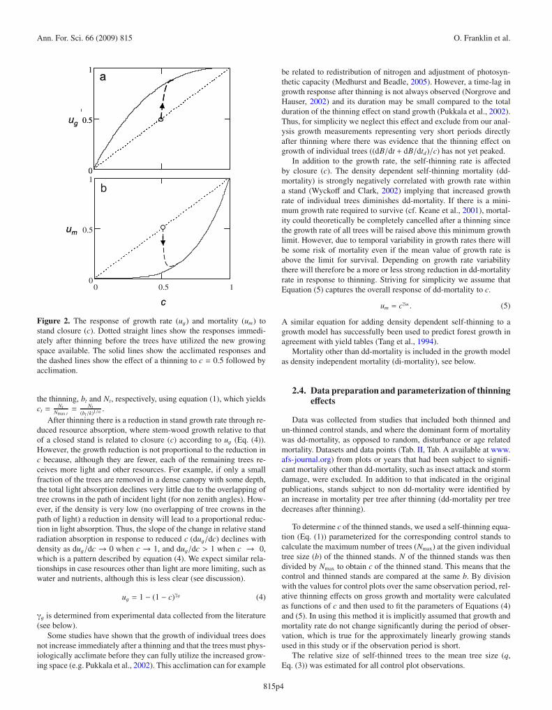
Figure 2. The response of growth rate (ug) and mortality (um) tostand closure (c). Dotted straight lines show the responses immedi-ately after thinning before the trees have utilized the new growingspace available. The solid lines show the acclimated responses andthe dashed lines show the effect of a thinning to c = 0.5 followed byacclimation.
the thinning, bt and Nt, respectively, using equation (1), which yieldsct =
NtNmax t
= Nt
(bt/k)1/α.
After thinning there is a reduction in stand growth rate through re-duced resource absorption, where stem-wood growth relative to thatof a closed stand is related to closure (c) according to ug (Eq. (4)).However, the growth reduction is not proportional to the reduction inc because, although they are fewer, each of the remaining trees re-ceives more light and other resources. For example, if only a smallfraction of the trees are removed in a dense canopy with some depth,the total light absorption declines very little due to the overlapping oftree crowns in the path of incident light (for non zenith angles). How-ever, if the density is very low (no overlapping of tree crowns in thepath of light) a reduction in density will lead to a proportional reduc-tion in light absorption. Thus, the slope of the change in relative standradiation absorption in response to reduced c (dug/dc) declines withdensity as dug/dc → 0 when c → 1, and dug/dc > 1 when c → 0,which is a pattern described by equation (4). We expect similar rela-tionships in case resources other than light are more limiting, such aswater and nutrients, although this is less clear (see discussion).
ug = 1 − (1 − c)γg (4)
γg is determined from experimental data collected from the literature(see below).
Some studies have shown that the growth of individual trees doesnot increase immediately after a thinning and that the trees must phys-iologically acclimate before they can fully utilize the increased grow-ing space (e.g. Pukkala et al., 2002). This acclimation can for example
be related to redistribution of nitrogen and adjustment of photosyn-thetic capacity (Medhurst and Beadle, 2005). However, a time-lag ingrowth response after thinning is not always observed (Norgrove andHauser, 2002) and its duration may be small compared to the totalduration of the thinning effect on stand growth (Pukkala et al., 2002).Thus, for simplicity we neglect this effect and exclude from our anal-ysis growth measurements representing very short periods directlyafter thinning where there was evidence that the thinning effect ongrowth of individual trees ((dB/dt + dB/dtd)/c) has not yet peaked.
In addition to the growth rate, the self-thinning rate is affectedby closure (c). The density dependent self-thinning mortality (dd-mortality) is strongly negatively correlated with growth rate withina stand (Wyckoff and Clark, 2002) implying that increased growthrate of individual trees diminishes dd-mortality. If there is a mini-mum growth rate required to survive (cf. Keane et al., 2001), mortal-ity could theoretically be completely cancelled after a thinning sincethe growth rate of all trees will be raised above this minimum growthlimit. However, due to temporal variability in growth rates there willbe some risk of mortality even if the mean value of growth rate isabove the limit for survival. Depending on growth rate variabilitythere will therefore be a more or less strong reduction in dd-mortalityrate in response to thinning. Striving for simplicity we assume thatEquation (5) captures the overall response of dd-mortality to c.
um = cγm . (5)
A similar equation for adding density dependent self-thinning to agrowth model has successfully been used to predict forest growth inagreement with yield tables (Tang et al., 1994).
Mortality other than dd-mortality is included in the growth modelas density independent mortality (di-mortality), see below.
2.4. Data preparation and parameterization of thinningeffects
Data was collected from studies that included both thinned andun-thinned control stands, and where the dominant form of mortalitywas dd-mortality, as opposed to random, disturbance or age relatedmortality. Datasets and data points (Tab. II, Tab. A available at www.afs-journal.org) from plots or years that had been subject to signifi-cant mortality other than dd-mortality, such as insect attack and stormdamage, were excluded. In addition to that indicated in the originalpublications, stands subject to non dd-mortality were identified byan increase in mortality per tree after thinning (dd-mortality per treedecreases after thinning).
To determine c of the thinned stands, we used a self-thinning equa-tion (Eq. (1)) parameterized for the corresponding control stands tocalculate the maximum number of trees (Nmax) at the given individualtree size (b) of the thinned stands. N of the thinned stands was thendivided by Nmax to obtain c of the thinned stand. This means that thecontrol and thinned stands are compared at the same b. By divisionwith the values for control plots over the same observation period, rel-ative thinning effects on gross growth and mortality were calculatedas functions of c and then used to fit the parameters of Equations (4)and (5). In using this method it is implicitly assumed that growth andmortality rate do not change significantly during the period of obser-vation, which is true for the approximately linearly growing standsused in this study or if the observation period is short.
The relative size of self-thinned trees to the mean tree size (q,Eq. (3)) was estimated for all control plot observations.
All values are means for each species. 1 Number of observations, 2 mean stand age during experiment, 3 duration over which mean responses wereestimated, 4 adjusted value, measured value was 1.27. References for studies 1–5, respectively: Johnstone (2002), Montero et al. (2001), Omule (1988),Watanabe (2002), Asai (1997). The complete data set is shown in Appendix Table.
0 200 400 6000
100
200
300
B
N
N0
N1
N2
0 1 2 30.4
0.6
0.8
B/B0
c
c1
c2
0 200 400 6000
100
200
300
B
N
N0
N1
N2
0 200 400 6000
100
200
300
B
N
N0
N1
N2
0 1 2 30.4
0.6
0.8
B/B0
c
0 1 2 30.4
0.6
0.8
B/B0
c
c1
c2
Figure 3. Development of tree numbers (N) and closure (c) after thinning of a closed stand (B = B0, N = N0, c = 1) at two levels of biomassremoval, 25% (N1, c1 dashed lines) and 50% (N2, c2 dotted lines). Parameter values: k = 3000, γm = 4, α = −1.5.
2.5. Growth and mortality dynamics of thinned stands
For net increment (dB/dt) the total effect of a thinning dependson the relative strength of the effects on stand growth and mortality.For a moderate thinning, the avoided self-thinning usually more thancompensates for the reduction in total stand production so that netstem increment is enhanced. After a thinning, the c of the thinnedstand increases with time and may eventually approach a fully closedstand (c = 1; Fig. 3).
In a closed stand, net increment (dB/dtc) and mortality (dBd/dtc)are linked according to equation (3). In a thinned (open) stand, totalstem wood production is reduced according to equation (4) and selfthinning (second term in Eq. (6)) is reduced according to equation (5)as functions of closure (c)
dBdt=
(dBdtc+
dBd
dtc
)ug − dBd
dtcum. (6)
As this study focuses on the analysis of managed stands where den-sity independent mortality is low, density independent mortality isignored in equation (6). However for other applications and for ourillustrated scenario below, density independent mortality is added tothe framework. By definition density independent mortality (dBdi/dt,Eq. (7)) does not change as a function of c. For spruce stands mor-tality has been shown to be higher for very small and very big trees(Monserud and Sterba, 1999), i.e. slow growing stages (in terms of
absolute growth rate) of stand development, and is therefore modeledto be a function of the net increment (dB/dt) relative to its maximumover the stand development (dB/dtmax)
dBdtdi= mB
(1 − dB/dt
dB/dtmax
). (7)
Because of its independence of c, density independent mortality inthis study only plays a role in the illustration of thinning scenariosbelow, where m was assumed to be 1% per year.
Using equations (1)–(6), the stand behavior in terms of biomass(B) and mortality (Bd) can be derived as functions of closure (c) andtime for thinned stands.
The relationship between c, N and B can also be described inde-pendently of time and dB/dt using equations (1), (3), (5) and (6). Toillustrate their behavior, we derive analytical expressions for the de-velopment of c and N after a thinning removal of a fraction ft of thestanding biomass just before thinning (B0), as functions of B devel-opment after the thinning:
c =
⎡⎢⎢⎢⎢⎢⎢⎢⎢⎣1 −(
BB0
11 − ft
) γmα (
1 − (c0 (1 − ft))−γm)
⎤⎥⎥⎥⎥⎥⎥⎥⎥⎦−1/γm
(8)
N =
⎡⎢⎢⎢⎢⎢⎢⎣(k/B)γm/α +
(k(1 − ft)−(a+1)
B0c0
)γm/α−
(k
B0(1 − ft)
)γm/α⎤⎥⎥⎥⎥⎥⎥⎦−α/(γm(α+1))
.
(9)
815p5
Ann. For. Sci. 66 (2009) 815 O. Franklin et al.
In case the mean size of the trees removed in a thinning is not equalto the mean tree size of the stand, B0 in Equations (8) and (9) must berecalculated to match b after thinning (bt, Fig. 1).
The behavior of N and c after a thinning (Eqs. (8) and (9)) is il-lustrated in Figure 3. The development of c and N after a thinning ofa closed stand depend on the fraction biomass removed in the thin-ning ( ft), the maximum N as a function of B (the self thinning equa-tion, Eq. (1)) and the density response of self thinning mortality (γm,Eq. (5)).
Because the Equations (4)–(9) above are independent of the func-tional form of the basic increment function (dB/dtc), the frameworkcan be used to describe the thinning response in combination with anybasic growth function. In summary, the parameters that are needed toadd a thinning response to any growth model of standing biomass (B)are the parameters of the self thinning equation k, and α, the growthand mortality response parameters γg and γm, and the closure beforethinning, c0. To obtain a time dependent response (as opposed to onlyB dependent) it is also necessary to know the relative size of self-thinning compared to surviving trees (q), see below.
2.6. Optimal closure and thinning
To determine the optimal c in terms of net stem biomass incre-ment we consider net increment dB/dt (Eq. (6)) as c is reduced. Netincrement is decreased due to reduced gross growth at the same timeas it is increased due to reduced self thinning mortality (Fig. 2). Themaximum net increment is obtained where the sum of the two effectson dB/dt (Eq. (6)) is maximized. Using Equation (3), Equation (6)can be reformulated as
dBdt=
(dBdtc+
dBdtc
qα + 1
)ug − dB
dtc
qα + 1
um =
dBdtc
(( qα + 1
+ 1)
ug − qα + 1
um
)(10)
dB/dt is maximized by setting Equation (10) = 0, inserting the func-tions for um and ug (Eqs. (4) and (5)) and solving for c,
ddc
(( qα + 1
+ 1)
ug − qα + 1
um
)= γg
(1 +
qα + 1
)(1 − c)γg−1
− γmqα + 1
cγm−1 = 0. (11)
To obtain the optimal c, Equation (11) must be solved numerically.A sensitivity analysis of optimal c was conducted with regard to
the density effects on mortality (γm) and growth (γg) and relative sizeof self-thinned trees (q). Net increment gain in a thinned stand wasanalyzed in comparison to un-thinned (c = 1) stands.
The equations above illustrate the responses of a forest stand toa specified thinning. To describe the development of a forest standmanaged by successive thinnings and calculate an optimal thinninglevel in terms of maximized biomass increment, it is also necessaryto describe how and when thinnings are initiated.
In order to illustrate an example of an optimal thinning scenariobased on our model and the optimal c, a thinning scenario was de-signed to keep c within a near-optimal range. We base our thinningscenario on the assumption that the purpose of the thinning is to en-hance biomass productivity. In addition, although we do not explicitlyconsider any economical factors, the thinning scenario should not beunrealistic in relation to practical applications that include manage-ment costs and benefits. The number of thinnings should not be too
0.0 0.2 0.4 0.6 0.8 1.00.0
0.2
0.4
0.6
0.8
1.0
1.2
1.4 a
c0.0 0.2 0.4 0.6 0.8 1.0
0.0
0.2
0.4
0.6
0.8
1.0
1.2
1.4
Gold birchMonarch birch
Scots pineHemlock
Lodgepole pineb
Rel
ativ
e gr
oss
incr
emen
t (u g
)R
elat
ive
mor
talit
y (um)
0.0 0.2 0.4 0.6 0.8 1.00.0
0.2
0.4
0.6
0.8
1.0
1.2
1.4 a
c0.0 0.2 0.4 0.6 0.8 1.0
0.0
0.2
0.4
0.6
0.8
1.0
1.2
1.4
Gold birchMonarch birch
Scots pineHemlock
Lodgepole pineb
Rel
ativ
e gr
oss
incr
emen
t (u g
)R
elat
ive
mor
talit
y (um)
Figure 4. Relative gross stem-wood increment (a) and mortality (b)as functions of closure (c). Solid lined are best fits for all speciespooled (see Tab. II). One point for Scots pine was outside of the plot-ted range (relative mortality = 2.14, c = 0.95).
high, since very frequent thinnings would be cost-intensive. Further-more we presume that no thinning occurs before the stand has reacheda certain biomass and tree size because very early thinnings wouldyield relatively little harvest of thin stems (low value) at the sametime as costs are high due to the large number of stems that need tobe cut. The point of first thinning also depends on the planting density(for planted stands) as the stand must have a sufficiently high closure(c) before thinning is beneficial (see below). We set the timing of thefirst thinning equal to the point of peak growth, which in forest standsimulations with realistic planting densities (much lower than maxi-mum density (Nmax), i.e. c � 1) nearly coincided with c reaching thecomputed limit for optimal thinning (c ≈ 0.85).
3. RESULTS
3.1. Density effects on growth and mortality
Table III and Figure 4 show the fitted parameters and thedata for relative growth and mortality as functions of c for dif-ferent species and for all species pooled. There are statisticallysignificant differences in γg (p = 0.0004) and γm (p = 0.044)among species although the number of data points is smalland confidence intervals are large for most species. Residualanalysis showed that the c effect on gross increment is rea-sonably well described by equation (4) with a r2 = 0.41 forall species pooled, and with higher r2 for the species specificfits (Tab. III). For mortality, the agreement between model and
815p6
Model of thinning effects Ann. For. Sci. 66 (2009) 815
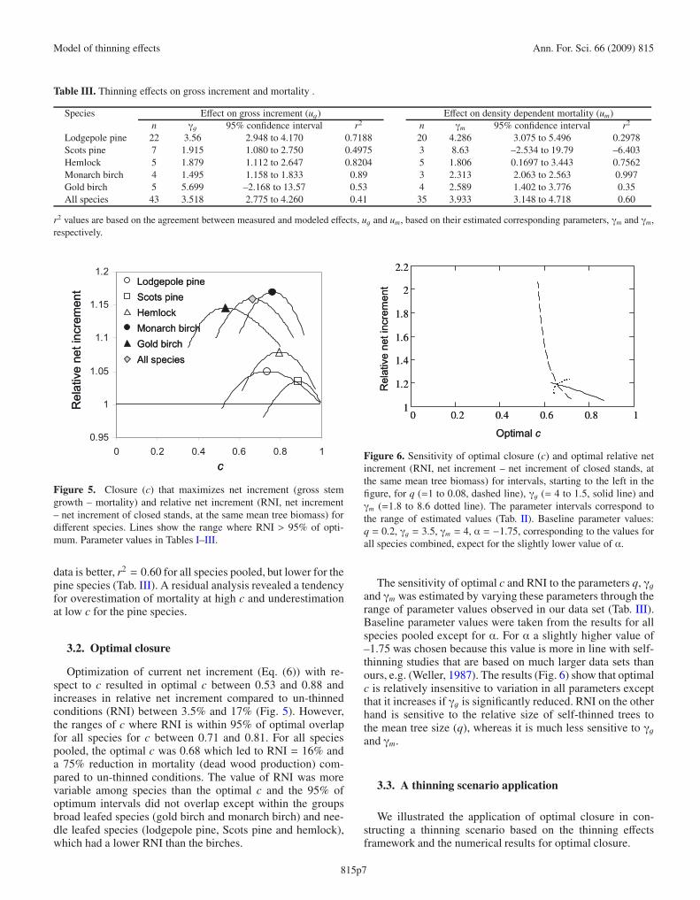
Table III. Thinning effects on gross increment and mortality .
Species Effect on gross increment (ug) Effect on density dependent mortality (um)n γg 95% confidence interval r2 n γm 95% confidence interval r2
Lodgepole pine 22 3.56 2.948 to 4.170 0.7188 20 4.286 3.075 to 5.496 0.2978Scots pine 7 1.915 1.080 to 2.750 0.4975 3 8.63 –2.534 to 19.79 –6.403Hemlock 5 1.879 1.112 to 2.647 0.8204 5 1.806 0.1697 to 3.443 0.7562Monarch birch 4 1.495 1.158 to 1.833 0.89 3 2.313 2.063 to 2.563 0.997Gold birch 5 5.699 –2.168 to 13.57 0.53 4 2.589 1.402 to 3.776 0.35All species 43 3.518 2.775 to 4.260 0.41 35 3.933 3.148 to 4.718 0.60
r2 values are based on the agreement between measured and modeled effects, ug and um, based on their estimated corresponding parameters, γm and γm,respectively.
0.95
1
1.05
1.1
1.15
1.2
0 0.2 0.4 0.6 0.8 1
Lodgepole pineScots pineHemlockMonarch birchGold birchAll species
c
Rel
ativ
e ne
t inc
rem
ent
0.95
1
1.05
1.1
1.15
1.2
0 0.2 0.4 0.6 0.8 1
Lodgepole pineScots pineHemlockMonarch birchGold birchAll species
Lodgepole pineScots pineHemlockMonarch birchGold birchAll species
c
Rel
ativ
e ne
t inc
rem
ent
Figure 5. Closure (c) that maximizes net increment (gross stemgrowth – mortality) and relative net increment (RNI, net increment– net increment of closed stands, at the same mean tree biomass) fordifferent species. Lines show the range where RNI > 95% of opti-mum. Parameter values in Tables I–III.
data is better, r2 = 0.60 for all species pooled, but lower for thepine species (Tab. III). A residual analysis revealed a tendencyfor overestimation of mortality at high c and underestimationat low c for the pine species.
3.2. Optimal closure
Optimization of current net increment (Eq. (6)) with re-spect to c resulted in optimal c between 0.53 and 0.88 andincreases in relative net increment compared to un-thinnedconditions (RNI) between 3.5% and 17% (Fig. 5). However,the ranges of c where RNI is within 95% of optimal overlapfor all species for c between 0.71 and 0.81. For all speciespooled, the optimal c was 0.68 which led to RNI = 16% anda 75% reduction in mortality (dead wood production) com-pared to un-thinned conditions. The value of RNI was morevariable among species than the optimal c and the 95% ofoptimum intervals did not overlap except within the groupsbroad leafed species (gold birch and monarch birch) and nee-dle leafed species (lodgepole pine, Scots pine and hemlock),which had a lower RNI than the birches.
Optimal c
Rel
ativ
e ne
t inc
rem
ent
0 0.2 0.4 0.6 0.8 11
1.2
1.4
1.6
1.8
2
2.2
Optimal c
Rel
ativ
e ne
t inc
rem
ent
0 0.2 0.4 0.6 0.8 11
1.2
1.4
1.6
1.8
2
2.2
Figure 6. Sensitivity of optimal closure (c) and optimal relative netincrement (RNI, net increment – net increment of closed stands, atthe same mean tree biomass) for intervals, starting to the left in thefigure, for q (=1 to 0.08, dashed line), γg (= 4 to 1.5, solid line) andγm (=1.8 to 8.6 dotted line). The parameter intervals correspond tothe range of estimated values (Tab. II). Baseline parameter values:q = 0.2, γg = 3.5, γm = 4, α = −1.75, corresponding to the values forall species combined, expect for the slightly lower value of α.
The sensitivity of optimal c and RNI to the parameters q, γgand γm was estimated by varying these parameters through therange of parameter values observed in our data set (Tab. III).Baseline parameter values were taken from the results for allspecies pooled except for α. For α a slightly higher value of–1.75 was chosen because this value is more in line with self-thinning studies that are based on much larger data sets thanours, e.g. (Weller, 1987). The results (Fig. 6) show that optimalc is relatively insensitive to variation in all parameters exceptthat it increases if γg is significantly reduced. RNI on the otherhand is sensitive to the relative size of self-thinned trees tothe mean tree size (q), whereas it is much less sensitive to γgand γm.
3.3. A thinning scenario application
We illustrated the application of optimal closure in con-structing a thinning scenario based on the thinning effectsframework and the numerical results for optimal closure.
815p7
Ann. For. Sci. 66 (2009) 815 O. Franklin et al.
To maximize current net increment in a thinning scenario, cshould be kept as near the optimum as possible. In theory thiscould be achieved by frequent thinnings that never allow thestand to deviate from the optimal c. In practice, thinnings areassociated with costs and a very frequent thinning regime isnot realistic. However, the peak of net increment as a functionof c is not particularly steep (Fig. 5), which means that somevariation around the optimal density, for example between 0.5and 0.9, does not severely reduce net increment (≈5% reduc-tion compared to optimal c, for the pooled species parametervalues; Fig. 5). At the same time, the frequency of thinningscan be significantly reduced compared to a narrower intervalof allowed c values.
Based on the above results, a thinning scenario is outlinedas follows. After peak growth rate has been reached, the firstthinning is performed according to a specified level ( ft, frac-tion stem biomass removed). After the thinning the relativedensity of the stand (c) will increase and eventually approacha closed stand (Fig. 3). The next thinning is triggered when thestand has reached a specified c = ct. Thereafter, new thinningsare triggered each time c reaches ct. Thus, a thinning scenariois specified by the B at initial thinning (at maximum growthrate), the fraction stem biomass removed ( ft) and the value ofc that triggers a new thinning (ct). Figure 7 illustrates a thin-ning scenario compared to an un-thinned stand. In practice, itis however necessary to consider the development stage andthe timing of final harvest before a thinning is done.
4. DISCUSSION
4.1. General assumptions
Our aim was to develop a model of thinning effects generalenough to be applied to any even-aged forest stand and yetsimple enough to be used without re-formulation for all forestsin temperate or boreal regions. For this reason the model wasbased on the concept of closure (c), i.e. the stand density rela-tive to maximum stand density and relative rates of growth andmortality, i.e. growth and mortality relative to a stand at maxi-mum density (c = 1). Although a conceptually very similar ap-proach has been presented before (Pretzsch, 2005), time basedapproaches are far more common. Commonly, effects of dif-ferent densities after thinning are compared at the same pointsin time, which means that the responses will be strongly timedependent due to the closing of the stand over time and the dif-fering growth rates at different densities. In contrast, our use ofc, the density compared to maximum density at the same meantree biomass (b), provides an invariable basis for evaluatingdensity effects measured over different time spans. This modelimplies that site conditions affect only the rate of change butnot the path of relative density and biomass development of astand, which has ample empirical support (Long et al., 2004).
In using c as the single control of density effects, indepen-dent of age or tree size, we implicitly assume that competi-tion among trees and stand size structure qualitatively doesnot change significantly during stand development. Stabilityof size structure and competitive interactions in self-thinning
0 20 40 60 80 100 120 140 160
YD
ata
0
1
2
3
4
0
50
100
150
200
250
300
0
500
1000
1500
2000
2500
3000
3500
Bio
mas
s (M
g ha
-1)
Tree
num
bers
( ha
-1)
Net
incr
emen
t (M
g ha
-1y-1
)
years
A
B
C
0 20 40 60 80 100 120 140 160
YD
ata
0
1
2
3
4
0
50
100
150
200
250
300
0
500
1000
1500
2000
2500
3000
3500
-1)
-1)
Net
incr
emen
t (M
g ha
-1y-1
)
years
A
B
C
Figure 7. Examples of the development of un-thinned (solid line)and a thinned stand (dashed line) simulated with a forest growthmodel for un-thinned stands (Franklin et al., 2009) combined with thethinning scenario presented here, including the effect of competitionun-related mortality (Eq. (7)). Thinnings that reduce closure (c) toc = 0.6 are triggered when c > 0.85. The stand is Scots pine plantedat 3000 trees per ha. Net increment (C) is gross biomass growth –mortality.
stands of plants has been shown to result from asymmetriccompetition (larger trees affecting smaller trees much morethan the other way around) (Hara, 1993). For older stands therole of competition may, however, change, leading to changesin size distributions (Coomes and Allen, 2007). Although thisstudy does not include old-growth stands, equation (7) showshow the effect of reduced competition and relatively increaseddensity independent mortality in older stands can be includedin our model. A change in size distribution may also affectthe relative size difference between self-thinned and surviving
815p8
Model of thinning effects Ann. For. Sci. 66 (2009) 815
trees (q), which would violate our assumption of constant q.For the two studies with more than one record of q there wasa clear increase over time for Scots pine (average +64% over10 y) but not for lodgepole pine (+3.8% over 10 y). The in-crease in q for Scots pine coincides with a reduction in incre-ment of 32%, which did not occur in the Lodgepole pine stand,and indicates that net growth rate of the Scots pine stand haspassed its peak and is declining. Such aging of stands is asso-ciated with changes in size distribution and an increase in den-sity independent mortality, as discussed above. Thus, densityindependent mortality of larger trees may explain the apparentincrease in q for Scots pine.
Because competition related mortality risk is strongly nega-tively correlated with individual tree growth rate within a stand(Wyckoff and Clark, 2002) one may expect that it is possi-ble to make our mortality effect (um) a function of the effecton growth (ug) and thereby simplify the model. However, wedid not find any correlation between individual growth (ug/c)and mortality risk (um/c) in response to stand closure amongspecies. This result indicates that mortality risk is affected byother factors in addition to growth rate. For example, becausemortality in contrast to growth is a threshold event for the indi-vidual, it could respond stronger to environmental variabilitythan growth. Even if the mean resource availability and cli-mate conditions over time are sufficient for survival, temporalfluctuations could cause mortality. Furthermore, it has beenshown that while growth is closely linked to stand density,an additional density measure, gap fraction, affects mortality(Zeide, 2005). Clearly, our separate effects of density (c) onmortality (um) and growth (ug) cannot be uniquely combinedto a common density effect, at least not without introducinga more complex density measure, which, however, would notbe compatible with our aim of parsimony in order to facilitatewide applicability of the model.
It is implicit in our model that gross increment is maxi-mized at c = 1, which has been showed in previous studiesof optimal density (Zeide, 2004). However, Zeide (2004) didnot explicitly include mortality and did not find a simple rela-tionship for optimal net increment due to interacting effects ofstand density and b. In contrast, by our comparison of c valuesat a common b we avoid this interaction of effects and obtainan expression for optimal net increment as a trade-off betweenexplicit mortality and growth effects.
4.2. Optimal closure
The estimated ranges of near optimum (> 95% of maxi-mum) c in Figure 5 show that these ranges overlap for allspecies between c = 0.71 to c = 0.81, indicating that a caround 0.75 may, in our framework, be generally applicablefor optimal thinning (to maximize net increment) for mostspecies. The range of near optimal c for all species pooledc = 0.5 to 0.9 is in general agreement with the results of thin-ning trials of (Assmann, 1961), reporting relative stand densi-ties (basal area) between 0.6 and 0.9 as threshold for achievingoptimum stem productivity. The sensitivity analysis indicatedthat optimal c is quite robust with respect to variation in pa-
rameter values although it is slightly increased with decreasingclosure effect on growth (γg), which acts to reduce the positiveresponse of growth of remaining trees after a thinning (Fig. 6).
In comparison to optimal c, the maximum relative gain innet increment (RNI) is more variable among species, althoughthe range of 4 to 16% is rather limited (Fig. 5). RNI is alsomore sensitive than optimal c to parameter changes, particu-larly to the size ratio of self-thinning trees to the mean tree, q(Fig. 6). The reason for the model sensitivity to q is that thisparameter determines the mortality rate (dead wood produc-tion) relative to net increment and thereby controls how muchmortality can be avoided (and added to net increment) by thin-ning. Our data showed a variation in q between 0.06 and 1.27,where the latter value (Monarch birch) was considered unreal-istic and was therefore set to 1. Such a high estimate of q mayindicate that the mortality was not due to competition and self-thinning and therefore not representative, as discussed above.If Monarch birch is excluded, our range of q is between 0.06and 0.321. For additional assessment of q variability, a simu-lation experiment was conducted with the hybrid patch modelPICUS v1.4 (Seidl et al., 2005) that models mortality at theindividual tree level. Starting from generic homogeneous ini-tial stand conditions 100 y simulations over an array of speciesand environmental conditions (cf. Seidl et al., 2009) resultedin values of q between 0.5 and 0.25.
Comparing species specific results, model results for Scotspine, both in terms of optimal c (= 0.9) and the low in-crease in net increment in thinned compared to closed stands(RNI = 4%) is in agreement with results by Mäkinen andIsomäki (2004). For lodgepole pine our result for the grossand net increment as a function of c are in reasonable agree-ment with the findings of Cochran and Dahms (2000). Ourmodel study suggests that the potential increase in RNI maybe higher for the deciduous broad-leafed species than for theneedle leafed species (Fig. 5), which was previously observedwhen comparing beech (RNI ≈ 20%) and spruce (RNI ≈ 10%)(Pretzsch, 2005). Although there were significant differencesin the closure effects on growth and mortality, γg and γm,among species, these differences could be misleading becausethey could also be related to site differences. There are also dif-ferences in the self-thinning parameter α and the relative sizeof self-thinned trees (q) among the species but more data isclearly needed to obtain confident conclusions about speciesor site effects. However, the requirement that data must in-clude both increment and mortality in terms of both numbersand biomass (or volume) substantially limits the availability ofsuitable data.
An potential factor of uncertainty in the estimation of stem-wood productivity gain of thinning is related to the potentialdelay in growth response after a thinning due to a phase ofphysiological acclimation as discussed above (Materials andmethods –thinning effects). Such an effect would reduce thepotential gain of a thinning but would not affect the optimal c.The delay could significantly affect the optimal frequency ofthinnings if the phase of acclimation covers a significant pro-portion of the growing time, which, however, was not found inthe experiments analyzed in our study.
815p9
Ann. For. Sci. 66 (2009) 815 O. Franklin et al.
4.3. Limitations and potential extensions
An approach based on self-thinning as a function of meantree size does not adequately represent strongly age- hetero-geneous stands and is not applicable to management systemssuch as continuous cover forestry or variable retention sys-tems, which are increasingly discussed as alternatives to even-aged management strategies (cf. Seidl et al., 2008).
Due to limited data availability, our model does not includeeffects of site conditions on the thinning response. This is aclear limitation of the model as several studies point at con-siderably varying responses with local site conditions (e.g.,Pretzsch, 2005). Underlying these empirical observations are,however, complex interactions of environmental and physio-logical factors, such as soil fertility, soil depth, water availabil-ity, climate and disturbance. These interactions are rarely rep-resented at the data resolution available at continental scalesand they are quantitatively not well understood in terms ofgeneral relationships valid across species and environmentalconditions, which prevent their inclusion in our model. Inter-actions among resource availability, climate and density rela-tionships remain an interesting topic for further research andpotential development of more detailed models.
Considering that a main aspect of thinning, besides focus-ing growth on the remaining individuals, is to improve standstability and quality, neglecting these aspects in taking a meantree approach might represent another limitation of the pre-sented model. While generic effects on the stand collectivecan be mimicked by means of the relative size of removedtrees (e.g., thinning from above, thinning from below – seeFig. 1) the approach lacks the flexibility of individual-treemodels with regard to spatially heterogeneous and selectiveapproaches (cf. Hasenauer, 2006) Furthermore, although weconsider thinning-related biomass (or volumetric) changes ofthe mean tree in our model, allocational shifts in stem allome-try between e.g., height and diameter increment are not explic-itly included. A simple way to obtain the effects on diametergrowth would be to assume that mean tree height is not af-fected by thinning (e.g. Cochran and Dahms, 2000) and useallometric functions to derive the effects on diameter directlyfrom biomass results.
Overall, considering that model complexity is strongly de-termined by the intended domain of application we believe thatthe presented approach is a reasonable compromise betweenecological realism and general, large-scale applicability.
4.4. Conclusions for model applicability
For prognostic modeling our use of relative, site- andproductivity-independent changes in gross growth (ug) andmortality (um) allows integration with any existing forest in-crement model for un-thinned stands. In combination withequations for tree numbers (Eq. (8)) and closure (Eq. (9)),stand development in terms of biomass, dead wood and asso-ciated tree numbers can be obtained for an arbitrary thinningscenario. The simplicity of the approach makes it potentiallyuseful for large scale, continental and global modeling of net
increment and mortality where site information is limited ornon-existing, or where computation time (e.g. in dynamic op-timization frameworks) or ease of mathematical integration isan issue. For example, the approach could add realism to largescale policy related analyses (e.g. Böttcher et al., 2008) or foranalyses using global dynamic vegetation models (e.g. Zaehleet al., 2006).
The presented framework is an attempt to transfer the de-tailed accumulated knowledge on thinning responses repre-sented in detailed growth and yield models (e.g., overviewsin Hasenauer, 2006; Söderbergh and Ledermann, 2003) andthinning experiments to model frameworks at larger spatialscales in a general and physiologically meaningful set of equa-tions. This approach necessarily sacrifices complexity anddetails compared to comprehensive individual-based models(Crookston and Dixon, 2005; Hyytiäinen et al., 2004; Sterbaand Monserud, 1997). However, the selected mean tree ap-proach is a structural advancement of the state of the artcompared to structurally simple scenario tools applied at con-tinental scale (e.g. Schelhaas et al., 2007). In conclusion, in-troducing a generic thinning framework as presented in thisstudy in large scale scenario analyses of forest resource devel-opment could significantly increase their realism with regardto the silvicultural decision space in forest management.
Acknowledgements: We thank Hannes Böttcher at IIASA for help-ful comments on the manuscript. We are furthermore grateful to twoanonymous reviewers for helping to improve an earlier version of themanuscript. This research received funding from the European Com-munity’s 7th Framework Programme (FP7) under the grant 212535,Climate Change - Terrestrial Adaptation and Mitigation in Europe(CC-TAME), www.cctame.eu, and from the 6th Framework Pro-gramme (FP6) under the grant SSPI551 CT-2003/503614 (INSEA).
REFERENCES
Asai T., 1997. Effect of varying thinning densities on tree growth in aJapanese birch forest. Hokkaido Branch Journal of Japanese ForestResearch 45: 50–52.
Assmann F., 1961. Waldertragskunde. Organische Produktion, Struktur,Zuwachs und Ertrag von Waldbeständen. BLV Verlagsgesellschaft,München, 490 p.
Böttcher H., Freibauer A., Obersteiner M., and Schulze E.D., 2008.Uncertainty analysis of climate change mitigation options in theforestry sector using a generic carbon budget model. Ecol. Model.213: 45–62.
Cochran P.H. and Dahms W.G., 2000. Growth of lodgepole pine thinnedto various densities on two sites with differing productivities incentral Oregon. USDA Forest Service, Research Papers RMRS,pp. 1–59.
Coomes D.A. and Allen R.B., 2007. Mortality and tree-size distributionsin natural mixed-age forests. J. Ecol. 95: 27–40.
Crookston N.L. and Dixon G.E., 2005. The forest vegetation simulator: Areview of its structure, content, and applications. Comput. Electron.Agric. 49: 60–80.
Dewar R.C. and Porte A., 2008. Statistical mechanics unifies differentecological patterns. J. Theor. Biol. 251: 389–403.
Franklin O., Moltchanova E., Obersteiner M., Kraxner F., Seidl R.,Böttcher H., and Rokityianskiy D., 2009. A European scale forestgrowth and thinning model-deducing productivity and stand densityfrom inventory data manuscript.
815p10
Model of thinning effects Ann. For. Sci. 66 (2009) 815
Garcia O., 1990. Growth of Thinned and Pruned Stands. In New ap-proaches to spacing and thinning in plantation forestry. Proceedingsof a IUFRO symposium, Rotorua, New Zealand, April 1989, JamesR.N., Tarlton G.L. (Eds.)., New Zealand Ministry of Forestry, ForestResearch Institute.
Hara T., 1993. Model of competition and size-structure dynamics in plantcommunities. Plant Species Biol. 8: 75–84.
Hasenauer H., 2006. Concepts within tree growth modeling. In:Hasenauer H. (Ed.), Sustainable Forest Management. GrowthModels for Europe, Berlin, pp. 3–17.
Hynynen J., Ahtikoski A., Siitonen J., Sievänen R., and Liski J., 2005.Applying the MOTTI simulator to analyse the effects of alternativemanagement schedules on timber and non-timber production. For.Ecol. Manage. 207: 5–18.
Hyytiäinen K., Hari P., Kokkila T., Maäkela A., Tahvonen O., and TaipaleJ., 2004. Connecting a process-based forest growth model to stand-level economic optimization. Can. J. For. Res. 34: 2060–2073.
Johnstone W.D., 2002. Thinning Lodgepole Pine in Southeastern BritishColumbia: 46-year Results. Res. Br., B.C. Min. For., Victoria, B.C.,Work. Pap. 63.
Keane R.E., Austin M., Field C., Huth A., Lexer M.J., Peters D., SolomonA., et al., 2001. Tree mortality in gap models: Application to climatechange. Clim. Change 51: 509–540.
Kurz W.A. and Apps M.J., 1999. A 70-year retrospective analysis of car-bon fluxes in the Canadian Forest Sector. Ecol. Appl. 9: 526–547.
Long J.N., Dean T.J., and Roberts S.D., 2004. Linkages between silvi-culture and ecology: Examination of several important conceptualmodels. For. Ecol. Manage. 200: 249–261.
Mäkinen H. and Isomäki A., 2004. Thinning intensity and growth of Scotspine stands in Finland. For. Ecol. Manage. 201: 311–325.
Mason E.G. and Dzierzon H., 2006. Applications of modeling to vegeta-tion management. Can. J. For. Res. 36: 2505–2514.
Medhurst J.L. and Beadle C.L., 2005. Photosynthetic capacity and foliarnitrogen distribution in Eucalyptus nitens is altered by high-intensitythinning. Tree Physiol. 25: 981–991.
Monserud R.A. and Sterba H., 1999. Modeling individual tree mortalityfor Austrian forest species. For. Ecol. Manage. 113: 109–123.
Montero G., Canellas I., Ortega C., and Del Rio M., 2001. Results froma thinning experiment in a Scots pine (Pinus sylvestris L.) naturalregeneration stand in the Sistema Iberico Mountain Range (Spain).For. Ecol. Manage. 145: 151–161.
Newnham R.M., 1964. The development of a stand model for Douglasfir. Ph.D. thesis, University of British Columbia, Vancouver, 201 p.
Norgrove L. and Hauser S., 2002. Measured growth and tree biomass esti-mates of Terminalia ivorensis in the 3 years after thinning to differentstand densities in an agrisilvicultural system in southern Cameroon.For. Ecol. Manage. 166: 261–270.
Omule S.A.Y., 1988. Growth and yield 35 years after commercially thin-ning 50-year-old Douglas-fir. Can. For. Serv. and B.C. Min. For.,Victoria, B.C., FRDA Rep. 021: 7.
Petritsch R., Hasenauer H., and Pietsch S.A., 2007. Incorporating forestgrowth response to thinning within biome-BGC. For. Ecol. Manage.242: 324–336.
Pretzsch H., 2005. Stand density and growth of Norway spruce(Picea abies (L.) Karst.) and European beech (Fagus sylvatica L.):Evidence from long-term experimental plots. Eur. J. For. Res. 124:193–205.
Pukkala T., Miina J., and Palahi M., 2002. Thinning response and thin-ning bias in a young Scots pine stand. Silva Fenn. 36: 827–840.
Reineke L.H., 1933. Perfecting a stand-density index for even-agedforests. J. Agric. Res. 46: 627–638.
Schelhaas M.J., Eggers J., Lindner M., Nabuurs G.J., Pussinen A.,Päivinen R., Schuck A., et al., 2007. Model documentation for theEuropean Forest Information Scenario model (EFISCEN 3.1.3), EFITechnical Report.
Seidl R., Lexer M.J., Jäger D., and Hönninger K., 2005. Evaluating theaccuracy and generality of a hybrid patch model. Tree Physiol. 25:939–951.
Seidl R., Rammer W., Lasch P., Badeck F.W., and Lexer M.J., 2008.Does conversion of even-aged, secondary coniferous forests affectcarbon sequestration? A simulation study under changing environ-mental conditions. Silva Fenn. 42: 369–386.
Seidl R., Rammer W., and Lexer M., 2009. Schätzung vonBodenmerkmalen und Modellparametern für die Waldökosystem-simulation auf Basis einer Großrauminventur. Allg. Forst-Jagdztg180: 35–44.
Siitonen M., Härkönen K., Kilpeläinen H., and Salminen O., 1999.MELA Handbook – 1999 edition. The Finnish Forest ResearchInstitute. 492 p.
Söderbergh I. and Ledermann T., 2003. Algorithms for simulating thin-ning and harvesting in five european individual-tree growth simula-tors: A review. Comput. Electron. Agric. 39: 115–140.
Sterba H. and Monserud R.A., 1997. Applicability of the forest standgrowth simulator PROGNAUS for the Austrian part of the BohemianMassif. Ecol. Model. 98: 23–34.
Tang S., Meng Chao H., Meng Fan R., and Wang Young H., 1994. Agrowth and self-thinning model for pure even-age stands: Theory andapplications. For. Ecol. Manage. 70: 67–73.
Watanabe I., 2002. Thinning effect and crown dieback in a maturesecondary stand of Betula maximowicziana established after fire.Bulletin of Hokkaido Forestry Research Institute, 39 p.
Weller D.E., 1987. A re-evaluation of the –3/2 power rule of plant self-thinning. Ecol. Monogr. 57: 23–43.
Wyckoff P.H. and Clark J.S., 2002. The relationship between growthand mortality for seven co-occurring tree species in the southernAppalachian Mountains. J. Ecol. 90: 604–615.
Zaehle S., Sitch S., Prentice I.C., Liski J., Cramer W., Erhard M., HicklerT., et al., 2006. The importance of age-related decline in forest NPPfor modeling regional carbon balances. Ecol. Appl. 16: 1555–1574.
Zeide B., 2001. Natural thinning and environmental change: An ecologi-cal process model. For. Ecol. Manage. 154: 165–177.
Zeide B., 2004. Optimal stand density: A solution. Can. J. For. Res. 34:846–854.
Zeide B., 2005. How to measure stand density. Trees 19: 1–14.


![Thinning - [email protected] Home](https://static.documents.pub/doc/80x56/613d1c55736caf36b7596fee/thinning-emailprotected-home.jpg)


