Page 1
A Magnetotelluric Investigation
of an Electrical Conductivity Anomaly
in the Southwestern united States
by
CHARLES MOORE SWIFT, Jr.
AO!B.,· Princeton University (1962)
SUBMITTED IN PARTIAL FULFILLMENT
OF THE REQUIREMENTS FOR THE
DEGREE OF DOCTOR OF
PHILOSOPHY
at the
MASSACHUSETTS INSTITUTE OF
TECHNOLOGY
July, 1967
I Signature of Author. •
7 ......
Department of Geology and Geophysic{, Jul~ 31, 1967
Certified by •
Thesis Supervisor
Accepted by.
Chairman, Dep~rtrnental committee on.Graduate Students
.. Lindgren
Page 2
MITLibraries Document Services
Room 14-0551 77 Massachusetts Avenue Cambridge, MA 02139 Ph: 617.253.5668 Fax: 617.253.1690 Email: [email protected] http://libraries.mit.edu/docs
DISCLAIMER OF QUALITY
Due to the condition of the original material, there are unavoidable flaws in this reproduction. We have made every effort possible to provide you with the best copy available. If you are dissatisfied with this product and find it unusable, please contact Document Services as soon as possible.
Thank you.
Due to the poor quality of the original document, there is some spotting or background shading in this document.
Page 3
A MAGNETOTELLURIC INVESTIGATION OF AN ELECTRICAL CONDUCTIVI1~
ANOMALY IN THE· SOUTHWES TERN UNI TED S TA TES
by
Charles Moore SWi.ft, Jr.
Submitted to the Department of Geology and Geophysics
on July 31,··1967 in
partial fulfillment of the requirements for the
degree of Doctor of Philosophy
ABSTRACT
Large scale magnetotelluric observations were made i~ the southwestern united States by combining telluric data from seven sites with Tucson geomagnetic observatory data. The use of the Tucson data as representative for the telluric recording sites is justified by a quantitative coherency
. study, which showed that the geomagnetic fluctuations of fifteen minute to diurnal periods in the southwest are characterized by horizontal wavelengths greater than 10,000 kilometers. The magnetotelluric data is analyzed for tensor apparent resistivities, principal directions, and twodimensionality measures.
The measured anisotropic a.pparent resist.ivi t.ies are interpreted in terms of inhomogeneous resistivity structure, using theoretical values obtained for two-dimensional models which took the known surface geology into account. The resulting interpretations show a high conductivity zone in. the upper mantle of southern Arizona and southwestern New Mexico. Thus, the magnetotelluric evidence supports Schmucker's geomagnetic indication of increa~ed conductivities. Partly because this region is characterized by high heat flow, these high conductivities are attributed to a zone of high temperatures.
Page 4
-iii-
Using Ringwood's "pyrolite" petrologic model for the upper mantle and laboratory conductivity measurements on pyrolite constituents, a temperature differential at a depth of 50 km of 6000 with respect to a normal geotherm is postulated. This temperature and compositional model incorporates a lateral phase change within the pyrolite and is consistent with the observed low Pn velocities, low density, and high heat flow observed in the SouthvJcst. This anomalous zone is believed to represent an extension of the East Pacific Rise under continental North America.
Thesis Supervisor: Theodore R. Madden
Title: Professor of Geophysics
Page 5
-iv-
Acknowledgements
A thesis usually does not represent an isolated p'iece
of research. This is true of the present investigation,
and I would like to express my indebtedness to the previous
published and unpublished work done in magnetotelturics by
the M.l.T. Geophysics Department.
primarily, I would like to thank my thesis advisor,
Professor Theodore R. Madden, for suggesting the thesis
topic and for providing guidance and assistance throughout
this investigation. Besides contributing the recording
instrumentation, computer programs, and much physical in
sight into the problems, Professor Madden has continually
admonished me to support speculative statements with
concrete evidence.
I would like to acknowledge the following for
helpful discussions - Mr. David Black\Alell, Dr. Joh Claerbont,
Dr. ~hillip Nelso~, Dr. Ulrich Schmucker, Mr. William Sill,
Dr. David Strangway and Dr. Keeva Vozoff. Dr. Joel Watkins
provided the gravity maps of the Phoenix area.
Dr. Ralph Holmer of the Kennecott Copper Corporation
permitted me ·to spend many days acquiring telluric data
.while employed for summer work. Many employees of the
Page 6
-v-
Mountain States Telephone Company co-operated by setting
up the unorthodox telephone circuits.
Research Calculations of Newton, Massachusetts,
digitized the 1966 telluric records. Dr. William Paulishak,
_. ···'-of the ·Data Center Branch, Geomagnetism Division, Coast and
···-·-Geodetic Survey,· ESSA, ·supplied the digitized magnetic data .
. _The.digitalcalcu1ations were performed at the M. I. T.
Computation Center, who also provided some computer time
at the beginning of this investigation. Mariann pilch
. __ .typedthe _manuscript.
Dur ing his graduate years the author ha·s held an M. I. T.
Whitney Fel~owship, an N.S.F. Graduate Fellowship, and a
..... researchassistantship financed by the American Chemical
Society.. The Office of Naval Research has funded the work
through Contracts Nonr 1841(75)" and Nonr. (G)00041-66.
F{nally, I would like to ~hank my wife, Tricia, for
her patience and moral support, particularly during the
final months.
Page 7
-vi-
TABLE OF CONTENTS
--ABSTRACT
ACKNOWLEDGEMEN'I1S
TABLE OF CONTENTS
LIST OF FIGURES AND TABLES
CHAPTER 1 - INTRODUCTION
1.-1 Purpose of investigation
1.2 Brief.historical review of the magnetotelluric method
1.3 Upper Mantle conductivity determinations
1.4 Outline of thesis
CHAPTER 2 - MAGNETOTELLURIC THEORY
2.1 Relationships from Maxwell1s Equations
2.2 Magnetotelluric solutions for a layered earth geometry
-2.3 Impedance of a spherically stratified
conductor Transmission-line analo~y formulation
and solution
2.4 Magnetotelluric relationships for a two-dimensional geometry
Maxwell1s' Equations formulation Transmission-surface analogy formulation Network solution for theoretical
apparent resistivities Example - theoretical apparent resistivities
over a vertical contact
2.5 Properties of the magnetotelluric impedance tensor
Properties of theoretical impedance tensor Characteristics of measured impedance
tensor Improper impedance tensors from finite
length dipoles
ii - -, t (
iv l"; "
vi
ix -~ , "
1
1
4
7
11
13
14
22
28
34
40 42 45
49
53
57 58
61
64
Page 8
-vii-
TABLE OF CONTENTS (continued)
CHAPTER 3 - MAGNETOTELLURIC EXPERIMENTS IN THE SOUTHWESTERN UNITED STATES 69
.. 3.1 Magnetic field data 69
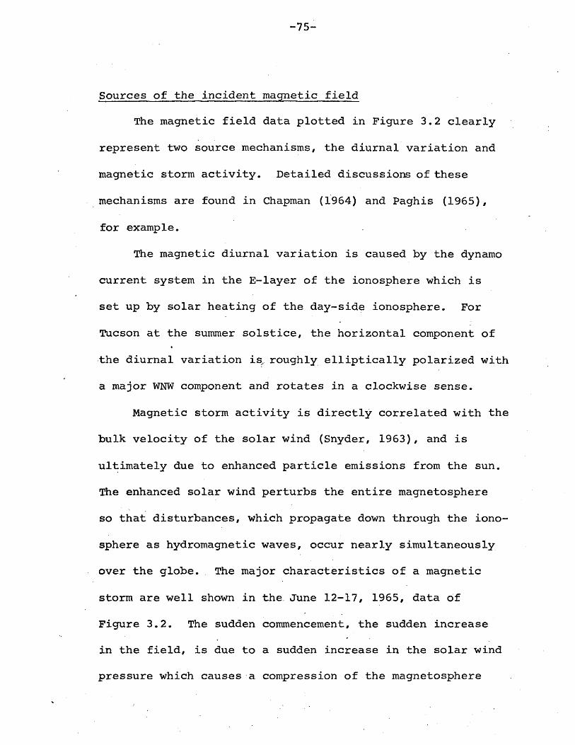
Sources of the incident magnetic field 75
3.2 Electric field measurement 77
3.3 Method of data analysis 82 Higher frequency analysis 83 Lower frequency analysis 87 Sources of error 88
3.4 Magnetotelluric apparent resistivity results 96
Roswell, New Mexico 96 Deming, New Mexico 109 Safford, Arizona 113 Tucson, Arizona 117 Phoenix, Arizona 120 Yuma, Arizona 12~
Gallup, New Mexico 130
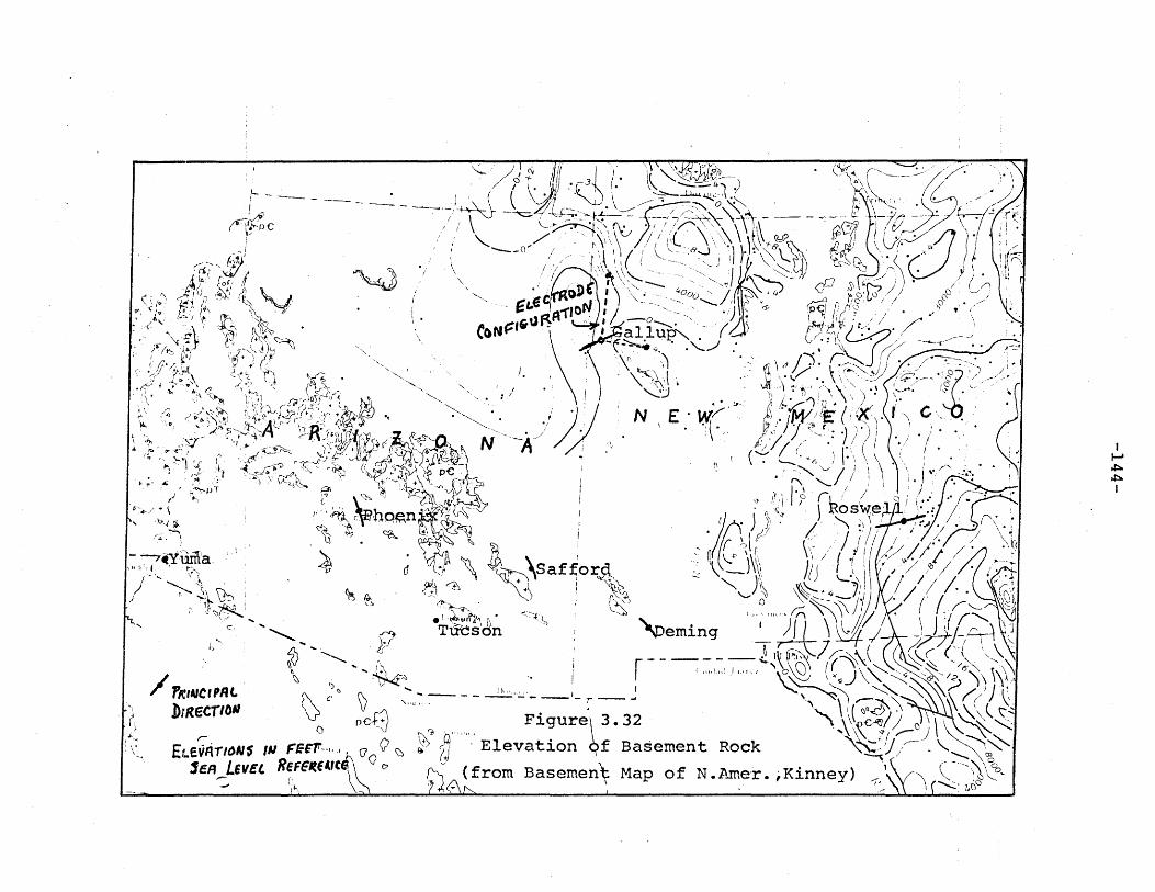
3.5 Interpreted conductivity structure from magnetotelluric apparent resistivities 133
Interpretation of Safford results 134 Interpretation of Roswell and Deming
results 137 Interpretation of Phoenix results 140 Interpretation of Gallup results 142 Disucssion of the Yuma and Tucson results 145 Summary of interpretation 151
CR~PTER 4 - INTERPRETATION OF THE ELECTRICAL CONDUCTIVITY ANOMALY 156
4.1 Electrical conductivity of the upper mantle 156 Upper mantle temperature distribution from
conductivity structure 163
4.2 Correlation of high temperature ?one with other geophysical data 169
Seismic evidence 169 Heat flow evidence 173 Relationship to the East Pacific Rise 175
Page 9
-viii-
TABLE OF CONTENTS (continued)
. --·-----£HAPTER-5---SUGGESTIONS---FOR---FUTURR--WORK --- -- ,----.- ~--'-'--l-a 0
APPENDIX 1 - Error introduced by lumped circuit approximation to a distributed transmission line 182
_APPENDIX 2 - Calculation of the vertical electric field associated with a toroidal B mode diurnal 185
-'-'j:\-PPENDIX 3--.--- -Greenfie1d-algorithm foro-the direct solution of the magnetote11uric network'
. --- ---...equations - --- -------189
APPENDIX 4 - Principal axis and principal values of the magnetotelluric impedance tensor 194
--APPENDIX 5 - Computational details of the sonograrn analysis 198
REFERENCES 201
BIOGRAPHICAL NOTE 211
Page 10
-ix-
LIST OF FIGURES AND TABLES
Figure
2.1 Electromagnetic skin depths .17
2.2 Equivalent network for the spherically stratified conductor 37
2.3 Cantwell-McDonald conductivity model 38
2.4 Electromagnetic fields over a lateral conductivity contrast 41
2.5 Theoretical apparent resistivities over a vertical contact 54
2.6 Theoretical magnetotelluric fields over a vertical contact 55
2.7 Effect of finite-length dipoles on the measured apparent resistivity over a vertical contact 68
3.1 Location map for telluric recording sites 70
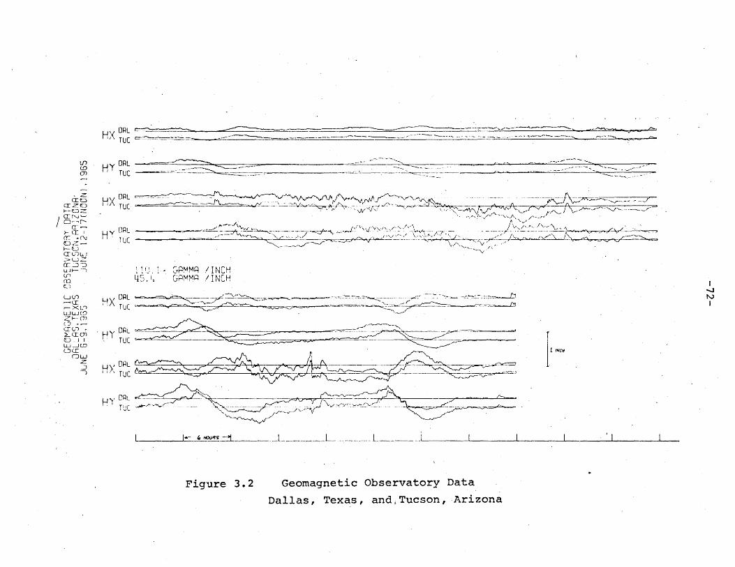
3.2 Geomagnetic observatory data, Dallas and Tucson 72
3.3 Coherency analysis of Dallas and Tucson magnetics 73
3.4 Telluric instrumentation response 79
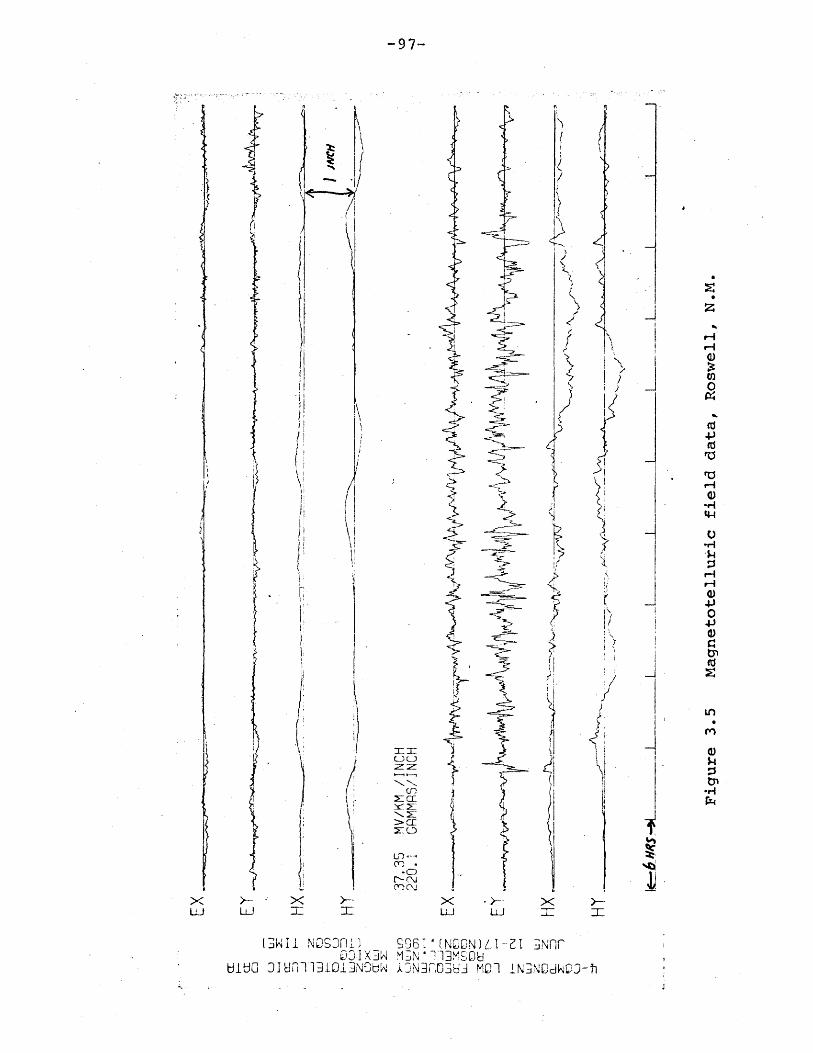
3.5 Magnetotelluric field data, Roswell, New Mexico 97
3.6 Power spectra and coherencies, Roswell, New Mexico 98
3.7 Electric field predictability, Roswell, New Mexico 99
3.8 Time consistency of apparent resistivity estimates, Roswell, New Mexico 101
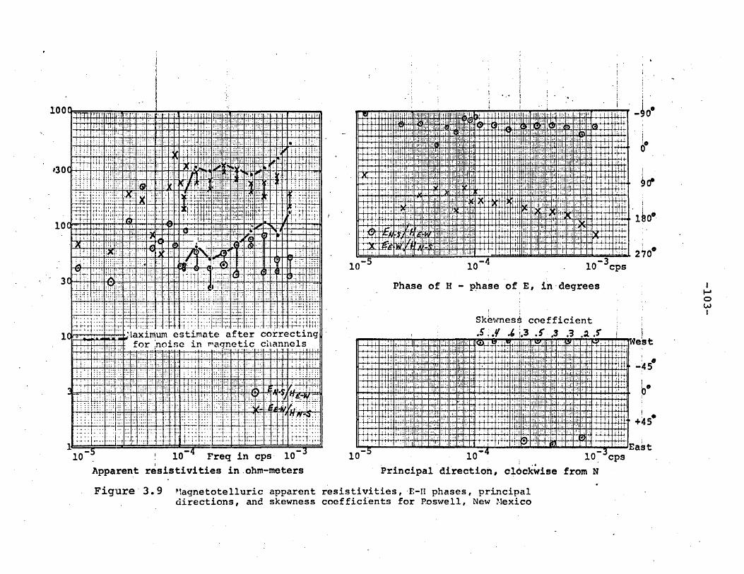
3.9 Magnetotelluric results, Roswell, New Mexico 103
3.10 Electric and magnetic field hodographs, Roswell, New Mexico 107
3.11 Magnetotelluric results using Dallas magnetics, Roswell, New Mexico 108
3.12 Magnetotelluric field data, Deming, New Mexico 110
Page 11
-x-
LIST OF FIGURES AND TABLES (continued)
3.13 Magnetotelluric results, Deming, New Mexico III
3.14 Electric and magnetic field hodographs, Deming, New Mexico 112
3.15 Magnetotelluric field data, Safford, Arizona 114
3.16 Magnetotelluric results, Safford, Arizona 115
3.17 Electric and magnetic field hodographs, Safford and lucson, Arizona 116
3.18 Magnetotel1uric field data, Tucson, Arizona 118
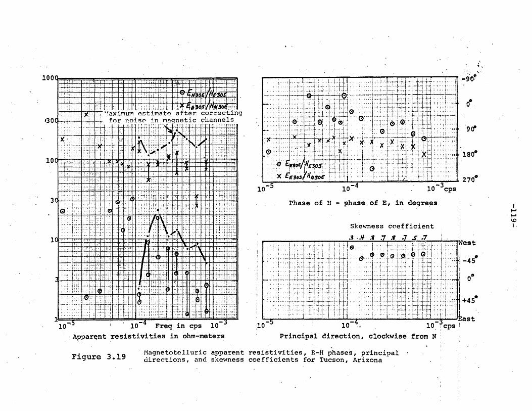
3.19 Magnetotelluric results, Tucson, Arizona 119
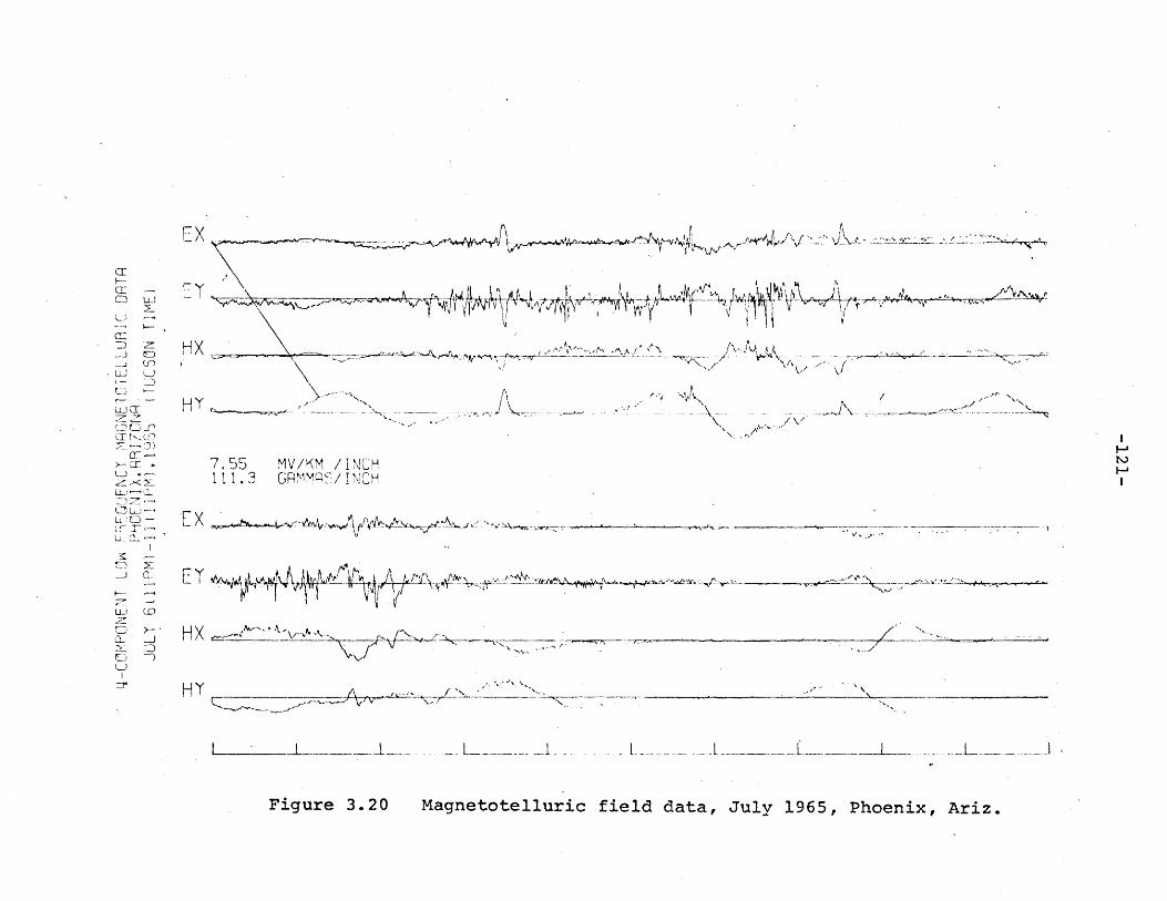
3.20 Magnetotelluric field data, July 1965, Phoenix, Arizona 121
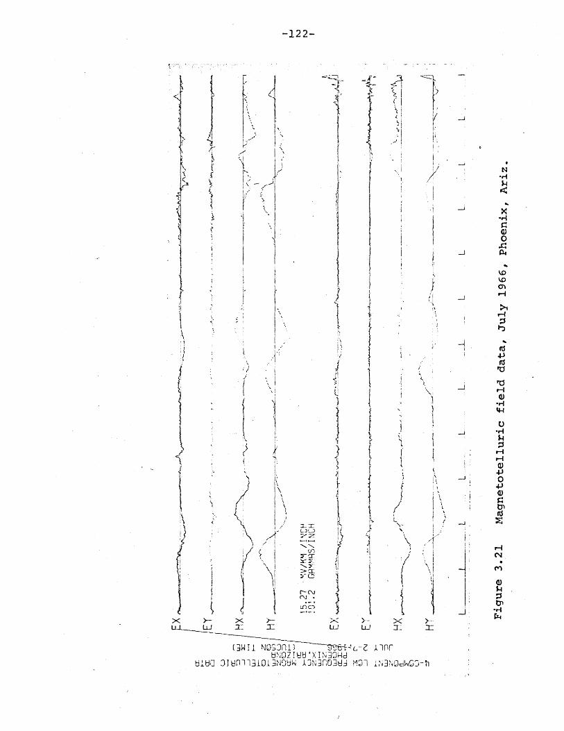
3.21 Magnetotelluric field data, July, 1966, Phoenix, Arizona 122
·3.22 Magnetotelluric results, 1965 data, - Phoenix, Arizona 123
3.23 Magnetotelluric results, 1966 data, Phoenix, Arizona 124
3.24 Electric and magnetic field hodographs, Phoenix, Arizona 125
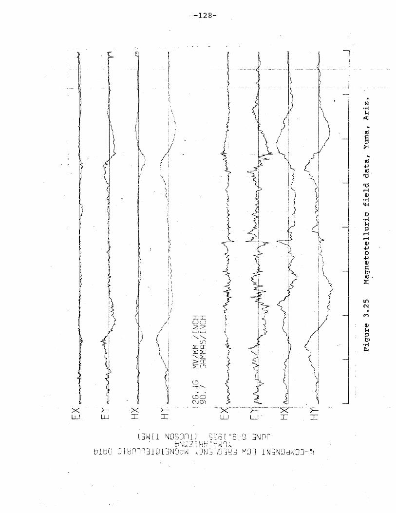
3.25 Magnetotelluric field data, Yuma, Arizona 128
3.26 Magnetotelluric results, Yuma, Arizona 129
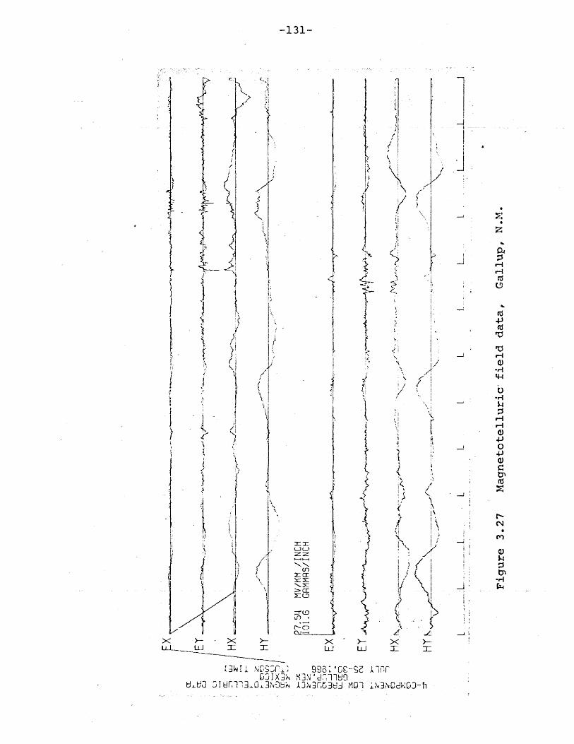
3.27 Magnetotelluric field data, Gallup, New Mexico 131
3.28 Magnetotelluric results, Gallup, New Mexico 132
3.29 Interpreted conductivity structure, Safford 136
-3.30 Interpreted conductivity structure, Deming and Roswel1
3.31 Gravity map of Phoenix area
3.32 Elevation of basement rocks, southwest United States
139
141
144
3.33 Interpreted conductivity structure, Gallup 146
Page 12
-xi-
LIST OF FIGURES AND TABLES (continued)
·---··--·---------------3-.--J4----Sumrnarized- .magnetotellur ic earth conduct i vi ty profiles· 153
3.35 Summarized theoretical apparent resistivity profiles 155
4.1 .. pyrglite stability fields 158
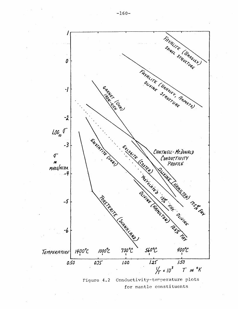
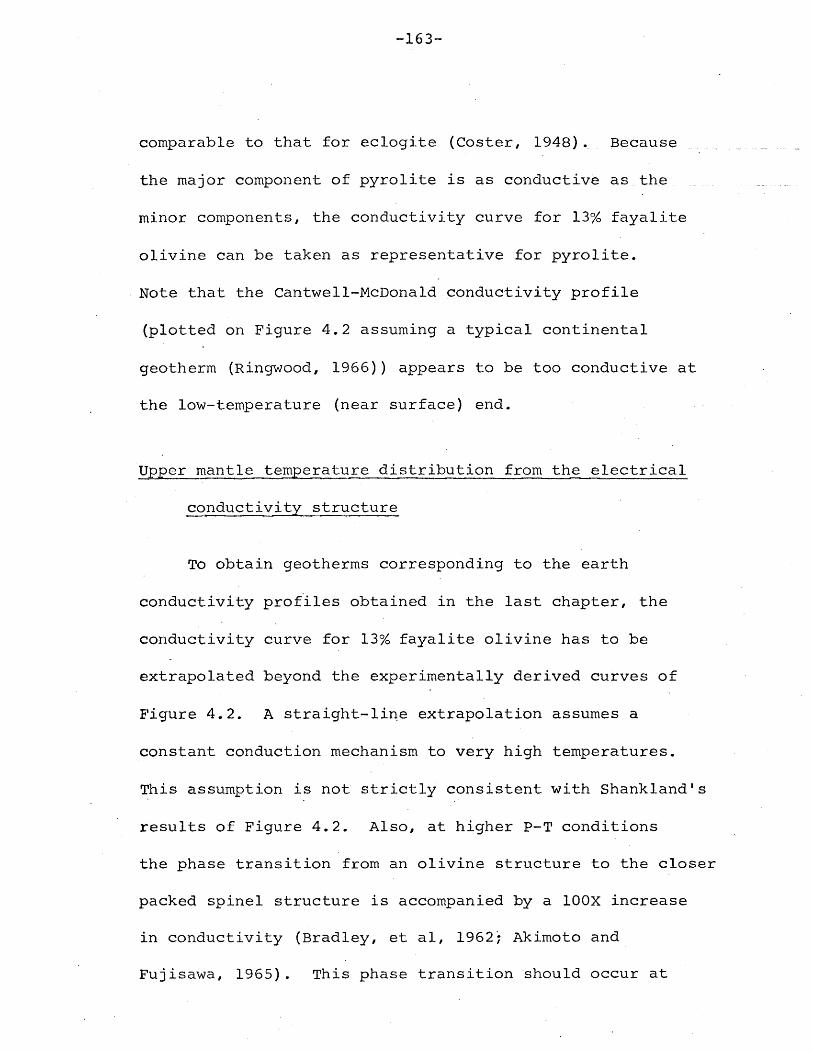
-4.2 Conduct~vity-temperature plots for mantle -.- ----.-.-.- ----'---'-- -_· .. _-.. ··_·-···-·---consti tuents
4.3 pos~ulated temper_ature cross-section
4.4 Seismic evidence for an inhomogeneous upper
160
167
mantle, western united States. 170
4.5 Heat flow measurements, western Unite<;l States 174
4.6 Ceno~oic fault system and extensional tectonic -pattern, western united States 176
A.l Coefficient matrix for network solution 190
A.2 Response of digital filters 199
.. Table"
2.1
3.1
Apparent resistivities for a spherically stratified earth
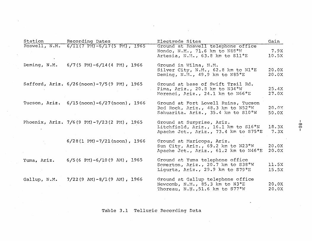
Telluric recording data
3.2 . Representative H t· l/Hh . t 1 ratios, ver ~ca or~zon a Tucson, Arizona
39
80
149
Page 13
-:1-
Chapter 1 - Introduction
1.1 Purpose of investigation
The science of geophysics is the systematic application
of physics to determine the composition and behavior of the
earth and the earth environment. As such, much of solid
earth geophysics consists of the indirect techniques of in
terpreting the internal structure of the earth from surface
measurements. This thesis is concerned with the magneto
telluric method of determining subsurface electrical
conductivity by measuring the electromagnetic impedance of
the earth.
In the upper crust, where conductivity variations can
usually be correlated with differences in rock types and/or
water content, structure has been i~ferred using telluric
current and direct current resistivity methods. In the
mantle, where conductivity variations can usually be cor
related with differences in temperature, conductivity
anomalies have .been detected using geomagnetic induction
. methods.
The magnetotelluric method; which Wi=l~ recogni7.ed in the
early 1950's~ is capable of yielding quantitative infor
mation about the conductivity structure of the crust and
Page 14
-2-
upper mantle. Theoretical and practical difficulties,
however, have plagued the successful application of the
method. The possible non-plane-wave nature of the sources
has been called upon to explain inconsistent data. More
important, the effect of lateral conductivity variations
has not been understood quantitatively. Qualitatively,
the electric currents, prefering to flow in a more con-
ductive medium, may flow in a direction controlled by the
lateral conductivity structure of the local geology rather
than in a direction perpendicular to the magnetic field as
expected when no lateral resistivity contrast is present.
Because the resulting electric field is not always ortho-
gonal to the magnetic field, the measured apparent
_._""
resistivities can be anisotropic.
The original purpose of this thesis was to investigate
the reasons for the anomalously low vertical magnetic field
fluctuations observed at Tucson, Arizona. Small vertical
magnetic fields can be caused by horizontally layered con-
ductive rocks. Tucson is known to be in a zone of
anomalously high electrical conductivity in the south-
weRtern United States (Schmucker, 1964). High apparent
resistivities, however, were obtained by a rough calculation
using diurnal variations of E and H given by Fleming (1939).
Page 15
-3-
Although not definitive in the Tucson region, initial
magnetotelluric data taken by the author in the summer of
1965 in the southwestern united States appeared inter
esting enough to justify further work in 1966 to more
accurately determine the high conductivities and the in
ferred high temperatures associated with the Basin. and
Range province.
In the author's opinion, the contribution of this
thesis is the interpretation of low frequency magneto
telluric data in terms of a petrologically valid upper
mantle conductivity structure in a geologically anomalous
region. Anisotropic apparent resistivity data is inter
preted quantitatively in terms of two-dimensional
conductivity structure, using theoretical values obtained
via a transmission-line analogy due .to T. R. Madden. The
conductivity structure resulting from this magnetotelluric
investigation correlates with other geophysical evidence
to indicate that the anomalous upper mantle in the south
western united States represents an extension of the East
Pacific Rise.
Page 16
-4-
1.2 Brief historical review of the magnetotelluric method
Magnetotelluric theory is the result of a recent
approach towards determining the relationship between tel
luric currents and the geomagnetic field. In 1940 Chapman
and Bartels reviewed the confusing state of the correlation
betvJeen earth-current variations and geomagnetic activity.
Subsequently, by considering the phase relationships
between observed electric and magnetic fields at the surface
of the earth, various workers in the early 1950 l s (Tikhonov
and Lipskaya in Russia: Kato, Kikuchi, and Rikitake in
Japan) discovered the electromagnetic nature of the magneto
telluric field. In 1953 Cagniard published a comprehensive
paper on the theory of the magnetotelluric field within a
horizontally layered earth and on interpretive methods for
obtaining earth resistivity estimates.
Magnetotelluric field data have been successfully
interpreted only for horizontally layered structures:
representative papers are by Cantwell (1960) and Tikhonov
and Berdichevskii (1966). Problems have arisen in inter
preting magnetotelluric'data in areas of lateral conductivity
(Srivastava, Douglctss and WaL'd, 1963, for example).
Further theoretical contributions have considered three
problems - the assumption of a plane incident wave, the
Page 17
-5-
tensor nature of the impedance, and theoretical apparent
-resistivities for two dimensional structures.
Wait (1954) showed how Cagniard's results for a layered
earth are valid only if the fields themselves do not vary
appreciably in a horizontal distance of the order of a skin
depth in the ground. Consequently, the field should be uni-
-form over a considerably-broad area to permit the Cagniard
interpretive procedure to be applied. Price (1962) has
reemphasized this restriction. However, Madden and Nelson
(1964) have considered a realistic earth conductivity pro
file and have concluded that the plane-wave assumption is
valid in most cases.
~or an anisotropic or inhomogeneous earth, the field
apparent resistivity data become anisotropic because the
impedance becomes a tensor quantity. Chetaev (1960),
Kovtun (1961), Rokityanski (1961), Cantwell (1960) and
Bostick and Smith (1~62) have provided schemes to obtain
the principal directions of the conductivity structure.
Wait (1962) has a good review of the Russian work. Madden
and Nelson (1964) have indicated how to calculate the
tensor components using statistical und spectral techniques.
Early discussions of the effect of two-dimensional
conductivity structures centered around the "coast effect".
Page 18
-6-
This effect, an enhancement of the vertical magnetic field
near a coastline associated with an enhanced telluric
field on the land directed towards the coast (Parkinson,
1962~ Rokityanskii, 1963), is due to the lateral contrast
in conductivity between the conductive oceans and oceanic
mantle and the more resistive continents. In the first
quantitative approach, Neves (1957) calculated'apparent
resistivities over dipping interfaces using a finite dif
ference technique, bu·t used the correct boundary conditions
only for the electric field polarized perpendicular to the
strike polarization. d'Erceville and Kunetz (1962)
analytically solved the problem of a fault within a layer
over a half space by expanding the fields in trigonometric
series for the E perpendicular polarization. Weaver (1963)
solved the infinite depth vertical contact problem, again
only correctly for the E perpendicular polarization/by
numerical evaluation of the solution integrals.
Page 19
-7-
1.3 Upper mantle conductivity determinations
As included in an impressive bibliography by Fournier
(1966), presently available'magnetotelluric results are
characterized by the decrease of apparent resistivities
for periods of longer than two hours. This effect is due
to the deeper sampling into the conductive upper mantle
uhder the re~istive crust for increasing period.
Most individual magnetotelluric measurements are
characterized by a limited frequency range and have been
interpreted in terms of a step increase in conductivity.
The depth to this interface and the conductivity beneath
vary widely, with a greater depth required for lower
frequency measurements. These results are indicative of a
continuously increasing conductivity with depth cor
responding to the increasing temperatures.
Earth electrical conductivity information is also
provided by analysis of geomagnetic variations. Chapman
and Whitehead (1923), Chapman and Price (1930), Lahiri and
Price (1939) and Rikitake (1950) have used the ratios of
the internal to external source terms of the earth's
surface potential for the diurnal variations and storm
time transients to essentially define the depth to, and the
conductivity of a conductive mantle. McDonald (1957)
Page 20
-:8-
analyzed the attenuation of the secular variations through
the mantle for conductivity estimates for the lower mantle
and combined his conclusions with those of Lahiri and
Price (1939) for a mantle conductivity profile. Eckhardt,
et al (1963) found that McDonald1s model was adequate to
explain their magnetic fluctuation data of 13.5 day and 6
month periods.
Although these determinations are relatively consistent,
a unique earth conductivity model within narrow limits of
uncertainty is presently unavailable.
Upper mantle perturbations from a radially symmetric
conductivity distribution can be detected using either the
magnetic induction or the magnetotelluric method. For
rough detecti6n, locally anomalous ratios of vertical to
horizontal field components are the magnetic induction
indication of lateral conductivity contrasts. Similarly,
different one-dimensional magnetotelluric proflles at
separated stations are indicative of lateral conductivity
contrasts. For proper interpretation, the magnetic
induction method requires sufficient coverage to separate
the external and the internal fields. Similarly, continuous
magnetotelluric coverage is required for a proper deline
ation of lateral contrasts. Unfortunately, as shown in
Page 21
-9-
the results of this thesis, the magnetotelluric indications
of anomalous upper mantle structures can be lost in the
severe effects of surficial conductivity structure. When
measurements are made parallel to th~ strike of such
surficial structures, however, their effects are greatly
diminished.
The major perturbation from a radially symmetric
conductivity distribution is the conductive ocean and
conductive oceanic mantle. The conductive oceanic mantle,
which is probably due to the increased temperatures
(McDonald, 1963; Clark and Ringwood, 1964), causes the
geomagnetic coast effect. A reverse ocean-effect has been
measured along the coast of Peru (Schmucker, et aI, 1964);
the proximity of an ocean trench could explain the
necessary low temperatures.
The world wide occurrence and geomagnetic interpre-
tations of isolated "upper mantle conductivity anomalies"
has been reviewed recently by Rikitake (1966). These
anomalies are usually pictured as conductive spheres or
cylinders or as variations in the depth to an infinitely
conducting mantle under an
ma·ny anomalies are not satisfactorily explained. The
Japan anomaly, for example, appears to be superimposed upon
Page 22
-10-
a coastline effect. Magnetotelluric measurements are now
being made in some of these anomalous regions to reduce
the ambiguity in the interpretations. However, the Alert
Anomaly in northern Canada has been analyzed by both
techniques without a satisfactory interpretation (Rikitake
"and Whitham, 1964; Whitham and Anderson, 1965; Whitham,
1965). Also, the North German Anomaly, originally attri
buted to a cylindrical conductor at depth (reviewed by
Kertz, 1964), is now interpreted to be complicated by
surface conductivity structures from magnetotelluric data
(Vozoff and Swift). This thesis represents a magneto-
telluric investigation of the conductivity anomaly in the
southwestern united States, originally detected by
Schmucker (1964).
Page 23
, -11-
1~4_ Outline of thesis
Chapter 2, on magnetotelluric theory, first describes
the basic one-dimensional theory and applies it to a
realistic spherically stratified eart~ conductivity
structure to obtain· the effect of finite horizontal wave
lengths in the source field on apparent resistivities.
The equations for an earth with lateral conductivity con
trasts are developed, are transformed into circuit
equations via a transmission-surface analogy, and are
solved numerically via network techniques for theoretical
apparent resistivities. Finally, characteristics of
theoretical and measured impedance tensors are discussed.
Chapter 3 describes the acquisition, analysis, results
and interpretation of magnetotelluric data from the south
western united States. A coherency study of magnetic data
from Tucson, Arizona, and Dallas, Texas, is included to
determine empirically Lhe horizontal wavelengths of the
source field. The technique for obtaining theoretical
apparentresistivities-over -two-dimensional structures is
applied to obtain models necessary to explain the actual
anisotropic apparent resistivity data.
In Chapte,r 4 the resulting electrical conductivity
structure is interpreted geologically_ With reference to
Page 24
12~
laboratory measurements of the conductivity-temperature
relationships of upper mantle constituents, a temperature
cross-section is obtained consistent with the conductivity
structure. Finally, the electrical conductivity anomaly
is correlated with other geophysical data to draw some
, conclusions on the relationship between the North American
continent and the East Pacific Rise.
Chapter 5 includes some suggestions for further work
and is followed by five miscellaneous topics in Appendices.
Page 25
-13-
. ___ . ___ ..... ' ... Chapter. 2 _-. .. ~~gnet,?~elluric Theory
The magnetotelluric method utilizes the boundary con-
ditions forced on the electric and magnetic fields when an
electromagnetic wave propagating thr.ough air interacts with
the earth's surface. Whereas the incident horizontal mag-
netic field is roughly doubled at the surface, the electric
field is strongly dependent upon the earth's conductivity
structure. The essential measurement is the electromagnetic
impedance (the ratio of electric field over magnetic field,
E/H) at the surface.
Since the electric and magnetic fields are vector .
quantities, the impedance is really a 3 by 3 tensor. At
the surface of the earth, where E vanishes, this tensor z
reduces to a 2 by 2 when the horizontal wavelengths are
fixed. For a homogeneous or a layered earth, the.hori-
zontal electric field is only related to the orthogonal
magnetic and the impedance reduces to a complex
scalar. In general, for an: .anisotropic earth (homogeneous
media with Ji= ~j fj ) or an inhomogeneous earth (lateral
··variations of isotropic conductivity) the electric field
is related to both horizontal magnetic field components,
and the impedance must be treated asa 2 by 2 tensor.
Page 26
-14-
Most geophysical disciplines consider progressively
more complicated, and, hence,· more realistic earth models
as theory develops. ·In this chapter, a homogeneous earth
geometry is first considered to develop the basic magneto-
telluric relationships and to calculate the effect of
fi~ite horizontal wavelengths upon the impedance. Then a
plane and spherically stratified earth geometry is con-
sidered using various layered-media techniques. Then a
two-dimensional earth geometry, in which a conductivity
cross section is constant along a strike direction, is
considered to calculate the ·effect of lateral ~onductivity
contrasts. Finally, the properties of the 2 by 2 impedance
tensor are discussed.
2.1 Relationships from Maxwell's Equations
In the following derivations in Cartesian co-ordinates,.
the geomagnetic ~o-ordinate convention will be used, with
x - north: y - east: and z - down. In homogeneous isotropic
media, in the absence of sources, Maxwell's equations in the
rationalized MKS system are
rj>fE 'Ji5
-::: &t 2.1-1
J of-e>D
f/xH --. 2.1-2 -- at
t!.j) . ~ j? - 0 - ·2.1-3
Page 27
15-
\l- 13 :::: 0 2.1-4
where J-: (j E )
... £wt .By assuming e time dependence, these equations reduce
to
9'x £ -- 2.1-5
rJxl/ u£ - ifi/€ E 2.1-6
It is standard procedure to combine-these two equa-
tions into the vector Helmholtz equation
2.1-7
This formulation emphasizes the wave nature of the solutions
In electromagnetic propagation in the earth at magneto-A -
telluric freque~cies (W < lO~ cps), the propagation
constant is dominated by the conduction current term (ilJ/)'rr),
and the Helmholtz equation becomes a diffusion equation.
Page 28
-16-
The -solution field does not freely propagate, but
exponentially decays with depth; this decay, dependent upon
the conductivity and frequency, is called the "skin effect".
The skin depth, defined as that depth at which the fields
reduce to lie of the surface value, affords a rather crude
qualitative estimate of an effective "depth of penetration".
Skin depths, ~ '" -I};~ "1, are given in Figure 2.1 as a
function of Q and W , assuming a free space value for/,-" •
Therefore, the frequency range appropriate for a magneto-
telluric investigation depends upon the depths of interest.
The conduction current term is much greater than the
displacement current term for most magnetotelluric instances
and the propagation constant in the ground is much greater
than in the air:
Thus, the earth has a high refractive index with respect to
the air, and incident waves will be refracted almost
straight down, regardless of the angle of incidence.
The impedance relationships are dependent on the spatial
variations of the incident field, not on the nature of the
source itself. The source of the electromagnetic energy
depends upon the frequency range involved; the sources for
the low frequency magnetotelluric data analyzed in this thesis
Page 29
-17-
~------~------~------~------~-------mQ
/02.. ~
I~ /0
/.0
0.1
/0-5 /0-'1 /0-3 /O-:t
f diUrr!al 2
t hour 15 min. Frequency
period period period in
Figure 2.1 Electromagnetic Skin Depths as a Function of Frer:Il1pncy rlnri Resistivity.
cps
~ I ?~ ~ ...... 0
r: • ..-l
~ +l • ..-l :>
• ..-l +J tf1
• ..-l U)
CJ ~
Page 30
18':'
are discussed in Chapter Ill.
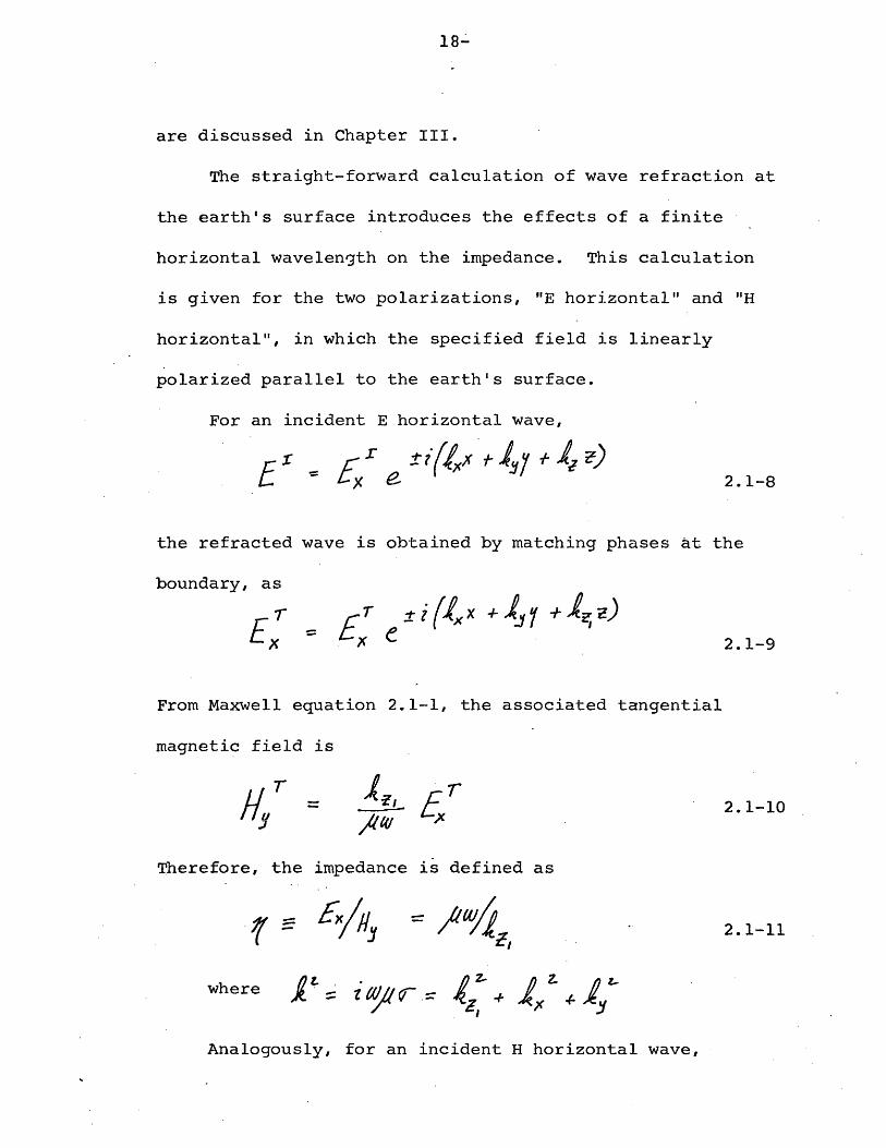
The straight-forward calculation of wave refraction at
the earth's surface introduces the effects of a finite
horizontal wavelen~th on the impedance. This calculation
is given for the two polarizations, liE horiiontal ll and "H
horizontal ll, in which the specified field is linearly
polarized parallel to the earth's surface.
For an incident E horizontal wave,
2.1-8
the refracted wave is obtained by matching phases at the
boundary, as
Er x 2.1-9
From Maxwell equation 2.1-1, the associated tangential
magnetic field is
2.1-10
Therefore, the impedance is defined as
2.1-11
where
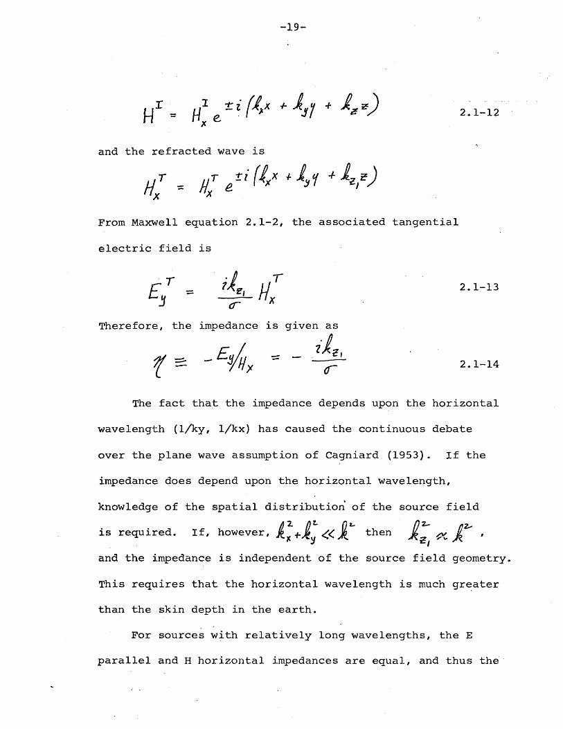
Analogously, for an incident H horizontal wave,
Page 31
-19-
2.1-12
and the refracted wave is
From Maxwell equation 2.1-2, the associated tangential
electric field is
-r i)e, T Ej - Hx er
2.1-13
Therefore, the impedance is given as
1(=== _£~)l - it.z, -0- 2.1-14
The fact tha~ the impedance depends upon the horizontal
wavelength (l/ky, l/kx) has caused the continuous debate
over the plane wave assumption of Cagniard (1953). If the
impedance does depend upon the horizontal wavelength,
knowledge of the spatial distribution' of the source field
is required. If. however. A.;.,.i; «1<- then i;' ~Jz.- . and the impedance is independent of the source field geometry.
This requires that the horizontal wavelength is much gr~ater
than the skin depth in the earth.
For sources with relatively long wavelengths, the E
parallel and H horizontal impedances are equal, and thus the-
Page 32
-20":'
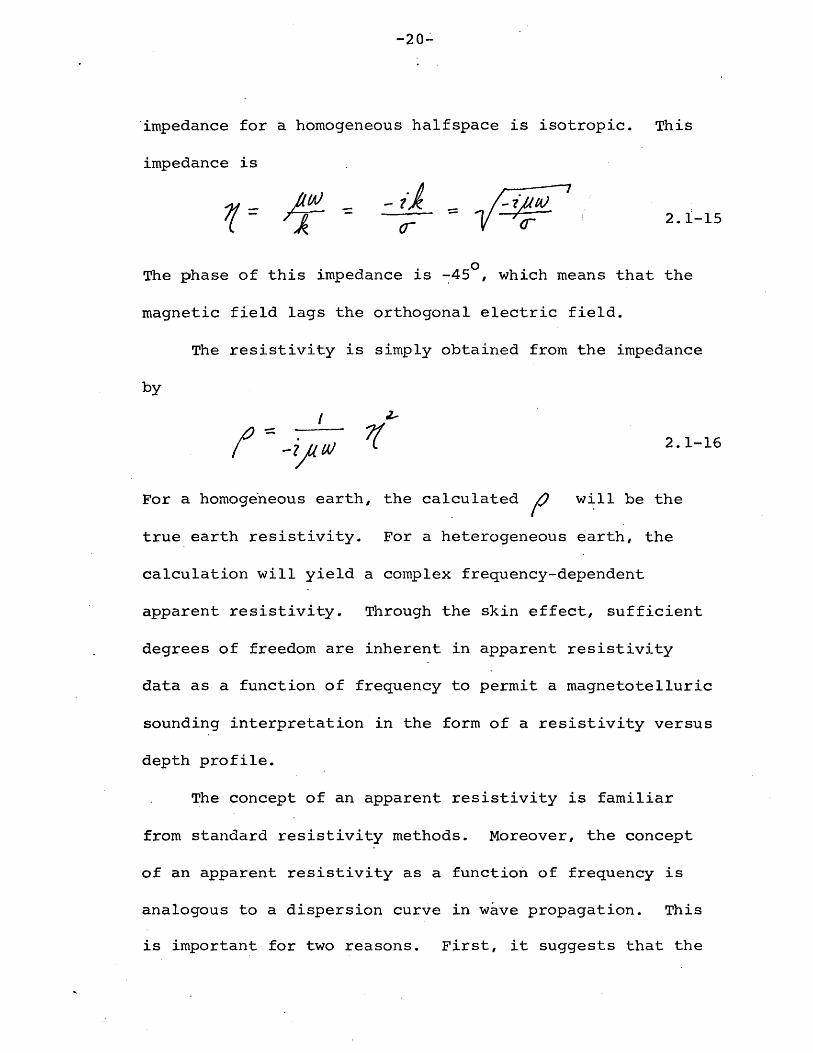
"impedance for a homogeneous halfspace is isotropic. This
impedance is
1(= 2.1-15
The phase of this impedance is ~45°, which means that the
magnetic field lags the orthogonal electric field.
The resistivity is simply obtained from the impedance
by
I
2.1-16
For a homoge"neous earth, the cal~ulated f will be the
true earth resistivity. For a heterogeneous earth, the
calculation will yield a complex frequency-dependent
apparent resistivity. Through the skin effect, sufficient
degrees of freedom are inherent in apparent resistivity
data as a function of frequency to permit a magnetotelluric
sounding interpretation in the form of a resistivity versus
depth profile.
The concept of an apparent resistivity is familiar
from standard resistivity methods. Moreover, the concept
of an apparent resistivity as a function of frequency is
analogous to a dispersion curve in wave propagation. This
is important for two reasons. First, it suggests that the
Page 33
-21-
·the impedance is as physically important as, say, the phase
velocity. Secondly, it indicates that the determination
of the conductivity distribution from apparent resistivity
data is a typical geophysical inverse boundary-value
problem.
Page 34
-22-
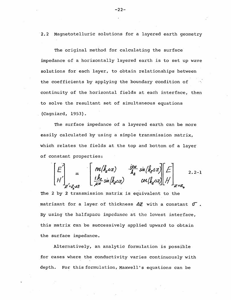
'2.2 Magnetotelluric solutions for a layered earth geometry
The original method for calculating the surface
impedance of a horizontally layered earth is to set up wave
solutions for each layer, to obtain relationships between
the coefficients by applying the boundary condition of
continuity of the horizontal fields at each interface, then
to solve the resultant set of simultaneous equations
(Cagniard, 1953).
The surface impedance of a layered earth can be more
easily calculated by using a simple transmission matrix,
which relates the fields at the top and bottom of a layer
of constant properties:
[ :1, ;! -=~-AC
2.2-1
The 2 by 2 transmission matrix is equivalent to the
matrizant for a layer of thickness LlZ with a constant a. By using the halfspace impedance at the
this matrix can be successively applied upward to obtain
the surface impedance.
Alternatively, an analytic formulation is possible
for cases where, the conductivity varies continuously with
depth. For this formulation, Maxwell' s equations can be
Page 35
-23-
rearranged into a form also convenient for matrix method
solutions. For the H horizontal polarization, where
H = H = E = 0, and ~x [ ] == DJ y Z x
J./ ;v e !:i (~y + Jl i) X
Maxwell's equations
d J./X
02-
'0 !Ix '0'1
~E2
OV
By removing E , z
are
- fTEj
== - aEZ
-oEy fl'alfIx -.o~
-1Lu; 1/)(+ ~ (- ~ ~~~)
_ -lbw (I / _ j.}- \ 1/ :/- X-;:) I7x
2.2-2
2.2-3
2.2-4
2.2-5
2.2-6
Equations 2.2-2·and 2.2-6 can be combined into a matrix
formulation,
2.2-7
Page 36
-24-
Analogously, the E horizontal polarization case can be
represented as:
2.2-8
For an expression directly in terms of the impedance,
I ()~ --H oc E ~H --Ht. oZ 2.2-9
Thus, for the H horizontal polarization,
) (t) -::: - (-~w(/ - f,J4) - {J (uEj) 2.2-10 O~ Hx
or
d Z - - (j Z:l. -)"W (1- f) - 2.2-11 oi! -
And, unulogously, for the E horizontal polarization,
2.2-12
Equations 2.2-11 and 2.2-12 are Riccati equations for the
impedance.
Page 37
-25-
Another method interprets the surface impedance of a
layered earth as being analogous to the impedance of a non-
uniform transmission line. This approach has been used
previously by Madden (1966; Madden and Nelson, 1964; Madden
and Thompson, 1965) and its influence permeates this entire
thesis.
This transmission line analogy is motivated by the
similarity between Maxwell's equations governing the ortho-
gonal components of E and H and the transmission line
equations governing current and voltage on a transmission
line. This analogy emphasizes the role of the impedance as
the important physical parameter relating E and H, and
suggests that the cross-coupled first order partial differ-
ential equations are in a sense more basic than the derived
uncoupled wave equation. The transmission line equations
are
JV --? I
Zj -z: 1 2.2-13
JI -YV 2.2-14 -- -tit
or
j [ j] [ 0 -~ [:] 2.2-15 -dt -y
Page 38
-26-
where Z is the series impedance per unit length and Y the
shunt admittance per .unit length. Combining equations
2.2-13 and 2.2-14 yields wave equations for V and I, with
a propagation constant k giveri by
2.2-16
The characteristic impedance is defined by
z 2.2-17
The basic analogy is between equations 2.2-15 and
either 2.2-7 and 2.2-8. By associating E with V and H
with I, or vice versa, the distributed circuit parameters
of the equivalent transmission line are given in terms of
the earth parameters involved. A lumped circuit approxi-
matibn results which can be solved using standard network
techniques. Note that the propagation constant and
characteristic impedance are given by
2.2-18
2.2-19
Page 39
-27-
Although the transmission matrix of equation 2.2-1 was
used to generate theoretical magnetotelluric apparent
resistivity type-curves for multi-layered cases, the
transmission-line analogy was developed and extended to a
transmission-surface analogy for two-dimensional earth
geometries. The maximum layer thickness restriction and
the effect of thick layers on the surface impedance is
discussed in Appendix 1.
Various authors (Cagniard, 1953; Yungel, 1961; and
Wait, 1962) have presented two and three layer magneto
telluric type curves and discussed typical resolution
problems such as that of a thin resistive layer.
Page 40
-28-
2.3 Impedance of a spherically stratified conductor
Since the assumption of infinite horizontal wavelengths
becomes less valid at low frequencies, while simultaneously
the increased skin depth becomes a significant fraction of
the earth's radius,it is desirable to calculate the
impedance of a spherically stratified conductor for any
given horizontal wavelength. Wait (1962) and Srivastava
(1966) have approached this problem via the standard method
of setting up wave soluti9ns in spherical shell~, . then
solving the resultant problem in terms of spherical Bessel
functions. Complications in the evaluation of the Bessel
functions limit the usefulness of this approach. However,
the calculation of the impedance of a spherically stratified
conductor is a good example of the transmission line analogy
approach.
Solutions to the vector wave equation in spherical
coordinates for a homogeneous region can be represented by
a complete set of orthogonal vector solutions, designated as
L, M, and N by Stratton (1941). The Hand E fieids can be
completely represented by the M and N solutions:
H = j ?? (~KJf !1~~ r b~u #;nJ E --1 ff (pPf~~~ r ~t#~~)
2.3-1
2.3-2
Page 41
-29-
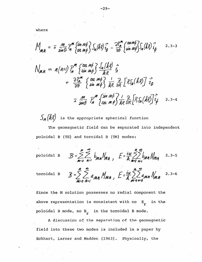
where
2.3-3
2.3-4
SA (A.~ is the appropriate spherical function
The geomagnetic field can be separated into independent
poloidal B (TE) and toroidal B (TM) modes:
poloidal B
toroidal B
since the M solution possesses no radial component the
above representation is consistent with no E r
poloidal B mode, no B in the toroidal B mode. r
in the
A discussion of the separation of the geomagnetic
field into these two modes is included in a paper by
Eckhart, Larner and Madden (1963). Physically, the
2.3-5
Page 42
-30-
horizontal ionospheric electric currents, which are the
primary generating sources for low-frequency geomagnetic
energy, produce a predominantly poloidal B field. More-
over, the vertical electric field in the air that would be
associated with a toroidal B mode diurnal variation is
unrealistically large (Appendix 2).
Theoretically, the impedance for any harmonic of each
mode is isotropic, a result implied by the spherical
symmetry.
MAl( El} . lcK J;(1R) =: -!i ~JJB T- 2.3-7 - - - . lR. [ 1?5".(Jd?)j liD H1'
Z"~ Cf)- . Crz [RSA((iRJ] '" _4 -::. - - !..UfY- 2.3-8 -- - ~R~ (AR) -iiut/JB Hq, l Hff
However, even in a homogeneous medium, the impedance is not
constant with depth since the geometry is constantly
changing.
To use the transmission line analogy approach, a matrix
formulation of Maxwell's equations for each harmonic of the
poloidal B mode must be developed. In spherical co-ordinates, • ..L -zw I
and with e time dependence, Maxwell 1 s equations expand
into:
Page 43
-31-
2.3-9
-1- [-lA (1/ Ef ) ] - -iaIjA I/r; 2.3-10
I [ J; (AE~) ] - i W)< Ill-- -11
2.3-11
and
J [- ~ (Ill/if» ~ ,
()!l1I ] crEr;-- 2.3-12 -- siM(). Ft = It
J [ ~ (/I 110) ~~-J <rEp 2.3-13 - - -A.
[ l& (;v" (J 114) ()If~] - 0 2.3-14 Otp
where EA., is zero in the po1oidal B. mode. Equation 2.3-14
is consistent with the solutions of equations 2.3-3 through
2.3-5. Similarly from these solutions,
I ra JlII [~ M(;ltfV J (, £) - - hILL It &. siAt~ o? 2.3-15
?HIl [-~ A(Affi ] (/lEy :::. ~Il"/' ~ '()~
2.3-16
Page 44
-32-
With equation 2.3-15, -equation 2.3-12 reduces to
2.3-17 .
with equation 2.3-16, equation 2.3-13 reduces to
f; (11 lis) - ( Q - ~(t11ffL) ( It [ ) 2.3-18
1)J Wit!. 4-
Combining equations 2.3-10, 2.3-11, 2.3-17, and 2.3-18
to re~ove HA) Maxwe11's equations can be expressed as
ll.f; 0 -~W 0 0 11 E(;
d Il. H ~ q-_ ~(~1I·t) 0 0 0 f) 1/ 9- 2.3-19 - - ~/.I.IAL
BA AE~ 0 0 0 -tjAW /lE~
A Hr 0 0 ,tt(M+I) _ r ~lIJlat
0 Il /{~
This 4x4-matrix uncouples into two independent po1arizations
with coefficient matrices differing only in sign. The dif--
.. All Es. £<J; ference in sign is due to Z :::: - -= - - ,thus
Htf Htr the impedance is isotropic, as indicated in equation 2.3-7.
The 2x2 relationships
2.3-20
Page 45
-33-
differ from the flat earth case in that !lE and ItH are the
cross-coupled variables, rather than E and H, but the im-
pedance is maintained as E H
A Riccati equation for the impedance is easily derived
from the equations 2.3-10 as
2.3-21
A quirk in spherical geometry makes this equation, and
equation 2.3-7 for the impedance, independent of m. Since
m must be less than n, a large m requires a large n.
For reference, equation 2.2-15 for the flat-earth imped-
ance case can be expressed as
2.3-22
The flat-earth long horizontal wavelength approximation,
transforms in the spherical earth case to
2.3-23
This ineqality will not hold for values of ~ near the
center of the earth. Due to the skin effect, however, only
Page 46
-34-
very low frequency variations will penetrate deep enough
in an earth with conductivity increasing with depth to be
perturbed by the sphericity.
Transmission-line analogy formulation and solution
A transmission-line analogy calculation for the surface
impedance follows directly from equation 2.3-20.
To make valid transmission-line associations, energy
must be conserved. This restriction essentially normalizes
the equivalent transmission line variables with length
parameters and results in a non-uniform transmission line.
For a spherical geometry.
2.3-24
Since A E and A 1-/ are the variables in equations
2.3-20 and since an impedance of E/H is desired, the
appropriate associations are
2.3-25
2.3-26
Page 47
-35-
with these associations, the distributed impedance and
admittance expressions consistent with 2.3-20 and the
transmission line equations are
L=
y --
Note that
'i ~ OIlL -1f4(AfIl) Z)tt<l/lL
I
2.3-27
2.3-28
2.3-29
2.3-30
For calculation an equivalent network is constructed by
sectioning a conductivity model into layers of thickness
much smaller than a skin depth. Since the lumped impedance
and the lumped admittance are proportional to the distance
between nodes, the lumped parameters are
-z"? Ll 2.3-31
_ (.1"WjJ ~/l.1.. - .M {fitf /21 D 1)1. w /tl. /
2.3-32
Page 48
-36-
where ~ is the layer thickness. For thin layers far from
the center of the sphere, the radius to the middle of the
layer can. be used for n. The terminal impedance is the
characteristic impedance of the homogeneous inner sphere.
This equivalent network is diagramed in Figure 2.2.
Using the Cantwell-McDonald earth conductivity profile
(McDonald, 1957; Cantwell, 1960), which is plotted on
Figure 2.3, a 320 layer model was solved for the surface
impedance. Apparent resistivities and phases are given in
Table 2.1 for a range of spherical harmonic orders and fre
quencies. For the non-physical zero order, the results are·
equivalent to the infinite horizontal wavelength flat-earth
geometry and are given for comparison to show the effect of
sphericity. The minimum wavelength, at which the estimated
apparent resistivity differs by an arbitrary twenty per cent
deviation criterion, is indicated in Table 2.1.
Page 49
-37-
----------_._--------....---
-----------------
11.J,.
r:J _-] J!..N:!..
----r-~-----~5------------
where:
Figure 2.2
Q - N layers ~., J'-' 0;, ~:- Ufl
( Z·(j)1J.. 6i ft.i :t _. lit (/}[f I)) -I i uftnf t1J-i
~ (- iWjA) 6./j-z·
~ ~/~~j ~
Equivalent network for the
spherically stratified conductor.
Page 50
-38-
DEPTH CONDUCTIVITY
10S" (km) (mhos/meter) -4
Lower 0 1.0x10
ID'" Core 20 -4
1-1antle 1.0xlO -4 40 1.0xlO.
103 ~ . -4 Cl) 60 1.0xlO +J (J)
80 -1 ~ .20x10 "- -I
ID'" 00 100 .22xlO 0
-1 ~ 125 ~ .25xlO
~ 150 -1 10 .28xlO
• .-1 -1
~ 200 .32xlO .p . -1
I • .-1 -300 .42x10 :> . -1 • .-1
400 +> .50x10
10-1 0 ~ 600 .10 re ~ '700 .50 0
10-;1. CJ 1 800 .30x10
Upper 2 900 .10xlO Crust r1antle . 2 10-3 1000 .20xlO
2 1500 .30xlO
/011
2000 . 2
.60x10 .
30 /I 300 11;00 . '3000 2500 3 .12x10
2850 .' 3
Depth in kms .20x10 5 2898 I.OxlO
Figure 2. 3 Cant\'!ell-~IcDonald conductivity model
Page 51
-39-
MAGNETOTEllURIC APP'~ENT RESISTIVITIES FOR SPHERIC.(LY STRATIFIED EART~ FC~ VARIOUS SPHERICAL MODE ORDERS
CAN1WELL-HCCONAlC CO~[UCTIYITY MODEL
FREQ RESISTIHTIES IN Of-"-P4ETERS
1t4 CPS ~. 0 2 It 9 1& 36 lOO
I I.OOE-07 .12E :n .1 lE 01 .10E 01 I .76E 00 .]lE 00 .89E-Ol .23E-Ol .32E-02
• litE-Ob .14E 01 .UE 01 .13E ~l I .95E 00 .ItCE 00 .12E 00 .12E-01 .ItU-02 .19E-06 .22E 01 .2 "E 01 .18E 01 I • lItE 01 .5r;E 00 .l1E 00 .1t6E-lll .6lE-02 .27E-Ob .24E 01 .2~E 01 .22E 01 I .HE 01 ".77E 00 .23E 00 .63E-il1 .84E-02 • HE-Ob .HE ~l .BE 01 .HE 01 I .2ltE Cl .1lE 01 • HE 00 .88E-Ol .12E-Ol .52E-Ob .,.2E !U .ItCE 01 .39E 01 I .31E 01 .IItE 01 ."5E 00 .12E \)0 .16E-Ol .72E-Ob .~5E 1)1 .53E 01 .50E 01 I .41E 01 .2lE 01 .61tE 00 .17E 00 .23E-01
1.OOE-Ob .7lE 01 .6EE 01 .64E ~1 I .53E 01 .21E 01 .88E CO .BE 00 .32E-Ol • lite-OS .I!7E 1)1 .8 I!E 01 .B2E ')l I .69E 01 .31E Jl- .12E 01 .33E 00 .ItItE-Ol .19E-OS .l2E 02 .lIE 02 .1IE 02 L.92E 01 .50E 01 .l7E 01 .1t6E 00 .6lE-01 .27E-05 .14E n .1ltE ~2 .BE 02 :Ue-o"2l .6t:E 01 .23E 01 .63E 00 .84E-Ol .HE-O'; .17E 02 .16E 02 .16E 'J2 .lItE 02 I .8tE 01 .32E 01 .86E 00 .12E 00 .52E-05 .2lE n .2 E 02 .19E 'J2 .18E 02 I .12E 02 .1t4E 01 .12E 01 .16E 00 .12E-05 .25E J2 .25E 02 .HE 02 .22E 02 I .15E 02 .61E 01 .l7E 01 .23E 00
I.OOE-OS .2SE 02 .2 I!E 02 .27E 02 .25E 02 I .1 fE 02 .82E 01 .23E ;)1 .31E" 00 , .IItE-04 .34E 02 .3~E 02 .HE n .32E 02 I .2~E 02 .llE 02 .33E 01 .44E 00 .19E-04 .38E 02 .38E 02 .38E 02 ". 36E 02 L .:.Ut.9l. .15E 02 .45E 01 .6lE 00 .27E-04 .,.2E 02 ."~E 02 ."lE 02 .40E 02 • 3~E 02 1 .20E 02 .63E 01 .85E 00 • 37E-04 .lt4E 02 .4~E 02 .HE 02 .1t3E 02 .leE 02 I .25E 02 .S5E 01 .12E 01 .52E-04 .,.9E 02 .It 9E 02 .~9E 02 ."8E 02 .1t~E 02 I .HE 02 .12E 02 .16E 01
", • lZE-04 .53E 02 .5~E 02 .53E 02 .52E 02 .4~E 02 I .l8E 02 .16E 02 .23E 01. I 1.00E-04 .59E n .5«;E 02 .59E 02 .58E 02 .55E 02 1 .45E 02 .21E 02 .llE 01 .14E-Ol .t 5E 02 .6~E 02 .64E 02 .64E 02 .62E 02 -.53EOz1 .2SE 02 .44E 01 .19E-03 .73E 02 .12E 02 .72E 02 .72E 02 .7eE 02 .61E 02 I .37E 02 .6lE 01 .27E-03 .e2E n .81E 02 .81E 02 .BlE 02 .79E 02 .71E 02 J .1t7E 02 .84E 01 .HE-Ol .BE 02 .93E 02 .92E 02 .92E 02 .8CjE 02 .82E 02 I .58E 02 .12E 02 .52E-03 .11E 03 .HE 03 .11E 03 .11E 03 .1CE 03 .96E 02 I .72E 02 .16E 02 .12E-03 .12E 03 .UE 03 .12E 03 .12E 03 .12E 03 .1lE 03 I .8SE 02 .22E 112
1.00E-03 .1ltE '3 .14E 03 .lltE I) 3 .1ltE 03 .lItE 03 .13E 03 I, .1lE 03 .31E 02 .HE-02 .l7E 03 .liE 03 .17E 03 .l7E 03 .17E 03 .16E 03 L.13E D3 .42E 02 .19E-02 .HE 03 .2JE 03 .21E 03 .21E 03 .2CE 03 .19E C3 :-lTE-oT1 .51E 02 .27E-02 .25E 03 .2~E 03 .25E 03 .25E 03 .25E03 .24E 03 .20E 03 I .18E 02 .HE-02 .HE 03 .31E 03 .31E 03 .3lE 03 .31E 03 .30E 03 .26E 03 I .10E 03 " .52E-02 .l8E 03 .HE 03 .3eE 03 .38E 03 .)sE 03 .37E 03 .32E 03 I .14E 03 .72E-02 .48E 03 .4~E 03 .HE 03 .UE 03 .4eE 03 .46E 03 .4IE 03 I .19E 03
1.00E-Ol .HE 03 .61E 03 .61E 03 .61E 03 .61E 03 .59E 03 ".53E J3 I .25E 03 I
FREQ IMPEDAN CE PHASE IN "EGREES
IN CPS 1\- 0 1 2 4 9 18 36 100
1.00E-07 -le.9 -19.5 -80.5 -83.4 -&8.3 -89.9 -90.0 "-90.0" • 14E-06 -n.7 -80.2 -8C.9 -83.5 -88.2 -89.9 -90.0 -90.0 .19E-Ob -78.7 -79.5 -80.4 " -82.9 -87.9 " -89.8 -90.0 -90.0 .21E-06 -7«;.4 -79 .7 -80.7 "-83.0 -87.6 -89.7 -90.0 -90.0 • 37E-06 -78.S -19.2 -79.9 -82.2 -87.3 -89.7 -90.0 -90.Q .52E-Ob " -78.6 -19.0 " -79.6 -81.9 -86.9 -89.6 -90.0 -90.0 .12E-06 -71.8 -78.2 -79.0 -81.1 -86.3 -89.4 -89.9 -90.0
1.00E-06 -76.9 -77 .3 -78.1 -80.3 -85.7 -89.2 -89.9 -90.0 .lItE-05 -76.0 -76.2 -71.0 -79.2 -84.9 -89.0 -89.9 -90.0 .l9E-OS -1".4 -1".8 -75.6 -77.7 -83.9 -eS.7 -89.8 -90.0 .21E-05 -73.1 -73 .3 -71t.1t -16.3 -82.7 -88.2 -89.8 -90.0
".HE-OS -H.6 -72 .0 -72.6 -7".7 -81.3 -87.1 -89.7 -90.0 .52E-05 -6«;.b -70.0 -70.8 -72.7 -19.5 -87.0 -89.6 -90.0 .12E-05 -67.5 -67.6 -68.5 -70." "-11.4 -86.0 -89." -90.'
I.GOE-OS -66.2 -66.4 -66.9 -68.7 -15.5 -84.8 -89.2 -90.0 " .1ItE-04 -63.1 -63.8 -6".1 -65.9 -12.8 -83.2 -88.9 -90.0
.19£-04 -61.1 -61.8 -62.3 -64.0 -70.3 -81.3 -88.4 -90.0
.27E-04 -6C.6 -60.7 -61.1 -62.5 -68.0 -19.2 -81.9 -89.9
.HE-Olt -60.2 -60.2 -60.8 -61.7 -66.5 -17.0 -81.1 -89.9
.52E-0" -5t;.5 -59.5 -59.9 -60.7 -64.6 -14.5 -86.1 -89.9
.12E-04 "-59.8 -6Q.0 -60.1 -60.8 -63.8 -72.4 -14.8 -89.8 I.ClOE-04 -6IJ.i -60.2 -60.3 -60.9 -63.5 -70.6 -83.3 -89.8
• litE-DJ -61.0 -61.0 -61.2 -61.5 -63.4 -69.4 -81.6 -89.7 .l9E-O] " -61.1 -61.8 -61.8 -62.2 -63.7 -68.5 -79.9 -89.6 .21E-OJ -62.1 -62.S -62.9 -63.1 -64.3 -68.1 -78.2 -89.4 .nE-O} -63.9 -63.9 -64.0 -64.2 -65.2 -68.3 -11.0 -89.2 .52E-0} -65.3 -65.3 -65.3 -65.4 -66.1 -68.6 -16.0 -S8.Cl .72E-O} -66.5 -66.5 -66.5 -66.7 -67.3 -69.3 -75.4 -88.5
I.COE-O] -68.0 -68.0 -68.0 -68.1 --68.5 -70.1 -15.2 -88.1 .11tE-02 -6~.3 -69.1t -69." -69.5 -69.8 -11.1 -75.3 -87.6 • 19E-02 -7e.8 -10."S --70.S -70.9 -71.1 -72.2 -15,6 -87.1 .27E-02 -72.2 -72.3 " -12.3 -72.3 -12.5 -71.3 -76.2 -86.6 • 37E-Ol -73.5 -71.5 -73.5 -73.5 -73.7 -74.4 -76.8 -86.2 .52E-02 -7,..S -74.8 -7".8 -74.9 -75.1 -15.6 -17.6 -85.9 .12E-02 -76.0 -76.l -76.0 -76.0 -16.2 -16.6 -78.3 -85.7
l.COE-02 "-77 .1 -11.1 -71.1 -17.1 -77.2 -77.6 -79.0 -85.6
Table 2.1
Page 52
-40-
2.4 Magnetotelluric relationships for a two-dimensional
geometry
Because layered-media magnetotelluric interpretation
is not appropriate for the many geologically interesting
features where the conductivity structure is not hori
zontally layered, magnetotelluric theory must be extended
to include inhomogeneous structures.
To see how the qualitative behavior of the impedance
over a simple two-dimensional feature can be obtained just
by the application of boundary conditions, consider the
vertical contact shown in Figure 2.4. At a far distance
from the contact on either side the impedance should be the
appropriate isotropic value. Near the contact, the field
components perpendicular to the contact are distorted due
to re-adjustment required by the skin effect, causing
vertical components. At the contact, the following boundary
conditions must hold
R..L continuous
RU continuous
Ell continuous
J,L continuous
From current continuity, the boundary condition on E J.. is
Page 53
-41-
Electromagnetic Field Relationships
Field Lines
Apparent Resist~vity Profile
f fi
I
....:.. ~
J for Eperpendictilar - -:!I. H for E parallel
-- })/s rl/Alc€" ~
~igure 2.4 Electromagnetic fields over a lateral conductivity contrast.
Page 54
-42-
2.4-1
Only EJL is discontinuous. Therefore, there will be a
discontinuity in the apparent resistivity for the E perpen
dicular polarization (~/HI/ ). of magnitude ( u, / o.i ) 2.
This effect can be seen qualitatively in Figure 2.4. On the
resistive side, greater current density near the contact
increases and, hence, increases fa above On the
conductive side, lower current density near the contact
decreases E.1..( 1) and, hence, decreases fa below f? 1 . The
behavior of the apparent resistivity, which is also shown on
Figure 2.4, indicates that the E perpendicular apparent
resistivity is more diagnostic of the contact.
For a magnetic field perpendicular to the contact, more
current in the conductive side introduces a vertical magnetic
field. This effect is observed in geomagnetic coast effect
studies, in which Parkinson vectors (defined to be in
horizontal direction where there is maximum coherency between
.......... _the .. .h.orizontal and .vert.ical . ..magnetic .fields) point toward the
nearest coast (Parkinson, 1962).
Maxwell's Equations formulation
The geometry of Figure 2.4, with the x-axis the strike
Page 55
-43-
direction of two-dimensionality, is now used for a convenient
formulation of Maxwell's equations. The source field is
assumed to vary as e t1"x along strike; any horizontal
variations in the Y -direction "can be included in the
boundary conditions.
For the E perpendicular polarizations, E = 0, and x
Maxwell's equations reduce to:
From" Vx £ == o~ at
dE~ -;)E'L - j/'fAJ/Ix O!j C)2
I-Ij = - A~ £ /iUJ z.
2.4-3
H" - Jx £, 2 jJUJ !I
2.4-4
From v)( H :: J
()Hl _ . dH'L - 0 - -'/)'1 ~2 2.4-5
dl/X iAxl/~ ~ q-£y -a2 2.4-6
t J)t IIy ~Hl. - (jE~ 'ay 2.4-7
Using 2.4-3 and 2.4-4 to rernove H and H y z' equations 2.4-6
and 2.4-7 reduce to
Page 56
-44-
2.4-8
2.4-9
Therefore, equations 2.4-2, 2.4-8 and 2.4-9 represent a set
of equations for E , E and H . Y z x
2.4-l0a
E perpendicular 2.4-l0b
?!!L ~ -Cf ( /-~) £ ay }cl- Z 2.4-l0c
Analogously for the H perpendicular polarization where
H = 0, Maxwell's equations reduce to a set of equations for x
E , Hand H . x Y z
H perpendicular
For long horizontal wavelengths, k = 0 and these x
2.4-lla
2.4-llb
2.4-1lc
polarizations completely separate into two polarizations
Page 57
-45-
which are characterized by mutually orthogonal field
components. Note that the E perpendicular polarization
(E , H , E ) has an associated vertical electric field, y x z
whereas the H perpendicular, or E parallel, polarization
(E , H , H ) has an associated vertical magnetic field. x y z
For a zero conductivity air layer, equation 2.4-10c shows
that the surface horizontal magnetic field is constant
for the E perpendicular polarization. Analytic solutions
have been obtained for this polarization for simple geo-
metries (d'Erceville and Kunetz, 1962; Rankin, 1962; and
Weaver, 1963).
For the E parallel case, the air must be included in
the solution. This complication hinders analytic solution
for this polarization.
Transmission-surface analogy formulation
Numerical solution of equations 2.4-10 or 2.4-11 for
an arbitrary two-dimensional conductivity surface requires
first the discrete approximation of the equations and of the
continuous cross-section by a finite grid. Neves (1957) used
a finite difference approach on the wave equation (actually
a Helmholtz equation). This thesis uses a transmission-
surface analogy to represent the continuous conductivity
Page 58
-46-
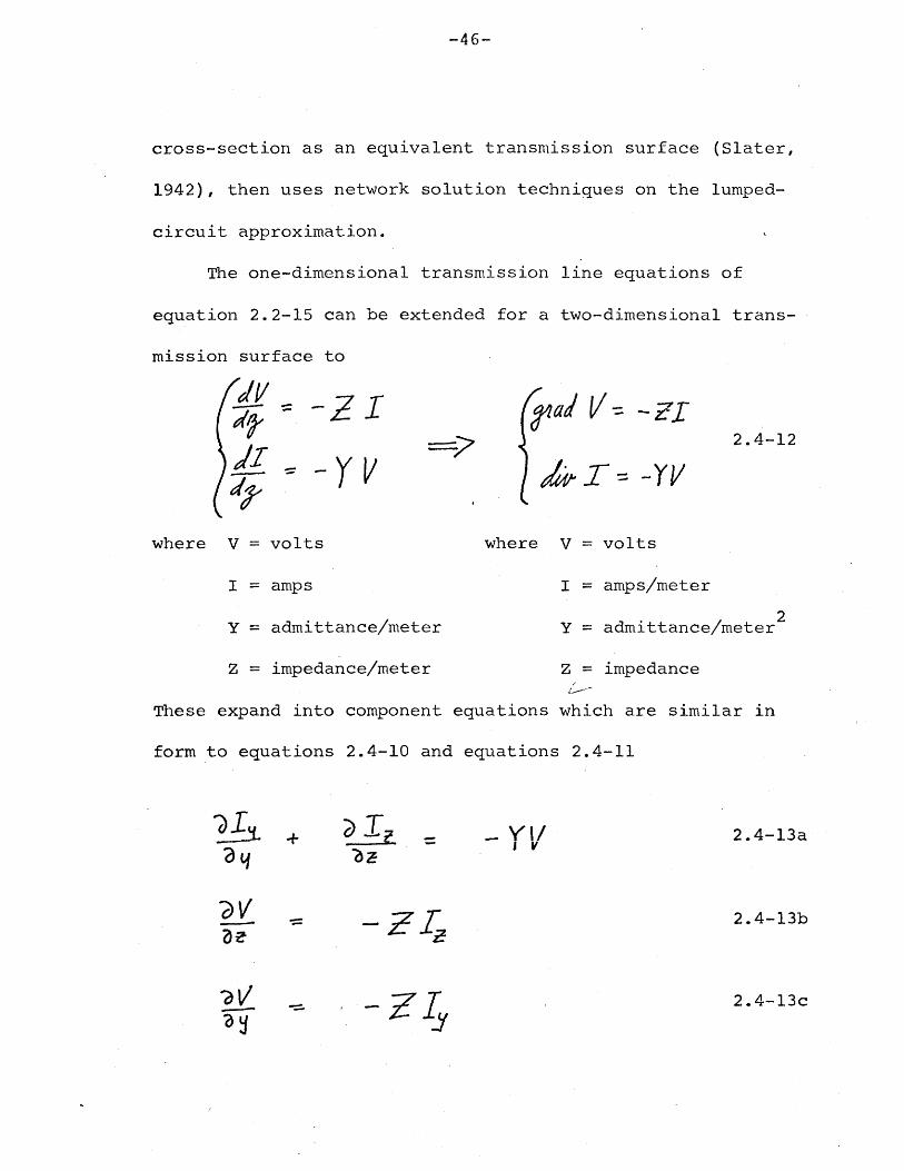
cross-section as an equivalent transnlission surface (Slater,
1942), then uses network solution techniques on the lumped-
circuit approximation.
The one-dimensional transmission line equations of
equation 2.2-15 can be extended for a two-dimensional trans-
mission surface to
J[I -2 I fad V -:: -ZI - -::: at jI -;/ 2.4-12
-::: -yv kI---YV -d? where V = volts where V = volts
I = amps I = amps/meter
admittance/meter admittance/meter 2
Y = Y =
Z = impedance/meter Z = impedance / L.--~--
These expand into component equations which are similar in
form to equations 2.4-10 and equations 2.4-11
';)I:L + () I Z -:: VII 2.4-13a
Ot.f O~ , v
"C)V - -ZI 2.4-13b ar 2
oV -::::. -ZI 2.4-13c -a~ :J
Page 59
-47-
The necessary associations are motivated by noting that for
each polarization one field component is linearly polarized
in the strike direction, so it can be represented as the'
scalar quantity in the network - the voltage.
For the E perpendicular case, the energy conservation
condition requires
-- 2.4-14
VI~ LYi! :: +Ez H)( LlX Llc 2.4-15
The associations are
Ej -<===-> 12' Et <=> I 'j
2.4-16
Hx <=== > V where AX can be absorbed by making all parameters per
unit length in the strike direction. Note that the com-
ponents of E are equivalent to different geometrical
components of I. The distributed parameters are obtained
by comparing equation 2.4-10 and 2.4-13, as
z- u(I-i-) 2.4-17 .
y -l~
Page 60
-48-
This represents a transmission surface with resistive
impedances between nodes and capacitive admittances to
ground.
For the air, the distributed impedance is zero since
the conductivity is negligible. Therefore, the voltage
must be constant along the line in the network representing
the earth's surface. This restriction on the network is
consistent with the H ~ constant boundary condition. x
The H perpendicular polarization network is character-
ized by the following associations and distributed
parameters
plus
Ex <==-> 1-/1( <=:::::-I J <:" ::::::::. > 17z.
y
This represents a transmission surface with inductive
2.4-18
2.4-19
2.4-20
impedances between nodes and resistive admittances to ground.
Therefore, the equivalent networks for the two polarizations
are both low-pass systems as required by electromagnetic
pr9pagation in the earth.
Page 61
-49-
Because long horizontal'wavelengths were not indicated
in the observed fields, k = 0 was assumed in the calcux
lations.
Although the E parallel expressions appear to resemble
those for the E perpendicular polarization, significant
difficulties arise in applying boundary conditions. Whereas
in the E perpendicular case the air above the earth could
be ignored because of the infinite impedance contrast, in
the E parallel case the air layer is mode led by a sheet of
inductances and the currents couple across the boundary.
The horizontal magnetic field in the air is independent of
the conductivity of a layered earth. Moreover, for an air
layer sufficiently thick, any perturbations in this magnetic
field component caused by two-dimensional conductivity
structure are smoothed out by the Laplace equation solutions
for the air layer. Thus, because it is constant far from
regions of laterally inhomogeneous conductivity structure,
the horizontal magnetic field can be thought of as a source.
In other words, the air layer of inductances must be thick
enough to present a constant impedance to the source.
Network solution fbr theoretical apparent resistivities
To form a network, the two-dimensional earth model must
Page 62
-50-
be sectioned into a grid of rectangles and the lumped
circuit parameters must be determined. The ~rid spacing
must be chosen smaller than a wavelength within each block,
as discussed in Appendix 1. Note that this spacing re-
striction changes with each frequency considered. Although
this restriction would appear to limit the complexity of
the model, the long wavelengths in air allow the air layer
to be modeled by only a few thick spacings, and the use of
logarithmically increasing spacing with depth allows one
model to be applicable for a wide range of frequencies.
Since the lumped impedance is proportional to the
distance between nodes and inversely proportional to the
width of surface associated with the nodes, the vertical
and horizontal impedances will be different for arbitrary
grid spacing. The lumped admittance is proportional to the
area of surface. These parameters are defined as
ZV;i:: Z Al, /b'jj
" 2.4-21 vertical impedance,
horizontal impedance, ZHjj == Z A'jj/6~i 2.4-22
admittance, Yij =: Y A!fj 6'li 2.4-23
where = distributed parameters
= vertical spacing between nodes
= horizontal spacing between nodes
i = 1, .•. ,N j = 1, •.. ,M for an N by M grid
Page 63
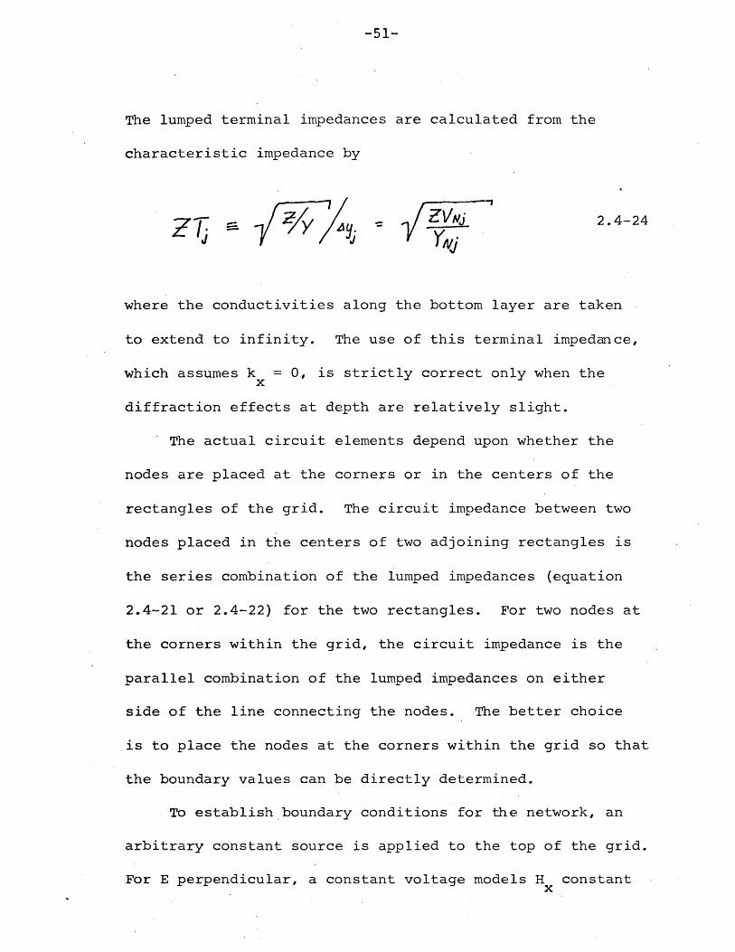
-51-
The lumped terminal impedances are calculated from the
characteristic impedance by
ZT J 2.4-24
where the conductivities along the bottom layer are taken
to extend to infinity. The use of this terminal impedance,
which assumes k = 0, is strictly correct only when the x
diffraction effects at depth are relatively slight.
The actual circuit elements depend upon whether the
nodes are placed at the corners or in the centersof the
rectangles of the grid. The circuit impedance between two
nodes placed in the centers of two adjoining rectangles is
the series combination of the lumped impedances (equation
2.4-21 or 2.4-22) for the two rectangles. For two nodes at
the corners within the grid, the circuit impedance is the
parallel combination of the lumped impedances on either
side of the line connecting the nodes. The better choice
is to place the nodes at the corners within the grid so that
the boundary values can be directly determined.
To establish ,boundary conditions for the network, an
arbitrary constant source is applied to the top of the grid.
For E perpendicular, a constant voltage models H constant x
Page 64
t.
-52-
at z = O. For E parallel, a constant vertical current
models H constant at the top of the air layer. A oney
dimensional transmission line problem was solved for both
sides to obtain voltage boundary values to force upon the
two-dimensional solution. Therefore, the ends of the model
should be far enough away from the non-horizontally layered
features so that the impedance is isotropic.
For a numerical solution, the equation of current
continuity
~ejJh6011itJ - Vz/ Z fOUflJ UtJ
2.4-25
produces a (MxN) x (~~N) coefficient matrix which is a very
sparse, diagonally dominant, normal matrix. Relaxation
techniques can be applied to such problems, but the theory
is not developed for this case where the coefficient matrix
is non-Hermitian. Although the relaxation solution will
converge, the eigenvalues of the coefficient matrix are
complex 'and the over-relaxat'ion parameter for the optimum
rate of convergence must be determined empirically. However,
a direct solution for such coefficient matrices, which does
not involve a (MxN) by (MxN) matrix inversion, has been
developed by Greenfield (1965) and was used in this thesis.
Page 65
-53-
computational details are included in Appendix 3. Finally,
theoretical apparent resistivities at the earth's surface
are calculated from the solution values of V and I using,the
appropriate associations.
Example - theoretical apparent resistivities over a vertical
contact
Figures 2:5 and 2.6 show theoretical field relationships
for the simplest two dimensionality, a vertical contact,
calculated for the equivalent networks for the two polari-
zations. The behavior of the apparent resistivities is
consistent with the earlier qualitative discussion in that
the E perpendicular apparent resistivity includes a dis
continuity of (6;/(f.)2 and the E parallel results are ~
continuous. Note that the E-H phases do not vary markedly
o from -45. Greater phase shifts result where the apparent
resistivity is a more rapidly changing function of frequency,
as is the case for large conductivity contrasts in hori-
zontally layered media.
Figure 2.5 compares the results of the network solution
with the analytic solution of d ' Ercevi11e and Kunetz (1962)
for the E perpendicular polarization over a vertical contact
with a 100:1 conductivity contrast.
Page 66
--- 1c--~ _____ _ --p,= 10 ... ...
-54-
,., \
~ \ \
... le - ~ - ~)( - _ )C ____ _
---k-- --"--. ---------IeofJ-f~:-; 1000 •
500
I ------··--·--------------10·
• Net~:lork res ul ts
x Analytic results
'---:--______ .l._. _______ . __ &...-....-_____ . ______ ......J..._~ ______ _1__.. __ ._
~
60 30 0 30 {'o
Distance in kilometers
x-~ /' \ . \ ..,- X I
'1:/ \ ,.,.. \ -- \ -----,:
,.-
... ~~-- * - *- - - '*- - -- - -
Figure 2.5 Comparison of theoretical apparent
resistivities calculated by network solution and
by analytic solution (dF.rceville and Kunetz,1962)
over a vertical contact. Conductivity contrast -3 -
is 100:1. Frequency is 10 cps.
-6StJ
-SS"-
- ~ - ~~
ID Ul co
..c::: C4
Page 67
Conductivity model
-3 For frequency = 10 cps
Apparent resistivities
/
-55-
.,.- .::? X --__ -- _ .Y
l5Ir~_K_H _______ /~OD ________ ~~~O ________ -1~~w===~~======~~~O====~~/~OKfl lOO
~0 e--,e,if
e E PFlRRLLeL ~ E. PERPENJJ/('ULRR
'E-H phase r-__________________________ ~v~._----------------------------~-SSD x.... .,.
/ x <:) ----0 _______ . ___ x , eJ,0- ~ 0_
~---------~---.-- ~ --0 ~t!PC}x-)C-x-,,- -". ~-
------ (i)- 6)" eG
----------------------------~ ____________________________ ~_3S4
H vertical/Hy
Hy (relative to value far from contact) r-------------------------------~-------------------------------J,lO
/./0
. e.......c>0 ______ 0~ ~~
e e 1----------- e , E>_e_ E> -. ----0---- 1.00
--------------L---------------L·O.90
Figure 2.6 Theoretical magnetotelluric field relationships over a vertical contact.
Page 68
-56-
¥igure2.6 shows the the()retica,l, apparent resistivities,
the E-Hphases, the ratio H vertical/Hy' and the variation
of H over a vertical contact with a 10:1 conductivity cony
trast. The skin depth appropriate for each side is included
to indicate its usefulness as a IIrange of influence"
-- parameter.
-'-. The variation of the Hvertical/H perpendicular ratio
is the magnetic induction method indication of a lateral
contrast in conductivity. Note that the delineation of the
,-- contact is much better defined by the E perpendicular
apparent resistivity. Moreover, this variation, for a
ocean-continent boundary model, exhibits the well-known
, .. coast effect of a . more extensive H vertical/H perpendicular
anomaly over the resistive (continental) side.
The variation of H perpendicular over the contact is
plotted to show the relatively small variation in the
magnetic field over a laterally inhomogeneous conductivity
structure. It should be emphasized that the two lower
curves, for H vertical and H perpendicular, are for the E
parallel polarization only; the magnetic field is constant
for the E perpendicular polarization.
Page 69
-57-
2.5 Properties of the magnetotelluric impedance tensor
To explain peculiar magnetotelluric field results in
which the Cagniard apparent resistivities are not inde-
pendent of the measured orthogonal fields or the time of
measurement, the impedance must be expressed as a tensor, as
formulated by Cantwell (1960):
2.5-1
The admittance formulation, defined by H. = Y .. E., is ~ ~J J
mathematically equivalent to the impedance formulation, but
the impedance is more commonly used because the more uniform
magnetic field can be thought of as a source.
Therefore, the electric field in one direction may
depend on magnetic field variations parallel to, as well as
perpendicular to, -its direction. Therefore, "Cagniard
apparent resistivities!! calculated from raw ratios E /H ~ y
or E /H can vary with time as the polarization of the y x
source field varies. As long as the source field wave-
lengths are sufficiently long, however, the tensor elements
should be time-invariant.
Since Z12 and Z21 can be calculated for a given two-
dimensional conductivity structure, magnetotelluric data
Page 70
-58-
can be interpreted quantitatively if the geologic structure
involved is two-dimensional and if the elements for the
tensor alligned with the structure can be calculated from
the data. A structure can be considered two-dimensional if
a conductivity cross-section is constant along a strike
direction fora distance much longer than a skin depth.
Therefore, two-dimensional tensor impedance analysis
of magnetotelluric data consists of three steps: first the
calculation of the impedance tensor with respect to the
measuring axes, then the rotation of this tensor into the
principal axes, and finally, the comparison of apparent
resistivities calculated from the rotated tensor with
theoretical two-dimensional results.
Properties of theoretical impedance tensors
Properties of theoretical impedance t'ensors can be
obtained through matrix analysis. Complications arise
because Maxwell's equations couple together the orthogonal
components of E and Hand, hence l the off-diagonal elements
are the dominant ones.
For a cartesian rotation, when the new axes are rotated X
degrees clockwise,
~ .... ---~~ .... ...... ..... .... ...... ~'
Page 71
-59-
the transformed field components are
E'= lE /I' = jf !I 2.5-2
where
1= et;trj; ~f ] 2.5-3
-SIM ~ tJJtP
To transform the z tensor, such that
2.5-4
then Z· must satisfy
2.5-5
or
2.5-6a
I
z,~ -;~3.(glp + (z;l~-Z,J,4Wf~f -~I siafl 2.5-6b
I
.0, -; ~I t)tl-tf f (~;z -~J Ui/ Ct2/ - Z/:l. si« 'I 2.S-6c
I .
Z:!.;l-:0.? tdt 15 - (0~ fZJ ,atit/~ l' ~I SUl<-, 2.S-6d
Page 72
-60-
For an isotr~pic or a layered earth,
2.5-7
)
Then upon any rotation
I I
2;/ ~~ - ~:z. .i!:ll = )
2.5-8
Z/ - Z;Z; - 0 -This indicates the known result that for the isotropic earth
case there are no E H or E H terms and the impedance is x x y y
independent of the orientation of the measuring axes.
For a two-dimensional earth with the m'easuring axes
alligned with the structure, the impedance tensor is
characterized by
Z/( :: Z;J2. :::: 0
Z/?, ~ ~:<I
2.5-9
The structural strike and the perpendicular direction are
defined as the principal axes of the conductivity structure.
Upon rotation away from the principal direction, equations
2.5-6 indicate that diagonal elements appear, but such that
I
~I /
- Z:?~ 2.5-10
Page 73
-61-
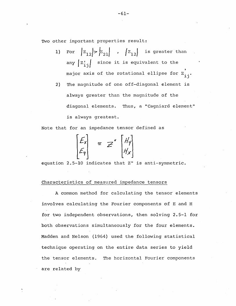
Two other important properties result:
1) For I Z12J"7 f21/ is greater than
any IZij! since it is equivalent to the
major axis of the rotational ellipse for Z ... 1J
2) The magnitude of one off-diagonal element is
always greater than the magnitude of the
diagonal elements. Thus, a "Cagniard element"
is always greatest.
Note that for an impedance tensor defined as
equation 2.5-10 indicates that ZII is anti-symmetric.
Characteristics of measured impedance tensors
A common method for calculating the tensor elements
involves calculating the Fourier components of E and H
for two independent observations, then solving 2.5-1 for
both observations simultaneously for the four elements.
Madden and Nelson (1964) used the following statistical
technique operating on the entire data series to yield
the tensor elements. The horizontal Fourier components
are related by
Page 74
-62-
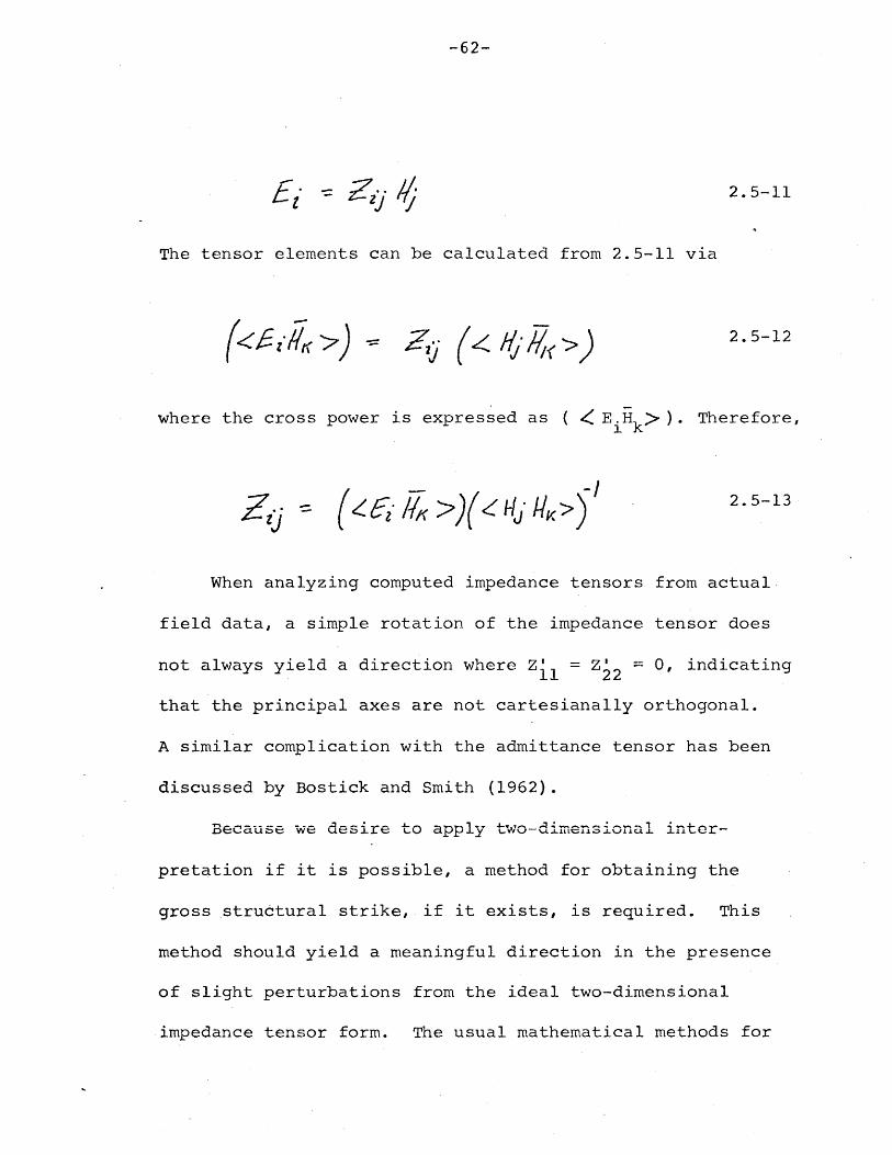
2.5-11
The tensor elements can be calculated from 2.5-11 via
2.5-12
where the cross power is expressed as ( < EiHk> ). Therefore,
2.5-13
When analyzing computed impedance tensors from actual
field data, a simple rotation of the impedance tensor does
not always yield a direction where Zil = Z22 = 0, indicating
that the principal axes are not cartesianally orthogonal.
A similar complication with the admittance tensor has been
discussed by Bostick and Smith (1962).
Because we desire to apply two-dimensional inter~
pretqtion if it is possible, a method for obtaining the
gross structural strike, if it exists, is required. This
method should yield a meaningful direction in the presence
of slight perturbations from the ideal two-dimensional
impedance tensor form. The usual mathematical methods for
Page 75
-63-
obtaining principal axes of an arbitrary complex matrix
yield complex skew eigenvectors. The two following
physical criteria yield conceptually simpler directions:
(1) the direction where an off diagonal element is
maximum; and" (2) the directions where a linearly polarized
H produces an E in only theorthogonal direction. These
criteria, which are discussed in Appendix 4, are incorpo-
rated into the data analysis described later in this thesis.
To determine whether two-dimensional interpretation is
even possible, a IJtwo-dimensionalitylJ measure can be con-
structed from the elements of the impedance tensor. From
equations 2.5-6, the following expressions are invariant to
rotational transformations:
I I
Z/( + Z:l:J. z,,' -- Z;.',
;:::. Z,/ + Zll~
~ Z,z. - 'Z/ll
From 2.5-10, the sum , I
-::2 + J should vanish for an ideal ~II ~,.'l~
two-dimensional impedance tensor. By normalizing this sum
I I
Z/2 -C~I , the invariant ratio by
2.5-14 I
~I
Page 76
-64-
essentially measures the skewness of Z· [ °1 -0'] and is a
J.,lseful "two-dimensionality coefficient".
Improper impedance tensors from finite-length dipoles
Severe departures from two-dimensionality cannot be
analyzed quantitatively because solutions of the three-
dimensional forward problem are presently unavailable. A
more fundamentel problem lies in measuring the electric
field with a dipole of finite length. For a one-
dimensional conductivity structure with k = 0, the surface x
electrical field has a potential and the measured voltage
is independent of the connecting cable. For a two-
dimensional conductivity structure, not only is the surface
field non-uniform, but the' equipotential concept is not
valid and the voltage measured between two electrodes
depends upon the location of the connecting cable. This
latter complication is due to the fact that E is not curl-
free and the associated vertical magnetic field contributes
a voltage from Faraday's Law
2.5-15
To calculate, the possible contribution from this
integral, consider the following configuration:
Page 77
-65-
The" electric field contribution is
For
and
Erlta) - /z! -::: I'UJIIc. ~ -
~ :z. n
Hi!~: t H;)"l-an area with - R -with
H
X " A~ being times a skin depth J
£(1/1) ; ~ l? (/{/ +Iq ) ${ X ti!i. ~ -6 R X (#. HlwtisdJ)
::: k f< X ( £ MtfJJ )
2.5-16
11
o-/-A7 - I'(,IJ~
2.5-17
Therefore, the contribution from equation 2.5-17 as a per
cent of the horizontal electric field ( iE: JA-) is RX/{i ~~lf'
For example, over an area where the H vertical/H horizontal
ratio is 0.2, the cable should be less than two thirds of a
skin depth away from the straight line between the electrodes
to keep this contribut"ion less than 10%.
Even with straight dipoles, the measured potential dif-
ferences represent integrated electric fields corresponding
to an average of the impedance tensor along the dipole.
Page 78
-66-
Thus, in.:using 50 km electrode spacing at right angles, one.
dipole can s-pan an area characterized by one Z while the
other dipole spans another area 30 to 40 kms away charac-
terized by a different z. To obtain less distorted results,
crossed dipoles should be employed:
v x standard crossed
with the available electrode connections restricted to
existing telephone lines, crossed dip91es could not be used
in this thesis.
The measured tensor relationship is
I~] In,~t.irlf - SII?I si-Lf
( fBn ~ fs,J SVA 9 m 2.5-18
where A .. and B .. are the elements of the tensor referenced 1J 1J
to the strike direction appropriate for dipoles
A and B
f is the angle from A to principal structure axis
Upon rotation of the tensor into the structural axes, the
tensor is
(SBz, -St1ZI)Si«~~ S BZJ fA£"<} r J n ",sk).,p
2.5-19
Page 79
-67-
This same tensor would result if the measured E field had
been rotated first into the strike direction. Note that
the diagonal elements do not vanish unless A .. = B ..• 1J 1J
Expression 2.5-19 was evaluated for theoretical.
values of A.. and B.. ·(obtained by the methods of section 1J 1J
2.4) for various locations over a vertical contact with a
100:1 conductivity contrast. Although two-dimensionallY7
improper tensors (Zll ~ - Z22) were obtained for almost
every measuring orientation, only when the dipoles were
spanning opposite sides of the contact were the skewness
coefficients large and the calculated apparent resistivities
and principal direction inco~rect~ Figure 2.7 includes
some numerical results.
These theoretical improper tensors afford an empirical
check on the skewness coefficient of equation 2.5-14. For
values of the skewness coefficient less than 0.3 the cal-
culated principal directions are good to within 10 degreesj
for values greater than 0.6 the calculated principal
directions are meaningless.
Page 80
El.
Ell
-68-
Example: vertical contact -3 f:: 10 ___ ~ps
f, -:: 10
Theoretical apparent resistivities:for small dipoles:
_5"1/" .. 57 0 _,~O _'30
1.0 8.a 6.9 5.fJ
-320 .. 3.1 0 -3~o _33' 16 17 ~o JJI
, I
I/O ~o
J..' .. ,,0
_J'o -'ISo 30
_1/50 -lIsO 133.0
·11>0 (,7
lI?b
-SJ() n
I
~o
... 1/40 -f/J!0 -'11'0 J17f) //~ //J.a
_s,O /11) /36511> /r,isao
For 30 km dipoles oriented at 4S0 to strike: ~
~ I
30 «11
Observed apparent resistivities: T£IJSOi.
9 .. 33 0 .y 520"I/.~O <r '3 IffIAnCAJ(
,10 12~/S1J{J/77€5
7"~'o -37· I~ /flDN(,
<- f,(/IJClpAL 3.¥ IfX£5
£ .. w #~,oE ~ Principal axis
O.Df 0,66 ~ Skewness coeff.
F:i9'ure 2. 7 Bffect of finite-length dipoles on the
measured apparent resistivities over a vertical contact
Page 81
-69-
Chapter 3 - Magnetotelluric Experiment in the Southwestern
united States
During the summers of 1965 and 1966, a magnetotelluric
survey occupied stations mostly along a profile from Yuma,
Arizona, to Roswell, New Mexico. The recording sites are
shown on a location map (Figure 3.1).
This chapter discusses the acquisition, analysis and
interpretation of magnetotelluric data from these seven
stations. This treatment incorporates many features not
included in the initial approach by Cagniard (1953), namely,
the use of magnetic data from one observatory for a number
of distant telluric measurements, the use of forty mile
telephone lines for electrode connections, the use of a
tensor approach for calculating apparent resistivities, and
the use of two-dimensional interpretation.
3.1 Magnetic field data
To sample upper mantle conductivity, electromagnetic
variations with periods greater than one hour are required . ....-----
The Tucson Coast and Geodetic Survey Geomagnetic Observatory
routinely records normal magnetograms which include this
period range. Since the entire region of interest in the
Southwest lies within 400 miles of Tucson, the uniformity of
Page 82
CALIFORNIA
/
\~ \
ARIZONA NEW MEXICO
® . -Gallup Santa F~
<lhoenix
@f Roswel
@. e ®~Tucson Saf IO~d @ •
Deming __ ----__ ~[.r~E--l-P-a-s-o-A
~-----------~~ ~
MEXICO Figure 3.1 Location map
~ Te11u~ic recording sites
A Geomagnetic stations (Schmucker,1964)
I .....]
o I
Page 83
-71-
the magnetic field suggests that the.magnetic field observed
at Tucson could be used as being representative of· the
entire region. This strong assumption requires the hori~
zontal wavelengths to be very long. Thus, a correlation
study of geomagnetic observatory data from a few stations
provides observational evidence of the horizontal wave-
length structure to justify both the use of only Tucson
magnetic data and the assumption of a plane-wave incident
field in later interpretation.
In Figure 3.2, the magnetic observatory data from
Tucson and Dallas, stations 800 miles apart, are plotted
together for comparison for two time periods of six and
four days.' Observatory data from Boulder, Colorado, appear
to be similarly correlated with the Tucson and Dallas data.
The correspondence between the data shown in Figure 3.2 is
striking; the diurnal variation shows a phase shift ap-
propriate to the lateral separation of the stations, the
higher frequency variations appear to be simultaneous.
The results of a quantitative correlation study of the
magnetic field components at Tucson and Dallas are shown in
Figure 3.3. Coherency, phase shift, and power
(Dallas/Tucson) are plotted as a function of frequency for
the two horizontal components. The shortest horizontal
"
Page 84
t.f) <.D m
, Z CIO
CIZO ~-OZ:
/ er: r,,~ O·--.r-a-~
r-er: I a:: AC'J uz ....... ~U er: l{"")W
>UZ IT-=:)--:J UJI- -, (jl
m u
U(f) ,--,a: r-Xlf1 lJJW(O z~m ('J - ....... aV) " LITm CLJ I lJj -.JtD ou:
DW Z -_:J J
H \./ DRL r::-::: ~ __ ------======-o::::::::=----=:::::::::::::====:-=::::::====---------::::::::::==:::::::=---------::=:::::::::=_====:::::::::::::::::::.:.::-~7"-:::::::::::::'-~/'::::::'=~=:::~::::=::::::'-::":>_.....,c.;~~~:l<t.rI __ -r:1V_,...-.J.c~. ,\ TUC ==-=- ---=--==--_"",,-;;::---:::"'-" ------=::::::::==========-=.:-=-~~=-:==::::::::=-:.:;:--~./--------------..:--==-':::--:-.-:.:---:....:-:-=--=-=--=--~---- - --" ---- --"",,~---- ----=:." .---- -~} =< C>-
Hy ORL TuC
~PMMR /INCH GPMMQ /INCH
Figure 3.2
"'.-- -- ----"'--,
Geornagnetic Observatory Data
Dallas, Texas, andhTucson, Arizona
------ -.--....---.- ." --- -'
11 ,~"
I -.J N I
Page 85
-73-
1 day 12 hour period 1 hour
-:..- ... .0 -5 10
90
60
30 - j-t- ;
. ,
- t . t + ...;. - ~ .. ~
-60
---T----;'- ,-r---- +- ~ "j --j _-r L -~-t
"~ •• ,i-·I'·-'I ~r:-~-~ ; · + -~-- -..--.. t--
r ... -... ·
-4 10 cps
PO\Jcr ratio Dallas/Tucson
... ~ + ~ r
~. T ·-r r---l ....
Phase shift in degrees (Tucson relative to Dallas)
• 7 5 ~-+-+--..;.-+-....... -+-.. +
=Lf--:~_ -t--~-t'
- j- 1"- +- ...
• 50 -5 10
-r--r--"-i r to ..... l ~ .
Figure 3.3
Coherency amplitude
C?herency analysis of magnetic fluctuations,
Dallas and Tucson data,June 12-17,1965
20 rnin
Page 86
-74-
wavelengths suggested from these results are about 10,000
km for the high frequency end. The diurnal phase shift
represents a true delay with a horizontal wavelength of the
earth1s circumference. The higher frequency phase shift
could be expla'ined by a 2.5 minute delay due to an ac
counting error, since the digitizing sampling rate was 2.5
minutes. The power ratios vary over a factor of two, but a
'single total horizontal component ratio would be signifi
cantly flatter.
The flat power ratio and low phase shift, together
with the high coherency, validates the long'wa~elength as
sumption. It .should be emphasized that this amplitude
correlation between magnetic fields from two separated
observatories does not apply to the vertical component,
which is far more sensitive to the subsurface conductivity
structure.
The major benefit of using the Tucson magnetic data
is that only the telluric measurement had to be made. The
magnetic data was recorded on well-calibrated variometers
and was digitized by NASA. Thus, digitized magnetic data,
sampled every 2.5 minutes, consisting of H (magne~ic
intensity) in gammas and D (magnetic declination) in tenth
minutes, was available for use in the magnetotelluric
investigation.
Page 87
-75-
Sources of the incident magnetic field
The magnetic field data plotted in Figure 3.2 clearly
represent two source mechanisms, the diurnal· variation and
magnetic storm activity. Detailed discussions of these
mechanisms are found in Chapman (1·964) and Paghis (1965),
for example.
The magnetic diurnal variation is caused by the dynamo
current system in the E-layer of the ionosphere which is
set up by solar heating of the day-side ionosphere. For
Tucson at the summer solstice, the horizontal component of
·the diurnal variation is~. roughly. elliptically polarized with
a major WNW component and rotates in a clockwise sense.
Magnetic storm activity is directly correlated with the
bulk velocity of the solar wind (Snyder, 1963), and is
ul~imately due to enhanced particle emissions from the sun.
The enhanced solar wind perturbs the entire magnetosphere
so that disturbances, which propagate down through the iono
sphere as hydromagnetic waves, occur nearly simultaneously
over the globe. The major characteristics of a magnetic
storm are well shown in the. June 12-17, 1965, data of
Figure 3.2. The sudden commencement, the sudden increase
in the field, is due to a sudden increase in the solar wind
pressure which causes·a compression of the magnetosphere
Page 88
-76-
and the field lines. The later main phase, the extended
decrease in the field, is due to either the ring current
drift of energetic particles in the magnetosphere or
transport of field lines into the tail. other sources of
low-frequency fluctuations are ionospheric currents
induced by electric fields associated with disturbed
magnetospheric plasma. Isolated "bay" variations are
caused by solar-flare induced, temporary enhancement of
polar D-Iayer ionization.
Although these mechanisms produce long horizontal
wavelengths at low latitudes, the polar and eq~atorial
electrojets plus increased over-all activity in the auroral
regions are more local sources with shorter horizontal wave
lengths. Magnetotelluric investigations in these regions
must consider the finite source length (Spitznogle, 1966).
Page 89
-77-
3.2 Electric field measurement
For the low frequency range investigated in this thesis,
the skin depths are large (50-500 km) and the associated.
electric fields at the surface are weak. Large electrode
separations in the measurement of the electric field are
required to average out the irregularities in the surface
conductivity structure in order to unmask the effects of the
deeper features of interest. Telephone lines, which have
been used occasionally (Rooney, 1935), provide such large
separations. The stations shown in Figure 3.1 are those
locations between southeastern California and the Texas pan
handle where it was possible to obtain two long telephone
lines at approximately right angles. For many of these
electrode configurations, local crustal structures, particu
larly sedimentary grabens, are the same scale as the dipole
length. Therefore, the electrode separations are not long
enough to average out the surface condu~tivity variations.
As discussed in section 2.4, this situation may result in a
distorted measured field. Data from additional stations at
El Paso, Texas, and Santa Fe, New Mexico, were corrupted by
commercial noise.
At· each station, all-metal land lines without
intermediate-stage amplification and filtering carried the
Page 90
-78-
signal from the electrodes into the central telephone office
where the recording equipment was kept. Lead plates, 6" by
8" in size, buried about three feet in moist sandy soil,
provided electrode pairs with resistance usually less than
600 ohms. The telluric lines were from 16 to 85 kilometers
in length. Typical measured voltage fluctuations of 0.1
volt are well above the low lead-electrode noise levels.
The recording instrumentation consisted of a variable
gain amplifier incorporating a two-pole low pass Chebyshev
filter (E = 0.25) and three Rustrak recording voltmeters for
each channel. Amplifier response is given in Figure 3.4.
To allow unattended recording, two recording voltmeters, at
3"/hour chart speed, were of different sensitivities (1 and
5 volt full scale) to record large variations in rms
amplitude. The third recording voltmeter (5 volt full
scale) ran at I"/hour chart speed to provide a monitor
recording for comparison with the magnetograms. Table 3.1
lists the recording details - recording dates, electrode
sites, dipole lengths, and gain settings.
The data were hand digitized at a 2.5 minute sampling
interval to'correspond to the sampling interval of the
magnetic data. Orthogonal north and east components of
the telluric field were calculated from the non-orthogonal
Page 91
~79-
1.00
0.10
0."01
12cf
10 10
Figure 3.4 Gain response of telluric instrumentation
Page 92
Gain Station Recording Dates Electrode Sites Ro s we 11, """'N~ • .."-M-.-.......,6,,,.../-r::ll (7 !~) 1','="'1 )---6-:;;-7-r;1·-=7:-;('-:S:---::P~~-::"'1 )r--, --=-1-::::9-::6=-=S=-----Cc=-r-o-u-n-a=-:1' -a-t..,.---=R-o-s-"-le.....,l=-l=---..,-t-e-=l-e-p ....... h-o-n-e--o-::f~f::""'li.-c-e-----
Deming, N.M. 6/7(S PN)-6/14(4 PH), 1966
Safford, Ariz. 6/26{noon)-7/5{9 PM), 1965
Tucson, Ariz. 6/15 (noon)-6/27 (noon) , 1966
Phoenix, Ariz. 7/6(9 PM)-7/23{2 PM), 1965
6/28{1 PM)-7/21 (noon) , 1966
Yuma, Ariz. 6/5(6 PH)-6/10(9 AM), 1965
Gallup, N.M. 7/22 (9 lV1) - 8/1 (9 AM), 19 6 6
Hondo, N.M., 71.6 km to N88°W Artesia, N.M., 63.S'km to SlloE
Ground in Wi1na, N.M. Silver City, N.M., 62.8 km to NloE Deming, N.M., 49.9 km to N85°E
Ground at base of Swift Trail Rd. Pima, Ariz., 20.8 km to N34°W Morenci, Ariz., 24.1 km to N66°E
Ground at Fort Lowell Ruins, Tucson Red Rock, Ariz., 48.3 km to N52°W Sahuarita. Ariz., 35.4 km to SlOoW
Ground at Surprise, Ariz. 'Litchficld, Ariz., 16.1 km to S16°N Apache Jet., Ariz., 73.4 km to S75°E
Ground at Maricopa, Ariz. Sun City, Ariz., 69.2 km to N23°W Apache Jet., Ariz., 61~2 km to N46°E
Ground at Yuma telephone office Somerton, Ariz., 20.7 km to S38°W Ligurta, Ariz., 29.9 km to S79°E
Ground at Gallup telephone office Newcorob, N.l1., 85.3 km to N3°E Thoreau, N.¥.,51.6 km to S77°W
Table 3.1 Telluric Recording Data
7.9X 10.5X
20.0X 20.0X
2S.4X 27.0X
20.0X 50.0X
l8.3X 7.3X
20 .. 0X 20.0X
11.SX l5.5X
20.0X 20.0X
I co 0 I
Page 93
-81-
measurements by
where
E)( "'- (It COt- f5 - E siJP() ! fM, ( 0<. -p) E~ = (11 s#t~ r B~ 0(.)/ ~ (""-f)
3.2.1
Page 94
-82-
3.3 Method of data analysis
Spectral and coherency analysis were used to reduce
the magnetotelluric data of this thesis through computer'
programs written by T. R. Madden and the author. Spectral
analysis of low-frequency electromagnetic data has been
discussed by Madden (1964).
Two separate analyses were applied to the data, in
-5 which the frequency content ranges from the diurnal (10
-2 cps) to ·the Nyquist (.33 x 10 cps). For the higher
frequencies, a digital-sonogram analysis results in power
spectra, coherencies, impedance tensor elements, and
apparent resistivities as a function of time. Hopkins and
Smith (1966) have also presented running power spectra as a
part of magnetotelluric investigation. For the lower
frequency decade, the typical six-day data series is not
~ufficient for a meaningful running spectral analysis.
Moreover, for the low frequency energy, which is dominated
by the harmonics of the regular diurnal variation, the lack
of random signals produces a high H H coherency which x y
causes the tensor elements computed from equations 3.3-3 to
be unstable. Therefore, the data were rotated into the
principal directions, as determined by the higher frequency
analysis, before spectral computations.
Page 95
"-83-
To calculate power spectral estimates of magneto-
telluric data Cantwell (1960) and Ellis (1964) assumed
stationary data series and calculated power spectra by
Fourier transforming the auto- and cross-correlation
functions. An alternate approach to the calculation of
power spectra, which is particularly efficient if many
inter-related cross-spectra are desired, is through the
Fourier spectra of the individual data series:
Fourier spectra: £X((JJ) I £y(w) ) JIx(W} ) IIy (tv)
Power spectra: <Ex Ex > , ef~.
Cross spectra: < E)< Hr:> ) ek.
where . Ex /w) J etc. = conjugate Fourier spectra
and the brackets represent averaging in time for finite
band-widths. This scheme substitutes computationally quick
multiplications for time-consuming correlations and was
used in both approaches.
gigher frequency analysis
For frequency components between 1.1 x 10⁻⁴
cps (2 1/2
-3 hours) and 1.7 x 10 cps (10 minutes), the four data series
were high-pass filtered, then fed continuously into a bank
of twenty constant-Q digital recursive filters spanning the
frequency band. Constant-Q filters, which measure power
Page 96
-84-
density as power per octave, effectively "flattenll
geomagnetic power spectra with rough l/f characteristics.
The filter outputs were corrected for recording instru-
ment response (for E and E ), plotted as single frequency x y
polarization ellipses for the electric and magnetic fields,
and then used to obtain the following auto-power and cross-
power spectra as a function of time within the data set.
Cross spectra: -<ExEy > J
< 6~ H/;>}
Computational details, including a more specific des-
cription of the filters, can be found in Appendix 5.
These spectra were used to calculate coherencies,
which are required to calculate the impedance tensor
elements where:
coherency (AB) = 3.3-1
The coherency is a quantitative measure of the amount of
linear relationship between two data series. Thus, the
coherency measures the consistency of the phase difference
between the two data series.
Page 97
-85-
Now the impedance elements can be calculated from
equation 2.4-4
3.3-2
Expansion yields
2, -:: /£.) ( foh EX fix - fot Ex IIy Nh 11&-) 3.3-3a ---/Hxl / _ I coh Hxlly /1-
2,,, ~ /Ex/ ( ~o4 Ex fly - colt Ex I/x ech )I" IIr) 3.3-3b
/Hv l ..
/ - I cok Hx H "I L .
Z:l.1 -= /£'(1_ ( Coh 4. IIx - tbh £'1 I/~ tcA I/'t~ ) 3.3-3c
I Hr! I - /tdA I/x H'1/1-
Z:l~ -:: 1£,[' ( t~t Er lit - Cbk £'/ fix (~'!lx I!r ) 3.3-3d
/Hy/ / - I Cah Hx 11" /
where I / ( -- ] '/3-EX -= <. Ex Ex> etc., the Four ier
amplitude spectra. From these impedance elements, principal
axes and principal values were calculated using the methods
outlined in Appendix 4.
Standard Cagniard resistivities are simply calculated
from the power spectra as
Page 98
-86-
~ (fJ - a~ <EX Ex> I fl l.y -
f <H~ 1/'(>
3.3-4
Po. JX (I) - 0, :l. _ -< 6'1 Er > - f < Hx Hx> 3.3-5
where the frequency, f, is in cps, the electric power
is in (mv/km) 2, and the magnetic power is in (~) 2 . As
discussed in Chapter 2, however, meaningful apparent
resistivities for two-dimensional structures must be calcu-
lated from the principal values of the impedance tensor.
where
0.:< -f
= principal values of Z .. 1J
3.3-6
The digital sonogram analysis yields power spectra,
coherencies, and apparent resistivities as a function of
time, and, thus, exhibits the time variations of the
characteristics of the sourcerfield and the calculated
apparent resistivities. The coherency between orthogonal
E and H components: which can be used as a "reliability
criterion" for the calculated apparent resistivities over
layered-media geometries, can be deceivingly low over
Page 99
-87-
two-dimensional conductivity structures and, thus, must be
replaced by a criterion which involves all four horizontal
components. A useful measure of predictability is the
_predicted coherency between E and E;"".for the two components,
E and E . x Y
3.3-7
where 3.3-8a
and 3.3-8b
Upon expansion this expression becomes
(!oh(E{ti):: If/xl Z if eoh. (1/" Ei) + I Hy I Z'i,g CQh CH., E; ) 3.3-9
U 2';/IHx /1. + I Zi~ rl/ly t + ~ IIM/III[ / /?dli ,lit eot ~ /{yfJ'r--
These coherencies were also calculated as run~ing para-
meters.
Lower freguency analysis
To calculate results for frequency components between
lO-~ cps (1 day) and 1.3 x 10-4
cps ·(2 hours) I the data
were first rotated into the principal directions for the
measuring site as determined by the tensor analysis of the
Page 100
-88-
higher frequency analysis. Fourier transforms of the four
complete data series were calculated, then the same four
auto~power and six cross-power spectra as in the higher
frequency analysis.
Cagniard apparent resistivities, coherencies, tensor
predicted . elements, E - E coherenc1es, and principal value
tensor ap~arent resistivities were calculated using the
expressions presented above. When a high H H coherency x y
causes the tensor elements to be unstable, as is the usual
situation, the Cagniard apparent resistivities are more
reliable since the reference axes have been al1igned
approximately with the principal axes.
Sour£es of error.
Errors in the data analysis are more likely due to
bias and high sensitivity to noise than statistical errors
in the computational estimates. The. problem of estimating
the statistics of a stationary process are not applicable
since low-frequency magnetotelluric signals have transient
characteristics. The running spectra emphasize the non-
stationarity of the data. Other digital analyses of magneto-
telluric data over many decades of frequency·have pre-
whitened the data to reduce spectral spill-over (Ellis,
Page 101
-89-
1964; Hopkins and Smith, 1966). Pre-whitening, other than
the use of power/octave in the sonogram analysis, did not
improve the results in this investigation.
High sensitivity to noise in the digital data can
result from poor digitizing resolution at times of low
signal level, from calculating relatively small tensor
elements for severe anisotropy, or from calculating the
impedance elements when the' H H coherency is high. x y
Actually, the form of the expression for Z .. (Equation 1J
3.3-3) is a strong argument for using the impedance rather
than the admittance, because the denominator of the
expression for Yij
contains (1 - /coh ExEy/ 2). The pre
ferred current direction caused by two-dimensional con-
ductivity structure causes the E E coherency to be greater x y
than the H H coherency and, hence, division by x y
(1 - Icoh EEl 2) can be very unstable. x y
Bias error on the electric channels could be intro-
duced by an E field miscalibration, an inaccurate dipole
length, a non-straight telephone line connection between
electrodes, or an E field distortion. Except for stations
with very high skewness coefficients, this combined error
should be less than 20%.
Worse bias error can be introduced by the use of the
Page 102
-90-
Tucson data as representative of the magnetic field at the
telluric recording sites. The variations between magnetic
. data from Dallas and Tucson shown in Figure 3.3 are re-,
flected in apparent resistivities calculated using Roswell
telluric data and magnetic data first from Tucson, and
then from Dallas~ Apparent resistivities differ by factors
up to 2.5 but averaging 0.2, while the associated E-H
phases differ by amounts up to 700
but averaging 150
{Figures 3.9 and 3.11}. Differences between the magnetic
data are due to real changes of the field at two locations
1300 km apart at slightly different geomagnetic latitude,
plus possible high frequency contamination from different
instrument responses and digitizing and aliasing error.
Since the separation between Dallas and Tucson is more
than twice as great as the distance from Tucson to the
telluric stations, the error in using the Tucson data as
representative can be up to 60% in apparent resistivity
values and 35% in the phase estimate, but only at the
higher frequencies. As mentioned in section 2.5, laterally
inhomogeneous conductivity structure can affect the
magnetic field perpendicular to the structure. However,
this effect is less than 2% for the theoretical models
involved.
Page 103
-91-
Bias error can be introduced in the calculations by an
incorrect rotation angle for the low frequency Cagniard
estimates and by the effect of noise on the impedance
elements. To examine how added noise can effect Z,. and how
well the E predictabi1tiy coherency detects this error,
consider:
a) incoherent noise introduced on E. such that ~
E·N~ l - E'+-N 1
< Ei N > = 0
<HjA/> -0
I Ei N~ J :a C I I £i /
Then the coherency is given as
...
3.3-10
3.3-11
For coh (H H ) small, as was usually chosen, the impedance x y
elements (from.equations 3.3-3) are
z·· -tJ 1£-;1 - {'{)ft (E,l" HI) JHj/ (e v
3.3-12
Page 104
-92-
From 3.3-10 and 3.3-11,. znoisy is given as
4
3.3-13
Therefore, the impedance elements are unaffected by in-
coherent noise on the E channel •
. For coh (H H ) x Y
0, the E predictability coherency of
equation 3.3-7 reduces to
(E.pred
For noise-free data, coh E.) = 1.0; for noisy data, 1 1
from equation 3.3-11,
3.3-15 ~I
Thus, a E. predictability coherency of- 0.8 can be explained 1
by 25% added noise power to E .• · 1
b) incoherent noise introduced on H. such that J
H·NDw, J H: + N
"J
<.£;N-:> - 0
~HjN> - O.
I H.IJ~I =- COl. I Hj I J.
3.3-16
Page 105
-93-
The effect on the coherency is
IJ· ) eoh (ti IIj ot41 - I - Coh (Ei J{j)
The effect on the E predicted coherency, as given by
equation 3.3-14 is
3.3-18
or':for similar percentages of incoherent noise added to both
magnetic channels
3.3-19
e,. I siJl1al + lld/Se /
The good correlation between E predictability and E x y
predictability (see Figure 3.7) suggests that any noise is
being introduced equally into E predicted and E predicted. x y
Because this pattern remain~d on using independent electric
channels, noise on the magnetic channels is indicated.
The effect of noise in H on Z is, for small coh (H H ), x y
/£,- I ~~ /1Ij/
3.3-20
Page 106
-94-
Therefore, the tensor elements are reduced for added noise
on the magnetic channel. For an E predictability of 0.8,
the indicated noise power is 25% of the magnetic power, and
the impedance elements are reduced 36%.
For a significant coh (H H ) and/or a significant x y
amount of coherent noise on the H channels, a change in the
denominator of the expressions for Z (equations 3.3-3) can
further affect the impedance elements. For an E predicta-
bility of 0.8, which allows a 25% added noise power, and
restricting the computed coh H H to be less than 0.5, x y
incoherent noise can introduce a decrease of 25% to Z .. : 1.J
whereas the same amount of coherent noise qan produce an
increase of 25%. This additional factor to the previous
36% reduction results in the overall effect - for an E
predictability of 0.8 the effect of noise on Z .. can range 1.J
from no effect to a 45% reduction in Z or a 70% reduction
in the apparent resistivity. Moreover, unequal effects on
the various z .. elements can result in a distorted tensor. 1.J
In actual practice, low scatter in the apparent
resistivity values and in the principal axis direction ac-
companied a good predictability of E as measured by a high
E - E predicted coherency. Although E predictabilities of
'greater than 0.95 were available for frequencies between
Page 107
-95-
-4 -4 1.1 x 10 and 6.1 x 10 cps, lower E predictabilities at
higher frequencies suggest that H field noise might cause
the increased scatter and a general lowering of apparent"
resistivity estimates at the higher frequencies, as shown
in the next section.
Page 108
-96-
3.4 Magnetotelluric apparent resistivity results ___ _
In this section the results of the data analysis are
presented station by station, first from east to west along
the profile and then Gallup (see Figure 3.1). Discussion
and .interpretation follow in the next section. Electrode
site information is included in Table 3.1. Note that x
and y refer to north and east, respectively.
The Roswell, New Mexico, data will be fully discussed
first to illustrate the analysis procedures.
Roswell, New Mexico
The four-component magnetotelluric field data for
Roswell, rotated into N-S and E-W reference directions, are
plotted in Figure 3.5. In this and other field data figures,
the magnetic values are from the Tucson observatory. As
example outputs of the digital-sonogram analysis on the
higher frequencies, Figure 3.6 shows the power density
.spectra of these four components and the EH, EH, E E , xy yx xy
and H H coherencies. Figure 3.7 shows the E -E predicted x y x x
and the E -E predicted coherencies. Note that the y y
analysis in both Figures 3.6 and 3.7 starts 36 hours into
the data shown on Figure 3.5.
The across-the-board increase in power (at 45 hours
Page 109
1\ 'j
\
I , .
x w
I
I (
'I
i !
(
\ J
I: /1
C-I
r; \: I I L \ \
j' '\ " ' ,
) I'
i:
>- x w :r:
r '\
~
~ .If ~ /1
,( I
\1
:)
/: r' I,· \ I
1 >:r:
-97-
::c::::c:: uu ZZ 1--1 >--t
" ' ... en ~a: ~L ,,~
>a: :Le:>
lJ)..-. cv; • -0 r-- ('\J
~(\.!
x :r:
\ ( I
(~WIl NOSJn) 596I'(N~ON)Ll-~I, 3Nnr o IX~W M;N'113MS08
/ > \
>:::c
blbC JI8Gl13101 NSbW AJN3nO~8~ MOl IN3NOd~OJ-h
· ~ •
Z
I J
Ln •
Page 110
.. i ;
. i
.~ ..... ~.4 ... ~~~~~~.~4.~~~.~ .. ~~ -............ ~ .. --.•.•..•....•. ~ -.~ .. ~ .•.......•. ~ .••......••.•• .. ~ ... ~.~ ..... ~ ..... ~~~~~~.~~~ .. . ~.~~.~~-~ ..... ~~ ... ~.~~~~~~~~ ..
~ .o. ::~··~~!~~~===~,~,=~~~::~=rf;:~t;:
~.~.~ •• , •••••• ~ ••• ~~ ••••• ~ •• ~~# • . -.~.- .......•.... ~~~~ ....... -~-.-~~~.~.~ ....•.••. ~~~~~ ..••.•... ... -........•.•.•• ~~~~~.~~.~ .... •••• ~ ••• r.~ ••••••• ~~ •••• ~~.·.· ••
~~~~~~ ••••••• ~~~ ••••• ~ •• ~e •• ~~ .~~~ .... ~.... . .••......... ~~ .. -.. ~~~~ .... .....•••.•••.... ~
.~~~~~~~~~~~ ......•....••....
....................... ~~~ .. ' .. ~:.. ... , .... ,.
.~ ............ .............. ~~ ••••• ~~~ •• 444 ••••••••••••••• ~
.~--.~~~~~ .... ~ ....•.......•• • -.... ~.~ •••.• ~ ····e········ ~ ......... ~ ... ..........•••.....
-98-
.. ..
.. ~
... ~ .. _~_NN~~~ .. ~_ .. _~_~_N_~~~~N ~ ... ~~--.~ .. ~ .. ~.-~.~ .... ~~
i .. ! ~ = !. i 1:. .
~ !i = :::::::::::::::::::~~ i~:1 § ~ •• -~~~~~~ •••••••• ~~~~~~~~ .;:! ;: ::::::::.::.::::::::~::: .... ::: ~a ~~~~ ••••••••• ~ •••••••••••••••• !Ii~ : ~-~.~~.~~.~~ •••••••••••••••••• !~!i :;.:::~ •• ::::::::::::::::::::::: :i~ : .. :~ . .. ::. -:::::::::::::::::::::::: ! i li ' : I ~ , ..
I ""' ~ I: ................................... . I ' ,,: • it- ................................ .
.., ~ I -"" •••• ~.... .... ................... ..
• I : I.... . .......... . ..... .( ... "' ... ; ....... . I ; :I·r'" .......................... !P , • ' I I. \ i!-r·=:!:~::~=I=U'':::::;~:n~:==':t:~
i ! .~~_~~~_,~_~~~~~_N~._N_~_~_~~~_~
.~~-~~.~-"---- .... ~.~ ....••... ~ .. -~
• z
Page 111
F~EO TIME
3 6 9
12 15 18 21 24 ::'1 30 J3 36 ~9
42 45 48 :;1 54 51 00 03 66 ,,9 12 15 78 ti1 84 81. 90 93 C}6
4-CO~PONENT lOW FREQUENCV MAGNEfOTEllURIC DATA ROSWELL,NEW ME~ICO
JU~E 13 (NOON) -17 (NOON), 19L.') (TUC SON T I~E)
COHERENCY BETWEEN EX AND EX P~EOICTED FROM H VIA IMPEOANCE TENSOR
11 15 20 26 35 46 ~1 8· 109 145 .10 •• -5 CPS IN HCURS
1010101010101010101010 1010101010101010101010 10101010101010 910 9 <)
10101010 9 9 q <) 9 8 8 101010101010 9 q qf'b\ 8
91010101010 9 8 8lV 8 8 9 9101010 9 <) a 8 8 8 9 910101010 q 9m8 8 8 B
1010101010 <) <)LU 8 R 8 8 910 9 910 8 q R A 910 <) 8 q 8 q 8 <) 9 B 9 9 8 910 9 8 9 8 9 9 9 9 8 9 9 8 910 9 9 9 8 9 <) <) 9 9 <) <) <) 910 <) 9 8 9 9 9 9]010 9 <} 9 9 9 9 9 9 ~~......;... ......... 910 <} 9 910 910 9 9 9101010
10101010 91010101010101010 9 9 9 10 91010 9101010101010 9 9 <) 9 A
9101010 9 9101010101010 <) q 8 A 9101010 910101010101010 9 9 8
10101010 91010101010 9 ~ 8 8 8 A 8 A 10101010 9101010101010 9 <) 1Ja:~1i
9101010 91010101010 9 9 9 <) 8~1i 9101010 9101010101010 9 9 9 8 9 8 910101010101010101010 9 8 <) 9
1010101010101010101010 8 8 9 9 101010101010101010 910 B 8 9 <)
1010101010101010101010 8 <) 9 <)
1010101010101010101010 8 8 9 101010101010 910101010 9 <) <) 1010 910~010 910101010 9 <) 9 9 1010 <)10~01010101010 9 9 9 9 <)
10101010101010101010 9 9 9 9 9
3 j
., 4 &
5 4 4 4 4
F~EO
TI"'E 3 6 <)
:2 15 18 21 2.4 27 30 33 i6 39 42 .. 5 'tH '>1 '>4 ,7 ('0 03 .;)6 69 '2 15 78 01 d4 131 90 <)3
96
4-CCMPONENT lOW FREOUE~CY MAGNErOTEllU~[C DATA ROSWElL,NEw M~XICO
JUNE 13(NOONI-l1(NOONlt1905 (TUCSIlN TIME'
COHERENCY BETWEEN EY AND EY PREDICTED FROM H VIA IMPEIJANCE TENSOR
11 15 20 26 35 46 61 A2 109 145 .10 •• -5 CPS IN HOURS
1010101010101010101010)61 9 ? 1010101010 9 9 9 910 9liJa 1010101010 8 8 9 9 9 8 8 8 10101010 9 810 <} 9 [iJ 9 9 7
]
91010 9 91010 9 8 9 9 6 1 91010 9 q 9l0ffi9 9 6
9 9 9 8 9 910 6 8 9 7 7 9989S9997BS r-":--"-"':" 998100999899 8 8 9 8 9 8 8 9 9 8 ~10 8
--=rJ989QS999910 8 ~ 9 910 9 9 9 ~ q 910 8
9 9 910 9 9101010 910 8 9 8 9 91010 910101010 9 9 8 91010 9101010 910101010 9 9 8101010 9
2 4
3 4
'>
4 4
10101010 9101010101010 91010 9 9 10101010 910101010101010 910 9 9 9
9101010 910101010101010 910 9 9 Q 9 a 9101010 910 91010101010 9 q 9 91010 9 8 Q101010 910101010101010 9 q 9 8 8 8 8[·
10101010101010101010 9101010 9 8 8 A 8 7 10101010101010101010 910 910 9 a 8 8 e ~ 10 91010101010101010 91010 9 9 A 8 8 8 ~ 10 9101010101010101010 ~10 9 9 8 8 8 6 7 10101010101010101010 9 9 9 q 9 ~ 7 8 8 ~ 10101010 9 9101010 910 8 9 q 9 A 1 a 8 6 10 910 910 9101010 910 8 910 9 8 1 8 8 ~ 101010 910 9101010 910 ~ 910 9 8 8 A 6 7 1010 910 9 9101010 9 9 9 910 9 ~ 7 8 8 7 1010 91C10 9101010 9 9 9 910 q 8 7 8 a 7 1010101010 9101010 9 9 9 910 9 B 7 8 8 A 10101010 910101010 9 9 9 910 <) ~ 7 8 8 ~
Figure 3.7 ,Electric field predictability, Roswell, N.M.
I \.0 \.0 I
Page 112
-100-
in Figure 3.6) is due to the pronounced magnetic storm
shown orr Figure 3.5. This increase accompanies an increase
in the E predictability coherencies and indicates that
"better" data results from times of high signal level.
Note that the Epredictability remains high while the x
E H coherency is scattered. The low power and high cox y
herencies for the first few time periods are unreal, due to
the finite response time of the recursive filters; however,
the consistently low E predictability at high frequencies
suggests that the data is noisy.
Examples of time variations of the E predictability co-
herency and apparent resistivitY,estimates are shown in
Figure 3.8. Note that the tensor apparent resistivities are
more stable than the Cagniard apparent resistivities, as pre-
dicted for an anisotropic impedance, and that scatter is
reduced when the E predictability is high. Decreases in the
,apparent resistivity estimates are associated with low E
predictabilities, although the actual decreases are larger
than predicted.
The principal axis criterion of maximizing Zi2 yielded
principal directions, E-H phase differences and principal
value apparent re'sistiviti"es which were consistent during
periods of high Epredictability and was used to obtain the
Page 113
-101-
100 O~ : _ : : f. ;,- _ -- + • -L : _; I : 1- -, l:: : f 1 :; : !-! Data from 6/14-17/1965 --~----~----------
~ 1 hour period; 8 hour averaging .~' Filter bandwidth :11: fo/6.53 f,:::-: r--~-_:-~ -~--~'-:-1:---:--'-! - :---: .. :----------:.--::----, -
~ . ,
- I : :d-~,--~ ~ ___ +J;:- -:-~L :-:.~}£-.i --)c ~
-----------.,.._ ..•.. - ._- --_._- - - ..... --- . . . -
3~~~~~~~~-~r-_+~-~~~-~·~~~~--1-~--~·~·~'~~~, :~:~
~7::-:---- -'7:- y---t --- ~-~: ----~~----J--l :_ t 0 Cagniard apparent resistivity, ~x/IIy
___ ~ _____ ~ __ Cagniard apparent resistivfty, Ey/lIx -~~~'-'--'- _~ Tensor apparent resisti vi ty, Ex/H~
f - I .. _
t
® 'fensor apparent resistivity, El!! l,-________ ~ ____ ·~f ____ ~ ______ . ____________ ~~----------------~y~x
Noon 6/14
Noon 6/15
Noon 6/16
Noon 6/17-
1.~~~~~~~·_~:~:.~~~~~:~t~~_-,~-~:-~,:.~.",:~._,~.!t~,~~~:--~:_I,~~~a:~: __ :~_-~~--~~~~~~TT~~--~~:~: ---- ~',' ," " '---~-- .: ", "-', ','," -,'
!--r-~"'" ... ;-i._~ ~.- - ~. ~~: ~ • ~"~T-I ~ ~.~- ..
o.r
Figure 3. '8
Ey predictability t
~-~-:- ~ I --. .. ~~-~·:~;·r:~-~:tr--'
Time consistency of apparent
resistivity estimates, Roswe11, New Mexico.
Page 114
-102-
final apparent resistivity estimates. From the sonogram
analysis, data sections of 18 hours duration were selected
in which the E predictability was high (~80%). With the
prime requisite of high E predictability, these 18 hour
sections were chosen such that the H H coherency was low. x y
The values for the E-H phase difference and for the princi-
pal direction were averaged to form the final estimates.
These values, along with the maximum and minimum values for
the apparent resistivities over the 18 hour section, are
plotted in Figure 3.9. Therefore, the range bars in the
plotted apparent resistivity values signify scatter, not
estimated error.
Also indicated in Figure 3.9, and included in all
following apparent resistivity figures, is a correction for
H field noise at the high frequencies. As discussed at the
end of Section 3.3, a low E predictability probably indi-
cates the presence of noise. Assuming that this noise is
incoherently added to both magnetic channels and that it
affects the individual tensor elements equally, a correction
factor for the apparent resistivity estimates can be cal-
culctted from the E predictahj litj p.s. This corrected apparent
resistivity represents a maximum for the estimated value.
The overall effect of this correction is to up the apparent
Page 115
'.
::.1 t l 1"1 '.'!!. tr:; ;ti~ ·1: T· ::: ..... . , I . . ;: . i '. 'l !I ;:;; : ~ : ". .. '1'
:::: or:! :1; :"':''1' .y : ::1:;·,::;; .';; r;'
: : , : ... :;: : i .. ':,i: r : ;.: j I: r: :I:; :~;: ::: ..... :. .' .
~:: ::;; '~I.;:; ~ ;,~,~>(;; '~_':f;' )~~I~i~ :+ ~;<' f' ~ .-~ :~I~ r; "-, ,-(~ -I~# *~ ~:2fH ;t1H tT~ ~f ~~ ::.: ~< :··Tt+htr+l:W ·~j0 :.;~- ]. / .. ~ ~ + ITIi~F +:::F:;B~~#~~r':~f~cLld8~~~f8?~~.:-J~;!:~ ,-+ i-~ "1"" ... + ...... , .... '::: , ..... -.~ : 'f : ',1;:: ·I.J·[., ,.~!: tilT.:.:, .. : " . '-r---"; -i-l+i!:
1" ;;:~: .. ~-. ~;~~~~'laxirnum estimate after correcting ; ; :, I: ; '::' :::; for :noisc in "'.aqnetic channels ; , .! ::': :; :;1 ;;' : . .. , .. ' ...... ' .. ,. ... ~'-' .• , . : I '::r
I:::;'.. :~:;: ::: .. ' .:t,.. . .:. ..'. __.... .. .. !::: ... : :: ::,.. .... ~ : :: : : :::::::. :::.' . . : ~ ; : I ; ~ : .'. ~~:::U:::>::' :::'.':: .. ::.::,.' :;;!,:;::~d:~:::::C:::: .. , ;;:·J:~i~
"'~~;~~~±Sl1'_~~Hhl:~lS~:i1i~~' 1 +T~ ~j!::1 ;:}::,!: ': .•.••••• ;.: IT~f- -t~ I;: :t~;'-tEff:';1
10-5 10-4 Freq in cps 10- 3
Apparen.t resistivities in . ohm-meters
Phase of H - p~ase of E, in'degrees
Figure'3.9 P1agnetotelluric apparent resistivi ties, 'E-I1 phases, principal directions, and skewness cocffici'ents for Pos\.,ell, New Nexico
I ...., o W I
Page 116
-104-
-3 ----r-es-is-tiv-ity--curve--for--frequencies---Ov.er--O .. 35 --x 10 --- -cps. ------ ---- -----------------
---The -principal--direction,-corresponding to the di-
rection of the greater principal value apparent resistivity,
is computed from the Roswell data as E-W. Therefore,
standard Cagniard apparent resistivities and E-H phase dif-
-5 -4 ferences for the frequency range 10 to 10 cps were
---ca-lculated on data rotated 0 degrees, as outlined in the
last section, and are included on Figure 3.9. Note the
increased scatter in the estimates at these low frequencies.
The skewness coefficient, the two-dimensionality
measure of equation 2.5-14, is averaged for the impedance
tensors of the 18 hour section and is included in Figure
-3 ~9 above the -principal directions. - -The average skewness
coefficient of 0.4 for the Roswell data indicates that the
E-W principal direction may be in error. Electric and
magnetic field polarization ellipses, or hodographs, which
are shown in Figure 3.10 both for unfiltered data and for
filtered frequency components, show a roughly linear polari-
zation of the electric field striking roughly N70o
E. The
skewness coefficient is probably reflecting the discrepancy
between this direction and the computed principal direction.
The Roswell telluric data were also analyzed with
-magnetic data from Dallas. Although the E predictability
Page 117
-105-
__________ iB-_noL.significan±ly __ improved and_the_.apparent_resis-
------------- -tivities .are -comparable (see Figure 3.11) I the principal -
o direction is now calculated at N70 E and the skewness
coefficient is now about 0.2. A slight rotation of the
magnetic field ellipse between Dallas and Tucson could
produce this difference in the principal direction without
-affecting the high coherency and small phase shifts as
shown in Figure 3.3.
Page 118
Figure 3.10
-106~
Electric and magnetic field hodographs,
Roswell, New Mexico
For a homogeneous earth, Maxwell1s equations predict the
electric field to be orthogonally related to the magnetic
field. For inhomogeneous conductivity structure, a pre
ferred current direction exists either perpendicular or
parallel to the structural strike. In the upper left, six
hours of unfiltered data shows the magnetic storm sudden
commencement. Individual frequency polarization ellipses
below show the pronounced preferred direction for the
electric field. In-the upper right, a quiet-day diurnal
variation is plotted. In the lower right, unfiltered
and filtered polarization ellipses from a more randomly
polarized signal also indicate the N700
E preferred
direction. - Note that
:000128 cps = 2.5 hr period
.• 001253 cps = 15 min period
Page 119
it-COMPONENT LOw F~EauENCY MRGNETOIElLUAIC DATA AOSWHL.NEW MEXICO
OC- 0.002 CPS 0 -60.0 6115/1965
IN
-107-
I:;t
8
J l....- E -- __ EI~
i
I
ElECTRiC POL EIUPSE I'!RGNEII(: POL El L1PSE
"-COMPONENT LOW FREOUENCY MAGNEIOTElLURIC DATA ROSWELL.NEW MEXICO
..lJNE 13INOONI-\1INOONI.1965 lruCSON TlMEI
SIX HOUA SEGMENT NO. 7 FAEO= .000128 CPS
ELECTRIC POL ELLIPSE MAGNET I C pO\.. ELL! PSE
ll-COMPONENT LOW FREOUENCY MRGNETOTElLUR [C DATq ROSWELL.NEW MEXICO
JUNE: 13 INOONI-\1 (NOON). 1965 (TUC5CN T[MEI
Silt HOUA SEGMENT NO. 7 FREQ:: .000401 CPS
-. N
i"-r t-.,
. !;~ ~ \
ELECTRIC POL ELLIPSE MAGNET IC POL ELLIPSE
"-COMPONENT LOW FREOUENCY MAGNETOTELLURIC DATA RClSWELL.NEW MEXICO
..AJNE 13(NOONI-17INOONI.1965 rrucsoN TLMEI
SIX HCUA SEGMENT NO. 7 FREO=. 001253 CPS
H , ~~_-=...,.::z=~_",,-!
(
ELECTRIC PCIL ELL IPSE MAGNETIC POL ELLIPSE
E
f
E
·21 f.i
" i ~
"-COMPONENT- LOW fAEOUENCY MAGNETCTEl.LURIC O~riA RClSWELl • NEW M[X [CO
OC- 0.002 CPS JUNE 13.1955
N
-.., -~
fl.fCIAIC COL [LLlP5E t'AGNFUC POl El L1P~F
I,,-(OMPOhENT LOW FREOUENCY MAGf-IEl(HElLUAIC DAIA ROSWELL.N(W M(XICO
DC - 0.002 CPS 1800-2l&00 6/15/1965
fLECIRll· POL ElLlPSf ~AC.NETI[ FClL ELLIPSE
"-COMPONENT LOW FREOUENcY M"1GNEHHELLUAIC DATA ROSWEL L. NEW MEX I ca
JUNE 13INOONI-I7(NCON) .1965 (TUCSON T[~EI
SIX HOUR SEGMENT NC. 10 FREO: .000709 CPS
ELECTRIC POL ELLIPSE MqGNEIIC POL ELLIPSE
!I-COMPONENT LOW FREOUENCY M'lGNETOTELLiJAIC DATA ROSWELL.NEW MEXICO
..lJNE 13 (NO~NI-17 (NOON). 1965 I TUCSON T[MEI
SIX HOUA SEGMENT NO. 10 FREO= .000170 CPS
ELECTFlIC.POL El.L1PSE MAGNETIC PI1. El.L1PSE
Page 120
i' I I , i
I , .1
100r~~;;~~~f~'~'i~.~'~~~~'~'~~~·_~~~·~~'·~·~'~'~.'~~~'~"~-'T-~~~'~~~~I'~·~,~,,·~,'T'~'~~""~"~l"~"f~!"~ , .J.; ';. ., '.. I' . L :
; :i ..
. 11';' ·:·j .. ;.· .. I,·.·'i :::;:,,,::; ;;,1·: :·"d':;; :'::I:;;:;~'L .. ;" .. ':; .. :;,;.I;.: ':1. :.i.:'I'.
: :.' i; .:~~ '!:lxir.1t!m csti!~ate after correcting: ; ; :~ ~~ ~I ,." for noiso in Maqnetic channels : ~;::Li:; >i:~:::::I:"::::':::':::::''':':: ::':!=::: :::V:·:::l:,l,.: ·T·:··.'1 ;'::l::!:
"J~~H;f ~H:~ *;~ '~;l: •.. %~~ ~~~+ -,~~:+~~tn ~4;~ ] [~}t J)P :~ -I:n :~lfu' Tis l J:'}mr1~~]
10-5 10-4 Freq in cps 10-3 I
Apparent resistivities in ohm-meters I
----~------------~~------~----~--~~--~i-90· o : . i ~: i~ ',: :.! : ;.; i ~ ~ ,: B:" ;." r' .:: ~ i ; "! : . : : • C!J, , . 1·,,1· 10 1'1 ,a ; . 'S'" ,I." I·G! .. (t I e" re>
.; I ' fe : '·t ~ !·I "1" ·i··l" , I '1· 'i"'j": ;,,; t"i .. ! . ... , •. _.\ ...... -t .... -....... ~-4 . j. 1"-1.; .... :· .... \·_··:-·.+ ... ·_..,_·t-T···.t· .. •r .. ·; 'T-. --.--;.,. •
. I' •. I. ... .t .•. to""" .\ .. I I + f j' .. f .. " .' "1' ... \..... + ... 1 . I· !" t .. !"j .: , .. , ; 0 ':: ... ! .. :::;.;.; :.I.:·/·.i"i::: j ·.::!::::,::.;::.\·.;.t:.:::I.::t"·I.:Ij',L;·.;: :
...... 1.. , I ! .. I .. :.I·.\: I..l.. j .. I"j' .·.: .. ·.!. ...... I .... : .. '. \ .. 1 .. ,.\ . ..1, ~. ! .. -- ... _. +~---f-;-t-.L++.+-r ~---4. ~~· .. ·i-~-I++--··- :.. ... . .. , ........... i.: ... .I .•. I .. , I ~'';' ·.1 .. ·1···· '1"·;·+····1· .. ·'···1" "j ..... . .. : .! ....... ,... i . I 'he' ";'1' . : . ; .; " , .... ,. ,,1' • I.~ 1 ·t... .. ; . .,. le . I, \ . ,.. .' , .. ! "'j r .. ··1 ..... , .. ! . I"'!.' .... ! , .. 1 r I ••• ,.
! . ~ X l·)(! ~ ! r '\ . I.,. t . I .... I··~ "_'~'j'"'' ! .... ~ : ! l' .. ~ I .. . "x' · .. t·· .. ·! • I .•• ;., I ~,c .. )C. .., ·x··~ .. I\.··t-X··k "x, IX"" ....
9r:f
. I : ... !. '''I! I,'; 'i~'1 " !.: ., .. , .1-
1
,:,/ ... 1 j.; .1 .. 1 I •• I . I , ... , .. , ........... ·1',-', ...... \ .... , .•. , 1'1 i'. 0
"1"': ... ! . ; ... i .\ : .. , "I' : ........ 1 ... 1 .. ' "", ! ; : ,.1 i' -: 180 • .., . .1 ., I ., l 1 I .. . '.' t •.. 1\" .! .... \ . ... I I ~ 'E' : Y" i .. I - -.. ----~~ .. --~~.-i--.+r .... ----i'-i ' i i i <;.. N·~ln·t' . ., .... ·
,---='~' ... : _ .. _: ... :: _: .... : · .... ·: ... !_··_ .... ·j:·_Q .... i_!_· ·_·l .. !_·: ... !,~,! _. -:' ._._: ... : ._. ;,.1 .. :' ... :: :~.· ... J_:_:·_ .. 1_· .. _:·x ... ·; _!c:_~_._~_( .... #_N-=~S~: ._ ...... ; 270.
10-5 10-4 lO-3cps .
Phase of H - p~ase 6f E, in degrees
i
Skewn~ss coefficient I i i I .; I
.~ .. ~ .1 ..1 .1 .1 .:1. .:2. .1 r----,~.·-·-·~I -"--'~~;-"-'-;-'-'1--:--;--~'~. ------.-~~~i-" ... i.~.;.--:~;--:-;-:.-----,,-.. ~~est
.. -r. ·.·;·f;·:.!1;l;:~~:I::I: Jj~.;; " -45
O~
.' .. "'. ~TH~.<" +45
!".;-,,!. ; ';'1' ', ... East
10 cps: Principa1d;rection, clockwise from N
Fi9ure 3.11 Magnetotelluric apparent resistivity estimates using Dallas magnetics, Foswell, New Mexico
I ~ o (X)
I
Page 121
-109-
Deming, New Mexico
The usefulness of the tensor impedance approach is
indicated by the results of the analysis of the magneto-
telluric field data from Deming, which are plotted in
Figure 3.12. The Cagniard apparent resistivities are
equal for N-S and E-W reference axes, suggesting an
isotopic impedance and a layered-earth structure. Tensor
o analysis, however, yields a principal direction of N45 W
and anisotropic apparent resistivities for reference
axes rotated into that direction. The apparent resistiv-
ities, E-H phases, principal directions and skewness co-
efficients for Deming are plotted in Figure 3.13. The
low skewness coefficients suggest that the conductivity
structure at Deming can be considered two-dimensional.
The principal direction of N450 W is similarly
indicated as the preferred direction in the electric and
magnetic field hodographs for the Deming data, shown in
Figure 3.14. For example, for the 0.00017 cps (2 hr.)
frequency component plotted in the lower left of the
figure, the strongly elliptically polarized magnetic field
and the circularly polarized electric field indicate a NW
preferred electric field direction for a .circularly
'polarized magnetic field.
Page 122
~ 4 .. ~ . i I ,!
,I
I ~ I: f ,},' f } I'.' I /: ; I I I \ ~ I f i
r 1: I i
I) yi.:·~: ~ i ~
J1
:·. \' " \1 \ /
~ \ \,
1 j ./
~ t 1-r-~ .(
\. \
J
l
\ i {
\ r
X :r:
-110-
-. . , \
1
J /1 \1
1 a
>I
X W
>W
X :r:: >
I
~ I I
l I
-l
• ~ • z
• M
Page 123
lOO~4i=~!;T;~:!;~ .. ~.,~~:"W.: ~:~:;:··~:::;''''''~·-~'T~r~T~'':'I"'''~.l. "~-:'~l:~-~":"!:~:-;. r~···~~: ~~TI' ::"',·~::':rl-=:~"~l· -~"!~::-'1"~'!!1' :!':·-:":":;I~i:·':':':I~:I:-'::":':J·::-:"l"·:[~''':''' ~l ::"';"l~' .~. :-:':1 " '" 'J "I ,.'. ~ J' :' T·:'!' .·1,' , ; I
~;i ~tt ~iil,'~: t: g :!i::1 :~-:-llir, 0 :::'\';:: ;:r: ~:~~':. ':: .' '.' ~I l~r~~~ii+'~; ~"~::~"~'~-r'T#'~"¥H!~"~'~~~-~Hr~~' ~·"H+I~~~Hrr.~~·~··~·T!~~'~tll
• : : I ,:" ~ ~ .: : I: ~; ::!:.: i i' .',!' !; : I :;:' . • • •. ." ! ~ : •
, ,il; > ,,~>:: ;,~: >:. !:<:: :'. b! f ... '.:.I ... :+T-i' :-;-' -0+: -Hr-:::,.J:,:: r-.,:.·."".·-+'.·rl,'.-H .. :'.f+, •. :.: .•.. :,.;-,:: ·.:.:+-,'.,-· ....... :+ .. ,H .. ,.:t+ .. ,.:,H:-i-i'.--,:~ ... '-;-r.· -H-."+-.' T-'i:. '.'
: .• :!:! : h: ;::~ ,::: :::: ;::: ,;:! : ~:: :::: . ; ! ~ .: . :, : ~ : ;
Phase of H - phase of E, in degrees
Skewness coefficient
o -45
~~~~--~~~~~~~------~~~ .. ~~-w~~East
Figure 3.13
10- cps Principal direction; clockwise from N
Magnetotelluric appare'nt resisti vi ties, E-H phases, principal directions, and skewness coefficients for Deming, New Mexico
I .... .... .... I
Page 124
-112-
4-CiJ~?ON[NT LOw ~RE')~JE"iCI ":C1GNEHHEl L'J'1IC DATA D['1i"iG.~f~ "urca
DC- 0.002 (PS OClO-2400 611011966
~ ~r--l
I i --~-------~
I ; !
4-(iJMF'or~[NT lOw "F1[Q'J~~CY ~%NETaiELLLJ'1I( DRTA OrMiNG.NEW ME;([CO
0(- 0.002 (PS 1800-2400 6/11/1966
ELECT"lI( Pell ELL :"~>E
f~l' ~! I ~I !
~l ~ I
L ___ _
-, I I
!
E, --~I
fLECf!'llL PlJL ELLIPSE
ELECT8!C POL ELL :=SE
~-------, -- -- --
M%NET I C POl EL L i ?SE
FREO:: .000128 (PS
MRGNET iC POL EL Li PSE
fREQ= • 000170 (PS
EL ECToi I C po,-- ELL; PSE
ELECTR I C Pell ELL: PSf
ELECTRIC POL E.LL IPSF
FriEO: .000533 (PS
~qGNE T [( PClL ELL j P:'f
FR[Q ~ .• 1J~'j7'J9 CP~
MRGNETIC POl ELLIPSE
FREO: .000942 (PS
Figure 3.14 Electric and magnetic field hodographs, Deming,N.M.
Page 125
-113-
Safford, Arizona
Themagnetote11uric field data for Safford are plotted \
in Figure 3.15. The resultant measured apparent resistiv-
ities, E-H phases, principal directions, and skewness
coefficients are shown in Figure 3.16. The apparent
resistivities are strongly anisotropic; the skewness co-
efficients indicate a' good approximation to two-
dirnensionality. A calculated principal direction of N300 E
corresponds 'to the preferred current direction indicated by
the field hodographs of Figure 3.17.
Both the apparent resistivity and the phase estimate
for the diurnal frequency for the E(N60o
E)/H(N30o
W)
component appear -to be in error, possibly due to spectral
spill-over, and should not be relied upon.
Page 126
x w
LJ
>- x W I
-114-
\
1 r I~
{
~ r/ I
~ 1\
jJ L-....J
>I
:r::r: uu zz ................
if) La:
. ~L ........ :L >a: LD
x >-w w
~ ....,
I
\-J I 1\ 1- ---
II ~
~ . [, ~! P 1\ (i : \
lIt
: )
~ ! f , : ;/
\ J l /
/ ~
\: \
:1
I
I ~.
I I,
J
-l
I , \ ')
,\ I
;\ ; ;
.\ : \ I ~ -j / I
! I I ~: \/
~ \ ?
r \
I : I
\ \i \! \ I I
1 I 1 1
k ~. I: I J ; ! : v I. -i. ~ , J i
( J J x :::r::::
)
I
(3WJl NOSJnll 596' (~~6 S !lnr-l~~6)6~ 3~nr b~~JZ 8ti' ut; j~tJS
blHU Jr8nl131013N~b lJN3 03d~ MOl lN3NOdNOJ-h
, cd +J nj
I'tj
I'tj r-f Q)
.r-!
"""' o
.r-! 5-4 ::So r-f r-f 4) +J o .,.J Q) s:::: 01 nj
~
Lt)
r-f . M
Page 127
! .
: ::! . .: : : ! ~ : ~ ; .... , .. ·1, ::'r.::«>:::::.<: .... , ::::L::r':'i':' F _ ... ".
" :-\'~;wlr-fr~L~,: -···m;~ "Jt0Ir ±~(;Nt -+~I 1 Hi-t!1-i~-'~ S):~'-tfJja1 ~'~~t7'~:LC~:W,-:
10-5 ,.10-4 Freq in cps 10-j
Apparent resistivities in ohm-meters
Skewness coefficient
./ .. :t .3 .:l .3 ;J.. .tt .< I, .. ; I.:
. ',' . ""j , : r H -j.! , ' .. \. .! .. 1 •• ! I ! r" f
··f·········;· :I. .. -l .. + .. i"''f-+-~ i !
I I I
.,;West
" -45
~~--~~~--~--~~~~~--"~~~~~~--~'East
10 :cps I
Principal direction,- clockwise from N
Figure 3.16 Magnetotelluric apparent resistivities,' E-H phases, principal directions, and skewness coefficients for Safford, Arizona
. ;
I ...., f-' U'1 I
Page 128
pc
i ~
,
~-C()~IP(lflEIH L.ow FREOUEIlCT H~GrIE rorF.:LUJR rc OFHA ruCSClI. RR r ll'lr,'l
DC· 0.002 OOO-~~Oo Gil8.1366
._-.-----T -----.-.. -
I~
I , ,
/""'-, ' ... .~. .' E~ '.J.,f
'f \. !
-116-
-l~ L
.. -~~
. --,'
M'!GI~E: r [C pc!:. f.} I : '";'SF
FREO-: .ooo:?n CPS
L._ M"lGNET I C POL El U C'SF
~RE~:: • GGGI.IG l (PS
I ~ _______ ._. __ .. ___ J
J:lE(TI:i:C POl. HL [PSF
I ... --·---~
<:/~.'i,-~ - ''''-.. .. ~ ..... : 'i
r I r ." ' '"'" i. t. • I' ~, r, I i· .... · ,r "I.', .. ··'r ' .'. '0.:: rI I ; ,".r
~-(OMPOI.IWT LOw FAEQUE'I(l MAGHE ro TELlUA le OFHQ SRFFOHD. ARlllll~q
oc- O.OO.? (PS 2100 odD - 300 7/1.1965 ~ ;, ,------.I _~ 5'1 '" I
I I
~__ _____1 ELECTRIC PO,- W.IPSf
i ~r'----"~------'=-l I r\ I' I .... 1 ____ '-_ .. __ • _. ___ _
ELECTRIC POL ELLIPSE
i ~~--~~---~
ElEC1AIC POL ELLIPSE
~I" r·., ~I I . I ~ ~-1r-)l--~1 I I I I ; I L-_-:-______ ~ __ . ...... ;
-----}.- --f' -I
I 'V. !" . 8
~~ ~ ,.J ~ . . ,'/ f)\ 'J
I, .£!; \4 /; I::: -t.,.~..;;:~.L.-~ E.j~
i ,,r- I I ~ I
MRGlIE r re POL F:LI. i?SF
FREO:.- .000301 (PS
M'h~NE1 re "Ol. ELLIPSE
FREO= • OC0533 CPS
N-l: 'I~ E ~
M'IGNETIC POL ElLIPSE
FREe:: • 0009~2 (PS
"'~"',NflIC ~OL ELLtPSE
Figure 3.17 ,Electric and magne~ic field hodographs,
Safford and Tucson, Arizona
Page 129
-117-
------------------------The--magiiefbteTluric data for Tucson -are plotted in
Figure 3.18. Although the higher frequency signal level
appears to be low, simllar results were obtained for the
higher frequencies from another short data segment of
higher signal level. Measured apparent resistivities,
E-H phases, principal directions, and skewness coefficients
are shown in Figure 3.19.
Although both the calculated principal directions and
the preferred current directions, inferred from Figure 3.17,
are consistently N60o
W, the high skewness coefficients
indicate that this principal direction may be misleading
,_ _ J
and that the subsurface conductivity structure cannot be
considered two-dimensional. The high scatter in the weaker
apparent resistivity estimates reflects the lack of
accuracy expected for highly anisotropic data.
Page 130
w ....., co
~ PI lQ !j CD eT o rt CD ....., ....., ~ 11 ..,o H\ ..,- .
(1), ....., 0..
0.. PI rt ~
: i I i-I J I
; : , ! ,
r
r - . i -
i
4-COMPONENT LOW FREQUENCY MRGNEICTElLURIC DATA TUC5!JN.RR[ZONq
I -<
JUNE 17-22(~30PM).1966 (TJCSON TIME)
~r X
In --<
~'
J
(,
t
N...s= •
m mm
03: n< ~,
.~A
.D3: (1)
" ZZ (",Cl II
-811-
\ \
I --(
I X
\ '.
(
f: I·
\1 / I
,/" I
In :::-< ..
"
1. ~ ~ 'I ,
r , J
Page 131
"
.. ,. '-,
r---------~~~~--~~~--~--~~~~~~~~~~--~~ -90~
,
... ~ t:r3o~/ilE'OSi"'I"';! 'i""",:1 .. ,.!, ". i": ~'j"': T"!':'./;"': "!"!' .. H . f • ': ••.•
·xtE ,oStIlNWf!!iJ··· ;!:t:·:I.LEL\:!:l1· ':; 10-5 10-4 10-3cps
Phase of H p,hase of E, in deqre,es
Skewness coefficient
.s .7
10-:cps Appar~ntresistivities in ohm-meters Principal direction, clockwise from N
Figure 3.19 Magnetotclluric apparent reiistivities, E-H phase~, principal directions, and skewness coefficients for Tucson, Arizona
.est I I ' " i -45 I I 0° ! i ! 1+45· I i I
East
I I-' t-' \0 I .
Page 132
-120-
Phoenix, Arizona
As indicated in Table 3.1, two different sets of data
were obtained at Phoenix, corresponding to two different
electrode configuratiohs at two different measuring periods.
The magnetotelluric field data from Phoenix for 1965 are
plotted in Figure 3.20, and for 1966 in Figure 3.21. The
computed apparent resistivities, E-H phases, principal
directions, and skewness coefficients for the two data sets
are shown in Figures 3.22 and 3.23. Principal directions
o 0 of N60 W for the 1965 data and N30 W for the 1966 data are
consistent with the polarization ellipses of Figure 3.24.
Although apparent resistivities and principal
directions are different for each set, the low skewness
coefficients indicate good two dimensionality for both
sites. The difference is due "to the sensitivity of the
measured apparent resistivities to the exact location of
the electrodes in areas of considerable surface conduct-
ivity structure. This effect will be elaborated upon in
the next section.
Page 133
IT r-er: CJ L.LJ
~ L,
~
c::: :::3 Z _J El _.J In LJ U t -- ~ Cj r-.--Lucr zz (~OL0 er r,-~ L~) ~.~~O)
a:- -->-eI .. U .. .---ZxE l!....jt----4ll ~-:J Z .-. C3Lj~-;
L~ !t")C~.r.\-u. Q...~
I s:: ~~ L. ---l Q.
r---.~--
L.LI CD ;..:.. 0 >--CL -.J ..,,- ~ Cl ") L)
I ::1'
7. S~j 1 1 1 • 3
MV/I-\M /INCH GFi~1~R~;/ INCH
[i ~l~14~¥l/·'l~W\,.V'",\_.tf~.·"·V<::'''~~''~'--I-'"~.",~er.+ ... ,~,~ __ ~--_J"::~_=;c-~':'_"(_Y."..:!.:~"""'-'-__ ~
HX C=-:''''~'''··\;\r''''-''''>. r--.~~...£~_~...,.~ ____ _ \\,-/ . '\.~'" ... ~/-.. -~---~
L-_' _~ ________ .1 __ .
, , \,
Figure 3.20 Magnetotelluric field data, July 1965, Phoenix, Ariz.
I ...... N ...... I
Page 134
"
t ,
x >-~
I I
t I.
-122-
1\ ..
i)
(
1 \.
;
I I
:( i
, i \ I
" , i
1 '\ ~
x )-:r:: :r::
L.JU ::?'Z
"' "' U; :l'T ~~~ ",y >~ ~-:~
x w
}W
.?1 \1 ( I \i \ , ~ ! ,i -i ~i • ! • I
" .
J
\ { ) { }
I L
'v· \
\ I
'/ I \
t x :r:
i' i' :j t
I
;. ~
~,
'\. j )
1
( \ i\ ! \
1\ I \ i I !
,A/ . 1
: I , !
\ I \i
~ )
:r::
-1 I i
. J
j. I:
I: -1
I ..J
• N
·rot . ~
.et:
M N •
M
..
Page 135
I:: : I':' :.:, .. !!axi"lum estirr!ate a.fter correcting:. I~: :;--: ~~- fC"r nois~ in maqnetic channels " ~'l:::; ~::l::: :::J::: >:> :':':-:' .:.:::: I: ;: :;::1::;: .::!I~:: ::::1<:: :.:. t: :::.1 ;.:/+!
. : j ::: ~ •
10 -5 ..
...
-3 . 10 .cps
Phase Qf If pJ1ase of E ,i.n degrees
Ske,.,ness coefficient
Figu~e 3 22 r·1agnetotelluric apparent resitivities, E-H phases, principal • directions, and skewness coefficients for 1965 site at Phoenix,
Arizona.
./ .1 .3
;.. ,~
-90·
o·
9ft
180·
270·'
I ..... IV eN I
Page 136
x .. , .. ., "\
"
o :EN~IJ"/ 11 N~(Jt!+1. ' , .. X EN'D~/N"30~:'~
10-3cps
Phase of H - phase of E, in deqrees:
Skewnesscoefficient
I. .I .1 r---~~~~~--~--__ ~~~~~~~~~~~-+_,!~~_;.~,. West
~ : 1 : ;; :
I If' I· .. 'j"" .. , r "! ." ••.• j:.j .,.,.!. it'} ".!. ',', •. .I:".; .!.· .• I .. +i .... ' .. "j ... i··E. t , I1 i;" •
:tt;i:":C ;:j"!TtFrr1tl ::~!:·iy:prrnrrn\: :lm~~E::: i 10- 101 cpsl
Pr.incipal direction ,'clockwise from Ni Figur~ j. 23 I-tagnetotclluric apparent resistivities, F.-I! phases, principal
;·directions, and skewness coefficients for 1966 site at Phoenix, Arizona
I
Page 137
~I 1::,
I ~I !I ~~-----~-----.----=---
ELECTRIC PCL ElLlPS(·
2
~ ~~--~------~
I
I ____ J ____ ------'
ElEC18IC Pell ELL IPSE
2
~ ~r-------------""~---
ELECTRIC- PR Ell IPSE
El EeTR I C POl El Ll PSE
Figure 3.24
-125-
FREQ= .0002n er's
MRGNE11C po,-- ELL IPSE
FREO~ .000401 CPS
~RGN:: T l C- PC,- EL L ! PSE
FREQ-:. . 000942 c~s
MP(J\:E -:- ! C P'JL EL L I rSE
DC- 0 OD;> CPS
" ---- - -----1 1' _.
.".
~ 1.-'>'
, I
1-F.:LF:CfRIC PC!_ 1:1.,_. ~~F
'" I
~I
~~---~----
'-------________ ~_. ______ J
~I i 1
~!
ElE:'·'liC ?~~ EL .. :"''JE
r i J __ E
i
-------_--____ 1
EL_EC'::l;C pt:j~ ELL :::"SE
600-l200 "',4,19Gc
M8C;UE r;c PCl,_ FLi_ J:-:>~F
!= RE 1)-:: • OGG~,N2 er's
Electric and magnetic field hodographs,
Phoenix, Ariz.
Page 138
-126-
Yuma, Arizona
The magnetotelluric field data for Yuma are plotted,
in Figure 3.25. The meaningless E-H phase~ and highly
scattered apparent resistivities shown in Figure 3.26 are
~ssociatedwithgood E predictabilities, but with very
high skewness coefficients.
Geologically, the structure near Yuma is roughly two-
dimensional, with a dominant strike of N400
W associated
with the Salton Sea - Gulf of California graben. But the
location of the non-orthogonal dipole spreads, .one within
_ conductive sediments (Yuma-Somerton) and one spanning a
contact between these sediments and the resistive mountains
to the northeast (Yuma-Ligurta), were such that the
measured voltages could not be used to define an E vector
at one position, as discussed in Section 2.5. Rotation of
the raw measured voltages into orthogona~ reference axes
restricts the signal to be perpendicular to the weak
component. The resulting tensor operations are greatly
'--distorted and the-·skewness· "Coefficients - are-high.
For the computed results of Figure 3.26, the reference
. . 0 0 axes used were along (Ell S) and perpendicular to (NIl E)
the strong signal direction and the results are dominated
by this strong signal. Therefore, the greater apparent
Page 139
-127-
___ resistivity ~s representative£orthe_~cross the strike
--estimate; the lower apparent resistivity is meaningless.
The increasing apparent resistivity at the diurnal period
is a very anomalous result and requires an unusual
theoretical model to yield comparable values.
Page 140
i j
\
t
t x w
X I
\
I ! I , I
j' ~ i \ i \ i ~ I ~I ( ! 'I
:1
\
~ \
\ \ ~ \
( ~
\!
~: j
)
I
--128-
IJ: UU ZZ ~~>---<
'- .... .... , u:
z:cr ~L .... ,2->C"[ LL")
(DO ('JO)
f I,
; ':
\
"- I
I'
X-----------F·-- --- '--x-- -- >lLJ L1--1 - I I
\
I I
" nj +J nj "0
'0 r-I ID
OM ~
U OM ~ ::s
r-I r-I ID +J o +J Q) ~ 01 nj,
~
Lt)
N . M
Page 141
F'igure 3.26
~------~----------~-------T--------~~----Y _9n° , .... ,. : ...... ..1 I. I'!'I"I" •..• ..1
~.
-
X
. -s 10 .
\
"-:'~"'a, I ••• ,
i .. ;
0' . c:l E)' .
. ~ ~ .0 . )l0
)to X )( X
"~" X (!J
. t (!)
10-4
. . )(
e
"X ,-I
X. ;.i . .;. ... ~.~:. - -.... _-
Cl) ". 4) .x : 'I.' )(
~ .. 'I
.. i 9et
. .... . ,C:>::. 0
". E' . !·U - 180 G-.. NIlE' ':nEnS .
t "J*:-E~nd'~III1E' 270. -3 .
10 cps
Phase of lJ - ~J'lase of E,in degrees
Skewness coefficient
... ... -t .. ~ ..
~ ;. t
10-
Principal direction, c1ock,",ise from N
est
11 -45 .
:1agnetotclluric apparent resistivities, E-H phases, principal airections, and skewness coefficients for Ywna, Arizona .~
Page 142
-130":'
--------Thif--magriet6t:elltiric---aa.tci --field -from GciTlup are
plotted in Figure 3.27. Observed apparent resistivities,
E-H phases, principal directions, and skewness co
efficients are shown in Figure-3.28. Low skewness
coefficients indicate that the N6SoE principal direction
can be used for a valid two-dimensional interpretation.
Page 143
I { <,
11 J! . I
}
t\
.\ I· " I: .J
x >___ w
I
X I
\
I \ I
\, ...
-131-
:r: :r: uu zz ..................
(f)
La: X:L: ......... ::L >0: L0
I i
I J
1 I{ If
l (
1 ) l ""'
X >-W W
f.
I 1\ ! t
f ,
J/ r'rl
( I
:
I , .
~ ,
,~ i
" I ; '\ 1/
./1 ." ,/ I
// I I
'. I
'< r ~ ;\
l I
-.J 1- _. -
! I
J
, .J
.....J:
i -J :
i I
I:
I I: ! I,
1 :
! !
. ~ . z
• CV')
Page 144
.... l ..
... f . ,H" .. "' •• :::I::~~:::::i~~::~~i:":·:~:~ t
"rl;:~ ?t: _~j_I~,,:.-r:;:;,~, H.*~ +jt~ l~ f~ ~.= .. -.. _iJ . ~ '::: :-:: :!:~:: :~axiMurn cstimC!,tc aft~r cort:'ecting' .' ··R· .: ..... f . . m netlc Cl, ""nnc1'" . __ .~:. __ :~ ~_~::;; or n01se l.n . CHJ. ,... l.U. • ~ •
: .': : 1 .. ~. :: : !:.:' ~:::':;::I;::: ,:,: :1:' ~~I·:·I~··:t:l: -;-t:i '; ; ~: ~ ~ I: ~;: /' : :1' : ::!'::'f~:r ~ 1:!::l::::I:~'~f'::·f:-i-l.-t. t·.t t !:; ~ . .. ...... -. ·· .. ··• .. 1-· ............. ,.: ... ·-'···-r·~1j.~~t ,+, •. :" ·:'l·" .;., .,., .............. +++;'I',4!' 1; , , .. !: :~.::::l::1·: .. ::·: :::~ .:: .. :: : ... :.:~. i ~-:~: I~::I ~,~.!.::. ::' .. ':. :i;' ::': .. j~''':' .' r'ith-~"1;~
10-5 10-4 Freq in cps 10-j
Apparent.resis~ivities in ohm-meters
e I
.1
10
I •• ·t •..•... ~,. '-!" , ·i .. • ~.. ... ... !. ~ .. "I' • ~
i~.1,~11 ;:~L'
. -4 10 10-3cps
Phase of H.- phase of E, in degrees
Skewness coefficient
.1 .• a· .1 . d·
.,1
. "1. ..... .. ,' .;
} , .
.- ~ ... - ..,
.,. :.: : :, ... ;:, ..• ;.~ <:1, •
o. t ", of. ! .\ .. ! '~'f' ~ .• ;,,0
Prin.cipal direction,' clockwise from N
Figure 3.28 Hagnctote11uric apparent resist! vi ties, E'-H phases, principal directions, and skewness coefficients for Gallup, New~exico
-90·
o·
9rf
],80·
270·
I' ...... W IV I
est
_450
o·
+45-
East
Page 145
-133-
3.5 Interpreted conductivity structure from magnetotelluric
apparent resistivities
The most striking characteristic of the results
presented in the previous section is that at every site the
calculated apparent resistivities are.significantly an
isotropic. To interpret these results, it is now assumed
that this anisotropy is caused by inhomogeneous con
ductivity structure. For the Tucson and Yuma sites, the
skewness coefficients are high and the results from these
sites cannot be properly interpreted.
For the other sites, where two-dimensionality is
indicated, the different principal directions along the
profile suggest that the structural strike of the two
dimensional feature is changing or that different sites are
influenced by totally independent s~ructures. It will
shortly be shown that, even with associated skin depths of
30 to 600 kms, the apparent resistivity is strongly
influenced by ,relatively small surface conductivity
structures.
Many degrees of freedom exist for an interpretation of
these results because these stations do not form a true
closely-spaced profile over a two-dimensional feature, but
Page 146
-134-
_____ must _be_considered separate ly ~ and _beQ_al.l_se __ Qnly __ a __ .1 imit_esl ________ _
__ frequency range is available. The _ gr~Clt ___ 11??9 ___ :f9_r __ ~911-=-_____________ _
tiguous telluric lines to tie the profile together is very
apparent when working with this data. Thus, detailed fits
of observed apparent resistivity profiles to theoretical
conductivity sections is not as important-totlie authOr as
- -ubtaining geologically feasible sections.
Measured crustal resistivities and crustal structure
information, where available, has been incorporated into
the interpretation. The surface sediments in the Southwest
are mostly conductive unconsolidated deposits with resis
tivities of 1-30 ohm-meters (Ropkins and Smith, 1966;
Keller, et al, 1966; Plouff, 1966; Vozoff, et al, 1963).
As -a first approximation to a mantle conductivity profile
the Cantwell-McDonald profile of Figure 2.3 was used. This
profile combines magnetotelluric results of Cantwell (1960)
for values down to 100 km with geomagnetic attenuation
results of McDonald (1957) for the mantle.
___ . __ ~nterpretation of Safford resul ts
The results for Safford (Figure 3.16) will be discussed
first to indicate the effect of surface conductivity
structure. Safford lies in a typical NW trending Basin and
Page 147
-135-
Range graben between two 'mountain blocks. Crustal thickness
40 miles to the NW is 30 km (Warren, 1967). Resistivities
in the Gila Mountains to the NE are about 100 ohm-meters
(Vozoff, et aI, 1963). Hot saline, springs in the valley
indicate that the resistivity of the sediments must' be quite
low.
The principal ·direction calculated for Safford
corresponds to the strike of the Basin and Range structure.
However, observed apparent resistivities are much lower
than those indicated for a Cantwell-McDonald profile (Table
2.1). Therefore, a more conductive upper mantle is included
beneath Basin and Range blocks in the two-dimensional inter
pretive model of 'Figure 3.29. The Safford results correspond
to theoretical apparent resistivities within the graben.
Note that the E perpendicular theoretical apparent resis~
tivities differ drastically over the conductive and the
resistive blocks, whereas the E parallel values are very
little affected. Because the skin depths for these
. frequencies are very long, the current density across strike
is roughly constant at the surface and little voltage is
developed across electrodes within a conductive block. The
currents parallel to strike, however, can adjust to flow
in conductive zones to yield a continuous E parallel. This
Page 148
-136-
RESISTIVITY MODEL
-270 -15'0 -fO
3 3 3 ;J30 U 30 W 30lJ 3 3 3 3 100 3 100 3 100 3 3
,·0 ·15
1000 1000 1000 1000 1000 1000 1000 1000 1000 1000
'0 --~--·'O
~ 100
.~ IlO
~ /'1-0
~ Iba ItD ~OO
~SD
300
'I1f)
boo
-
50
20
18
15
15
12
12
10
10
9
8
6
5
1
50
20
18
15
15
12
12
10
10
9
8
6
5
1
50 . 50
20 20
18 18
15 15
15 15
12 12
12 12
10 10
10 10
9 9
8 8
6 6
5 5
1 1
50 50 50 50 50 50
20 20 20 20 20 20
18 18 18 18 18 18
15 15 15 15 15 15
15 15 15 15 15 15
12 12 12 12 12 12
12 1~ 12 12 12 12
10 10 10 10 10 10
10 10 10 10 10 10
9 9 9 9 9 9
8 8 8 8 8 8
6 6 6 6 6 6
5 5 5 5 5 5
1 1 1 1 1 1
SIt> Kif. '
3 .3
3 3
1000 1000
50 50
20 20
18 18
15 15
15 15
12 12
12 12
10 10
10 10
9 9
8 .8
6 6
5 5
1 1
1!£5Ir "VI TIES IN OHH lfeicHS
APPARENT RESISTIVITY CROSS-SECTION J . $RFfORD
l E perpendicular to s.trike
10-3 cps 17 9.8 5.6 607 2.8 414 2.8 600 7.1 15 25
10-4 11 6.1 3.3 370 1.5 246 1.5 367 4.3 9.7 18
10-5 6.6 3.5 1.9 218 .9 144 .9 217 2.5 5.7 11
E parallel to strike
10-3 24 25 27 30 29 31 29 30 26 24 24
10-4 19 19 19 19 19 19 19 19 19 19 19
10-5 13 13 13 ·-13 T3 . 13 1.3 13 13 13 13
Interpreted conductivity structure, Safford,Ariz.
Figure 3.29
Page 149
-137-
effect results in the principal direction for Z being
along the structural strike in a graben, and against the
strike over a horst.
For frequencies with skin depths greater than about
200 km, the Safford valley cannot be considered strictly
. two-dimensional and possibly the E parallel apparent
resistivities at the low frequencies are similarly
depressed.
Interpretation of Roswell and Deming results
The Roswell and Deming results (Figures 3.9, 3.11 and'
3.14) are particularly interesting 'because a reversal in
the sign of H variations was detected between these sites z
with a line of magnetometer stations (Schmucker, 1964).
This anomaly, the "Texas'Anomaly", was then interpreted to
reflect a N-S striking step increase in depth to a
conductive zone under eastern New Mexico. More recently,
this anomaly has been called the Rio Grandeanomaly to
reflect a decrease in depth to a conductive zone under
the Rio Grande depression (Schmucker, 1967) Locations of
Schmucker's geomagnetic stations are included in Figure 3.1.
Unfortunately, telephone connections were unavailable
in the Rio Grandedepression, except for near El Paso where
Page 150
-138-
are influenced by surface conductivity structure. Thin ..
sediments at Roswell thicken towards the east-southeast,
until a total thickness of 5 km are reached in :,the '
Delaware Basin (Kinney, 1967). These sediments 'thiritowa.rcls-"
,:-the N-S trending Southern Rocky Mountains just west of
'Roswell. Thus, the Roswell electrode site is on the,
- -resistive side of a lateral conductivity contrast, with an'
associated principal direction perpendicular (E-W) to the
structure.
At Deming, the NW principal direction is probably
,~-,-caused, by conductivity contrasts ,in the sediments •. --Con~ .. ,-----------" .. ---.. --"
solidated sediments at the electrode site at Silver City in
the foothills of the Pinos Altos and Burro Mountains grade
SE downs lope into conductive alluvium underlying the
Deming to Wilna dipole. This contrast should enhance the
Silver City to Deming signal to produce the observed
principal direction.
A composite interpreted conductivity_ structure which
yields t.heoretical values comparable to the observed
apparent resistivities is shown in Figure 3.30. This
cross-section includes crustal thickness information from
Page 151
-139-
t~1 f.iO ,""~"'C
--~--~-~--, RESISTIVITY MODEL r ~ rIWeijtJS-
-'1lf -'IS' -ll! -1$) -11)- - f)- -'S- -35' -/S" 0 IS 3f
10 10 10, 5 3 3 3 3J10 30 '30 30 10 10 ID"""\.. 3 3_ 30
.. ~ 100 100 100 30 30 30 10 10 ---.....
¥ 1000 1000 1000 1000 1000 1000 1000 1000
Jf 1000 1000 100 400 400 400 100 100 .....~-.,5' 60 60 60 60 60 60 30 30
~5I ,----~ 50 50 50 50 50 50, 20 20 20 ~ "ID
·· .... ··-10
. ~ liS "~II/O
nD'
~o
.- ··.1S0
40 40 40 40 40 40 I 16 16 16
30 30 30 30 30 30 15 15 15 , 25 - 25 - 25 - 25 - 25 - 25' 14 14 14 22 22 22 22 22 22 13 13 13
20 20 20 20 20 20 12 12 12
18 18 18 18 18 18 11 11 .11
15 15 15 15 15 15 10 10 10
10 10 10 10 10 10 10 10 10
9
1
9
1
9
1
9
1
9 9 9 9 9
1 1 1 1 1
20
16
15
14
13
12
11
10
10
9
1
16
15
14
13
12
11
10
10
9
1
110
3
1000
1000 1000 1000 1000
1000 1000 1000 1000
1000 1000 1000 1000
400 ~OO 400 400
15\ 200 200 200 200
14: 00 100 100 100 100 100 , 13 ,SO 50 50 50 SO SO
12 • 32 32 32 32 32 32 ,-------_ .. _------11 18 1B IB 18 1~' 18
10 15 15 15 15 15 15
10
9
1
10
9
1
10
9
1
10
9
1
10
9
1
10
9
1
10
9
1
Resistivities in ohm-meters
APPARENT RESISTIVITY CROSS-SECTION tKOSNEt.L
E perpendicular to.strike
~ ""10- 3 ·cps 92 133 .u - 28 33 13 13 364 397 IB 22 151 IBB 219 84 30
10~4 51 78 24 17 20 7.7 8.1 .234 262 12 16' 117 151 182 72 27 48
10-5 26 39 12 8.1 9.3 3.4 3.6 104 117 S.2 7.1 54 71 85 33 13 21
E parallel to strike
10-3 73 66 59 53 _ 4B 43 42 45 46' 46' 52 67 B1 88 79 58 45
10-4 36 36 35 3S 35 3S 36 36 36 37 39 41 43 45 45 47 49
10-5 21 21 21 21 21 21 ,21 21 21 21 21 21 21 21 22 22 22
Interpreted conductivity structure, Deminq to Roswel1, N.M.
Figure 3.30
Page 152
-140-
Stewart and Pakiser (1962) and Pakiser and Steinhart
(1964), a slightly modified. Cantwell~McDonald con-
ductivity profile under Roswell, a postulated "Rio Grande
conductive zone" with a conductivity profile similar to
that interpreted for Safford, and an intermediate profile
under Deming. Needless to say, this pro~ile does not
include enough control points, includes a Deming structure
which has been rotated 450
to. get into the roughly E-W
cross-section, and should be taken as diagrammatic.
Interpretation of Phoenix results
The results from Phoenix also exhibit the effects of
surface conductivity structures. The principal direction
of N600
W for the 1965 site is accompanied by very low
apparent resistivities for the N300 E direction (Figure
3.22). For the 1966 sites, the principal direction is
o N30 v.1 and the anisotropy is not quite so (Figure
3. 23) .
Analogously to the way. a conductive.graben affected
the Safford apparent resistivities, smaller basins of
conductive alluvium in the Phoenix area can electrically
short out dipoles spread across these,basins. Figure 3.31
shows the electrode sites on a gravity map of the Phoenix
Page 153
Surprise ~ Litchfie1d
A ache Jtn. AJ P CITY SC Sun M Maricopa
· re 3.31 F~gu
Gravity Map
Arizona Phoenix area,
Page 154
-142-
area (Peterson, 1965). The gravity map is characterized
by isolated minima indicative of increased thicknesses of
~ow density alluvium superimposed on a regional gradient
decreasing to the NE.
-Note that a 1965 dipole spans the pronounced gravity
.. low WNW -of Phoenix. Because little voltage is measured
~on this dipole, the calculated principal direction of
o N60 W corresponds to a direction perpendicular to this
low voltage line. Similarly, the 1966 dipole from
--Maricopa to Apache Junction crosses another deep valley of
conductive alluvium. The other long dipole from Sun City
to Maricopa averages over a more heterogeneous con-
ductivity structure, and the resultant apparent resistivity
profile is interpreted to more accurately reflect the
upper mantle conductivity structure. Note that this
apparent resistivity profile is comparable to the E
parallel value from Deming.
Interpretation- of Gallup results
Again, insufficient control exists to limit the
-possible two-dimensional models necessary to explain the
anisotropic apparent resistivity results for Gallup
(Figure 3.28). However, the known variations in thickness
Page 155
-143-
..ofthe surface sediments appear ... to account ... £orthe .. _. ____ ....
._ ... __ ._ ._._. __ anisotropy. . As indicated on a map of. the elevation of
the basement surface (Kinney, 1967; reproduced in F~gure
3.32), sediments at Gallup thicken markedly NE towards
the San Juan Basin while basement rock is exposed in the
Chuska.Mountains to the west and in the Zuni uplift to the
south.
The observed principal direction of N700
E is
approximately perpendicular to a gross strike of exposed
basement near the array (see Figure 3.32). Current
flowing perpendicular to this principal directioJ:? sees a
trough of sediments between two resistive blocks. There~'
fore, the situation at Gallup is rather unusual. Three-
dimensional conductivity structure is indicated, but two
different two-dimensional geometries must be used to model
the conductivity structure. From Figure 3.29 we see that
for current flowing along a trough (E parallel polarization
in Figure 3.29) the apparent resistivities are not
·sensitive to the boundaries of the trough. Therefore, an
E perpendicular apparent resistivity calculation for two-
dimensional v~riations along the trough can be used as a
model for the N700
E apparent resistivity at Gallup. The
current flowing in a·N20oW direction crosses a trough
Page 157
-145-
superimposed on a wedge of sediments thickening to the
northeast. For currents along the strike of a wedge,
theoretical apparent resistivities approximate the ap-
propriate one-dimensional case. Therefore, an E
perpendicular calculation within a trough can model the
o N20 W apparent resistivity at Gallup.
Thus, .the N700
E values, representative of values for
the resistive side of a lateral contrast for the E perpen-
dicu1ar case, are enhanced. o
Whereas the N20 W values,
being representative for E perpendicular values within a
conductive trough, are depressed. An' intermediate profile
is therefore suggested for the one-dimensional upper
mantle conductivity profile to use in the models. An
upper mantle conductivity profile similar to that from
Deming, a crustal thickness of 40 km (Warren, 1967; Roller,
.1965), and a Colorado Plateau sediment resistivity of 10
ohm-meters (Keller, et al,' 1966) are incorporated into
the two resistivity models for Gallup shown in Figure 3.33.
These models yield theoretical apparent resistivities
comparable to the observed values of Figure 3.28.
Discussion of the Yuma and Tucson results
The observed results for both Yuma (Figure 3.26 and
Tucson (Figure 3.19) are characterized by large skewness
Page 158
RESISTIVITY MODEL
-l,."O .~tJ ." -'" .u ! JO U '0 11.0 l~ ~l.
I
.l 11
~
SO
1D
1D ~ IIf ~
IfI ~
1'/D
~ .101 ~ .lA'
3.co
'1'0
uo
APPARENT
10- 3
10- 4
10- 5
10 10 2!/30 30~~30 30~10 10 30 ~100 . 100~Z100 100~ 30
30 30 30 100 100 30 100 100 30 30
1000 1000 1000 1000 1000 1000 1000 1000 1000 1000
60 60 60 60 60 60 60 60 60 60
SO SO SO 50 SO SO SO so so SO
40 40 40 40 40 40 40 40 40 40
30 30 30 30 30 30 30 30 30 30
25 25 25 25 25 25 25 25 25 25
22 22 22 22 22 22 22 22 22 22
20 20 20 20 20 20 20 20 20 20
18 18 18 18 18 18 18 18 18 18
15 15 15 15 15 15 15 15 15 15
10 10 la 10 10 10 10 10 10 10
9 9 9 9 9 9 9 9 9 9
1 1 1 1 1 1 1 1 1 1
1 RESISTIVITY CROSS-S~CTION
G1f&.LUP (N~rPW) t
F: perpendicular to strike (N20o W)
eps 70 45 228 203 19 202 227 44 SS
35 22 115 102 9.2 101 114 22 2R
19 12 61 54 4.8 53 60 12 14
10 10
30 10
30 30
1000 1000
60 60
so SO 40 40
30 30
25 25
22 22
20 20
18 18
15 15
la 10
9 9
1 1
74 64
38 34
20 18
RESISTIVITY MODEL
·~~o .IZO ·ttJ .60 ·30 0 ~O "8 ,JJ '''' ~I.~ O¥,. o /(11S.
, 10 10 2,2/30 30~ 10 10 10 10
10 30 30 30 30 30 10 10 10 10 10 , 10 J. ~O 30 30 1/
30 30 30 10 10 la
114 1000 1000 1000 1000 1000 1000 1000 1000 1000 1000 1000 1000
60 60 60 60 60 60 60 60 60 60 60 . 60 SD
50 SO 50 SO 50 SO SO 50 SO 50 50 50 70
40 40 40 40 40 40 40 40 40 40 40 40
" "S 30 30 30 30 30 30 30 30 30 30 30 30
1'If . 25 25 25 25 25 25 25 25 25 25 25 25
22 22 22 22 22 22 22 22 22 22 22 22 m 20 20 20 20 20 20 20 20 20 20 20 20
J4(J
I.~ 18 18 18 18 18 18 18 18 18 1~ 18 18
3~ 15 15 15 15 15 15 15 15 15 15 15 15
10 10 10 10 10 10 10 la 10 10 10 10 OD
9 9 9 'l 9 9 9 9 9 g 9 9
1 1 1 1 1 1 1 1 1 ], 1 ! 1
~ Resistivities in It-M!.
APPARENT RESISTIVITY CROSS-SECTION GAtLUP(N700E) (
E perpendicular to strike (N70-r) ... 10- 3 cps 85 77 154 152 90 63 72 RI 44 53 61
10- 4 45 41 82 87 49 34 39 45 24 30 35
10-5 24 22 43 46 26 18 21 24 13 16 19
Figure 3.33 Interpreted conductivity structure, Gallup, N.M.
Page 159
-147-
coefficients, widely scattered phases, and increasing
apparent resistivities at the low frequencies. Possibly
the electric field polarization ellipse is rotated and/or
distorted by three-dimensional conductivity structure, such
that the high Cagniard apparent resistivity values at
these frequencies correspond to a weak H component.
Because the tensor cannot be properly measured with the
lack of statistics at these frequencies, other estimates
must be made. The following parameter is always less than
the greater principal value apparent resistivity:
0.£ -f
3.5-1
Even using this formula, the apparent resistivities for the
diurnal frequency and the two higher harmonics remain
anomalous:
ts " Period Freauencv ~1 Yuma 1.7 ..... Tucson '" ,l, I r_
I 24 hours 0.116 x 10⁻⁴
cps 220.n"M! 82 .n.-flU
12 0.231 x 10⁻⁴ 240 39
8 0.347 x 10⁻⁴ 320 24
The complex structure at Yuma includes the Salton Sea
trough to the west, with 6 km (Biehler, et aI, 1964) of
very conductive sediments, and a crustal thickness between
Page 160
-148-
30 km as measured under the Imperial Valley to the west
(Biehler, et aI, 1964) and 20 km as measured at Gila Bend
150· km to the northeast (Warren, 1967). Possibly a
normal upper mantle conductivity profile exists under
Yuma and southern California. The contacts with conductive
zones in the upper mantle to the west under the Pacific
Ocean (Filloux, 1966) and to the east at Phoenix, Safford,
and Deming, cause an enhancement of voltage. Slightly
anomalous magnetics have been observed near Yuma
(Schmucker, 1964).
Two-dimensional models incorporating the above
conductivity structure, however, do not yield theoretical
apparent resistivities which increase with decreasing
frequency at the diurnal frequency. To obtain such
behavior, two-dimensional conductivity models are required
with upper mantle conductivities which are petrologically
too resistive. At this stage, with our limited areal
coverage of electrical measurements and our lack of
understanding of the effects of three-dimensional features,
we are unable to interpret the Yuma data.
The electrical conductivity structure
first noted as anomalous by Bartels (1939), who attributed
small H variations to a relatively conductive zone z
Page 161
-149-
beneath Tucson. The H variations at Tucson were z
interpreted as low, however, only in relation to those
observed at Watheroo, Australia, a coastal observatory at
an equivalent geomagnetic latit~de to Tucson. The fol-
lowing table shows the H ,,/H, ratio for vertlcal horlzontal
the fifteen minute to two hour disturbance field (Bartels,
1939) and the quiet day diurnal (Vestine, 1960) for Tucson
and other stations.
Station Geomag. late Hz/Hh (Disturbed) Hz/Hh
(Sq)
Sitka 600
.53 .30
Cheltenham 500
.38 .22
Tucson 400
.10 .34
San Juan 300
.15 .27
Honolulu 210
.24 .52
Huancayo _10 .10 .09
Watheroo _420 .57 .83
Table 3.2 Representative H ' . l/Hh
, 1 Ratios vertlca orlzonta
As shown in this table, Huancayo is characterized by low
HZ/Hh ratio~due to the presence of the equatorial electro-
jet which produces a large Hh
. Watheroo is characterized
by large ratios, probably associated with a coast effect.
The low ratio for Tucson at the disturbed field
'frequencies is comparable to the value of 0.07 for a one
Page 162
-150-
hour period measured by Schmucker (1964). Moreover, a low
value of this ratio characterizes much of western North
America (Schmucker, 1964; Caner and Cannon, 1965).
'The diurnal H /Hh ratio for Tucson, however, appears . z
comparable to those from the other observatories. The
expected ratio over a one-dimensional conductivity profile
can be obtained from equation 2.4-11:
3.5-2
For a diurnal wavelength equal to the circumference of the
earth, and assuming f'~ = 30 ohm-meters, the computed
ratio 'is 0.1. Doubling this value to account for a H . . '. z
corresponding to the latitudinal variation results in an
expected ratio of about 0.20. The difference between this
value and that in Table -3.2 suggests a contribution from
lateral conductivity contrasts at depth.
Cagniard apparent resistivitiesof 100-200 ohm-meters
for Tucson calculated from telluric and magnetic diurnal
variation data of Fleming (l939) are consistent with the
high diurnal value measured in this investigation (Fig~re
3.19). These high apparent resistivities, however, are
inconsistent with the simple horizontally stratified
Page 163
-151-
structure of high conductivity originally envisaged by
Bartels. (1939). The complex geology and crustal structure
at Tucson suggests that the high skewness coefficients are
due. to a true three-dimensional conductivity structure
and not to a distortion introduced into the data as is the
case at Yuma.
Tucson has been found from other geophysical evidence
to be different than the rest of the Southwest. Normal
heat flow (Sclater, 1967), a high P velocity (Herrin and n
Taggart, 1962),and small ~eismic travel-time residuals
·(Hales and Doyle, 1967) observed. in this area would be
consistent with a localized zone of normal resistive
mantle under southeastern Arizona within the anomalous
high conductivity zone. Nevertheless, as is the case at
Yuma, we are unable to properly interpret this data.
Summary of interpretation
The major limitation to the interpretatio~ due to
the restrictea availability of electrode sites, is in the
lack of continuous magnetot~lluric coverage. The aniso-
tropy of the measured apparent resistivities is primarily
due to surface conductivity inhomogeneities. Particularly
for isolated stations, the gross deep structure cannot be
Page 164
-152-
.. -'-.-. -.. uniquely ... det~rmined. -.. Nevertheless# .-.by .. _~ .. correc:ting"fDr .the _._, _ ..... _______ ._.
-·----var-ious·--supe-rficial .. features.,.-.. -an -ar-eal--patte-rn-appears that .... -.... -..... ------.-.---
suggests an anomalously conductive upper mantle beneath '
southern Arizona and New Mexico.
The conductivity profiles interpreted from the magneto-
telluric results are classified as
. "'continental" for Roswell
11 intermediate 11 for Phoenix, Gallup, Deming
"conductive 11 for Safford
and are plotted in Figure 3.34 along'with the Cantwell-
McDonald profile. Note that the maximum conductivity dif-
ferentials are at 60 km depth, that the "intermediate" curve
. "'-merge"s-'with ·the··"continental ll. at -a' depth- of-200 'km, and that
the "conductive" profile is more conductive to 600 km.
Because the observed apparent resistivities are markedly
influenced by surface conductivity inhomogeneities, one
might question the sensitivity of the interpretation. to
differentiate between the profiles shown in Figure 3.34.
liE parallel" apparent resistivities are not so influenced by
the surface structure, however, and good examples were
The't"!ontinental" profile is self-consistent petro-
logically because it corresponds to the theoretical
Page 165
I
,.. ~.~ . ..: . ..:.,.~ . ..;, .. ~.'-- .•. , .•.. ~. ~ oIJ
~:
'0 c:: o
t .- ...
-153-
• r ., . -.-- --- ............ - .. .
: ";. .. (/3~ MY)!: . ". · - -.--.. ~. ~- ~-.:-~- -.. ~ ~
' ... ~- .: .~--~ .. ~ -;.- ': .. -~
.. . :. . ~ · '."-- ~- r' -:. :-' .-..... _;
i ... ~
:':-~ _··t·; r-:·-~--· -.- :...:. ;
····r:~~~·: .!.~:.-'" .~:::?~-l::.:'"-''' ~;' '~~:i~' Ll.·~:T:~.·}~I-T·~.:·;··: ··~·t ~·:.1·: 'i': .~.L· ... ~. _.:.. i __ ~. ~.'._ ~.~·~.~.i~~.:~~.-~~~.·.t : .. t·~·- .--~ .. "",:, ~.-~.
i '; . ~ t
. f'~"': ' I
_,~ .,. u ID t .. c !.":::::.--" .. -t .. ,. _--_-"'!"ft'fJ ........ .
;. __ ... l.;.+~.:: .L+~,,..--,,,;,,~ I'" .,. •. .,-•. - •. ;-.,. _. ' •. ,.... • ..•.• ••.• w; ".
'. ~ .... , \A~.....-:.~
~"I~{~1~r/ .... :! ..• ,":. ~ .. ~:~. ~:'~ '~'·'··r~:.!. . ~. ~ :. r~J. .. -----
2P2-t2:~>
.. .. ~
. -~ .... -... _ .. ---: .. l'RNrWE'l.L·;'l1t hQNfI'-lf.: ~.' ..... ; ..
;' :.' : ~. ~. + . ~ _: L. ~
•... _.. '"'' _ .... T-~ ~-~ _":~.~ ~ .. ~.-.. ~--! -~.-~ ... ~ ... ~.; .. ~.
l . . ! ; : ....... .
~ G .. t
• , i ~-~~~ : l~~. a. L . I :. .. :.; ,
":_~: ~~~C~N~~E~!~( ~":~;_:~; :t~~~;~f:=' 'i--- ~--_'--1'-""'-'- .- ...... ~ r --._-- -.,
~ 'r ;': :···;:=~r~·=~~· .+. 7-'· ~- .. - ;. ... ,- . !
,"''''~ _._-._-;
.l ~ .-___ .. ,.-l j
i'" : . I
t t,~. I : j'-: •
Summarized magn~totelluric conductivity-depth profiles
,: .
t 1:
. i . i I'
1Cf'~;--L.l-""" _·'Z·'''·--r- T-'-;- ~ .. ~-~- -:-.~--=-:::-"'t'"--: ·:_.·~·:···r--~ -~-! :--::..::1. -:.l-r--r ~ -
[~'~=-~~I~: ; .. .-;": Note
,'.
:: . ~;" : ...... i
W;:~~; r~T :~::~::~~:~e. ::::~: :~:: ~ ... -~.-... --:... . .... -.- .... ~- ...... -- .. ~.-!-.--.... .;. -:-.~- - ---.-:..-~
t
100 ···_ .. ··t·-
.100 I
lOO
Figure 3.34
. t too
. . ,
.. _ .... __ to· ..• -..!...=2.~ __ .:.. _. __ .:... . .: .. : ! ; ...
· .
"continental" at 200 kms.' "continental" at 600 kms.
.... i' --.... ', " I i
'Depth in kilometers
• 500
t fA)o
. t 700
Page 166
-154
conduct~vity profile for an upper mantle of olivine (13%
fayalite) for a typical continental geotherm (Ringwoodi'·
1966). This conductivity profile is also included in
Figure 3.34·and is discussed more fully in the next section.
Note that for a typical continental conductivity profile
the Cantwell-McDonald model appears too conductive above
200 km, too resistive below.
The theoretical apparent resistivity curves corre
sponding to a layered media with these conductivity
profiles are exhibited in Figure 3.35. The frustrations
of matching measured apparent resistivities over a
limited frequency range to theoretical conductivity
profiles is evident by observing how the significantly
different olivine and Cantwell-McDonald profiles of Fig~re
3.34 yield apparent resistivity curves in. Figure 3.35
which are similar within the limits of experimental error.
Page 167
I IAA.
UlJl
100
10
-155-
--
i
tRNr~J =tc.- '·1( b ~~ 111 (.j£ It 11
'1- ~i ~T'N ~'" rR l --L_!.oII ~
PI"'"
• '~lr " ~ .;J --.. ---. --.... .. ~ _ ....
IIA • .J!!!!",. -- , At r&"1 'iAj I~I ,1~1~
~.., l....- f-"" • '11 .' , .. - .. ... .- ~ la
• -*' L...-~ ~ . ... - .-.- ~
1-0" .'" l1li'" -fiiiii'" .... ~ la -- "t6 NO UC "I ~c" ,,' .JIIII" .-~ '-'~ I..-~
~~ ,...
.'" Iiii""" ~ .- ~j. I..--- ~ . - --.. ---1--- I .. -.. .... ', ... " .... • , ~ " ~c )NJ rut: [l , IW'e
~ .-- NIT., tON l)U. 11 "
TOP. ~
3.Sl-JII ·Continental h J !~ Intermediate 11 • I «If ~Conductiveh prof1les have top: ID Jt.~ 3 HII
"Cantwell-McDonald" lno.lt -tiff ..
"Conductive" with conductive top has a 3 km. surface layer with 3~A resistivity.
• I - . 'ID 3 freq 1n cps
Theoretical apparent resistivity curves
for suwmarized'conductivity profiles.
Figure 3.35
~
Page 168
-156-
Chapter 4 - Interpretation of the Electrical Conductivity
Anomaly
In this chapter, the electrical conductivity anomaly
in the upper mantle, which has been inferred from the
magnetotelluric data, is interpreted to be due to
increased temperatures. In Section 4.1, information
about electrical conductivity of upper mantle constituents
is combined with the magnetotelluric conductivity versus
depth profiles to obtain geotherms to define this
anomalous zone of high temperature •. In Section 4.2, this
anomalous zone is correlated with other geological and
geophysical data from the southwestern united States.
4.1 Electrical conductivity of the upper mantle
Regions of anomalous electrical conductivity must
reflect regions of different composition, phase, pressure,
or temperature, To force the interpretation to be ac
ceptable petrologically, a realistic compositional model
for the mantle will be assumed. Present ideas'con
cerning the composition. of the upper mantle and the
associated problems of the nature of the Moho have been
summarized by Clark and Ringwood (1964), Pakiser (1965)
Page 169
-157-
--------and--Ringvvood --(196-6) . ----'The -£ol-lowinginterpretation
---incorporates-Ringwood I sllpyrolite Jl petrological model
which satisfies seismic, density, and chemical restrictions.
pyrolite has a chemical composition equivalent to a
mixture of 75% peridotite (80% olivine «Mg,Fe)2Si04)' 20%
enstatite (MgSi03
» and 25% basalt and yields basaltic
magma upon partial fusion. Figure 4.1 shows the P-T
sta~ility fields of the following pyrolite mineral
assemblages:
1) Plagioclase pyrolite:
olivine + AI-poor pyroxenes + plagioc1ase
2) pyroxene pyrolite:
61ivine + A1-rich pyroxenes + spine1
3) Garnet pyrolite:"
o1ivine + A1-poor pyroxenes + garnet
The pyroxene pyro1ite essentially represents a transition -
zone between peridotite plus_ basalt and pcridotitc plus
-~ "eclogi te. - -This"'-trans i tion---depends critically on the
chemical potential of Al and requires higher pressure
than for the basalt-ec1ogite transition (Yoder and Ti11ey,
- -1962). - -rrhephase--diagram incorporates the pyrolite
solidus as inferred by Ringwood (1966) and by McConnel1,
et a1 (1967). This solidus represents the beginning of
Page 170
u • r::
·ri
CV .... ::s +J. It1 .... ' CV 0. e Q) E-t
-158-
~fflM'h---------__ ------__ --------__ --------~------~
PERIDOTITE + • IbOO BASAL'rIC !v1AGMA
" /1/00 "IN 1 ER tjE ».mr.€. .,
"..- -trEorHERH
~"'''' .~ ~I(.v. . t~ .
/3.00 . . .
• /000 • £ll ; I w
E-t E-t H I H H H
~ I g ~ I ~ P.c P4
100 w Cl)
.~ U 0 H c; ,::( H.
/,00 P.t
~O--~~~~--~~----~---L·----~--~--~----~---·~·--~ ID 100 ' 150 lOO lS'O
Depth in kms
Figure 4.1 pyro1ite Stability Fields
(after Ringwooa, 19C6)
Page 171
-~159-
--.-------melting -.0£ -- the -basaltic __ fr.action# .. _not ___ the __ .mal.ting __ ._o.f ___ .:the __ -______ . __ ._ .. _ .. _______ .. ___ ._
---..entire rock.
In the pyrolite model, the Moho represents a chemical
discontinuity between a crust of vertically separated
volatile components and a more barren layer of peridotite.
This barren layer is thought to cont~in segregations of
eclogite. Beneath this barren layer, the occurrence of
the various mineral assemblages in the mantle is determined
by the intersection of geotherms with the stability fields
of the assemblages.
Having specified a compositional model, the electrical
conductivity of pyrolite must now be determined. However,
-- . ····-there . exi stno laboratory mea suremen tson -- the-- -electr ica 1---·· .. · --.... -.. --
conductivity of the various pyrolite assemblages. Therefore,
the electrical conductivity of the upper mantle must be
approached thro~gh the constituent minerais. In Figure 4.2,
plots of conductivity versus temperature are shown for many
mantle constituents.
The electrical conductivity of these silicates reflects
a semi-conduction temperature dependence'expressed as -EAr
u::: a;, e , where E is the activ<lt~o.~ ___ e.?~~~~( ... ~~.q~~.r_~~
to excite either: 1) an electron to a mobile state via
impurity levels for extrinsic semi-conduction; or, 2)
Page 172
-160-
I'-~--~------~------~--~--~------
o
.. /
-J.
LOc. q 10
-3
-s
-f,
CflAl1N Et{- Hc P4A/At) t Ofll /)V( TI V /ry
?I?OF/l~
/ooo~ I
Tit1PERf11lJ"~ ItfOO"C •
0.;0 {j.7~ 1.00 life' 1·~.1 /.50
Figure 4.2 Conductivity-te~perature plots
for mantle constituents
Page 173
-161-
an electron to a mobile state through the energy gap
between the valence band and the conduction band for
intrinsic electronic semi-conduction; or 3) an ion to a
mobile state through the creation of defects for intrinsic
ionic conduction. The smaller pressure dependence of the
conductivity is usually described as the effect of
pressure on this ac~ivation energy.
After much work on the conductivity of many different
silicates over a wide range of temperatures, the specific
conduction mechanisms are still not definitely known.
Hughes (1955) found an increase in the activation energy
with pressure for peridot at temperatures greater than
o 1100 C, an effect consistent with an ionic conduction
mechanism. Brad1ey, et a1, (1962) detected a decrease in
the activation energy with pressure for olivines at
. 0 temperatures below 770 C, however, and hypothesized a charge
+2 d +3. . 1 transfer process between Fe an Fe .,' J.n whJ.ch e ectron
mobility is increased by wave function overlap at higher
pressures. Hamilton (1965) also detected a decrease in the
activation energy with pressure for olivine, but could not
specify a conduction mechanism. Recently, Shank1and (1966)
obtained relatively low conductivities for a single syn-
thetic forsterite crystal and introduced the question of
Page 174
-162-
the effect of grain boundaries on the mobility.
Very important for our problem is the marked increase
in the electrical conductivity of olivine with increasing
iron content. Because a pyrolite upper mantle is mostly
olivine, these conductivity curves for olivine are particu-
larly significant. It is evident that conductivity
differences in pyrolite could be attributed to v~riations
either in temperature or in the iron content of the olivine.
Temperature variations are more likely for an anomalous
conductivity zone associated with high heat flow. From
chemical considerations, moreover, the olivine of the
mantle is interpreted to have a uniform iron content of
12 - 15% (Ringwood, 1966b). Thus as a first approximation,
a 13% iron content will be assumed for the olivine of the
upper mantle, and the interpolated conductivity curve for
this olivine is presented in Figure 4.2.
The conductivity for the pyrope garnet specified for
pyrolite is probably much less than that for the iron-
rich garnet included in Figure 4.2, and is probably less
than that for a 13% fayalite olivine. The conductivity of
enstatite is less than that for" 13% fayalitc olivinc.
conductivity of eclogite is shown as being close to that
for 13% fayalite olivine; the conductivity of basalt is
Page 175
-163-
comparable to that for eclogite (Coster, 1948). Because
the major component of pyrolite is as conductive as the
minor components, the conductivity curve for 13% fayalite
olivine can be taken as representative for pyrolite.
Note that the Cantwell-McDonald conductivity profile
(plotted on Figure 4.2 assuming a typical continental
geotherm (Ringwood, 1966» appears to be too conductive at
the low-temperature (near surface) end.
Upper mantle temperature distribution from the electrical
conductivity structure
To obtain geotherms corresponding to the earth
conductivity profiles obtained in the last chapter, the
conductivity curve for 13% fayalite olivine has to be
extrapolated beyond the experimentally derived curves of
Figure 4.2. A straight-li~e extrapolation assumes a
constant conduction mechanism to very high temperatures.
~his assumption is not strictly consistent with Shankland's
results of Figure 4.2. Also, at higher P-T conditions
the phase transition from an olivine structure to the closer
packed spinel structure is accompanied by a lOOX increase
in conductivity (Bradley, et al, 19627 Akimoto and
Fujisawa, 1965). This phase transition should occur at
Page 176
-164-
about 600-700 km, and probably accounts for the observed
steep gradients in electrical conductivity and seismic
velocity. With a lOOX conductivity increase at about
700 km, the resulting conductivity profile for olivine
for a continental geotherm is roughly consistent with
McDona1d's (1957) mantle conductivity profile down to 1000
km. This correspondence does not necessarily indicate
the existence of a single conduction mechanism and a
homogeneous iron content for the olivine of the mantle,
because the combi~ation of a decreasing activation energy
and a decreasing iron content could also produce a con
ductivity curve for·the mantle that over1ies that for 13%
Fe olivine.
Using the relationship from Figure 4.2 for temperature
as a function of conductivity (for 13% fayalite olivine)
and the .summarized anomalous magnetotelluric conductivity
versus depth profiles of Figure 3.34, geotherms corre~
·sponding to IIcontinental ll (Roswell), 11 intermediate"
(Phoenix, Gallup, Deming), and. "conductive" (Safford)
profiles can be calculated and are plotted on the pyrol{te
stability fIeld of Figure 4.1. The self-consistency of
the models chosen in this interpretation is evidenced by
the fact that the Roswell geotherm, corresponding to what
Page 177
-165-
is interpreted to be a normal earth resistivity profile
is identical to the "continental geotherm" of Ri~9'Voo~
(1966). Obtaining a geotherm in this fashion was first
done by Tozer (1959)., who used mantle conductivity
estimates of Lahiri and Price (1939) and McDonald (1957)
for a full mantle geotherm. Although this technique is
imprecise at great depths, the precision of temperature
determination from the electrical conductivity is
highest in the upper mantle where the conductivity has
a strong dependence on temperature.
The indicated maximum temperature deviation of the
lIintermediate" geotherm over the normal geotherm is
about 500Co at a depth of about 50 km. The "conductive"
geotherm is characterized by a maximum temperature devi-
o ation of about 650C at a depth of 50 km. Both of these
geotherms intersect the solidus of McConnell, et al (1967),
but not the solidus of Ringwood (1966).
Although no modern measurements on the conductivity
of molten basalt exist, Barus and Iddings (1892) observed
only a slight reduction in the resistance between two
electrodes cITmcr~cd in bazalt as the basalt
the conductivity of basalt is compar'able to that for olivine
(13% fayalite), a zone of molte'n basalt would not severeiy
Page 178
-166-
effect the bulk electrical conductivity. The inter
connection of the liquid basalt.fraction in a solid
peridotite matrix, however, would markedly increase the
thermal conductivity.
Note that in this model there is no evidence for a
correlation between the seismic low velocity zone and a
possible high conductivity zone (Fournier, 1963).
Although limited control again restricts the inter
pretation, these geotherms can be plotted on a cross
section for a highly speculative temperature distribution
(Figure 4.3). Also included in this temperature cross
section are the appropriate pyrolite assemblages indicated
from Figure 4.1. Other geophysical evidence is examined
in the next section for independent checks on this
interpreted temperature distribution. Altering the in
terpreted conductivity-temperature curve for pyrolite,
however, will only distort the isotherms of the anomalous
temperature zone. An upper mantle model more conductive .
than 13% fayalite olivine would yield lower temperatures,
whereas a less conductive upper mantle model would yield
higher terllperaLures. An anomalous zone of increased iron
content would not'be consistent with other geophysical
evidence.
Page 179
ISO KIfS.
Plagioclase CRUST
~ ....... --50 1100
0
-1000° ;'
7 /
8'00°(, ..... - .... - --... -- IZooo ;' - --
IOOOoc I 320°C.
,- ..... 9S0°C --... ., - -- --. .... -
......... --
, Garnet. pyrolite
J~ oove. --1$0 13g0°C
Garnet ,
/ " -/ ..... 11/-000 - --, -- - - - - ~
).00 JlflO°C I ~ '7~O°C " "00° Ilf'-O°C "-
1(11$. /
Figure 4.3 Postulated temperature distribution lX:'A Partly fused
I Isotherms
• Phase lines
I f-'
'" .....J I
Page 180
-16S~
Note that for the anomalous zone the lower crust and
upper mantle are above the Curie temperature for
magnetite (57So
C). Such high temperatures have been
used in an interpretation by Pakiser and Zietz (1965)
to explain the absence of broad magnetic anomalies in the
western united States.
Page 181
-169-
4.2
g~0f>hy~ical data
The magnetotelluric data support Schmucker1s initial
interpretation (1964) of a high conductivity zone in the
southwestern United States. The interpretation of a con-
ductive upper mantle due to increased temperatures is
consistent with that postulated for western Canada (Caner
and Cannon, 1965; Lambert and Caner, 1965). An attempt
will now be made to roughly, but quantitatively, correlate
this high temperature zone ;·.(a. 600Co
. temperature differential
at 50 km) with other geophysical data for the western
united States.
Seismic evidence
s~mmary maps of Pn
velocity below the Moho and P wave
travel time residuals are presented in Figure 4.4 for the
western united States. Note that the zone of high elec-
trical conductivity corresponds to zones of low upper
mantle velocities and large travel-time residuals. Hales
and Doyle (1967) ·interpret fate P and S wave arrivals to a
varying shear modulus and conclude that if this is due to
increased temperature one mantle component must approach
melting. Abnormal S-wave attenuation has been observed for
Page 182
< I
----. I ,- --
Pn velocity distribution
I .
'1--- - --, : ,.a·
I f I , f
t I I I
_;'.J
--I ' ~ ,
from Herrin and Taggart,l962
Pakiser and Steinhart,l964
/ \ , J ,
I ~---, I ~ ----,-- __ .J ______ , \
I .~, I I , J' ___ l.--, I I -"'0'.0'---
:11 0.'" • I 0.2. '-----0.1 D,e. 0., • I ., I. • " 0.5 J , , I A:' • I , , 1"·' I I o.'~- • I C
" '. I ,. O. J , -D.. • "", ' . O.w •• .L ----. .. .. ... .. _ ....... ,.
O 3 • " .... - - -- --.,.- - - 03 • I J ., " ,.1 I I 0.1 11 ,I 0.8' I
-O.T" , 0.'3 I • 0.:1' I. I
• I .0.7 I .0.1 ..' , , - O. "J I • ; 0.1
:.Q::t;!. 0.2 : • 0.1 ~ ............ . ' _----.J
t\"" ...... --.1.. .. ;- .J', "'... -0.1/-, . \, ~- .... "I "
P-wave travel time residuals
. from Hales and Doyle,1967
.... J
Figure 4.4 Seismic evidence for an inhomogeneous upper mantle, Western United States
I f-I ..,.J o I
Page 183
-171-
Basin and Range ray-paths (Smith, 1967).
From Figure 4.4, the P velocity differential is __ n __ ______ _ __ _ _________ _
~~ = 8.2 ~ 7.8 = -0.4 km/sec within the anomalous
region. To determine whether a temperature differential
of 600Co
at a depth of 50 km is consistent with such a
velocity change, the (d~f)p coefficient is required.
Note that if the comparison is for equal depths, the-
pressure term can be essentially ignored. It is difficult,
however, to determine the effect of temperature on the
velocity.
Because the empir~cal relationship (Birch, 1964)
is more reliable than the (~"!(-) coefficient, we can
work with the associated density differential.
4.2-1
For Af'; = 0.4 km/sec, the related ill' is computed
as -0.13 g/cc. This low density corresponds to the
~f? = - 0.15 g/cc given by Pakiser and-Zietz (1965) to
explain the gravity data.
A change in temperature is accompanied by a change in
density, as
-- 4.2-2
f
Page 184
-172-
where ~. ~p = vol. coeff. of thermal expansion
= -4.0 x 10⁻⁵/c O for olivine (10%
fayalite), Clark (1966)
o From 4.2-2 a 600C temperature differential can produce a
density change, assuming no change of phase, of -0.08 g/cc.
From equation 4.2-1, the associated velocity differential
is -0.25 km/sec.
These calculated differentials are less than those
observed in the anomalous zone, and imply further reduc-
tions in th~ density and velocity from a phase change.
From Figure 4.3, a phase change is indicated at a 50 km
depth, from garnet pyrolite under Roswell to possibly
partially fused pyroxene pyrolite under Safford. From
Ringwood (1966), the expected properties of the pyrolite
phases are:
density P-wave velocity (at STP)
pyroxene pyrolite 3.33 g/ee 8.18
garnet pyrolite 3.38 8.38
:. difference 0.05 0.20
When the effects of this phase change are added to the
calculated reduciions in density and velocity due to
increased temperature, the observed anomalous velocity and
Page 185
-173-
------densi ty--can-be----explained. ----The --consistency of the model
---to incorporate the differencesin-~lectrical conductivity,
seismic velocity, density and phase also ~uggests that",
little melt is present.
-Heat flow evidence
Figure 4.5 shows the heat flow values observed in the
southwestern united States. High values of heat flow are
indicated in the anomalous zone of high electrical con-
ductivity and low P velocity. The regional average seems n
to be 2.0 ;Ucal/cm2
sec, with higher values probably
associated with crustal intrusives or geothermal activity.
Because of the time constant of about 30 million years
for heat to pass through the outer 50 km of the earth,
surface heat flow patterns possess a significant lag, and,
thus, cannot be directly correlated with the relatively
instantaneous magnetotelluric and seismic data.
A 6000
increase in temperature at a depth of 50 kms,
however, should be associated with an enhanced surface
heat flow. As long as this increase in temperature does
not affect the thermal conductivity structure, its
contribution to the surface heat flow adds linearly to the
normal heat flow. For a thermal conductivity of 0.006
Page 186
CAL. NEVADA
A.I
*
PACIFIC OCEAN
Gl Decker (1966) o Herrin and C1ark(1956) i' Roy (1963) * Sc1ater (1967) A Spicer(1964) • VonHerzen (1963) ~ Wright (1966)
Figure 4.5
.Heat flow measurements
Western United States
neat flow in 2 cal/cm sec
-174-
UTAH J.g
-~ COLO. r:f.3 I.q* I.S"
;".'1 t=l ~ /." El I.l.
~--~ I.~ .2.0
CEJ
ARIZONA NEW MEXICO t:ll.)-
1·1.m
3.'? l~2.0 1./ * t"'1 J:J. <:>
* .Tucso S~· *1.'1
MEXICO
.'1.1
0.(,. •
s.{ •
l.t/. (..0 ~J • • •
/. If. ,.1 •
•
Page 187
-175-
cal/cm sec. degree and a normal he.at flow of l~ 2 jLcal/cf!12
sec., the expected steady state heat flow over the
2 ' anomalous region is 1.9 .;acal/cm sec.
~
Because this value
is conservative for the observed heat flow, the postulated
high temperature zone is not unreasonable.
Relationship to the East Pacific Rise
In discussions of the tectonic evolution of the western
united States, an "anomalous mantle" has been an integral
feature' (Cook. 1962; Gilluly, 1963; Thompson and Talwani,
1964; Pakiser and Zietz, 1965; etc.). Crustal tectonics
are dominated by the late Cenozoic fault system (Figure 4.6) •.
The strike-slip San Andreas fault system is characterized by
shallow epicenters and is probably a more recent structure
superimposed on the rest of the Cordilleran system. The
Basin and Range block ·fault system is characterized by up
to 300 km of extension (Hamilton and Myers, 1966) and by the
possibility that some of these faults extend into the
mantle (Roller, 1964).
The eastern margin of the Basin and Range province is
an active belt of seismicity (Woollard, 1958) and en-echelon
rift grabens (Cook,' 1966).' Cook (1962, 1966) connects the
rift valleys of Utah and Arizona with the Rocky Mountain
Page 188
'. o
o . o
Cenozoic fault system Figure 4.6
Western United States
....... i -.; .........
I
i
Speculative extensional patt~rn
(After Eardley,l962)
Page 189
-177-
of tension faults, thin crust, low P ,,,~.~~g_~~~'_._~i~~_~_~_~~ __ ,. __ . _____ ,. ____ ._, '' __ . --, -,- -- -. --'------n
flow, and high seismicity. This rift system is then
attributed to a one-sided convective pattern upwelling at
the rift zone to produce the uplift of the 'Colorado
." -"-Plateau,- -moving westward to-prOQUce···the extens'ion" in---the·-----· --.---' ... , .... -.
-Basin-and Range.
This anomalous mantle zone isprobab.ly the continental
-extension·of the East Pacific Rise, which is characterized
by a'-broad topographic rise about 1000 km wide, low
velocities, 'and high heat flow (L~ngseth, et aI, 1965).
Raitt (i964) believes that on the East Pacific Rise the
, . .strong correlation of low veldcitywith ~igh_ heat flow is,
consistent with the hypothesis that the mantle ma.terial is
normal, but its low velocity is caused by the high temper-
atures associated with high heat flow.
The topo9raphic expression and the axis of high heat
flow of'the East Pacific Rise strikes into the North
American continent at the Gulf of California and much un-
certainty exists about its possible extension, although'
magnetic anomalies indicate short ridge lengths in the
Pacific off Vancouver Island (Vine, 1966). Originally,
Menard (1960) related' the plateau of Mexico, the Basin and
Page 190
-178-
Range province, and the Colorado Plateau to a continental
extension of the East Pacific Rise. Recently it has
become fashionable to classify the San Andreas fault as a
transform fault connecting oceanic segments of the Rise, in
which case there is no crest of the ridge between the Gulf
of California and north of the Mendocino Escarpment.
The low P velocities and high electrical conductivity n
observed in the Basin and Range province and the Colorado
Plateau, however, suggest that the East Pacific Rise and
its associated high temperature zone extends northward
from the Gulf of California and underlies the rift system
as described by Cook. Although Vine (1966) has suggested
that the Cenozoic tectonic history of the western united
States can be attributed to the continent overriding and
partially resorbing first a typical Pacific trench and more
recently the crest of the East Pacific Rise, .the present
tensional forces, seismicity, and high temperatures indicate
that typical r~dge tectonics are operating now. A picture
of one geologist's view of the present extensional pattern
is shown in Figure 4.6 (Eardley, 1962).· The observed NW-SE
direction of tension is the same
operative for the oceanic Rise (Vine, 1966).
The East Pacific Rise is probably ultimately caused by
Page 191
-179-
convective motions at depth (Von Herzen and Uyeda, 1963)._
Excess heat could be· transported through a high tempera-.
ture upper mantle by means of increased radiative transfer
and/or convective transfer via a liquid fraction within a
solid peridotite matrix. Because the "conductive" geotherm
may lie in the zone of partial melting, the convective
transfer of·heat via the minor liquid basalt portion
possibly represents ,the physical mechanism which supports
the temperature differential.
Page 192
-180-
Chapter 5 - Suggestions for Futu~e Work
Theor'etical'studies are needed to quantitatively
understand the effects of simple three-dimensional features.
Only then'can impedance data like that from Yuma and Tucson
be properly interpreted~
For investigations of deep conductivity structure,
continuou~ ~elluric 'coverage is necessary to adequately
correct for the surface inhomogeneities or very long,
electrode separations are necessary,. Therefore, many more
magnetotelluric stations are required to properly interpret
the anomalous conductivity zone in the southwestern united'
States. A profile of stations across the Rio ~rande rift /
valley and the rift valleys of Utah would be most
interesting.
The potential usefulness of the upper mantle t~~pera-
tures obtainable from the specific magnetotelluric
conductivity estimates suggests that the magnetotelluric
technique should be included in investigations of other
parts of the world's primary tectonic features. Interesting
areas would be normal oceanic sites, oceanic trenches, and
oceanic and other, continental expressions of the world rift
system.
Page 193
-181-·
The correspondence bet~een the interpreted magneto-
telluric qonductivity values and laboratory conductivity
measur~ments on mantle materials suggests that an
extension of magnetotelluric soundings to lower frequencies
could yield information on the postulated phase transitions
(particularly the olivine-spinel transition) in the mantle.
Conversely, extension of the laboratory conductivity
measurements to more realistic (more heterogeneous)
assemblages and to higher temperatures would yield further
information on possible conductivity mechanisms and on the
minor constituent contribution to conductivity~ Geotherms
interpreted from magnetotelluric ~onductivity profiles
would be more reliable with this information. / -
Page 194
-182-
_____ !?-l?p~?d~x _~ __ -:-__ Error introduced by lumped circuit approxi-
mation to a distributed transmission line
Greenfield (1965) has evaluated the error due to grid
spacing in a finite difference method solution to the scalar
wave equation. The error introduced in the transmission
line analogy method lies in approximating the distributed
line by lumped circuit elements.
A maximum layer thickness criterion for a one-
dimensional transmission line can be obtained by considering
one layer, of thickness ~ , over a homogeneous half space
of the same conductivity. Then the lumped circuit is
< A
•
where the characteristic impedance, :2"c -= !Z;y j
The surface impedance, which in this case should equal the
characteristic impedance, is given as .
Al-l
Therefore, the- finite layer width introduces negligible ~y ~ _ Oz..
error if, since ~ ~ ,
Page 195
-183-
« ~ Al-2
This criterion is roughly equivalent to requiring the layer
thickness to be much less than a wave length iri that layer.
This is a straightforward restriction for the one-
dimensional layered earth model and for the vertical spac-
ing in a two-dimensional model. For the horizontal spacing
·in a two dimensional grid, spacing less than a horizontal
wavelength is required. Since lateral conductivity con-
trasts can produce horizontal wavelengths due to diffraction
effects near the contrasts, even if infinite horizontal
wavelengths are assumed for the incident wave, horizontal
spacing of the order of the vertical spacing is required -/
near the contrasts.
It ~s impossible to analytically calculate the effect
of a too-large grid spacing for an arbit~ary two-dimensional
case. An empirical check for a one-dimensional case
results from the fact that large vertical grid spacings
affect the calculated apparent resistivities oppositely when
the E parallel and E perpendicular formulation are applied
to a one-dimensional case. This effect results from the
different associations made in the transmission line
analogy for the two polarizations:
Page 196
-184-
E parallel: E Al-3
E perpendicular: V .H Al-4
Therefore, for the E parallel polarization, the
... networkimpedance (V/I) is equivalent to the magnetotel-
luric impedance (E/H). For the E perpendicular case, the
network impedance is equivalent to the magnetotelluric
admittance. Since the product ZY is the same for both
S.. cases, the effect on the network impedance, as expressed
in equation Al-l is the same and, thus, the effect on the
magnetotelluric impedance and, hence, on the apparent resis-
tivities, is opposite. Any difference between the E, and EB
apparent resistivities gives an estimate of the error intro-./
duced by the vertical spacing. Moreover, the true value
lies between the two calculated values.
Page 197
. -185-
Appendix 2 - Calculation of the vertical electric field
associated with a toroidal B mode diurnal
From equation 2.3-6, the toroidal B solutions are
given as:
H:::: 2. 2-a.,1f(1If M A?tAf . .. ..' .---.- . ·A2-l
E -= z1-2 ~~AH ~ NAIl M A2-2
where the components are given as
H:M 4tf
::: aAMAI ( j", (iR) ? YM )
A2-3
sw 6'0 t/;
H /Ill '" - -~,t( {-jAt (JrfJ da~~) . A2-4 -f
E"'~ -::: a Jf1{JI( (iiJf! ,*(ltfl)jAl (A~) '1.1 A2~5
Il It J.~ /fI
lA''' - a.IfflAt ( 1'WA .i[p;.JloD~) A2-6
t:.g l}R dr<.. "Jtftt"\''1 0&)
'-'" (iWA d [. . (J )] -oY.t1f
) A2-7 ff - aAUI J.loR. II !(;IA R siftO ()4--
... -... ------.-- ... :.-. A··matrix-fo~mulation -of-Maxwel1-L s equations---for··each--- ----. .,
harmonic, similar to that of equation 2.3-20 for the
Page 198
-186-
poloidal B mode, is obtained analogously for the toroidal
B mode,
Although this set is slightly different' than equation
2.3-20, the long wavelength criterion is still
A2-9
The Riccati equation for the toroidal B impedance can be
simply obtained from A2-8 and is
d4 -drt - - iwb.. ·!(I _ ~(At+I)) /-- ;.z,Al.
A2-l0
Note that this expression reduces to the flat earth case
for AI:::;;. O.
The vertical electric field, EA , for a diurnal vari-
ation of sol in H f is simply calculated from evaluating
A2-S. The diurnal variation is the n = 2, m = 1 harmonic.
Therefore
Page 199
-187-
__ /_ E_ ,:zJ - / ~ (, _ · ("IJ _1 n' i P I 'I. - - _a/~ - "Ao -J~ RAo/" e A2-l2
Since
A2-l3
- A2-l4
Then equation A2-ll can be expressed as
A2-l5
Then the expression for the electric field reduces to
A2-l6
converting this expression to MKS units, and using a resis~
---- - ---- - ------t--i-vi-ty-of-20- ohm: meters as --representative--fo-r---th-e -diurnal
period, yields
Page 200
Therefore
-188-
( 15"0 ~ IOS) (.:lO ..Jl.-AIt) ( ~. t/ J( 10" A'¥)
For the electric field in the air,
A2 __ l7
A2-l8
A2-19
This value is unrealistically large and suggests that the '-......-
low- frequency geomagnetic field is in the poloidal B mode.
Greenfield (1965), in considering transmission through the
ionosphere, concluded that the- low frequency toroidal B
field is severely reflected by the atmosphere layer.
Page 201
-189-
Appendix 3 - Greenfield algorithm for the direct solution
of the magnetotelluric network equations
The large set of simultaneous linear equations
resulting from the discrete network analog to electro-
magnetic wave propagation in the earth can be arranged in
the following form:
c V - 5 A3-l
Where V (l, ••• ,N-M) unknownvoltages
S (l,_._~N·M) source terms and boundary conditions
e (N·M by N:-M) coeff·icient matrix
To avoid an N·M by N·M matrix inversion (360 by 360 for my
largest grid), an algorithm developed by Greenfield (1965) "-
which only involves M N by N inversions can be applied
since C is of the form
A, D, D. A£ »2-. . fll1- , b,.,_, C --
J)n .. , 1/11
. where fli and Dj are N by Nand J>i are diagonal_ Figure
A-I shows this form for C for a small grid.
Page 202
-190-
For a simple 3 by 4 grid
At each node
'Node equation
For [e 11 = [~ + +.- + Y,,)
Zn"
G. - -(
) _. I ~
lif,~ ---~J -' ( ) ~, I
iH'J --Mt lV3.'J.
-~13( ) -.L -ZV;t3 ,
( ) -, , -'V~I ZH2.a. --
~V31
-.1 ~( ) -I I
Z;;;3 -~z ZV..12. 2 flu. -_-1- -I ( ) -1-ZV..t:J ~J EIl33
l- ( ) ,
I ---Z1), ~~ --ZVyt
:?( , , I ) Zi;J --- lH31. ~I/:s~ - ZV
lfz
-..-!-- -, ( , I
l~J ZH:J l ) --Zv,,3 J
, -- ( )-~t ZVCfI I
-~t ( ) _1---ZVc,c1. ZH~ I - I -- ( ) 2VqJ -ZH!JJ L- t -
V,./,
V'3
~I Vl 2.
V"3
V31
V3l
V;3 Vq,
Figure A-I Coefficient matrix for network solution
, 5"
I
S,z..
I
5J.'
I
5:l 3
Page 203
-191-
Partitioning C into two triangular matrices,
A3-2
where r £~ Er I •
r EN-I 1
F :: [F. ~, . F~ <1i.
-0. n. .• (;."-4
~ Therefore
f.I, ]), F; 6-,
c== D, A~ -:: t'F -= f, F, (fa * r. 6;) G-z . - ,
tilt . .
The elements of E and F can be obtained by
.. / A3-3
A3-4
E L -= ]) D Fo -I «. At. .((.
A3-5
F.&+I = 111+1 - E.t. 6-1 -:: I1Jft -Ei Jj A3-6
The solution for V is through an intermed'iate vector,
A3-7
Page 204
-192-
From C = EF the basic equation A3-1 transforms to
fFV -- S
Therefore, since FV = Z
Since E is triangular, the solution for Z is simply
2, -::: S,
ZJ.I-/ -::: St.fl- Ei 731
For the solution V, equation A3-7 gives
VI'1 - ~ -I Z!f1
Vt ~ it-I (z! -:D~ ~f,) For it = M-l, ... , 1
Note that the Fk
-l
inversions already appear in the
computations of Ek
.
A3-8
A3-9
A3-1D
A3-11
A3-12
A3-13
This algorithm holds for complex coefficient matrices
of the required form. The following computation simpli
fication, which is valid for long h~rizontal wavelengths,
allows the construction of the coefficient matrix C such
that all off-diagonal elements are real, for both
polarizations.
Page 205
-193-
From Figure A-I and ignoring grid spacing parameters
in the lumped elements, C is composed of:
element characterized by for E.L for Ell for E'l 'x (-1 )
Rjj :2 (t) r Y , . .J.- t er t • er -~~1J -tjJw )iW -lV
fljj,., -1c - Ycr ...l- J --J ~tA) ,AlA
bjj - y? -Yo I -;jUl1 ~u)
Therefore, by multiplying C by (-i) for the E parallel case,
the coefficient matrix C for both polarizations is charac-
terized by having complex elements only along the diagonals.
Then, by multiplying S by (~i) for the E parallel case,
. solutions for both polarizations can be computed by a
Greenfield algorithm simplified by many real matrix
multiplications.
/
Page 206
-194-
Appendix 4 - Principal axes and principal values of the
MT impedance tensor
For a two-dimensional structure, the eigenvectors of
a theoretical impedance tensor are real, are oriented with
and against the structural strike, and can be directly
interpreted as principal axes. For measured tensors, only
when the eigenvectors are almost cartesianally orthogonal
and possess small imaginary parts can a straightforward
eigenvector analysis be used. An approach to eliminate
the Zll and Z22 elements by diagonalizing Z ,,[ ~ ~] results in skew axes with associated phases. To avoid
interpreting complex skew eigenvectors, other approaches
must be used for defining principal axes
-
1) To find the directions where a linearly polarized
H will produce an E in only the perpendicular
direction.
For H = u, where u is real, E must satisfy
A4-1
Applying E = ZH, a standard eigenvalue problem results:
A4-2
Page 207
-195-
- -A(7 A4-3
The eigenvectors u are in generally non-orthogonal direc-
tions. This approach is an analytic formulation of the
criterion used by Bostick and Smith (1962) for the
principal axes of the admittance tensor.
2) To find the direction for maximum "Cagniard
element" (Z12 or Z21)
Since Z12(9) = Z2l (9 + 900), either element can be
o considered over a 180 range. From
2.S-6b
the direction for the maximum Cagniard element is where
A4-4
This criterion emphasized the pre.ferred current direction
approach. Another similar criterion involves calculating
the direction where a) the diagonal terms are least
or b) the Cagniard elements are largest
A little algebra applied to equations 2.4-8 shows that
Page 208
· -196-
~ In· - ( Il,~ t+ Il~~r} -= .</J fotAfVf({lll~li-lll:IJA4-5 w
since Z12' (lpoPt) »Z21' (?opt), or vice versa, this
crite~ion usually gives a similar direction to that from
approach (2).
Principal values of the impedance tensor
To obtain apparent resistivities for these principal
directions, the eigenvalues from A3-3 are appropriate for
approach (1), and Z12 ( f opt) for approach (~).
Additionally, the cross-coupled eigenvalue approach
of Lanczos (1961) was applied. This approach for non-
square, non-Hermitian matrices emphasizes the two separate
vector spaces assoc~ated with the matrix. In this approach,
matrix Z is interpreted as operating on H (expressed in the
V soace) to oroduce a resultant E (exoressed in the U - ...... ....
space). Two sets of eigenvectors result from this
approach.
The formulation cross-couples the eigenvectors
through the matrix and its complex conjugate· transpose~
A4-6
Page 209
·-197-
These can be solved by
. -. -. -... -.--. ~ -. ----------- ---z:; --z -.--(,(--.------::--A ~------------------.. ---..:...-------- ~------. -.--.. ---.. --.----.-----.. . .... --. -. ---« . A4-7
- z., :z -Z Ar -= It /lr
Since zz and ZZ are Hermitian, A.2 is positive real and
two real eigenvalues can be used for ~pparent resistivities,
but without associated phases •.. -- TIle E eigenvectors U-I
and
u2 are Hermitianally orthogonal: Thus, in considering the . .-.;....:. -lWt - .. .... . .. __ .__ _ __ . .. _
Fourier componentEi:: ·Eo; e. lJ.i, these eigenvectors
are elliptically polarized and rotate in space with time.
Although these eigenvectors are· not instantaneously
geometrically orthogonal, the principal axes of the polari-
zation ellipses are. This approach seems· to be-best
mathematically, but the principal axes are difficult to
handle conceptually. More work could be done in this
area.
Page 210
-198-
Appendix 5 - Computational details of the sonogram
analysis
The sonogram analysis for the higher frequencies
utilizes various digital recursive operators, a topic
recently discussed by Radar and Gold (1965) and Shanks
(1965) . First, the four data series (E , E , H , H ) were x y x Y
high pass filtered using a 3 pole Chebyshev filter oper-
ator. Then the data were fed continuously into a banK of
recursive filters, for which the Q1s are set so that the
response of·neighboring filters overlap at the filter
half-power points. For the frequency band of 1.1 x 10⁻³
-4 to 1.1 x 10 cps the filters used had a Q of 6.53. Each
filter 'was a five point operator with a Chebyshev filter
response~ Such a recursive band pass operator can be
considered as the operation of dividing by a band reject
filter. The amplitude response of the ~ombined digital
high pass and a particular recursive filter is shown in
Figure .~-2. These filters have a ringing time of twice
the period of the band pass frequency.
The filter outputs were lagged 900
to obtain a
quadrature component. Then power spectra were obtained
using the following formulae:
Page 211
-199-
.:~::: _:.:-~~: -:1:: _:-::.::~::: ':~.:.:'. - .... =.::~-: .:-~:~:- ~~::::: ~~:~ --;:~::
:-::-~-:-~- ~:::~--+- -~.!.+-~;- ~---!::-:-:=- ,-~----+----<- .~-.-'"- - .- •. ~- -··-..T e-:-- 1"--,:- .;-- ,-.i-::-::~.!".:,:-·f-~·+::t~~· ~~+.~-~",!"~-:, --;-;--:--:!" ~~:-:- .~ ..
'-- -- -~' p. :~~-~-:t: ': :: :-t:: :-:-
----~~l:-~ :-~-
- - t .-.;, •
.-... --~----.+~- .. --- ~-.-.+.-... ---- -- t-···· -,·-·t---- .---,.-.- .... -, . - t.- : T
- ... .:-.......... --- ........ ---_ ..... -......... ... . _-'-T---.-- .t----~ --.-~-.• - -~---r---'
--_. --- ------'.001 iD"'S "io.'1
F~gure A-2 Amplitude response of conmined digital
high-pass and a particular constant-Q
recursive filter.
Page 212
-200-
Auto power: E E = E2 (in phase) + E2 (quadrature) x x x x
Cross power:
Re (E H r = E (in phase) * H (in phase) x y. x y
Im{E H ) = x y
+ E (out of phase) * H (out of phase) x· . y
E (out of phase) '* H (in phase) x y..
- E (in phase) ~ H (out of phase) x y
These power spectra were averaged in· time using another
recursive operator with a half-power memory time of 192
points (equivalent to 8 hours of data). Note that because
the expressions for coherency and the tensor elements
involve"ratios of these power spectr~ the equal phase
shifts introduced by the constant-Q filters need not be
\.-correcte<f.
Page 213
-201
References
Akimoto, S., and H. Fujisawa, De~onstration of the electrical conductivity jump produced by the olivine- . spinel transition, J. Geophys. Res., Vol. 70, pp. 443-449, 1965.
Bartels, J., N. H. Heck and H. F. Johnston, The threehour-range index measuring geomagnetic activity, J. Terr. Magnetism, Vol. 44, pp. 411-454, 1939.
Barus, C., and J. P. Iddings·, Note on the change of electric conductivity observed in rock magmas of different composition on passing from liquid to solid, Amer. Journal of Science, pp. 242-249, 1892.
Biehler, S., R. C. Kovach and C. R. Allen, Geophysical framework of northern end of Gulf of California structural province, pp. 126-143, in Marine Geology of the Gulf of California, American Association of Pet. Geol., Memoir #3, 1964
Birch, F., Density and composition of mantle and core, J. Geophys. Res., Vol. 69, pp. 4377-4388, 1964.
Bostick, F. X., Jr., and H. W. Smith, Investigation of large-scale inhomogeneities in the earth by the magnetotelluric method, Proc. Inst. Radio Engineers, Vol. 50, pp. 2339-2346, 1962.
Bradley, R. S., A. K. Jamil and D. C. Munro, Electrical con- . ductivity of fayalite and spinel, Nature, Vol. 193, pp. 965-966, 1962.
Cagniard, L., Basic theory of the magnetotelluric method of geophysical prospecting, Geophysics, Vol. 18, pp. 605-635, 1953.
Caner, B., and W.' H. Cannon, Geomagnetic dept~-sounding and correlation with other geophysical data in Western North America, Nature, Vol. 207, pp. 927-929, 1965.
Page 214
-202 ....
.. ~ ___ Cantwell-# .T~., Detect.ion .. and._analys is of' low __ .fr..equency __ .~_. _.~ .. ____ ._ .. __ .. __ ... __ _ ma~Jnetotelluric signals, Ph.D. Thesis, Department
__ ..o.f __ Geology .. an.G. __ Geophysics. l . M. I. T.~ 1960 ._ .. ~~ __ ._. ___________ .. ____ . __ .
Chapman, S., Solar Plasma, Geomagnetism and Aurora, Gordon and. Breach (New York), 1964.
Chapman, S., and J. Bartels, Geomagnetism, Oxford Univ. Press (London), 1940.
Chapman " S., and A. T.· Pr ice, The e lectr ic and magnet ic state of the interior of the earth, as inferred from terrestrial magnetic variations, Phil. Trans. Ray. So(~. London, A., Vol. 229, pp. 427-460, 1930.
Chapman" S., and T. T. Whitehead, The influence of electrically conducting material within the earth on various phenomena of terrestrial magnetism, Trans. Phil. Soc. Cambridge, Vol. 22, pp. 463-482, 1923.
Chetaev" D. N., The determination of the anisotropy coefficient and the angle of inclination of a homogeneous anisotropic medium, by measuring the i~?edance of the natural electromagnetic field, Izvest.,
-Geophys. Series, pp. 617-619,1960. . .. _._ .. /
Clark, s. P., Jr., ed., Handbook of Physical Constants, Geol. Soc. of Aroer. Memoir #97, 1966.
Clark, S. P., Jr., and A. E. Ringwood, Density distribution and. constitution of the mantle, Reviews of Geophysics, Vol. __ ~, pp. 35-88, 1964.
Cook, K .. L., The problerll of the mantle-crust mix: lateral inhomogeneity in the uppermost part of the earth's mantle, Advances in Geophysics, Vol. 2,., pp. 295-360, 1962.
Cook, K .. L., Rift system in the Basin and Range province, pp .. 246-279, in the World Rift System, Geological Survey of Canada Paper 66-14, 1966.
caster, H. P., The electrical conductivity of rocks at hiqh temperatures, Honthly Notices Ray. Ast. Soc., Geophy.Suppl. Vol. ~, pp. 193-199, 1948.
Page 215
-203-
Decker, E. R., Terrestrial heat flow in Colorado and New Mexico, Ph.D. Thesis, Department of Geophysics, Harvard University, 1966.
Eardley, A. J., Structural Geology of North America, Second edition, Harper' and Row (New York), 1962.
Eckhardt, D., K. Larner, and T. Madden, Long-period magnetic fluctuations, and mantle conductivity estimates, J. Geophys. Res.,_ Vol. 68, pp. 6279-6286, 1963.
Ellis, R. M., Analysis of natural ultra low frequency electromagnetic fields, Ph.D. Thesis, Dept. of Physics, Univ. of Alberta, 1964.
d'Erceville, I., and G. Kunetz, The effect of a fault on the earth's natural electromagnetic field, Geophysics, Vol. ?::L, pp. 651-665, 1962.
Filloux" J. ,. Private communication, 1966.
Fleming, J. A., Terrestrial Magnetism and Electricity, McGraw-Hill (New York), 1939.
Fournier, H. G., S. H. Ward, and H. F. _Morrison, Magnetotelluric evidence for the low velocity layer, Tech. Repo~t of Nov. "22(89), Series No. 4, Issue No. 76, Space Sciences Lab, U. of Calif., Berkeley, 1963.
Fournier, H. G., Essai d'un historique des counaissances magnetotelluriquer, Note 17, Institut de Physique du Globe, Universite de Paris, 1966.
Gil1ulYI' J., The tectonic eVOl.ut:.lon of the western United States, Quart. J. Geol. Soc. London, Vol. 119, pp. 133-174, 1963.
Greenfield, R. J., Two-dimensional calculations of magnetic micropulsation resonances, Ph.D. Thesis, Department of Geology and Geophysics, M.l.T., O~R Project NR-371-401 Report, 1965.
Bales, 1\. L., and H. A. Doyle, P and S travel-time anomalies and the~r interpretation, Contribution #47, Geosciences Div., sw Center for Advanced Studies, pp. 1-28, 1967.
Page 216
-204-
~~~-~--Hami1ton,-.R. ~M., Temperature variation _a_t ,_constant~pressures~,~ ___ , _____ ,~_ of the electrical conductivity of periclase and
h ____ oli vine, J. Geophys. Res. I VC1_LLD, -,pp-.,- 56 79~5692, __ ~ ____ ~~ ____ ~~, _h' _______ _
1965.
Hamilton, W., and W. B. Myers, Cenozoic tectonics of the western united States, Reviews of Geophysics.' Vol. ~_,
pp. 509-550, 1966.
Herrin, E., and S. P. Clark, Jr., Heat flow in West Texas - - - .-----"--.--
and eastern New Mexico, Geophysics, Vol. 21, pp. 1087-1099, 1956.
Herrin, E., and J. Taggart, Regional variations in Pn velocity and their effect on the location of epicenters, Bt~l. Seism. Soc. of Amer., Vol. 52, pp. 1037-1046, 1962.
Hopkins, G. H., Jr., and H. W. Smith, An investigation of the magnetotel1uric method for determing subsurface resistivities, E. E. Research Lab. Report #140, Univ., of Texas, 1966.
Hughes, H., The pressure effect on the electrical conductivity of peridot, J. Geophys. Res., Vol. 60, pp. 187-191, 1955.
Jackson, D. B., Deep resistivity probes in the southwestern united States, Geophysics, Vol. 31, pp. 1123-1144, 1966.
Ke11er, G. V., L. A. Anderson andJ. l. Pritchard, Geological Survey investigations of the electrical properties of the crust and upper mantle, Geophysics, Vol. 31, pp. 1078-1087, 1966.
Kertz, W., The conductivity anomaly in the upper mantle found in Europe, Jour. Geomag. Gcoelect. Vol. 12., pp. 185-192, 1964.
Kinney, D. M., ed., Basement Map of North America, ]Olnt publication of Amer. Assoc. of Pet. Geol. and U. S. G~ol. Sur., 1967.
Page 217
-205-
Kovtun, A. A., The magnetotelluric investigation of structures inhomogeneous in layers, lzvest, Geophys. Series, pp_ 1663-1667, 1961.
Lahiri, B. N., and A. T. Price, Electromagnetic induction in nonuniform conductors, and the determination of the conductivity of the earth from terrestrial magnetic variations, Phil. Trans. ROY. Soc. London, Series A, Vol. 237, pp. 509-540, 1939.
Lambert, A., and B. Caner, Geomagnetic I depth-sounding I and the coast effect in Western Canada, Can. J. of Earth Sci., Vol. 1, pp. 485-509, 1965.
Lanczos, C., Linear Differential Operators, Van Nostrand (Princeton), 1961.
Langseth, M. C., P. J. Grim, and M. Ewing, Heat flow measurements in the East Pacific Ocean, J. Geophys. Re~., Vol. 70, pp. 367-380, 1965.
MacDonald, G.J.F., The deep structure of continents, Reviews of Geophysics, Vol. l, pp. 587-665, 1963.
Madden, T. R., SpectraL cross-spectral, and bispectral analysis of low frequency electromagnetic data, pp. 429-450, in Natural Electromagnetic Phenomena, D. F. Bheil, Ed., Plenum Press (New York), 1964.
Madden, T. R., Generalized impedance concepts and applications to wave propagation problems, M.l.T. class notes, 1966.
Madden, T. R., and P. Nelson, A defense of Cagniard's magnetotelluric method, -ONR Project NR-371-401, Geophysics Lab., M.l.T., 1964.
Madden, T. R., and W. Thornpson, Low frequency electromagnetic oscillations of the earth-ionosphere cavity, Reviews of Geophysics, Vol. i, pp. 211-254, 1965.
McConnell, R. K., Jr., L. A. McClaine, D. W. Lee, J. R. Aronson, and R. V. Allen, A model for planetary igneous differentiation, Review of Geophysics, Vol. 2, pp. 121-172, 1967
Page 218
-206-
Mel!_~~d~1 _!I~ ~_ W., T~~_~ ~ast Pac ific Rise, Science, ,,~~?:~~ __ 132, pp. 1737-1746, 1960.
Neves, A. S., The magnetotelluric method in two-dimensionai---~~ --structures, Ph. D. Thesis, Department of Geology and Geophysics, M.I.T., Cambridge, Mass., 1957.
Paghis, I., Magnetic and ionospheric storms, pp. 271-298, in C. o. Hines, et aI, ed., Physics of the Earth's Upper At:mosphere, Prentice-Hall (Englewood Cliffs), 1965.
Pakiser, L. C., The basalt-eclogite transformation and crustal structure in the Western 'United States, U.S~ Geol. Sur., Prof. Paper 525-B, Bl-8, 1965.
Pakiser, L. C., and J. S. Steinhart, Explosion seismology in the Western Hemisphere, pp. 123-147, in H. Odishaw, Ed., Research in Geophysics, Vol. 2, M.I.T. Press, 1-964.
Pakiser, L. C., ~nd I. Zietz, Transcontinental crustal and upper mantle structure, Reviews of Geophysics, Vol. l, pp. 505-520, 1965 .
. Parkinson, W. D. , _ The influence of continents and oceans oti ,geomagnetic variations, Geophys. J., Vol. ~, pp. 441-449, 1962.
Peterson, D. L., Bouguer anomaly map and principal facts for gravity stations for the central Arizona Project, U.S. Geol. Sur. open-file report, 1965.
Plouff, D., Magnetotelluric soundings in the southwestern united States; Geophysics; Vol" 31; pp. 1J45-1152; 1966.
Price, A.' T., The theory of magnetotelluric method when the source field_ is considered, J. Geophys. Res., Vol. 67, pp. 1907-1918, 1962.'
Rader, C. M., and B. Gold, Digital filter design techniques, M.I.T. Lincoln Lab. Technical Note, 1965-1963, 1965.
Raitt, R. W., Geophysics of the South Pacific, pp. 223-240, in H. Odishaw, ed., Research in Geophysics, Vol. 2, Solid Earth and Interface Phenomena, M.I.T. Press (Cambr idge), 1964
Page 219
-207-
Rankin, D., The magnetotelluric effect in a dyke, Geophysics, Vol. 27, pp. 666-676, 1962.
Rikitake, T., Electromagnetic induction within the earth and its relation to the electrical state of the earth's interior, Bull. Earthquake Res. Inst., Tokyo Univ., Vol. 28, pp. 45-98, 1950.
Rikitake, T., Conductivity anomaly in the crust and mantle Chapter 19, pp. 256-288, in Electromagnetism and the
.Earth's Interior, Elsevier (Amsterdam), 1966.
Rikitake, T., and K. Whitham, Interpretation of the Alert anomaly in Geomagnetic variations, Can. Jour. of Earth Sciences, Vol. !, pp. 35-62, 1964.
Ringwood, A~ E., Mineralogy of the mantle, pp. 357-399 in Advances in Earth Science, Ed. by P. Hurley, M.I.T. Press (Cambridge), 1966. .
Ringwood, A. E., Private communication, 1966b.
Rokityanski, I. I., On the application of the magnetotel1uric method to anisotropic and inhomogeneous masses, Izvest, Geophys. Ser., pp. 1607-1613, 1961
Rokityanski, I. I.,' The, shore effect in variations of the earth's electromagnetic field, Izvest, Geophys. Series, pp. 1814-1822, 1963.
Roller, J.C., Crustal structure in the vicinity of Las Vegas, Nevada, from seismic and gravity observations, U.S. Geol. Sur., Prof. Paper 475-D, pp DI08-Dlll, 1964.
Roller, J. C., Crustal structure in the eastern Colorado Plateaus province from seismic-refraction measurements, Bull. Seise Soc. Amer., Vol. ~, pp. 107-119, 1965.
Rooney, W. J., Seasonal variations in earth currents at TLlcson; Terre Magnetism; Vol" 40; pp ... 183-192; 1935.
ROY, R., Heat flow measurements in the united States, Ph.D. Thesis, Department of Geophysics, Harvard Univ., 1963.
Page 220
-208-
Sbhmucker, U., Anomalies of geomagnetic.variati~ns in the southwestern United States, J. of Geomag. and Geoelect. Vol. 15, pp. -193-221, 1964.
Schmucker, U., Private communication, 1967.
Schmucker, U., o. Hartmann, A. A. Giesecke, Jr., M. Casaverde, and S. E. Forbush, Electrical conductivity anomalies in the earth's crust in Peru, Carnegie Inst. Wash. Year Book, §, pp. 354-362, 1964.
Sclater, J. G., Private communication, 1967
Shankland, T. J. Synthesis and optical properties of forsterite, Tech. Report .No. HP-16, Div. of Engg. and Applied Physics, Harvard Univ., 1966.
Shanks, J. L., Recursion filters for digital processing, Geophysics,. Vol. 32, pp. 33-51, 1967.
Slater, J. e., Microwave Transmission, Dover (New York), 1942.
Smith, S. W., Private communication, 1967.
Snyder, ·c. W., M. Neugebauer, and U. R. Rao, The solar wind velocity and its correlation with cosmic-ray variations ~nd with solar and geomagnetic activity, J. Geophys. Res., Vol. 68, pp. 6361-6370, 1963.
Spicer, H. e., Geothermal gradients and heat flow in the Salt Valley anticline, Utah, BoIl. Geofis. Teorica ~£l., Vol. ~, pp. 263-282, 1964.
Spitznogle, F. R" Some characteristics of rnagnetotelluric fields in the Soviet arctic, Ph.D. Thesis, Univ. of Texas, 1966.
Srivastava, S. P. Theory of the magnetotelluric method for a spherical conductor, Geophys., J. R. Astr. Soc., Vol. 11, pp. 373-387, 1966.
Srivastava, S. P., J. L. Douglas, and S. H. Ward, The application of the magnetotelluric and Telluric methods in central Alberta, Geophysics, Vol. 28, pp. 426-446, 1963.
Page 221
-209-
- ----Stewart., s. W .,and --L. C. Pakiser ,Crustalstructure in ea.stern New Mexico interpreted from the Gnome
____ explosion, Bull. Seis .. Soc. Amer., Vol. 52, pp. 10117-1030, 1962.
Stratton, J. A., Electromagnetic Theory, McGraw Hill (New York), 1941.
Thompson, G. A., and M. Talwani, Crustal structure from pa.cific Basin to central Nevada, J. Geophys. Res., Vol. 69, pp. 4813-4837, 1964.
Tikhonov, A. N., Determination of the electrical characteristics of the deep strata of the earth's crust, Dok. Akad. Nuak,. USSR, Vol. 73, pp. 295-297, 1950.
Tikhonov, A. N., and M. N. Berdichevskii, Experience in the use of magneto-telluric methods to study the geologic structure of sedimentary basins, Izvest., Earth Physic~, No. 2, pp. 34-41, 1966.
Tozer, D. C., The electrical properties of the earth's interior, Phys. and Chem. of the Earth, Vol. l, pp. 414-436, 1959.
Uhri, D.' C., The electrical properties of iron-rich silicates, Ph.D. Thesis, Dept. of Geology and Geophysics, M.l.T., 1961.
Vestine, E. H., The upper atmosphere and geomagnetism, pp. 471-512, in.J. A. Ratcliffe, ed., Physics of the Upper Atmosphere, Academic Press (New York), 1960.
Vine, F. J., 'Spreading of the ocean floor: new evidence, Science, Vol. 154, pp. 1405-1415, 1966.
·Von Herzen, R. P.,Geothermal heat flow in the Gulfs of California and Aden, Science, Vol. 140, pp. 1207-1208, 1963.
Von Herzen, R. P., and s. Uyeda, Heat flow through the Eastern Pacific Ocean floor, J. Geophys. Res., Vol. 68, pp_ 4219-4250, 1963.
Page 222
-210-
Vozoff, K., H. Hasegawa and R. M. E11is, Results and limitations of magnetotelluric surveys in simple geologic sit.!.ations, Geophysics, Vol. 28, pp. 778-792, 1963,
Vozoff, K~f and C. M. Swift, Jr., Magnetotelluric measurements in the North German Basin, (in press).
Wait:., J". R., On the relation between telluric currents and the earth's magentic field, Geophysics, Vol. 19, pp. 281-289, 1954.
Wait, J". R., Theory of magnetotelluric fields, J. Res. NBS, Vol. 66D, pp. 509-541, 1962.
Warren, D. H., Private communication, 1967.
Weaver, J. T., The electromagnetic field within a discontinuous conductor with reference to geomagnetic micropulsations near a coastline, Can.-.i!. of Physics, Vol. 41, pp. 484-495, 1963.
Whitham, K., Geomagnetic variation anomalies in Canada, J. of~ Geomag. and Geoelect., Vol. 17, pp. 481-498, 1965.
Whitham, K., and F. Anderson, Magnetotel1uric experiments in Northern Ellesmere Island, Geophy. Jour. Roy_ Ast. Soc., Vol. 10, pp. 317-345, 1965.
Wright, P. M., Geothermal gradient'and regional heat flow in Utah, Ph.D. Thesis, Geophysics Department, Univ. of Utah, 1966.
Woo11ard, G. P., Areas ct tectonic activity in ~ne United States as,in~icated by earthquake epicenters, Amer. Geophysical Union Trans., Vol. 39, pp. 1135-1150, 1958.
Yoder, H. S., and C. E. Ti11ey, Origin of basalt magmas: an experimental study of natural and synthetic rock systems, J. Petrology, Vol. ,i, pp. 342-532, 1962.
Yungul, S. H., Magnetotelluric sounding three-layer interpretation curves, Geophysics, Vol. ~, pp. 465-478, 1961.
Page 223
-211-
Biographical note
Charles Moore Swift, Jr., was born on September 26,
194~ in Boston, Massachusetts. He attended elementary
- schools in Exeter, New Hampshire, before graduating from
.·.Phillips ·Exeter Academy in 1958. He -graduated magna cum
laude in Geology from Princeton University in 1962 with
an A.B. degree. During the summers between graduate
work at M.l.T., he worked in industrial geophysical
research.positions. After completion of work at M.l.T.,
Mr. S",ift will be employed by the Kennecott Copper
CorporatiC?n.