1

A Many-Objective Evolutionary Algorithm withAngle-Based Selection and Shift-Based

Density EstimationZhi-Zhong Liu, Yong Wang, Member, IEEE, and Pei-Qiu Huang

Abstract—Evolutionary many-objective optimization has beengaining increasing attention from the evolutionary computationresearch community. Much effort has been devoted to addressingthis issue by improving the scalability of multiobjective evolu-tionary algorithms, such as Pareto-based, decomposition-based,and indicator-based approaches. Different from current work,we propose a novel algorithm in this paper called AnD, whichconsists of an angle-based selection strategy and a shift-baseddensity estimation strategy. These two strategies are employed inthe environmental selection to delete the poor individuals one byone. Specifically, the former is devised to find a pair of individualswith the minimum vector angle, which means that these twoindividuals share the most similar search direction. The latter,which takes both the diversity and convergence into account,is adopted to compare these two individuals and to delete theworse one. AnD has a simple structure, few parameters, and nocomplicated operators. The performance of AnD is comparedwith that of seven state-of-the-art many-objective evolutionaryalgorithms on a variety of benchmark test problems with up to 15objectives. The experimental results suggest that AnD can achievehighly competitive performance. In addition, we also verify thatAnD can be readily extended to solve constrained many-objectiveoptimization problems.

Index Terms—Evolutionary algorithms, many-objective opti-mization, angle-based selection, shift-based density estimation

I. INTRODUCTION

MULTIOBJECTIVE optimization problems (MOPs) re-fer to the optimization problems with more than one

conflicting objective. Usually, an MOP can be expressed as:

minimize F(x) = (f1(x), f2(x), ..., fm(x))

subject to x ∈ Ω(1)

where x = (x1, x2, ..., xn) is the decision vector, F(x) is theobjective vector, m is the number of objectives, and Ω is thedecision space. The ultimate goal of multiobjective optimiza-tion is to obtain a set of well-distributed and well-convergednondominated solutions to approximate the Pareto front (PF).To achieve this goal, numerous multiobjective evolutionaryalgorithms (MOEAs) have been proposed over the last fewdecades. According to their selection mechanisms, MOEAscan be roughly classified into three categories: Pareto-based

Z.-Z. Liu and P.-Q. Huang are with the School of Information Scienceand Engineering, Central South University, Changsha 410083, China (Email:zhizhongliu@csu.edu.cn; pqhuang@csu.edu.cn)

Y. Wang is with the School of Information Science and Engineering, CentralSouth University, Changsha 410083, China, and also with the Centre for Com-putational Intelligence (CCI), School of Computer Science and Informatics,De Montfort University, Leicester LE1 9BH, UK. (Email: ywang@csu.edu.cn)

methods, decomposition-based methods, and indicator-basedmethods [1]. MOEAs have shown great potential to solveMOPs with two or three objectives. However, for MOPs withmore than three objectives, often known as many-objectiveoptimization problems (MaOPs), they encounter substantialdifficulties [2], [3].

For Pareto-based methods, such as NSGA-II [4] andSPEA2 [5], the selection criteria (i.e., the Pareto-based se-lection and the diversity-based selection) may lose their effec-tiveness to push the population toward the PF. It is becausewith the increase of the number of objectives, the proportionof nondominated solutions will increase drastically. As aresult, the Pareto-based (primary) selection fails to distinguishthe individuals in the population. Under this condition, thediversity-based (secondary) selection will play a major role inthe selection process. The secondary selection may make thepopulation well-distributed over the objective space; however,the population tends to be far away from the desired PF dueto the neglect of convergence performance. With respect todecomposition-based [6], [7] and indicator-based [8] methods,they do not suffer from the selection pressure issues sincethey do not rely on Pareto dominance to evolve the popu-lation. However, they face their own challenges. Regardingdecomposition-based methods, it is not a trivial task to assignthe weight vectors or reference points in the high-dimensionalobjective space. In addition, indicator-based methods alwaysresult in high computational time complexity [9].

To enhance the scalability of MOEAs for MaOPs, a consid-erable number of attempts [10], [11] have been made to im-prove the performance of Pareto-based, decomposition-based,and indicator-based methods, which are briefly introducedbelow.• Pareto-based Methods: Recognizing the drawback of

the Pareto-dominance relation for MaOPS, this kind ofmethod intends to modify/relax the definition of Paretodominance. Along this line, several rules have been pro-posed such as ε-dominance [12], L-dominance [13], fuzzydominance [14], and grid dominance [15]. Addtionally,another avenue is to develop customized diversity mecha-nisms, with the purpose of alleviating the loss of selectionpressure. In [16], a diversity management mechanismis introduced, which can determine whether or not toactivate diversity promotion based on the distributionof population. In [17], a shift-based density estimationstrategy is proposed, which shifts the poorly convergedindividuals into crowded regions and assigns them high

arX

iv:1

710.

0017

5v1

[cs

.NE

] 3

0 Se

p 20

17

2

density values. As a result, these individuals are verylikely to be removed from the population. Inspired bythe idea that the knee points are naturally most preferredamong nondominated solutions, a knee point-driven evo-lutionary algorithm is proposed [18], in which knee pointsare explicitly used to enhance the diversity.

• Decomposition-based Methods [19]: This kind of methodcontains two different types. The first type decomposes anMaOP into a series of single-objective optimization prob-lems. MOEA/D [6] is the most famous one. In MOEA/D,a set of weight vectors are predefined to specify multiplesearch directions toward the PF. Since the search direc-tions spread out widely, it is expected that the obtained so-lutions cover the PF well. MOEA/D is original designedfor solving MOPs. Recent advances have successfullyadapted MOEA/D to solve MaOPs, such as adaptivelyallocating search effort in MOEA/D-AM2M [20], exploit-ing the perpendicular distance from the solution to theweight vector in MOEA/D-DU [21], and using Paretoadaptive scalarizing methods in MOEA/D-PaS [22]. Thesecond type divides an MaOP into a group of sub-MaOPs [23]. One representative is NSGA-III [24], whichmakes use of a set of predefined well-distributed ref-erence points to manage nondominated solutions. Thatis, the nondominated solutions close to the referencepoints are prioritized. For these two types, to achievebetter performance, a crucial issue is how to assign theappropriate weight vectors or reference points [25]. Tothis end, an automatic weight vector generation systemis devised in [26], and a two-layered generation strategyfor reference points is proposed in [24].

• Indicator-based Methods: In this kind of method, theindicator values are used to guide the search process.Among all the indicators, the hypervolume indicator [27]is the most commonly used, which is originally anquality indicator to compare different MOEAs, whilesubsequently integrated into the evolutionary process. Thehypervolume indicator has an attractive property, i.e., it isstrictly monotonic with regard to Pareto dominance [8].Note, however, that the burden for the calculation ofhypervolume is very high, and will increase exponentiallyas the number of objectives increases. To overcome thisshortcoming, Monte Carlo simulation is employed in [8]to approximate the exact hypervolume values, with theaim of striking a trade-off between accuracy and com-putational time. Besides the hypervolume indicator, thereare also some cheaper indicators, such as I(ε)+ indicatorin IBEA [28] and R2 indicator in R2-EMOA [29]. More-over, the collaboration of different cheap indicators seemsto be a promising direction for solving MaOPs [30].

Apart from the above three categories, several preference-based many-objective evolutionary algorithms (MaOEAs) havebeen proposed recently [31], [32], which focus on a subset ofthe PF based on the user’s preference. There are also somedimensionality reduction approaches [33], [34], [35], aimingto deal with MaOPs with redundant objectives. Addtionally, re-searchers have tried to take advantage of the merits offered by

different categories. Two representatives are MOEA/DD andTwo Arch2. MOEA/DD [36] is based on Pareto dominanceand decomposition, and Two Arch2 [37] is based on Paretodominance and indicator. Both MOEA/DD and Two-Arch2show excellent performance on MaOPs. For more informationabout MaOEAs, interested readers are referred to two surveypapers [38], [39].

Unlike current work, we propose an alternative MaOEAin this paper, called AnD. In evolutionary many-objectiveoptimization, the task of environmental selection is to choosesome promising individuals from the union population, whichis composed of the parent and offspring populations, for thenext generation. AnD tackles this task by two strategies: angle-based selection and shift-based density estimation. First ofall, the angle-based selection finds out a pair of individualswith the minimum vector angle. Intuitively, it is necessaryto delete one of these two individuals since they search inthe most similar direction and it will definitely waste a lotof computational resource if they coexist. In order to makethe deletion wiser, we need to take both convergence anddiversity of them into account since achieving balance betweenconvergence and diversity is the most important concern inmany-objective optimization. Fortunately, the shift-based den-sity estimation has the capability to cover both the distributionand convergence information of individuals [17]. Therefore, itis utilized to compare these two individuals and to delete theworse one. By repeating this process, AnD provides a quitenatural way for solving MaOPs—the individuals with poordiversity and convergence will be eliminated from the unionpopulation one by one.

The main contributions of this paper are summarized asfollows:• We degign AnD as an alternative MaOEA, which has a

simple structure, few parameters, and no complicated op-erators. More importantly, AnD is different from existingmethods—it does not use dominance rules, weights vec-tors/reference points, and indicators. As a consequence, ithas the following advantages for solving MaOPs: exempt-ing from insufficient selection pressure in Pareto-basedmethods, avoiding assigning weight vectors/referencepoints in decomposition-based methods, and no need toconsume a high computational cost as in indicator-basedmethods.

• The vector angle [40], [41] and the shift-based densityestimation [17], [42] have been extensively investigatedin the design of MaOEAs, respectively. However, to thebest of our knowledge, it is the first attempt to effectivelycombine them together for solving MaOPs, by makinguse of their complementary properties. Moreover, AnDprovides a straightforward way to achieve both diversityand convergence—identifying the two individuals withthe minimum vector angle via the angle-based selectionand removing the worse one with poor diversity andconvergence via the shift-based density estimation in aniterative way.

• Systematic experiments have been conducted on bothDTLZ and WFG test suites to demonstrate the effective-ness of AnD. The performance of AnD is compared with

3

A

B

C

D

f2

f1

θA,D

θB,C

Fig. 1. Illustration of the vector angle in a bi-objective minimization scenario.

that of seven state-of-the-art MaOEAs. The experimentalresults suggest that, overall, AnD can achieve betterperformance in terms of two widely used performancemetrics, i.e., IGD [43] and HV [27].

• AnD has been further extended to solve constrainedMaOPs with promising performance.

The rest of this paper is organized as follows. Section IIintroduces the preliminary knowledge. The details of AnDare presented in Section III. Subsequently, the experimentalsetup is described in Section IV. The empirical results on bothunconstrained and constrained MaOPs are given in Section V.Finally, Section VI concludes this paper.

II. PRELIMINARY KNOWLEDGE

A. Vector Angle

In this paper, the vector angle denotes the included an-gle between two individuals in the normalized objectivespace. The normalized objective vector of an individual iscomputed as follows. First of all, we find the ideal pointZmin = (zmin1 , zmin2 , ..., zminm ) and the nadir point Zmax =(zmax1 , zmax2 , ..., zmaxm ), where zmini and zmaxi are the min-imum and maximum values of the ith objective for allindividuals, respectively. Afterward, for the jth individualxj , its objective vector F(xj) is normalized as F

′(xj) =

(f′

1(xj), f′

2(xj), ..., f′

m(xj)) according to

f′

i (xj) =fi(xj)− zmini

zmaxi − zmini

, i = 1, 2, ...,m (2)

After the normalization, the vector angle between two indi-viduals xj and xk, referred to as θxj ,xk , is computed as

θxj ,xk = arccos

∣∣∣∣∣ F′(xj) • F

′(xk)

‖ F′(xj) ‖ × ‖ F′(xk) ‖

∣∣∣∣∣ (3)

where F′(xj)•F

′(xk) denotes the inner product of F

′(xj) and

F′(xk), and ‖ · ‖ calculates the norm of a vector. It is clear

that θxj ,xk ∈[0, π2

].

In principle, the vector angle reflects the similarity of searchdirections between two individuals. To be specific, if twoindividuals search in quite different directions, the vector anglebetween them is large; otherwise, the vector angle is small.Fig. 1 gives an example. From Fig. 1, we can observe that: 1)individuals A and D search in quite different directions, then

θA,D is relatively larger, and 2) individuals B and C share thesimilar search directions, then θB,C is relatively smaller.

During the recent two years, the vector angle has attracted ahigh level of interest in evolutionary many-objective optimiza-tion. For instance, it has been incorporated into decomposition-based approaches. In [40], a reference vector guided evo-lutionary algorithm (RVEA) for many-objective optimizationis proposed. In RVEA, the angle-penalized distance is usedto balance convergence and diversity of individuals in thehigh-dimensional objective space. In [44], a novel decom-position based MaOEA called MOEA/D-LWS is proposed.In MOEA/D-LWS, for each search direction, the optimalsolution is selected only among its neighboring solutions.Note that the neighborhood is defined by a hypercone, whoseapex angle is determined automatically in a priori. Veryrecently, a new variant of MOEA/D with sorting-and-selection(MOEA/D-SAS) is presented in [45]. In MOEA/D-SAS, thebalance between convergence and diversity is achieved bytwo distinctive components, i.e., decomposition-based-sortingand angle-based-selection. In the latter, the angle informationbetween two individuals in the objective space is used tomaintain the diversity.

In addition, the vector angle also has the potential toimprove the performance of Pareto-based approaches. In [41],a vector angle-based evolutionary algorithm (VaEA) for un-constrained many-objective optimization is developed. VaEAimplements the nondominated sorting procedure to obtaindifferent layers, and deals with the last layer through the vectorangle. Specifically, the maximum-vector-angle-fist principle isused to guarantee the wideness and uniformity of the solutionset. Thereafter, the worse-elimination principle enables worseindividuals in terms of convergence to be conditionally re-placed with other individuals. Very recently, VaEA is furthergeneralized to solve constrained MaOPs [46].

Other kinds of attempts have also been made to solveMaOPs with the usage of vector angle. For example, Heand Yen [47] suggested an MaOEA based on coordinateselection strategy (MaOEA-CSS), in which a new diversitymeasure based on vector angle is designed in the mating andenvironmental selection.

B. Shift-based Density Estimation

The shift-based density estimation is an advanced densityestimation strategy proposed by Li et al. [17]. Compared withthe traditional density estimation, it shifts the positions ofother individuals when estimating the density of an individual(e.g., xj) in the population P . This shift process is simpleand it is based on the convergence comparison between otherindividuals and xj on each objective. To be specific, if xk(suppose that xk is another individual in P) outperforms xjon one objective, its objective value on this objective will beshifted to the same position of xj on this objective; otherwise,its objective value keeps unchanged. This process can bedescribed as

fsi (xk) =

f′

i (xj), iff′

i (xk) < f′

i (xj)

f′

i (xk), otherwise(4)

4

A(0,1)

B(0.6,0.9)

C(0.7,0.4)

D(1,0)

f1

f2A (0.6,1)

C (0.7,0.9)

D (1,0.9)

Fig. 2. Illustration of the shift-based density estimation in a two-dimensionalnormalized objective space. To estimate the density of individual B, the otherindividuals A, C, and D are shifted to A′, C′, and D′, respectively.

where fsi (xk) is the shifted objective value of f′

i (xk), andFs(xk) = (fs1 (xk), fs2 (xk), ..., fsm(xk) is the shifted objectivevector of F

′(xk). Note that before shifting, the objective vector

of each individual is normalized via Eq. (2).To understand the shift process more clearly, we take

the shift-based density estimation of individual B(0.6, 0.9)in Fig. 2 as an example. First of all, individuals A(0, 1),C(0.7, 0.4), and D(1, 0) in Fig. 2 are shifted to individualsA′(0.6, 1), C′(0.7, 0.9), and D′(1, 0.9), respectively, due tothe fact that A1 = 0 < B1 = 0.6, C2 = 0.4 < B2 = 0.9,and D2 = 0 < B2 = 0.9. Subsequently, it can be observedthat the poorly converged individual B is located in a crowdedregion. Thus, B will be assigned a high density value and isvery likely to be removed from the population. It is noteworthythat in order to obtain the density of an individual, the shiftprocess should be combined with a density estimator, such asthe crowding distance in NSGA-II [4], the kth nearest neighborin SPEA2 [5], or the grid crowding degree in PESA-II [48].Actually, as pointed out in [17], only the individual with bothgood diversity and good convergence will have a low densityvalue, which means that both diversity and convergence areelaborately considered in the shift-based density estimation.

In this paper, we integrate the shift-based density estimationwith the kth nearest neighbor to estimate the density ofindividual xj in P , denoted as SD(xj). The implementationis the following:

1) Shift the normalized objective vectors of the other indi-viduals in P via Eq. (4);

2) Calculate the Euclidian distances between the othershifted normalized objective vectors and F

′(xj) accord-

ing to:

d(xj , xk) = ‖Fs(xk)− F′(xj)‖, xk ∈ P ∩ xk 6= xj (5)

3) Find the kth minimum value `(xj) in the set ofd(xj , xk), xk ∈ P ∩ xk 6= xj, where k is set to

√N

and N is the size of P;4) Compute SD(xj) according to Eq. (6):

SD(xj) =1

`(xj) + 2(6)

Algorithm 1 The framework of AnDInput: an MaOP and the population size NOutput: Pt+1

1: Initialization(P0);2: t← 03: while the stopping criterion is not met do4: Qt ← Mating(Pt) ;5: Ut ← Pt

⋃Qt;

6: Pt+1 ← Enviromental-Selection(Ut)7: t← t+ 1;8: end while

Note that the higher the density value, the worse the perfor-mance of an individual.

The shift-based density estimation has become an impor-tant technique in evolutionary many-objective optimization.From [17], it can significantly enhance the scalability ofNSGA-II [4], SPEA2 [5], and PESA2 [48] for solving MaOPs.Moreover, SPEA2 achieves better performance than NSGA-IIand PESA2, after these three algorithms are integrated withthe shift-based density estimation. Recently, Wang et al. [42]presented a cooperative differential evolution with multiplepopulations (CMODE) for multi- and many-objective op-timization. From the experimental results, the combinationof CMODE and the shift-based density estimation reachesoutstanding performance when solving MaOPs. Very recently,Li et al. [30] presented a stochastic ranking-based multi-indicator algorithm (SRA). SRA adopts the stochastic rankingtechnique to balance the search biases of different indicators.Among these indicators, one is designed based on the shift-based density estimation.

III. PROPOSED APPROACH

A. AnD

This paper proposes a new MaOEA with angle-based se-lection and shift-based density estimation, named AnD. Theframework of AnD is given in Algorithm 1. First of all, apopulation P0 with N individuals is randomly initialized inthe decision space Ω. During the evolution, an offspring pop-ulation Qt is generated from Pt through mating. Afterward,an union population Ut is obtained by combining Qt withPt. Finally, the environmental selection is performed on Utto produce the next population Pt+1. The above procedurerepeats until the stopping criterion is met.

From the above introduction, it can be seen that similar tomost MaOEAs, AnD involves two main components: matingand environmental selection. The aim of mating is to generatea number of offspring (i.e., Qt) from the parents (i.e., Pt)by making use of evolutionary operators, such as selection,crossover, and mutation. AnD does not apply any explicitselection to choose parents from Pt or employ any specialcrossover and mutation to generate offspring. Instead, theparents are randomly chosen from Pt, and the simulated binarycrossover (SBX) and the polynomial mutation are utilized togenerate Qt. The reasons are twofold: 1) the random selection,SBX, and the polynomial mutation have been widely used in

5

Algorithm 2 Environmental-Selection(Ut)Input: Ut which is the union of Pt and QtOutput: Pt+1

1: Calculate the vector angles between any two individualsin Ut based on Section II-A;

2: while |Ut| > N do3: Find out two individuals (denoted as uj and uk) with

the smallest vector angle θuj ,ukin Ut;

4: Calculate the shift-based density estimation SD(uj)and SD(uk) according to Section II-B;

5: if SD(uj) < SD(uk) then6: Ut ← Ut/uk; // delete uk from Ut7: else8: Ut ← Ut/uj ; // delete uj from Ut9: end if

10: end while11: Pt+1 ← Ut;

the community of evolutionary many-objective optimization;and 2) we would like to ensure a fair comparison withother algorithms. The unique characteristic of AnD lies in itsenvironmental selection, which is described in the sequel.

B. Environmental Selection

The environmental selection aims at choosing N individualswith the most potential from the union population Ut forthe next generation. AnD accomplishes this by two strate-gies: angle-based selection and shift-based density estimation.Algorithm 2 describes the environmental selection of AnD.Firstly, the vector angles between any two individuals in Ut arecalculated. Thereafter, the angle-based selection is conductedto identify two individuals (denoted as xj and xk) with theminimum vector angle θxj ,xk in Ut. Subsequently, the shift-based density estimation is employed to compare xj and xk,and the one with a higher density value is removed from Ut.This process proceeds until the size of Ut is less than or equalto N . Next, we explain the importance of the combination ofthese two strategies in AnD.

As mentioned in Section II-A, the vector angle reflects thesimilarity between two individuals in their search directions.If two individuals share the minimum vector angle, theyabsolutely have the most similar search direction. To improvethe diversity of search directions, one of them should bediscarded. If we repeatedly delete one of two individuals withthe most similar search direction in the remaining population,the diversity of search directions will be well maintained in thefinal population. In fact, the main idea behind the angle-basedselection is to approximate the PF from diverse search di-rections. Decomposition-based approaches, which have showngreat success in solving MaOPs, also occupy the similar idea.However, compared with decomposition-based approaches, theangle-based selection only exploits the information provide byvector angle, rather than weight vectors or reference points.

Although the angle-based selection is able to find out apair of individuals with the most similar search direction,it cannot distinguish them. In many-objective optimization,

when comparing two individuals, it has been widely acceptedthat both the diversity and convergence should be considered.Fortunately, the shift-based density estimation provides aneffective way to measure the quality of two individuals,because it focuses on both the diversity and convergence ofindividuals as introduced in Section II-B. As a result, the shift-based density estimation has the capability to judge whichindividual is worse and should be deleted under this condition.

Overall, the environmental selection of AnD combines theangle-based selection and the shift-based density estimationin a quite natural way: the former identifies the two mostsimilar individuals in terms of search direction, and the lattereliminates the worse one in terms of both diversity andconvergence. Therefore, by iteratively implementing both ofthem, the individuals with poor diversity and convergencewill be deleted one by one from Ut; thus the population willcontinuously approach the PF with good diversity.

In principle, AnD can be regarded as a “diversity-first-and-convergence-second” MaOEA. It is because the diver-sity of search directions is considered first in the angle-based selection. Note that the rationality of “diversity-first-and-convergence-second“ for many-objective optimization hasalready been verified in [49].

C. Analysis of the Principle

An example in a two-dimensional objective space is usedto illustrate the working principles of six different MaOEAs,i.e., NSGA-III [24], SPEA2+SDE (a combination of SPEA2and the shift-based density estimation) [17], MOEA/D [6],MOEA/DD [36], HypE [8], and AnD. Suppose that there aresix individuals (i.e., A(0,0.9), B(0.7,1), C(1,0.3), D(0.7,0.15),E(0.9,0.05), and F(0,1)) in the population, and that our task isto select four promising individuals into the next generation.Fig. 3 depicts what happens to the six compared methods.

From Fig. 3, we can give the following comments:• In both NSGA-III and SPEA2+SDE, A, D, E, and F are

selected into the next generation. The reason is that thesetwo algorithms prefer nondominated individuals. FromFig. ??, it can be observed that B is Pareto dominatedby A and D, and C is Pareto dominated by D, E, and F.Thus, A, D, E, and F are the nondominated individuals,while B and C are the dominated individuals.

• With respect to MOEA/D, suppose that there are fourweight vectors (i.e., w1, w2, w3, and w4) as shownin Fig. ??, and that the Tchebycheff approach is used.According to the principle of MOEA/D with the Tcheby-cheff approach, each weight vector will be associatedwith an individual. From Fig. ??, it is clear that w1 andw2 are associated with A, w3 is associated with D, andw4 is associated with F. Therefore, A, D and F willsurvive into the next generation. In particular, A will beduplicated. For the other individuals (i.e., B, C, and F),they will be eliminated.

• For MOEA/DD, A, B, C, and F will survive into the nextgeneration. It is because the weight vectors in MOEA/DDis used to divide the objective space into a series ofsubregions. From Fig. ??, we can find that A, B, and

6

A(0,0.9)

B(0.7,1)

C(1,0.3)

D(0.7,0.15)

E(0.9,0.05)

F(1,0) f1

f2

(a) NSGA-III and SPEA2+SDE

A(0,0.9)

B(0.7,1)

C(1,0.3)

D(0.7,0.15)

E(0.9,0.05)

F(1,0) f1

f2

w1 w2

w3

w4

(b) MOEA/D

A(0,0.9)

B(0.7,1)

C(1,0.3)

D(0.7,0.15)

E(0.9,0.05)

F(1,0) f1

f2

w1 w2

w3

w4

(c) MOEA/DD

A(0,0.9)

B(0.7,1)

C(1,0.3)

D(0.7,0.15)

E(0.9,0.05)

F(1,0) f1

f2

R(1.1,1.1)

Reference point

(d) HypE

A(0,0.9)

B(0.7,1)

C(1,0.3)

D(0.7,0.15)

E(0.9,0.05)

F(1,0) f1

f2

(e) AnD

Fig. 3. Illustration of the working principles of six MaOEAs. There are six individuals in the population, i.e., A, B, C, D, E, and F and the task is to selectfour promising individuals into the next generation.

C are in their own isolated subregions and all of themwill be selected into the next generation. For D, E, andF, they are in the same subregion and only the boundaryindividual F will be chosen into the next generation.

• In terms of HypE, like NSGA-III and SPEA2+SDE, A,D, E, and F are remained and the others are deleted. Thereason is the following: B and C have no contributionto the whole population’s hypervolume value, while theother individuals (i.e., A, D, E, and F) have. As a result,B and C are eliminated from the population.

• To implement AnD, firstly, it is necessary to calculatethe vector angles between any two individuals in thepopulation. Subsequently, we need to identify two indi-viduals with the minimum vector angle and employ theshift-based density estimation to differentiate them. It iseasy to find that θE,F is the minimum vector angle in thepopulation. Then, according to Section II, we can obtainthe density values of E and F as SD(E) ≈ 0.4762 andSD(F) ≈ 0.4651, respectively. Thus, E will be removedfrom the population since it has the higher density value.After E has been eliminated, θC,D becomes the minimumvector angle and the density values of C and D arecomputed as SD(C) = 0.5 and SD(D) ≈ 0.4348,accordingly. Thereafter, C will be removed from thepopulation due to its higher density value. In summary,C and E will be eliminated from the population, whileA, B, D, and F will be chosen into the next generation.

From the above discussions, we can observe that:• The principle of AnD is different from that of the other

five state-of-the-art MaOEAs. AnD employs two simplestrategies, namely the angle-based selection and the shift-based density estimation, to delete the inferior individualsone by one from the population.

• AnD can obtain more suitable results compared with thefive competitors. In NSGA-III, SPEA2+SDE, and HypE,A, D, E, and F survive into the next generation. In termsof MOEA/D, A, D, and F are remained. In particular, Ais copied. With respect to MOEA/DD, A, B, C, and Fare chosen for survival. However, only in AnD, A, B, D,and F are selected for the next generation simultaneously.Note that B plays an important role in maintaining thediversity of search directions since it is in a sparse region.Nevertheless, only in AnD and MOEA/DD, it survives.In contrast to MOEA/DD, AnD keeps D and deletes C.This seems more reasonable since C and D share thesimilar search direction but D has better convergenceperformance. Consequently, we can conclude that AnDcan strike a better balance between convergence anddiversity than the five competitors.

D. Computational Time Complexity

The computational time complexity of AnD is dependentmainly on its environmental selection. In Algorithm 2, sincethe vector angles should be computed between any two

7

individual in the union population Ut of size 2N , the com-putational time complexity is thus O(mN2). In addition, thecomputational time complexity of sorting these vector angles isO(N2log2N). The implementation of the shift-based densityestimation has a time complexity of O(mN2). Therefore,the overall computational time complexity of AnD at onegeneration is maxO(mN2), O(N2log2N).

E. Discussion

AnD is an alternative MaOEA, since it abandons the usageof dominance rules, weight vectors or reference points, andindicators. As a result, AnD alleviates the disadvantages ofother MaOEAs to some extent when solving MaOPs, such asthe loss of selection pressure in Pareto-based approaches, therequirement of specifying weight vectors or reference pointsin decomposition-based methods, and the high computationaltime complexity in hypervolume-based approaches. AnD alsohas some other good properties. For instance, it has a simplestructure, few parameters, and no complicated operators. Actu-ally, it is an effective algorithm for solving both unconstrainedand constrained MaOPs as demonstrated in Section V.

As introduced in Section II, RVEA [40], LWS [44],MOEA/D-SAS [45], VaEA [41], MaOEA-CSS [47], andMOEA/VAN [50] utilize the information of vector angle,while SPEA2+SDE [17], CMODE+SDE [42], and SRA [39]employ the shift-based density estimation. To the best of ourknowledge, AnD is the first attempt to combine both the vectorangle and the shift-based density estimation together, by takingadvantage of their complementary features.

IV. EXPERIMENTAL SETUP

A. Benchmark Test Problems

To evaluate the performance of the proposed AnD, weapplied it to solve two well-known benchmark test suites,namely, DTLZ [51] and WFG [52] test suites. DTLZ1-DTLZ4and WFG1-WFG9 with five, 10, and 15 objectives were cho-sen for our empirical studies. Following the suggestion in [51],the number of decision variables n was set to n = m+k−1 forDTLZ test suite, where m denotes the number of objectives,k = 5 for DTLZ1, and k = 10 for DTLZ2-DTLZ4. Asrecommended in [52], n was set to n = k + l for WFG testsuite, where the position-related variable k = 2×(m−1), andthe distance related variable l = 20.

As pointed out in [51] and [52], the PFs of DTLZ and WFGtest suites have various characteristics (i.e., linear, convex, con-cave, mixed, and multi-modal), which pose a grant challengefor an MaOEA to find a well-converged and well-distributedsolution set.

B. Performance Metrics

Two widely used performance metrics, i.e., the invertedgenerational distance (IGD) [43] and hypervolume(HV) [27],were employed to compare AnD with other MaOEAs.

TABLE IPOPULATION SIZE OF THREE ALGORITHMS

m No. of Vectors NSGA-III MOEA/D and MOEA/DD

5 210 212 21010 275 276 27515 135 136 135

• IGD: Suppose that P is an approximation set and P∗ isa set of nondominated solutions uniformly distributed onthe true PF. The IGD metric is calculated as:

IGD(P) =1

|P∗|∑z∗∈P∗

distance(z∗,P) (7)

where distance(z∗,P) is the minimum Euclidean dis-tance between z∗ and all members in P , and |P∗| is thecardinality of P∗. The IGD metric has some advantagessuch as computational efficiency, good flexibility, andgenerality. It is believed that the smaller the IGD value,the better the performance of an MaOEA.

• HV: HV measures the volume enclosed by P and a speci-fied reference point in the objective space [53]. It assessesboth convergence and diversity of P , and is the onlyindicator which is Pareto-compliant [8]. For an MaOEA,a larger HV value is desirable. In our experiments, firstly,the objective vectors of P are normalized. Thereafter, theHV value is calculated by using the reference point whichis set to 1.1 times of the upper bounds of the true PF. Toapproximate the exact HV value, usually the Monte Carlosampling [8] is adopted.

C. Algorithms for Comparison

The following seven state-of-the-art MaOEAs are under ourconsideration for performance comparison.• RVEA [40]: RVEA is a reference vector guided evolution-

ary algorithm for many-objective optimization. In RVEA,the angle between the reference vector and the objectivevector is utilized to compute the angle-penalized distance.

• SPEA2+SDE [17]: SPEA2+SDE incorporates the shift-based density estimation into SPEA2 for MaOPs. Theeffectiveness of SPEA2+SDE has been verified in nu-merous studies.

• MOEA/D [6]: Herein, MOEA/D with the penalty-basedboundary intersection (PBI) function is used in our ex-periments, which has been found to be very effective forsolving MaOPs.

• NSGA-III [24]: NSGA-III is a reference-point-basedMaOEA following NSGA-II framework.

• MOMBI-II [54]: MOMBI-II is a recently proposedindicator-based MaOEA which adopts R2 indicator asan the selection criterion.

• MOEA/DD [36]: MOEA/DD is a popular MaOEA whichis based on both Pareto dominance and decomposition.

• Two Arch2 [37]: Two Arch2 is a well-known MaOEAwhich assigns different selection principles (indicator-based and Pareto-based) to the two archives for conver-gence and diversity, respectively.

8

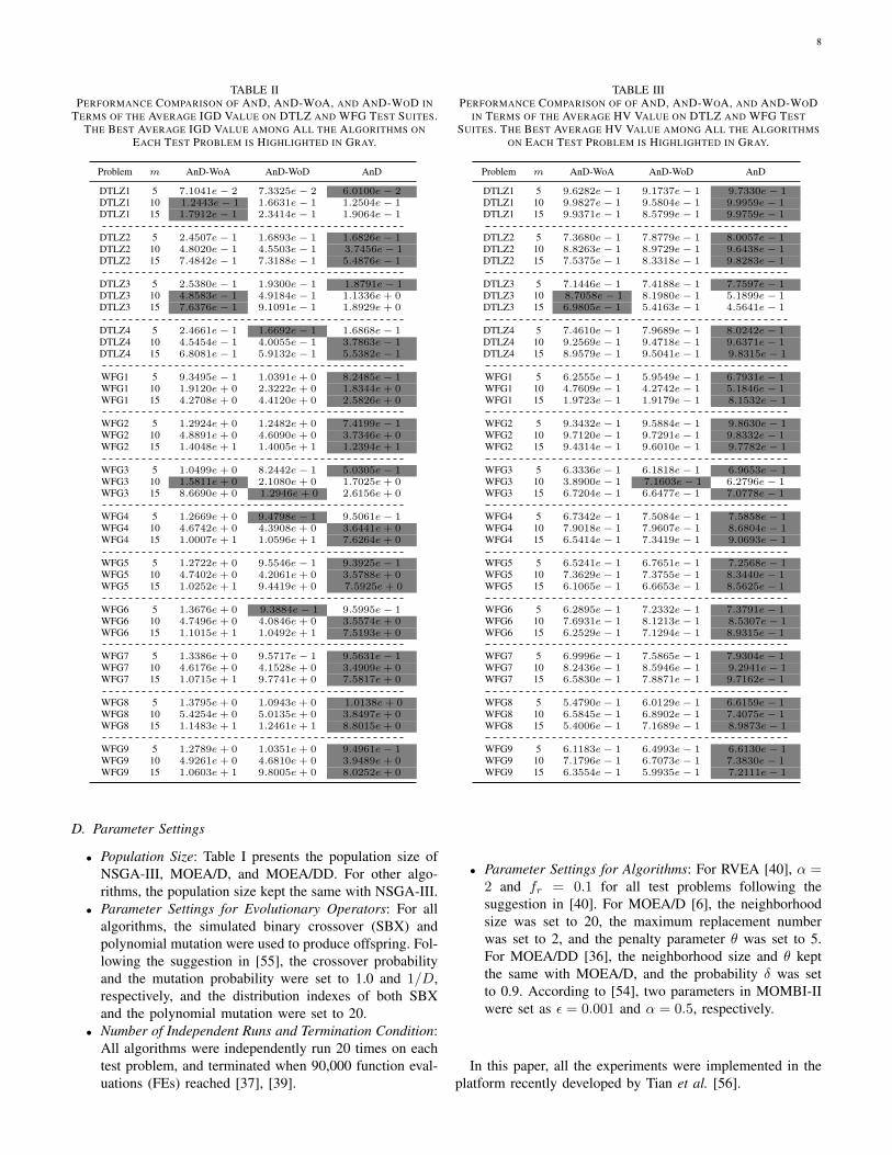
TABLE IIPERFORMANCE COMPARISON OF AND, AND-WOA, AND AND-WOD IN

TERMS OF THE AVERAGE IGD VALUE ON DTLZ AND WFG TEST SUITES.THE BEST AVERAGE IGD VALUE AMONG ALL THE ALGORITHMS ON

EACH TEST PROBLEM IS HIGHLIGHTED IN GRAY.

Problem m AnD-WoA AnD-WoD AnD

DTLZ1 5 7.1041e− 2 7.3325e− 2 6.0100e− 2DTLZ1 10 1.2443e− 1 1.6631e− 1 1.2504e− 1DTLZ1 15 1.7912e− 1 2.3414e− 1 1.9064e− 1

DTLZ2 5 2.4507e− 1 1.6893e− 1 1.6826e− 1DTLZ2 10 4.8020e− 1 4.5503e− 1 3.7456e− 1DTLZ2 15 7.4842e− 1 7.3188e− 1 5.4876e− 1

DTLZ3 5 2.5380e− 1 1.9300e− 1 1.8791e− 1DTLZ3 10 4.8583e− 1 4.9184e− 1 1.1336e+ 0DTLZ3 15 7.6376e− 1 9.1091e− 1 1.8929e+ 0

DTLZ4 5 2.4661e− 1 1.6692e− 1 1.6868e− 1DTLZ4 10 4.5454e− 1 4.0055e− 1 3.7863e− 1DTLZ4 15 6.8081e− 1 5.9132e− 1 5.5382e− 1

WFG1 5 9.3495e− 1 1.0391e+ 0 8.2485e− 1WFG1 10 1.9120e+ 0 2.3222e+ 0 1.8344e+ 0WFG1 15 4.2708e+ 0 4.4120e+ 0 2.5826e+ 0

WFG2 5 1.2924e+ 0 1.2482e+ 0 7.4199e− 1WFG2 10 4.8891e+ 0 4.6090e+ 0 3.7346e+ 0WFG2 15 1.4048e+ 1 1.4005e+ 1 1.2394e+ 1

WFG3 5 1.0499e+ 0 8.2442e− 1 5.0305e− 1WFG3 10 1.5811e+ 0 2.1080e+ 0 1.7025e+ 0WFG3 15 8.6690e+ 0 1.2946e+ 0 2.6156e+ 0

WFG4 5 1.2669e+ 0 9.4798e− 1 9.5061e− 1WFG4 10 4.6742e+ 0 4.3908e+ 0 3.6441e+ 0WFG4 15 1.0007e+ 1 1.0596e+ 1 7.6264e+ 0

WFG5 5 1.2722e+ 0 9.5546e− 1 9.3925e− 1WFG5 10 4.7402e+ 0 4.2061e+ 0 3.5788e+ 0WFG5 15 1.0252e+ 1 9.4419e+ 0 7.5925e+ 0

WFG6 5 1.3676e+ 0 9.3884e− 1 9.5995e− 1WFG6 10 4.7496e+ 0 4.0846e+ 0 3.5574e+ 0WFG6 15 1.1015e+ 1 1.0492e+ 1 7.5193e+ 0

WFG7 5 1.3386e+ 0 9.5717e− 1 9.5631e− 1WFG7 10 4.6176e+ 0 4.1528e+ 0 3.4909e+ 0WFG7 15 1.0715e+ 1 9.7741e+ 0 7.5817e+ 0

WFG8 5 1.3795e+ 0 1.0943e+ 0 1.0138e+ 0WFG8 10 5.4254e+ 0 5.0135e+ 0 3.8497e+ 0WFG8 15 1.1483e+ 1 1.2461e+ 1 8.8015e+ 0

WFG9 5 1.2789e+ 0 1.0351e+ 0 9.4961e− 1WFG9 10 4.9261e+ 0 4.6810e+ 0 3.9489e+ 0WFG9 15 1.0603e+ 1 9.8005e+ 0 8.0252e+ 0

D. Parameter Settings

• Population Size: Table I presents the population size ofNSGA-III, MOEA/D, and MOEA/DD. For other algo-rithms, the population size kept the same with NSGA-III.

• Parameter Settings for Evolutionary Operators: For allalgorithms, the simulated binary crossover (SBX) andpolynomial mutation were used to produce offspring. Fol-lowing the suggestion in [55], the crossover probabilityand the mutation probability were set to 1.0 and 1/D,respectively, and the distribution indexes of both SBXand the polynomial mutation were set to 20.

• Number of Independent Runs and Termination Condition:All algorithms were independently run 20 times on eachtest problem, and terminated when 90,000 function eval-uations (FEs) reached [37], [39].

TABLE IIIPERFORMANCE COMPARISON OF OF AND, AND-WOA, AND AND-WOD

IN TERMS OF THE AVERAGE HV VALUE ON DTLZ AND WFG TESTSUITES. THE BEST AVERAGE HV VALUE AMONG ALL THE ALGORITHMS

ON EACH TEST PROBLEM IS HIGHLIGHTED IN GRAY.

Problem m AnD-WoA AnD-WoD AnD

DTLZ1 5 9.6282e− 1 9.1737e− 1 9.7330e− 1DTLZ1 10 9.9827e− 1 9.5804e− 1 9.9959e− 1DTLZ1 15 9.9371e− 1 8.5799e− 1 9.9759e− 1

DTLZ2 5 7.3680e− 1 7.8779e− 1 8.0057e− 1DTLZ2 10 8.8263e− 1 8.9729e− 1 9.6438e− 1DTLZ2 15 7.5375e− 1 8.3318e− 1 9.8283e− 1

DTLZ3 5 7.1446e− 1 7.4188e− 1 7.7597e− 1DTLZ3 10 8.7058e− 1 8.1980e− 1 5.1899e− 1DTLZ3 15 6.9805e− 1 5.4163e− 1 4.5641e− 1

DTLZ4 5 7.4610e− 1 7.9689e− 1 8.0242e− 1DTLZ4 10 9.2569e− 1 9.4718e− 1 9.6371e− 1DTLZ4 15 8.9579e− 1 9.5041e− 1 9.8315e− 1

WFG1 5 6.2555e− 1 5.9549e− 1 6.7931e− 1WFG1 10 4.7609e− 1 4.2742e− 1 5.1846e− 1WFG1 15 1.9723e− 1 1.9179e− 1 8.1532e− 1

WFG2 5 9.3432e− 1 9.5884e− 1 9.8630e− 1WFG2 10 9.7120e− 1 9.7291e− 1 9.8332e− 1WFG2 15 9.4314e− 1 9.6010e− 1 9.7782e− 1

WFG3 5 6.3336e− 1 6.1818e− 1 6.9653e− 1WFG3 10 3.8900e− 1 7.1603e− 1 6.2796e− 1WFG3 15 6.7204e− 1 6.6477e− 1 7.0778e− 1

WFG4 5 6.7342e− 1 7.5084e− 1 7.5858e− 1WFG4 10 7.9018e− 1 7.9607e− 1 8.6804e− 1WFG4 15 6.5414e− 1 7.3419e− 1 9.0693e− 1

WFG5 5 6.5241e− 1 6.7651e− 1 7.2568e− 1WFG5 10 7.3629e− 1 7.3755e− 1 8.3440e− 1WFG5 15 6.1065e− 1 6.6653e− 1 8.5625e− 1

WFG6 5 6.2895e− 1 7.2332e− 1 7.3791e− 1WFG6 10 7.6931e− 1 8.1213e− 1 8.5307e− 1WFG6 15 6.2529e− 1 7.1294e− 1 8.9315e− 1

WFG7 5 6.9996e− 1 7.5865e− 1 7.9304e− 1WFG7 10 8.2436e− 1 8.5946e− 1 9.2941e− 1WFG7 15 6.5830e− 1 7.8871e− 1 9.7162e− 1

WFG8 5 5.4790e− 1 6.0129e− 1 6.6159e− 1WFG8 10 6.5845e− 1 6.8902e− 1 7.4075e− 1WFG8 15 5.4006e− 1 7.1689e− 1 8.9873e− 1

WFG9 5 6.1183e− 1 6.4993e− 1 6.6130e− 1WFG9 10 7.1796e− 1 6.7073e− 1 7.3830e− 1WFG9 15 6.3554e− 1 5.9935e− 1 7.2111e− 1

• Parameter Settings for Algorithms: For RVEA [40], α =2 and fr = 0.1 for all test problems following thesuggestion in [40]. For MOEA/D [6], the neighborhoodsize was set to 20, the maximum replacement numberwas set to 2, and the penalty parameter θ was set to 5.For MOEA/DD [36], the neighborhood size and θ keptthe same with MOEA/D, and the probability δ was setto 0.9. According to [54], two parameters in MOMBI-IIwere set as ε = 0.001 and α = 0.5, respectively.

In this paper, all the experiments were implemented in theplatform recently developed by Tian et al. [56].

9

TABLE IVPERFORMANCE COMPARISON BETWEEN AND AND SEVEN STATE-OF-THE-ART MAOEAS IN TERMS OF THE AVERAGE IGD VALUE ON DTLZ TEST

SUITE. THE BEST AND SECOND BEST AVERAGE IGD VALUES AMONG ALL THE ALGORITHMS ON EACH TEST PROBLEM ARE HIGHLIGHTED IN GRAYAND LIGHT GRAY, RESPECTIVELY.

Problem m RVEA SPEA2+SDE MOEA/D NSGA-III MOMBI-II MOEA/DD Two Arch2 AnD

DTLZ1 5 5.2408e− 2 5.0463e− 2 5.2640e− 2 5.2550e− 2 5.2675e− 2 5.2435e− 2 5.3565e− 2 6.0100e− 2DTLZ1 10 1.4004e− 1 1.1292e− 1 1.1831e− 1 1.8856e− 1 2.1156e− 1 1.2387e− 1 1.2356e− 1 1.2504e− 1DTLZ1 15 1.8157e− 1 1.6530e− 1 1.6486e− 1 2.6475e− 1 3.1515e− 1 1.6710e− 1 1.8887e− 1 1.9064e− 1

DTLZ2 5 1.6124e− 1 1.8868e− 1 1.6124e− 1 1.6125e− 1 1.6307e− 1 1.6124e− 1 1.7374e− 1 1.6826e− 1DTLZ2 10 4.1870e− 1 3.8855e− 1 4.2106e− 1 4.9906e− 1 4.1920e− 1 4.2108e− 1 4.5879e− 1 3.7456e− 1DTLZ2 15 5.7768e− 1 5.5854e− 1 5.7862e− 1 6.4743e− 1 8.3078e− 1 5.7824e− 1 6.7923e− 1 5.4876e− 1

DTLZ3 5 1.7390e− 1 1.8818e− 1 1.6662e− 1 1.7486e− 1 1.7057e− 1 1.6305e− 1 2.2382e− 1 1.8791e− 1DTLZ3 10 6.4615e− 1 3.9359e− 1 8.3022e− 1 9.5607e+ 0 4.8416e− 1 4.5511e− 1 1.8047e+ 0 1.1336e+ 0DTLZ3 15 7.3919e− 1 5.7993e− 1 1.1593e+ 0 3.1400e+ 1 1.1082e+ 0 5.9058e− 1 6.6586e+ 0 1.8929e+ 0

DTLZ4 5 1.6122e− 1 1.8854e− 1 4.6392e− 1 1.6128e− 1 1.6474e− 1 1.6122e− 1 1.7605e− 1 1.6868e− 1DTLZ4 10 4.1616e− 1 3.9027e− 1 6.2527e− 1 4.4139e− 1 4.2156e− 1 4.2107e− 1 4.5855e− 1 3.7863e− 1DTLZ4 15 5.8259e− 1 5.5802e− 1 7.7231e− 1 6.2785e− 1 5.9901e− 1 5.8698e− 1 6.7621e− 1 5.5382e− 1

TABLE VPERFORMANCE COMPARISON BETWEEN AND AND SEVEN STATE-OF-THE-ART MAOEAS IN TERMS OF THE AVERAGE HV VALUE ON DTLZ TEST

SUITE. THE BEST AND SECOND BEST AVERAGE HV VALUES AMONG ALL THE ALGORITHMS ON EACH TEST PROBLEM ARE HIGHLIGHTED IN GRAYAND LIGHT GRAY, RESPECTIVELY

Problem m RVEA SPEA2+SDE MOEA/D NSGA-III MOMBI-II MOEA/DD Two Arch2 AnD

DTLZ1 5 9.7971e− 1 9.6924e− 1 9.7942e− 1 9.7962e− 1 9.7942e− 1 9.7977e− 1 9.7582e− 1 9.7330e− 1DTLZ1 10 9.9868e− 1 9.9598e− 1 9.9826e− 1 9.1305e− 1 9.6719e− 1 9.9962e− 1 9.9507e− 1 9.9894e− 1DTLZ1 15 9.9950e− 1 9.9122e− 1 9.5880e− 1 9.0076e− 1 8.2655e− 1 9.9707e− 1 9.8287e− 1 9.9759e− 1

DTLZ2 5 8.1234e− 1 8.1125e− 1 8.1254e− 1 8.1233e− 1 8.1174e− 1 8.1247e− 1 7.6937e− 1 8.0057e− 1DTLZ2 10 9.7440e− 1 9.7222e− 1 9.7529e− 1 9.2862e− 1 9.7439e− 1 9.7531e− 1 7.7695e− 1 9.6438e− 1DTLZ2 15 9.8964e− 1 9.8403e− 1 9.8841e− 1 9.3018e− 1 8.4042e− 1 9.9015e− 1 6.3825e− 1 9.8283e− 1

DTLZ3 5 7.7880e− 1 8.0874e− 1 7.8499e− 1 7.7721e− 1 8.0386e− 1 7.9779e− 1 7.2701e− 1 7.7597e− 1DTLZ3 10 7.0475e− 1 9.6885e− 1 4.9755e− 1 0.0000e+ 0 9.3247e− 1 9.2789e− 1 1.6481e− 1 5.1899e− 1DTLZ3 15 7.6387e− 1 9.7532e− 1 2.3293e− 1 0.0000e+ 0 4.3883e− 1 9.7556e− 1 0.0000e+ 0 4.5641e− 1

DTLZ4 5 8.1251e− 1 8.1225e− 1 6.6181e− 1 8.1186e− 1 8.1128e− 1 8.1256e− 1 7.5774e− 1 8.0242e− 1DTLZ4 10 9.7383e− 1 9.7124e− 1 8.7615e− 1 9.6258e− 1 9.7453e− 1 9.7536e− 1 7.8132e− 1 9.6371e− 1DTLZ4 15 9.8789e− 1 9.8745e− 1 8.8487e− 1 9.5702e− 1 9.8474e− 1 9.8837e− 1 6.3605e− 1 9.8315e− 1

V. RESULTS AND DISCUSSIONS

A. Benefit of Two Strategies

Firstly, we are interested in identifying the benefit of twocrucial strategies of AnD: angel-based selection and shift-based density estimation. To this end, two variants of AnDwere devised named as AnD-WoA and AnD-WoD, respec-tively. In AnD-WoA, the angle-based selection was eliminated.Instead, the individuals in the union population Ut weresorted based on their shift-based density values [30] and Nindividuals with the highest density values were removedfrom Ut. In AnD-WoD, the shift-based density estimation wasabandoned. As an alternative, for two individuals with theminimum vector angle, their Euclidean distances to the idealpoint were computed and the one with the larger Euclideandistance was deleted [50], [47]. The comparative experimentsbetween AnD and its two variants were carried out on DTLZand WFG test suites. The IGD and HV values are shown inTables II and III, respectively.

From Tables II and III, it is evident that AnD outperformsits two variants on a vast majority of test problems. In termsof the IGD metric, AnD obtains the best performance on30 out of 39 test problems, while AnD-WoA and AnD-WoD achieve the best performance on only five and four

test problems, respectively. With respect to the HV metric,AnD performs the best on 36 test problems. Nevertheless,AnD-WoA and AnD-WoD perform the best on no more thantwo test problems. The reason for the above results seemsobvious. Compared with AnD, AnD-WoA discards the angle-based selection, therefore it is unable to maintain the diversityof search directions. Regarding AnD-WoD, it replaces theshift-based density estimation with the Euclidean distance.However, the Euclidean distance only considers an individual’sconvergence property; thus, it is less reasonable than the shift-based density estimation which takes both the diversity andconvergence into account.

From the above discussions, we can conclude that the angel-based selection and the shift-based density estimation are twoindispensable strategies in AnD.

B. Comparison with Seven State-of-the-Art MaOEAs

Subsequently, we compared the performance of AnD withthat of the seven peer algorithms introduced in Section IV-Con DTLZ and WFG test suites in terms of the IGD andHV metrics. The experimental results are summarized inTables IV–VII. At our first glance, RVEA, SPEA2+SDE, andMOEA/DD can achieve superior performance on DTLZ test

10

1 2 3 4 5 6 7 8 9 10

Objective NO.

0

0.1

0.2

0.3

0.4

0.5

0.6

Obj

ectiv

e V

alue

(a) RVEA

1 2 3 4 5 6 7 8 9 10

Objective NO.

0

0.1

0.2

0.3

0.4

0.5

0.6

Obj

ectiv

e V

alue

(b) SPEA2+SDE

1 2 3 4 5 6 7 8 9 10

Objective NO.

0

0.1

0.2

0.3

0.4

0.5

0.6

Obj

ectiv

e V

alue

(c) MOEA/D

1 2 3 4 5 6 7 8 9 10

Objective NO.

0

0.1

0.2

0.3

0.4

0.5

0.6

0.7

0.8

Obj

ectiv

e V

alue

(d) NSGA-III

1 2 3 4 5 6 7 8 9 10

Objective NO.

0

0.1

0.2

0.3

0.4

0.5

0.6

Obj

ectiv

e V

alue

(e) MOMBI-II

1 2 3 4 5 6 7 8 9 10

Objective NO.

0

0.1

0.2

0.3

0.4

0.5

0.6

Obj

ectiv

e V

alue

(f) MOEA/DD

1 2 3 4 5 6 7 8 9 10

Objective NO.

0

0.1

0.2

0.3

0.4

0.5

0.6

Obj

ectiv

e V

alue

(g) Two Arch2

1 2 3 4 5 6 7 8 9 10

Objective NO.

0

0.2

0.4

0.6

0.8

1

Obj

ectiv

e V

alue

(h) AnD

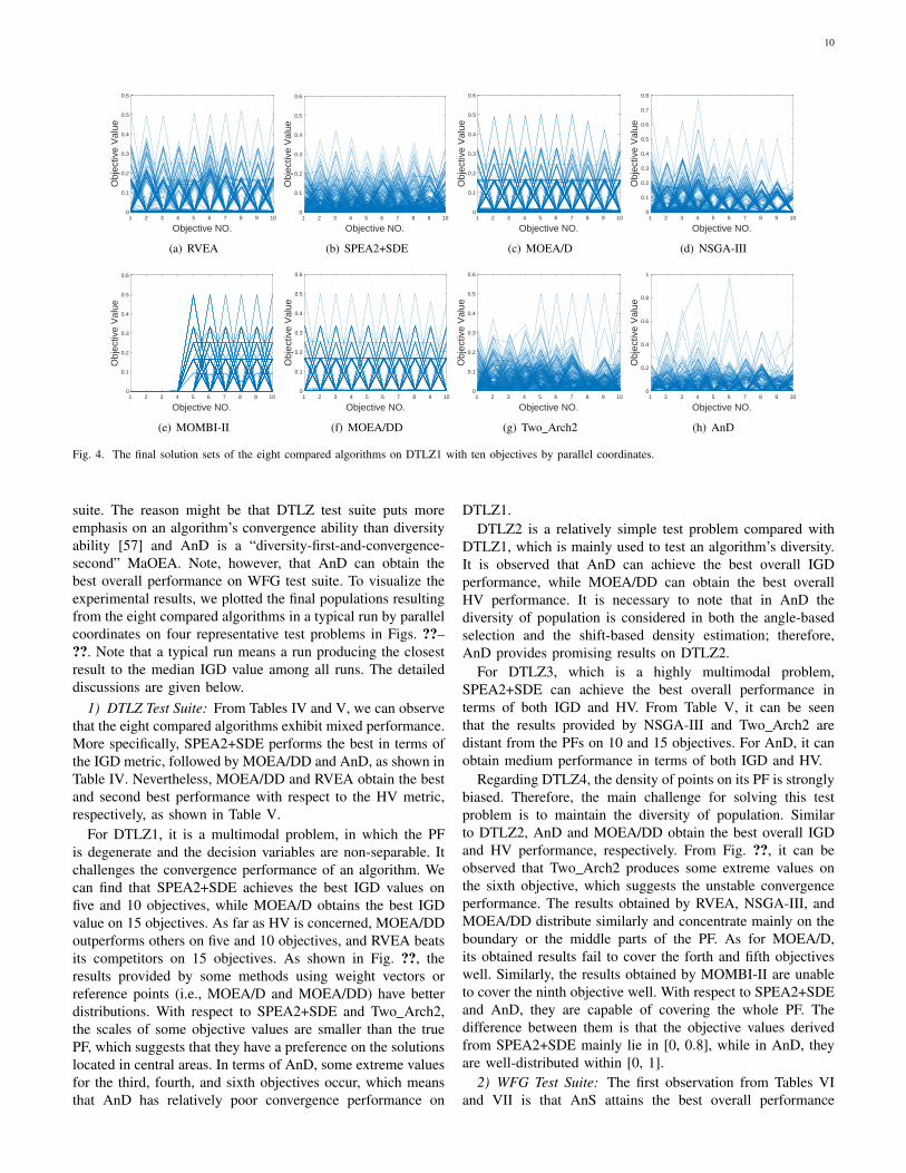
Fig. 4. The final solution sets of the eight compared algorithms on DTLZ1 with ten objectives by parallel coordinates.

suite. The reason might be that DTLZ test suite puts moreemphasis on an algorithm’s convergence ability than diversityability [57] and AnD is a “diversity-first-and-convergence-second” MaOEA. Note, however, that AnD can obtain thebest overall performance on WFG test suite. To visualize theexperimental results, we plotted the final populations resultingfrom the eight compared algorithms in a typical run by parallelcoordinates on four representative test problems in Figs. ??–??. Note that a typical run means a run producing the closestresult to the median IGD value among all runs. The detaileddiscussions are given below.

1) DTLZ Test Suite: From Tables IV and V, we can observethat the eight compared algorithms exhibit mixed performance.More specifically, SPEA2+SDE performs the best in terms ofthe IGD metric, followed by MOEA/DD and AnD, as shown inTable IV. Nevertheless, MOEA/DD and RVEA obtain the bestand second best performance with respect to the HV metric,respectively, as shown in Table V.

For DTLZ1, it is a multimodal problem, in which the PFis degenerate and the decision variables are non-separable. Itchallenges the convergence performance of an algorithm. Wecan find that SPEA2+SDE achieves the best IGD values onfive and 10 objectives, while MOEA/D obtains the best IGDvalue on 15 objectives. As far as HV is concerned, MOEA/DDoutperforms others on five and 10 objectives, and RVEA beatsits competitors on 15 objectives. As shown in Fig. ??, theresults provided by some methods using weight vectors orreference points (i.e., MOEA/D and MOEA/DD) have betterdistributions. With respect to SPEA2+SDE and Two Arch2,the scales of some objective values are smaller than the truePF, which suggests that they have a preference on the solutionslocated in central areas. In terms of AnD, some extreme valuesfor the third, fourth, and sixth objectives occur, which meansthat AnD has relatively poor convergence performance on

DTLZ1.DTLZ2 is a relatively simple test problem compared with

DTLZ1, which is mainly used to test an algorithm’s diversity.It is observed that AnD can achieve the best overall IGDperformance, while MOEA/DD can obtain the best overallHV performance. It is necessary to note that in AnD thediversity of population is considered in both the angle-basedselection and the shift-based density estimation; therefore,AnD provides promising results on DTLZ2.

For DTLZ3, which is a highly multimodal problem,SPEA2+SDE can achieve the best overall performance interms of both IGD and HV. From Table V, it can be seenthat the results provided by NSGA-III and Two Arch2 aredistant from the PFs on 10 and 15 objectives. For AnD, it canobtain medium performance in terms of both IGD and HV.

Regarding DTLZ4, the density of points on its PF is stronglybiased. Therefore, the main challenge for solving this testproblem is to maintain the diversity of population. Similarto DTLZ2, AnD and MOEA/DD obtain the best overall IGDand HV performance, respectively. From Fig. ??, it can beobserved that Two Arch2 produces some extreme values onthe sixth objective, which suggests the unstable convergenceperformance. The results obtained by RVEA, NSGA-III, andMOEA/DD distribute similarly and concentrate mainly on theboundary or the middle parts of the PF. As for MOEA/D,its obtained results fail to cover the forth and fifth objectiveswell. Similarly, the results obtained by MOMBI-II are unableto cover the ninth objective well. With respect to SPEA2+SDEand AnD, they are capable of covering the whole PF. Thedifference between them is that the objective values derivedfrom SPEA2+SDE mainly lie in [0, 0.8], while in AnD, theyare well-distributed within [0, 1].

2) WFG Test Suite: The first observation from Tables VIand VII is that AnS attains the best overall performance

11

1 2 3 4 5 6 7 8 9 10

Objective NO.

0

0.2

0.4

0.6

0.8

1

1.2

Obj

ectiv

e V

alue

(a) RVEA

1 2 3 4 5 6 7 8 9 10

Objective NO.

0

0.2

0.4

0.6

0.8

1

1.2

Obj

ectiv

e V

alue

(b) SPEA2+SDE

1 2 3 4 5 6 7 8 9 10

Objective NO.

0

0.2

0.4

0.6

0.8

1

1.2

Obj

ectiv

e V

alue

(c) MOEA/D

1 2 3 4 5 6 7 8 9 10

Objective NO.

0

0.2

0.4

0.6

0.8

1

1.2

Obj

ectiv

e V

alue

(d) NSGA-III

1 2 3 4 5 6 7 8 9 10

Objective NO.

0

0.2

0.4

0.6

0.8

1

1.2

Obj

ectiv

e V

alue

(e) MOMBI-II

1 2 3 4 5 6 7 8 9 10

Objective NO.

0

0.2

0.4

0.6

0.8

1

1.2

Obj

ectiv

e V

alue

(f) MOEA/DD

1 2 3 4 5 6 7 8 9 10

Objective NO.

0

0.5

1

1.5

Obj

ectiv

e V

alue

(g) Two Arch2

1 2 3 4 5 6 7 8 9 10

Objective NO.

0

0.2

0.4

0.6

0.8

1

1.2

Obj

ectiv

e V

alue

(h) AnD

Fig. 5. The final solution sets of the eight compared algorithms on DTLZ4 with ten objectives by parallel coordinates.

TABLE VIPERFORMANCE COMPARISON BETWEEN AND AND SEVEN STATE-OF-THE-ART MAOEAS IN TERMS OF THE AVERAGE IGD VALUE ON WFG TEST

SUITE. THE BEST AND SECOND BEST AVERAGE IGD VALUES AMONG ALL THE ALGORITHMS ON EACH TEST PROBLEM ARE HIGHLIGHTED IN GRAYAND LIGHT GRAY, RESPECTIVELY.

Problem m RVEA SPEA2+SDE MOEA/D NSGA-III MOMBI-II MOEA/DD Two Arch2 AnS

WFG1 5 1.2380e+ 0 4.5051e− 1 1.4719e+ 0 1.3003e+ 0 7.3247e− 1 1.7863e+ 0 9.5226e− 1 8.2485e− 1WFG1 10 2.4159e+ 0 1.5483e+ 0 3.5093e+ 0 2.3319e+ 0 2.9849e+ 0 2.7158e+ 0 2.2678e+ 0 1.8344e+ 0WFG1 15 3.4128e+ 0 3.0000e+ 0 5.4507e+ 0 3.6069e+ 0 6.0947e+ 0 4.2376e+ 0 3.1632e+ 0 2.5826e+ 0

WFG2 5 7.3061e− 1 9.9429e− 1 2.9028e+ 0 6.2450e− 1 1.2746e+ 0 1.9358e+ 0 4.7796e− 1 7.4199e− 1WFG2 10 3.6478e+ 0 5.4046e+ 0 1.1021e+ 1 4.0066e+ 0 3.9907e+ 0 1.1009e+ 1 1.9916e+ 0 3.7346e+ 0WFG2 15 1.2716e+ 1 1.4549e+ 1 1.6855e+ 1 1.2405e+ 1 1.9653e+ 1 1.5737e+ 1 5.7470e+ 0 1.2394e+ 1

WFG3 5 6.4564e− 1 5.8114e− 1 1.0504e+ 0 4.7212e− 1 9.5483e− 1 6.5805e− 1 3.6891e− 1 5.0305e− 1WFG3 10 3.0551e+ 0 1.7028e+ 0 8.6850e+ 0 8.7259e− 1 9.3633e+ 0 2.8279e+ 0 1.2887e+ 0 1.7025e+ 0WFG3 15 6.2924e+ 0 4.5129e+ 0 1.6375e+ 1 3.2111e+ 0 1.6002e+ 1 1.4214e+ 1 2.5444e+ 0 2.6156e+ 0

WFG4 5 9.4475e− 1 1.1148e+ 0 1.6793e+ 0 9.5187e− 1 1.7483e+ 0 1.0314e+ 0 9.7618e− 1 9.5061e− 1WFG4 10 3.8034e+ 0 4.1323e+ 0 8.9303e+ 0 4.0807e+ 0 8.3168e+ 0 5.2137e+ 0 4.5821e+ 0 3.6441e+ 0WFG4 15 8.7523e+ 0 8.2858e+ 0 1.6011e+ 1 8.9661e+ 0 2.3009e+ 1 9.1948e+ 0 9.7013e+ 0 7.6264e+ 0

WFG5 5 9.3668e− 1 1.1233e+ 0 1.5112e+ 0 9.3688e− 1 1.6929e+ 0 1.0146e+ 0 9.7161e− 1 9.3925e− 1WFG5 10 3.8534e+ 0 4.0242e+ 0 8.6325e+ 0 3.8863e+ 0 7.2474e+ 0 5.9057e+ 0 4.5803e+ 0 3.5788e+ 0WFG5 15 8.2300e+ 0 1.0363e+ 1 1.6180e+ 1 8.6808e+ 0 2.7050e+ 1 1.3822e+ 1 9.6726e+ 0 7.5925e+ 0

WFG6 5 9.4927e− 1 1.1683e+ 04 1.9082e+ 0 9.5167e− 1 1.6161e+ 0 1.0294e+ 0 9.8289e− 1 9.5995e− 1WFG6 10 3.8553e+ 0 4.1209e+ 0 9.7139e+ 0 3.9288e+ 0 7.5219e+ 0 5.4913e+ 0 4.5845e+ 0 3.5574e+ 0WFG6 15 8.5768e+ 0 9.3893e+ 0 1.6228e+ 1 9.0585e+ 0 2.3092e+ 1 1.3704e+ 1 9.7084e+ 0 7.5193e+ 0

WFG7 5 9.5376e− 1 1.1481e+ 0 1.7551e+ 0 9.5434e− 1 1.4084e+ 0 1.0384e+ 0 9.5596e− 1 9.5631e− 1WFG7 10 3.8105e+ 0 3.9180e+ 0 9.6364e+ 0 4.1474e+ 0 7.0575e+ 0 4.8005e+ 0 4.5546e+ 0 3.4909e+ 0WFG7 15 8.4477e+ 0 8.1509e+ 0 1.6400e+ 1 9.2815e+ 0 2.2087e+ 1 8.0829e+ 0 9.9669e+ 0 7.5817e+ 0

WFG8 5 9.8533e− 1 1.1560e+ 0 1.2965e+ 0 1.0084e+ 0 2.3995e+ 0 1.0543e+ 0 1.1102e+ 0 1.0138e+ 0WFG8 10 3.9040e+ 0 4.3343e+ 0 8.1439e+ 0 5.1141e+ 0 8.8767e+ 0 4.1808e+ 0 5.4467e+ 0 3.8497e+ 0WFG8 15 9.5526e+ 0 8.5588e+ 0 1.2660e+ 1 1.0520e+ 1 2.3945e+ 1 9.0171e+ 0 1.0866e+ 1 8.8015e+ 0

WFG9 5 9.1032e− 1 1.0663e+ 0 1.3802e+ 0 9.2301e− 1 2.2015e+ 0 1.0173e+ 0 1.0066e+ 0 9.4961e− 1WFG9 10 4.1319e+ 0 4.2572e+ 0 9.0024e+ 0 4.1250e+ 0 6.7789e+ 0 6.0132e+ 0 5.1443e+ 0 3.9489e+ 0WFG9 15 8.2901e+ 0 9.1482e+ 0 1.5257e+ 1 8.6989e+ 0 2.7200e+ 1 1.2606e+ 1 1.0647e+ 1 8.0252e+ 0

in terms of both IGD and HV. Next, we give the detaileddiscussions.

Table VI shows the IGD values resulting from the eightcompared algorithms. Clearly, AnS and RVEA are the two top

algorithms and they have a clear advantage over the other sixalgorithms on the majority of test problems. Actually, AnSprovides the best and second best IGD values on 12 andsix out of 27 test problems, respectively. As for RVEA, it

12

TABLE VIIPERFORMANCE COMPARISON BETWEEN AND AND SEVEN STATE-OF-THE-ART MAOEAS IN TERMS OF THE AVERAGE HV VALUE ON WFG TEST

SUITE. THE BEST AND SECOND BEST AVERAGE HV VALUES AMONG ALL THE ALGORITHMS ON EACH TEST PROBLEM ARE HIGHLIGHTED IN GRAYAND LIGHT GRAY, RESPECTIVELY.

Problem m RVEA SPEA2+SDE MOEA/D NSGA-III MOMBI-II MOEA/DD Two Arch2 AnS

WFG1 5 5.2614e− 1 8.5804e− 1 6.9318e− 1 5.0964e− 1 9.8249e− 1 3.7722e− 1 6.3042e− 1 6.7931e− 1WFG1 10 3.3523e− 1 6.1873e− 1 4.5187e− 1 4.2400e− 1 9.9177e− 1 2.8866e− 1 3.9733e− 1 5.1846e− 1WFG1 15 6.4838e− 1 6.4360e− 1 2.5320e− 1 5.6188e− 1 8.3535e− 1 8.5739e− 1 4.8177e− 1 8.1532e− 1

WFG2 5 9.5415e− 1 9.4272e− 1 7.4322e− 1 9.6190e− 1 9.7075e− 1 9.2248e− 1 9.7553e− 1 9.8630e− 1WFG2 10 9.0610e− 1 9.5588e− 1 7.3343e− 1 9.4637e− 1 7.5468e− 1 8.8639e− 1 9.4264e− 1 9.8332e− 1WFG2 15 7.6722e− 1 9.3104e− 1 6.7549e− 1 9.1018e− 1 5.4736e− 1 8.0398e− 1 9.7373e− 1 9.7782e− 1

WFG3 5 2.5974e− 2 6.7116e− 1 5.9385e− 1 7.1066e− 1 6.7204e− 1 6.6812e− 1 7.2408e− 1 6.9653e− 1WFG3 10 3.7874e− 1 5.6384e− 1 2.2239e− 1 6.0532e− 1 2.7517e− 1 2.5414e− 1 7.3015e− 1 6.2796e− 1WFG3 15 4.6421e− 1 6.9188e− 1 3.6466e− 1 7.3573e− 1 3.2567e− 1 6.5152e− 1 7.5401e− 1 7.0778e− 1

WFG4 5 7.4868e− 1 7.5476e− 1 6.4367e− 1 7.4082e− 1 6.6036e− 1 7.3706e− 1 7.1734e− 1 7.5858e− 1WFG4 10 8.3259e− 1 8.2460e− 1 3.7213e− 1 8.6530e− 1 6.2085e− 1 7.8810e− 1 6.7389e− 1 8.6804e− 1WFG4 15 7.6663e− 1 8.7028e− 1 1.6598e− 1 7.8689e− 1 3.3596e− 1 8.6369e− 1 6.1921e− 1 9.0693e− 1

WFG5 5 7.3031e− 1 7.1458e− 1 6.4534e− 1 7.2793e− 1 6.1046e− 1 7.0839e− 1 6.8516e− 1 7.2568e− 1WFG5 10 8.4286e− 1 7.9010e− 1 3.7997e− 1 8.4800e− 1 5.5075e− 1 6.8552e− 1 6.1423e− 1 8.3440e− 1WFG5 15 8.4490e− 1 7.7143e− 1 1.1919e− 1 7.8855e− 1 2.1399e− 1 3.9362e− 1 5.1556e− 1 8.5625e− 1

WFG6 5 7.3194e− 1 7.3388e− 1 5.4052e− 1 7.2387e− 1 6.5647e− 1 7.1624e− 1 6.8634e− 1 7.3791e− 1WFG6 10 8.6056e− 1 8.2632e− 1 1.9400e− 1 8.5875e− 1 6.2132e− 1 7.5777e− 1 6.0675e− 1 8.5307e− 1WFG6 15 8.6801e− 1 8.4484e− 1 9.4497e− 2 8.5336e− 1 3.3801e− 1 4.4625e− 1 5.1359e− 1 8.9315e− 1

WFG7 5 7.8637e− 1 7.8067e− 1 6.3867e− 1 7.7461e− 1 7.6659e− 1 7.6365e− 1 7.5484e− 1 7.9304e− 1WFG7 10 8.8809e− 1 8.9075e− 1 2.3503e− 1 9.1733e− 1 7.4944e− 1 8.5089e− 1 6.6219e− 1 9.2941e− 1WFG7 15 7.2147e− 1 9.2918e− 1 1.2338e− 1 8.3698e− 1 4.2995e− 1 9.1768e− 1 6.0513e− 1 9.7162e− 1

WFG8 5 6.4019e− 1 6.7275e− 1 5.0839e− 1 6.5130e− 1 3.5919e− 1 6.3295e− 1 6.1111e− 1 6.6159e− 1WFG8 10 6.0051e− 1 8.0185e− 1 7.3417e− 2 7.8469e− 1 4.6721e− 1 7.0977e− 1 4.4208e− 1 7.4075e− 1WFG8 15 3.8537e− 1 8.7264e− 1 3.4644e− 1 7.3358e− 1 2.9260e− 1 8.6234e− 1 3.5437e− 1 8.9873e− 1

WFG9 5 6.8336e− 1 6.7929e− 1 5.8874e− 1 6.4825e− 1 3.8392e− 1 6.3831e− 1 6.3829e− 1 6.6130e− 1WFG9 10 7.0854e− 1 7.4727e− 1 1.5646e− 1 7.3520e− 1 5.1312e− 1 5.2354e− 1 5.6358e− 1 7.3830e− 1WFG9 15 6.1502e− 1 7.1075e− 1 6.0542e− 2 7.1895e− 1 2.0338e− 1 2.4844e− 1 4.4957e− 1 7.2111e− 1

1 2 3 4 5 6 7 8 9 10

Objective NO.

0

5

10

15

20

25

Obj

ectiv

e V

alue

(a) RVEA

1 2 3 4 5 6 7 8 9 10

Objective NO.

0

5

10

15

20

25

Obj

ectiv

e V

alue

(b) SPEA2+SDE

1 2 3 4 5 6 7 8 9 10

Objective NO.

0

1

2

3

4

5

6

Obj

ectiv

e V

alue

(c) MOEA/D

1 2 3 4 5 6 7 8 9 10

Objective NO.

0

5

10

15

20

25

Obj

ectiv

e V

alue

(d) NSGA-III

1 2 3 4 5 6 7 8 9 10

Objective NO.

0

5

10

15

20

25

Obj

ectiv

e V

alue

(e) MOMBI-II

1 2 3 4 5 6 7 8 9 10

Objective NO.

0

5

10

15

20

25

Obj

ectiv

e V

alue

(f) MOEA/DD

1 2 3 4 5 6 7 8 9 10

Objective NO.

0

5

10

15

20

25

Obj

ectiv

e V

alue

(g) Two Arch2

1 2 3 4 5 6 7 8 9 10

Objective NO.

0

5

10

15

20

25

Obj

ectiv

e V

alue

(h) AnD

Fig. 6. The final solution sets of the eight compared algorithms on WFG4 with ten objectives by parallel coordinates.

generates six best results and nine second best results. In ad-dition, SPEA2+SDE obtains three best results and two secondbest results, Two Arch2 produces five best results, NSGA-III shows one best result and seven second best results, and

MOEA/DD and MOMBI-II reach one second best result. Oneinteresting phenomenon we have observed is that the methodsbased on weight vectors or reference points (i.e., MOEA/D,MOEA/DD, NSGA-III, and MOMBI-II) seem to lose their

13

1 2 3 4 5 6 7 8 9 10

Objective NO.

0

5

10

15

20

25

Obj

ectiv

e V

alue

(a) RVEA

1 2 3 4 5 6 7 8 9 10

Objective NO.

0

5

10

15

20

25

Obj

ectiv

e V

alue

(b) SPEA2+SDE

1 2 3 4 5 6 7 8 9 10

Objective NO.

0

0.5

1

1.5

2

2.5

3

3.5

Obj

ectiv

e V

alue

(c) MOEA/D

1 2 3 4 5 6 7 8 9 10

Objective NO.

0

5

10

15

20

25

Obj

ectiv

e V

alue

(d) NSGA-III

1 2 3 4 5 6 7 8 9 10

Objective NO.

0

5

10

15

20

25

Obj

ectiv

e V

alue

(e) MOMBI-II

1 2 3 4 5 6 7 8 9 10

Objective NO.

0

5

10

15

20

25

Obj

ectiv

e V

alue

(f) MOEA/DD

1 2 3 4 5 6 7 8 9 10

Objective NO.

0

5

10

15

20

25

Obj

ectiv

e V

alue

(g) Two Arch2

1 2 3 4 5 6 7 8 9 10

Objective NO.

0

5

10

15

20

25

Obj

ectiv

e V

alue

(h) AnD

Fig. 7. The final solution sets of the eight compared algorithms on WFG7 with ten objectives by parallel coordinates.

0

5

10

15

20

25

30

35

better

similar

worse

Nu

mb

er o

f T

est

Pro

ble

ms

(a) IGD

0

5

10

15

20

25

30

35

40

better

similar

worse

Num

ber

of

Tes

t P

roble

ms

(b) HV

Fig. 8. Wilcoxon rank sum test between AnD and its seven competitors (i.e., RVEA, SPEA2+SDE, MOEA/D, NSGA-III, MOMBI-II, MOEA/DD, andTwo Arch2) on all the test problems (including DTLZ and WFG test suites) in terms of IGD and HV. “better“, “similar“ and “worse“ mean that a competitorperforms better than, similar to, and worse than AnD, respectively.

3.0235

3.7051

6.6026

4.0256

6.5769

4.6923 4.6923

2.7308

0

1

2

3

4

5

6

7

Av

erag

e R

ank

ing

o

f t

he

Fri

edm

an T

est

(a) IGD

3.5897 3.2692

6.6154

4.0897

5.5897

4.2436

5.7179

2.8846

0

1

2

3

4

5

6

7

Av

erag

e R

ank

ing

o

f t

he

Fri

edm

an T

est

(b) HV

Fig. 9. Friedman test on AnD and its seven competitors (i.e., RVEA, SPEA2+SDE, MOEA/D, NSGA-III, MOMBI-II, MOEA/DD, and Two Arch2) on allthe test problems (including DTLZ and WFG test suites) in terms of IGD and HV. The smaller the ranking, the better the performance of an algorithm.

effectiveness on this test suite. This can be attributed to thefact that the PFs of WFG test suite are irregular, discontinued

or mixed, and scaled with different ranges in each objective.Therefore, a well-distributed weight vectors/reference points

14

can not guarantee a good distribution of obtained solutions.Note, however, that RVEA, which also uses the referencevectors to guide the search, performs better than MOEA/D,MOEA/DD, NSGA-III, and MOMBI-II. It is perhaps becausethe usage of angle information helps RVEA to alleviate thisissue to some extent.

The HV values are given in Table VII. From Table VII,AnS and SPEA2+SDE achieve the best and second bestoverall performance, respectively. Specifically, AnS produces14 best results and three second best results out of 27 testproblems, and SPEA2+SDE shows three best results and eightsecond best results. It is also observed that AnS reachesthe best performance on WFG2, WFG4, WFG6, and WFG7.For MOMBI-II, Two Arch2, RVEA, and SPEA2+SDE, theyexhibit the best overall performance on WFG1, WFG3, WFG5,and WFG8, respectively. With regard to WFG9, AnS andSPEA2+SDE are the two best algorithms for solving it.

With the aim of revealing more details of the eight com-pared algorithms, their experimental results on both WFG4and WFG7 with ten objectives are presented by parallelcoordinates in Figs. 6 and 7, respectively. From Fig. 6,one can see that MOEA/D and MOEA/DD have relativelypoor distributions. It might be because they are lack of anormalization procedure before the evaluation of an individual.As for RVEA and MOMBI-II, the former fails to cover theseventh objective well, while the latter is unable to cover thefirst four objectives well. In terms of SPEA2+SDE, NSGA-III,Two Arch2, and AnD, all of them can cover the whole PF.The difference between them is that the results derived fromSPEA2+SDE, NSGA-III, and Two Arch2 concentrate mainlyon the boundary or the middle parts of the PF, while in AnD,the obtained results can spread out on the whole PF very well.The similar phenomena can also be observed in Fig. 7. AnDstill has the best distribution. Note that NSGA-III fails to coverthe first objective well.

3) Discussion: To analyze the overall performance on bothDTLZ and WFG test suites, the Wilcoxon rank sum test wasimplemented between AnD and the other seven MaOEAsin terms of both IGD and HV metrics. The statistical testresults are presented in Fig. 8. Fig. 8(a) gives the comparisonresults in terms of IGD. From Fig. 8(a), we can find thatAnD outperforms RVEA, SPEA2+SDE, MOEA/D, NSGA-III, MOMBI-II, MOEA/DD, and Two Arch2 on 21, 29, 31,23, 31, 29, and 29 test problems, respectively, while it loseson 10, eight, five, nine, six, eight, and seven test prob-lems, accordingly. The comparison results for HV is shownin Fig. 8(b). As shown in Fig. 8(b), AnD performs betterthan RAVE, SPEA2+SDE, MOEA/D, NSGA-III, MOMBI-II,MOEA/DD, and Two Arch2 on 22, 17, 31, 19, 26, 24, and 35test problems, respectively, while performs worse on 14, 14,five, eight, 11, 12, and four test problems, accordingly. Thus,we can conclude that AnD is able to obtain the better overallperformance compared with the seven competitors in terms ofboth IGD and HV.

Further, the Friedman test was also implemented on all thetest problems in terms of both IGD and HV. In the Friedmantest, the smaller the ranking, the better the performance of analgorithm. From Fig. 9, it is evident that AnD has the smallest

TABLE VIIIEXPERIMENTAL RESULTS (MEAN AND STANDARD DEVIATION) OF THEIGD AND HV VALUES ON C1-DTLZ1, C2-DTLZ2, AND C3-DTLZ4.THE BETTER RESULT BETWEEN C-AND AND C-NSGA-III ON EACH

TEST PROBLEM IS HIGHLIGHTED IN GRAY.

IGD m C-NSGA-III C-AnD

C1-DTLZ1 5 5.8093e− 2 (5.60e− 3) 5.4026e− 2 (5.46e− 3)C1-DTLZ1 10 1.2436e− 1 (4.98e− 3) 1.1237e− 1 (3.26e− 3)C1-DTLZ1 15 2.0774e− 1 (1.13e− 2) 1.7216e− 1 (2.01e− 3)

C2-DTLZ2 5 1.8916e− 1 (7.44e− 2) 1.5010e− 1 (6.73e− 3)C2-DTLZ2 10 3.7888e− 1 (1.20e− 1) 2.6826e− 1 (5.60e− 2)C2-DTLZ2 15 7.2215e− 1 (1.56e− 1) 2.6633e− 1 (1.62e− 1)

C3-DTLZ4 5 2.8139e− 1 (2.04e− 2) 2.8605e− 1 (1.40e− 2)C3-DTLZ4 10 5.7678e− 1 (6.60e− 2) 5.4039e− 1 (1.34e− 2)C3-DTLZ4 15 1.1089e+ 0 (2.72e− 1) 7.3981e− 1 (2.88e− 3)

HV m C-NSGA-III C-AnD

C1-DTLZ1 5 9.7255e− 1 (2.73e− 3) 9.7770e− 1 (1.90e− 3)C1-DTLZ1 10 9.8800e− 1 (1.05e− 2) 9.8803e− 1 (1.66e− 2)C1-DTLZ1 15 9.5938e− 1 (3.76e− 2) 9.9054e− 1 (1.19e− 2)

C2-DTLZ2 5 7.3902e− 1 (4.53e− 2) 7.4493e− 1 (3.45e− 3)C2-DTLZ2 10 8.3045e− 1 (7.04e− 2) 8.7759e− 1 (1.46e− 2)C2-DTLZ2 15 5.9223e− 1 (2.35e− 1) 9.0674e− 1 (1.65e− 1)

C3-DTLZ4 5 9.4462e− 1 (2.68e− 2) 9.5475e− 1 (1.61e− 3)C3-DTLZ4 10 9.9877e− 1 (2.51e− 3) 9.9909e− 1 (1.08e− 4)C3-DTLZ4 15 9.5658e− 1 (3.70e− 2) 9.9991e− 1 (1.84e− 5)

ranking in terms of both IGD and HV, followed by RVEA andSPEA2+SDE. For RVEA, it ranks the third best and the secondbest in terms of IGD and HV, respectively. For SPEA2+SDE,it works the second best and the third best in terms ofIGD and HV, respectively. The above results indicate that thealgorithm with either the shift-based density estimation (i.e.,SPEA2+SDE) or angle information (i.e., RVEA) is suitablefor solving MaOPs. Moreover, the algorithm with these twoelements (i.e., AnD) achieves the best performance, whichverifies the main motivation of this paper.

C. Constrained MaOPs

One may be interested in whether AnD can be applied tosolve constrained MaOPs, which are frequently encounteredin the real-world applications. To answer this question, AnDwas extended to cope with this kind of optimization problemand the resultant algorithm is called C-AnD.

The constraint-handling technique of C-AnD is inspired bythe feasibility rule [58], which is a well-known constraint-handling technique for constrained single-objective optimiza-tion problems. Firstly, we compute the degree of constraintviolation for each individual:

CV (x) =

J∑j=1

max0, gj(x)+

K∑k=1

|hk(x)| (8)

where gj ≥ 0 and hj = 0 denote the jth inequality constraintand the jth equality constraint, respectively, and J and K arethe number of inequality constraints and equality constraint,respectively. Subsequently, the number of feasible solutions inthe union population Ut is calculated. If the number of feasiblesolutions is larger than N , then Algorithm 2 is triggered to

15

select N feasible solutions from all the feasible solutions intothe next generation. Otherwise, we sort the individuals in Utaccording to their degree of constraint violations, and thenpick out N individuals with the smallest degree of constraintviolations into the next generation.

Overall, the implementation of C-AnD is simple. The per-formance of C-AnD was compared with C-NSGA-III [59],which is the constrained version of NSGA-III, on three repre-sentative constrained MaOPs, namely C1-DTLZ1, C2-DTLZ2,and C3-DTLZ4 with five, 10, and 15 objectives. Both C-AnDand C-NSGA-III were run 20 times independently for eachtest problem. In each run, the maximum number of FEs wasset to 180,000 for C1-DTLZ1, and 90,000 for C2-DTLZ2and C3-DTLZ4. The experimental results are summarized inTable VIII.

From Table VIII, it can be seen that C-AnD beats C-NSGA-III on all the test problems except C3-DTLZ4 withfive objectives in terms of IGD. Therefore, C-AnD is also asimple and effective algorithm for constrained many-objectiveoptimization. It is worth noting that there are no referencepoints in C-AnD, thus C-AnD does not experience the degen-eration of reference points as in constrained decomposition-based approaches.

VI. CONCLUSION

In this paper, a novel algorithm for dealing with MaOPs,named AnD, was proposed. AnD not only has a simplestructure, but also is free from the usage of the Pareto-dominance relation, weight vectors or reference points, andindicators. The main characteristic of AnD is making use oftwo strategies (i.e., the angle-based selection and the shift-based density estimation) to delete the poor individuals oneby one in the environmental selection.

The aim of the angle-based selection is to maintain thediversity of the search directions. It identifies a pair of in-dividuals with the minimum vector angle, which means thatthese two individuals search in the most similar direction.Subsequently, the shift-based density estimation is conductedto differentiate them by considering both the diversity andconvergence, and to remove the inferior one. We validatedthat these two strategies play very important roles and areindispensable in AnD. In addition, we compared AnD withseven state-of-the-art MaOEAs for solving MaOPs with upto 15 objective in DTLZ and WFG test suites. The experi-mental results indicated that, overall, AnD achieves the bestperformance in terms of both IGD and HV. Due to the factthat MaOPs in real world often include constraints, AnDwas further extended to solve constrained MaOPs and theexperimental results verified its effectiveness.

In the future, we will apply AnD to solve some MaOPsin the fields of engineering such as automotive lightweightdesign and adaptive walking of humanoid robots. Anotherpromising research direction is to combine AnD with otherkinds of MaOEAs such as Pareto-based, decomposition-basedand indicator-based approaches.

REFERENCES

[1] A. Zhou, B.-Y. Qu, H. Li, S.-Z. Zhao, P. N. Suganthan, and Q. Zhang,“Multiobjective evolutionary algorithms: A survey of the state of theart,” Swarm and Evolutionary Computation, vol. 1, no. 1, pp. 32–49,2011.

[2] H. Ishibuchi, N. Akedo, H. Ohyanagi, and Y. Nojima, “Behavior of EMOalgorithms on many-objective optimization problems with correlatedobjectives,” in 2011 IEEE Congress on Evolutionary Computation (CEC2011). IEEE, 2011, pp. 1465–1472.

[3] H. Ishibuchi, N. Akedo, and Y. Nojima, “Behavior of multiobjectiveevolutionary algorithms on many-objective knapsack problems,” IEEETransactions on Evolutionary Computation, vol. 19, no. 2, pp. 264–283,2015.

[4] K. Deb, A. Pratap, S. Agarwal, and T. Meyarivan, “A fast and elitistmultiobjective genetic algorithm: NSGA-II,” IEEE Transactions onEvolutionary Computation, vol. 6, no. 2, pp. 182–197, 2002.

[5] E. Zitzler, M. Laumanns, and L. Thiele, “SPEA2: Improving thestrength pareto evolutionary algorithm for multiobjective optimization,”Proceedings of Evolutionary Methods for Design, Optimization andControl with Applications to Industrial Problems, EUROGEN’2001, pp.95–100, 2001.

[6] Q. Zhang and H. Li, “MOEA/D: A multiobjective evolutionary algorithmbased on decomposition,” IEEE Transactions on Evolutionary Compu-tation, vol. 11, no. 6, pp. 712–731, 2007.

[7] Q. Zhang, A. Zhou, S. Zhao, P. N. Suganthan, W. Liu, and S. Tiwari,“Multiobjective optimization test instances for the CEC 2009 special ses-sion and competition,” University of Essex, Colchester, UK and Nanyangtechnological University, Singapore, special session on performanceassessment of multi-objective optimization algorithms, technical report,vol. 264, 2008.

[8] J. Bader and E. Zitzler, “HypE: An algorithm for fast hypervolume-basedmany-objective optimization,” Evolutionary Computation, vol. 19, no. 1,pp. 45–76, 2011.

[9] M. Wagner and F. Neumann, “A fast approximation-guided evolutionarymulti-objective algorithm,” in Conference on Genetic and EvolutionaryComputation, 2013, pp. 687–694.

[10] M. Li, C. Grosan, S. Yang, X. Liu, and X. Yao, “Multi-line dis-tance minimization: A visualized many-objective test problem suite,”IEEE Transactions on Evolutionary Computation, 2017, in press. DOI:10.1109/TEVC.2017.2655451.

[11] K. Bhattacharjee, H. Singh, M. Ryan, and T. Ray, “Bridging thegap: Many-objective optimization and informed decision-making,” IEEETransactions on Evolutionary Computation, 2017, in press, DOI:10.1109/TEVC.2017.2687320.

[12] M. Laumanns, L. Thiele, K. Deb, and E. Zitzler, “Combining con-vergence and diversity in evolutionary multiobjective optimization,”Evolutionary Computation, vol. 10, no. 3, pp. 263–282, 2002.

[13] X. Zou, Y. Chen, M. Liu, and L. Kang, “A new evolutionary algorithmfor solving many-objective optimization problems,” IEEE Transactionson Systems, Man, and Cybernetics, Part B (Cybernetics), vol. 38, no. 5,pp. 1402–1412, 2008.

[14] G. Wang and H. Jiang, “Fuzzy-dominance and its application in evo-lutionary many objective optimization,” in International Conferenceon Computational Intelligence and Security Workshops (CISW 2007).IEEE, 2007, pp. 195–198.

[15] S. Yang, M. Li, X. Liu, and J. Zheng, “A grid-based evolutionaryalgorithm for many-objective optimization,” IEEE Transactions on Evo-lutionary Computation, vol. 17, no. 5, pp. 721–736, 2013.

[16] S. F. Adra and P. J. Fleming, “Diversity management in evolutionarymany-objective optimization,” IEEE Transactions on Evolutionary Com-putation, vol. 15, no. 2, pp. 183–195, 2011.

[17] M. Li, S. Yang, and X. Liu, “Shift-based density estimation for pareto-based algorithms in many-objective optimization,” IEEE Transactionson Evolutionary Computation, vol. 18, no. 3, pp. 348–365, 2014.

[18] X. Zhang, Y. Tian, and Y. Jin, “A knee point-driven evolutionaryalgorithm for many-objective optimization,” IEEE Transactions on Evo-lutionary Computation, vol. 19, no. 6, pp. 761–776, 2015.

[19] A. Trivedi, D. Srinivasan, K. Sanyal, and A. Ghosh, “A survey ofmultiobjective evolutionary algorithms based on decomposition,” IEEETransactions on Evolutionary Computation, vol. 21, no. 3, pp. 440–462,2017.

[20] H. L. Liu, L. Chen, Q. Zhang, and K. Deb, “Adaptively allocatingsearch effort in challenging many-objective optimization problems,”IEEE Transactions on Evolutionary Computation, 2017, in press, DOI:10.1109/TEVC.2017.2725902.

16

[21] Y. Yuan, H. Xu, B. Wang, B. Zhang, and X. Yao, “Balancing conver-gence and diversity in decomposition-based many-objective optimizers,”IEEE Transactions on Evolutionary Computation, vol. 20, no. 2, pp.180–198, 2016.

[22] R. Wang, Q. Zhang, and T. Zhang, “Decomposition-based algorithmsusing pareto adaptive scalarizing methods,” IEEE Transactions on Evo-lutionary Computation, vol. 20, no. 6, pp. 821–837, 2016.

[23] H.-L. Liu, F. Gu, and Q. Zhang, “Decomposition of a multiobjectiveoptimization problem into a number of simple multiobjective subprob-lems,” IEEE Transactions on Evolutionary Computation, vol. 18, no. 3,pp. 450–455, 2014.

[24] K. Deb and H. Jain, “An evolutionary many-objective optimizationalgorithm using reference-point-based nondominated sorting approach,Part I: Solving problems with box constraints.” IEEE Transactions onEvolutionary Computation, vol. 18, no. 4, pp. 577–601, 2014.

[25] H. Ishibuchi, Y. Setoguchi, H. Masuda, and Y. Nojima, “Performanceof decomposition-based many-objective algorithms strongly depends onpareto front shapes,” IEEE Transactions on Evolutionary Computation,vol. 21, no. 2, pp. 169–190, 2017.

[26] E. J. Hughes, “MSOPS-II: A general-purpose many-objective optimiser,”in IEEE Congress on Evolutionary Computation (CEC 2007). IEEE,2007, pp. 3944–3951.

[27] E. Zitzler and L. Thiele, “Multiobjective optimization using evolutionaryalgorithms – A comparative case study,” in International Conference onParallel Problem Solving from Nature. Springer, 1998, pp. 292–301.

[28] E. Zitzler and S. Kunzli, “Indicator-based selection in multiobjectivesearch,” in International Conference on Parallel Problem Solving fromNature. Springer, 2004, pp. 832–842.

[29] H. Trautmann, T. Wagner, and D. Brockhoff, “R2-EMOA: Focused mul-tiobjective search using R2-indicator-based selection,” in InternationalConference on Learning and Intelligent Optimization. Springer, 2013,pp. 70–74.

[30] B. Li, K. Tang, J. Li, and X. Yao, “Stochastic ranking algorithmfor many-objective optimization based on multiple indicators,” IEEETransactions on Evolutionary Computation, vol. 20, no. 6, pp. 924–938,2016.

[31] R. Wang, R. C. Purshouse, and P. J. Fleming, “Preference-inspired co-evolutionary algorithms for many-objective optimization,” IEEE Trans-actions on Evolutionary Computation, vol. 17, no. 4, pp. 474–494, 2013.

[32] R. Wang, R. C. Purshouse, I. Giagkiozis, and P. J. Fleming, “TheiPICEA-g: a new hybrid evolutionary multi-criteria decision making ap-proach using the brushing technique,” European Journal of OperationalResearch, vol. 243, no. 2, pp. 442–453, 2015.

[33] H. K. Singh, A. Isaacs, and T. Ray, “A pareto corner search evolutionaryalgorithm and dimensionality reduction in many-objective optimizationproblems,” IEEE Transactions on Evolutionary Computation, vol. 15,no. 4, pp. 539–556, 2011.

[34] S. Bandyopadhyay and A. Mukherjee, “An algorithm for many-objectiveoptimization with reduced objective computations: A study in dif-ferential evolution,” IEEE Transactions on Evolutionary Computation,vol. 19, no. 3, pp. 400–413, 2015.

[35] Y. Yuan, Y.-S. Ong, A. Gupta, and H. Xu, “Objective reduction inmany-objective optimization: Evolutionary multiobjective approachesand comprehensive analysis,” IEEE Transactions on Evolutionary Com-putation, 2017, in press, DOI: 10.1109/TEVC.2017.2672668.

[36] K. Li, K. Deb, Q. Zhang, and S. Kwong, “An evolutionary many-objective optimization algorithm based on dominance and decomposi-tion,” IEEE Transactions on Evolutionary Computation, vol. 19, no. 5,pp. 694–716, 2015.

[37] H. Wang, L. Jiao, and X. Yao, “Two Arch2: An improved two-archivealgorithm for many-objective optimization,” IEEE Transactions on Evo-lutionary Computation, vol. 19, no. 4, pp. 524–541, 2015.

[38] H. Ishibuchi, N. Tsukamoto, and Y. Nojima, “Evolutionary many-objective optimization: A short review,” in 2008 IEEE Congress onEvolutionary Computation (CEC). IEEE, 2008, pp. 2419–2426.

[39] B. Li, J. Li, K. Tang, and X. Yao, “Many-objective evolutionaryalgorithms: A survey,” ACM Computing Surveys (CSUR), vol. 48, no. 1,p. 13, 2015.

[40] R. Cheng, Y. Jin, M. Olhofer, and B. Sendhoff, “A reference vectorguided evolutionary algorithm for many-objective optimization,” IEEETransactions on Evolutionary Computation, vol. 20, no. 5, pp. 773–791,2016.

[41] Y. Xiang, Y. Zhou, M. Li, and Z. Chen, “A vector angle-based evolu-tionary algorithm for unconstrained many-objective optimization,” IEEETransactions on Evolutionary Computation, vol. 21, no. 1, pp. 131–152,2017.

[42] J. Wang, W. Zhang, and J. Zhang, “Cooperative differential evolutionwith multiple populations for multiobjective optimization,” IEEE Trans-actions on Cybernetics, vol. 46, no. 12, pp. 2848–2861, 2016.

[43] C. A. Coello Coello, G. B. Lamont, D. A. Van Veldhuizen et al., Evo-lutionary Algorithms for Solving Multi-objective Problems. Springer,2007, vol. 5.

[44] R. Wang, Z. Zhou, H. Ishibuchi, T. Liao, and T. Zhang, “Local-ized weighted sum method for many-objective optimization,” IEEETransactions on Evolutionary Computation, 2017, in press, DOI:10.1109/TEVC.2016.2611642.

[45] X. Cai, Z. Yang, Z. Fan, and Q. Zhang, “Decomposition-based-sortingand angle-based-selection for evolutionary multiobjective and many-objective optimization,” IEEE Transactions on Cybernetics, vol. 47,no. 9, pp. 2824–2837, 2017.

[46] Y. Xiang, J. Peng, Y. Zhou, M. Li, and Z. Chen, “An angle based con-strained many-objective evolutionary algorithm,” Applied Intelligence,vol. 47, no. 3, pp. 705–720, 2017.

[47] Z. He and G. G. Yen, “Many-objective evolutionary algorithms basedon coordinated selection strategy,” IEEE Transactions on EvolutionaryComputation, vol. 21, no. 2, pp. 220–233, 2017.

[48] D. W. Corne and J. D. Knowles, “Techniques for highly multiobjectiveoptimisation: Some nondominated points are better than others,” inProceedings of the 9th Annual Conference on Genetic and EvolutionaryComputation, 2007, pp. 773–780.

[49] S. Jiang and S. Yang, “A strength pareto evolutionary algorithm based onreference direction for multi-objective and many-objective optimization,”IEEE Transactions on Evolutionary Computation, vol. 21, no. 3, pp.329–346, 2017.

[50] R. Denysiuk and A. Gaspar-Cunha, “Multiobjective evolutionary algo-rithm based on vector angle neighborhood,” Swarm and EvolutionaryComputation, 2017, in press, DOI: 10.1016/j.swevo.2017.05.005.

[51] K. Deb, L. Thiele, M. Laumanns, and E. Zitzler, “Scalable test problemsfor evolutionary multiobjective optimization,” Evolutionary Multiobjec-tive Optimization. Theoretical Advances and Applications, pp. 105–145,2005.

[52] S. Huband, P. Hingston, L. Barone, and L. While, “A review ofmultiobjective test problems and a scalable test problem toolkit,” IEEETransactions on Evolutionary Computation, vol. 10, no. 5, pp. 477–506,2006.

[53] M. Emmerich, N. Beume, and B. Naujoks, “An EMO algorithm usingthe hypervolume measure as selection criterion.” in EMO, vol. 3410.Springer, 2005, pp. 62–76.

[54] R. Hernandez Gomez and C. A. Coello Coello, “Improved metaheuristicbased on the R2 indicator for many-objective optimization,” in Pro-ceedings of the 2015 Annual Conference on Genetic and EvolutionaryComputation. ACM, 2015, pp. 679–686.

[55] Y. Tian, R. Cheng, X. Zhang, F. Cheng, and Y. Jin, “An indicator basedmulti-objective evolutionary algorithm with reference point adaptationfor better versatility,” IEEE Transactions on Evolutionary Computation,2017, in press, DOI: 10.1109/TEVC.2017.2749619.

[56] Y. Tian, R. Cheng, X. Zhang, and Y. Jin, “PlatEMO: A matlab platformfor evolutionary multi-objective optimization,” IEEE ComputationalIntelligence Magzine, 2017, in press.

[57] H. Ishibuchi, H. Masuda, Y. Tanigaki, and Y. Nojima, “Review ofcoevolutionary developments of evolutionary multi-objective and many-objective algorithms and test problems,” in 2014 IEEE Symposium onComputational Intelligence in Multi-Criteria Decision-Making. IEEE,2014, pp. 178–184.

[58] K. Deb, “An efficient constraint handling method for genetic algorithms,”Computer Methods in Applied Mechanics and Engineering, vol. 186,no. 2, pp. 311–338, 2000.

[59] H. Jain and K. Deb, “An evolutionary many-objective optimizationalgorithm using reference-point based nondominated sorting approach,Part II: Handling constraints and extending to an adaptive approach,”IEEE Transactions on Evolutionary Computation, vol. 18, no. 4, pp.602–622, 2014.