HAL Id: hal-03023154 https://hal.archives-ouvertes.fr/hal-03023154v2 Submitted on 14 Dec 2020 HAL is a multi-disciplinary open access archive for the deposit and dissemination of sci- entific research documents, whether they are pub- lished or not. The documents may come from teaching and research institutions in France or abroad, or from public or private research centers. L’archive ouverte pluridisciplinaire HAL, est destinée au dépôt et à la diffusion de documents scientifiques de niveau recherche, publiés ou non, émanant des établissements d’enseignement et de recherche français ou étrangers, des laboratoires publics ou privés. A Medium Frequency Transformer Design Tool with Methodologies Adated to Various Structures Alexis Fouineau, Marie-Ange Raulet, Martin Guillet, Fabien Sixdenier, Bruno Lefebvre To cite this version: Alexis Fouineau, Marie-Ange Raulet, Martin Guillet, Fabien Sixdenier, Bruno Lefebvre. A Medium Frequency Transformer Design Tool with Methodologies Adated to Various Structures. 2020 Fifteenth International Conference on Ecological Vehicles and Renewable Energies (EVER), Sep 2020, Monte Carlo, Monaco. 10.1109/EVER48776.2020.9243104. hal-03023154v2
Transcript
HAL Id: hal-03023154https://hal.archives-ouvertes.fr/hal-03023154v2
Submitted on 14 Dec 2020
HAL is a multi-disciplinary open accessarchive for the deposit and dissemination of sci-entific research documents, whether they are pub-lished or not. The documents may come fromteaching and research institutions in France orabroad, or from public or private research centers.
L’archive ouverte pluridisciplinaire HAL, estdestinée au dépôt et à la diffusion de documentsscientifiques de niveau recherche, publiés ou non,émanant des établissements d’enseignement et derecherche français ou étrangers, des laboratoirespublics ou privés.
A Medium Frequency Transformer Design Tool withMethodologies Adated to Various Structures
Alexis Fouineau, Marie-Ange Raulet, Martin Guillet, Fabien Sixdenier, BrunoLefebvre
To cite this version:Alexis Fouineau, Marie-Ange Raulet, Martin Guillet, Fabien Sixdenier, Bruno Lefebvre. A MediumFrequency Transformer Design Tool with Methodologies Adated to Various Structures. 2020 FifteenthInternational Conference on Ecological Vehicles and Renewable Energies (EVER), Sep 2020, MonteCarlo, Monaco. �10.1109/EVER48776.2020.9243104�. �hal-03023154v2�
presented in this paper, which can be applied to many
transformer structures. Models were found or developed
to cover all the necessary calculation, with emphasis on the
balance between computation time and accuracy, leading
to a fast and efficient design tool. Numerous MFT designs
are available at the end with the possibility to choose the
best candidate. A multi-megawatt offshore windfarm
converter application was chosen to show the optimization
procedure of the MFT design inside such a converter. The
best potential design was retained and validated by
numerous finite element simulations. This procedure was
repeated for various MFT structures in order to perform a
quantitative comparison of many different combinations of
technological choices. This study can give insights on the
best technological choices to be used for MFTs, and also
shows significant differences in performance between
structures.
Keywords—Power Transformers; modeling; design
optimization.
I. INTRODUCTION
Solid-state transformers (SSTs) are a promising technology to replace and enhance conventional transformers or to enable new applications [1]. They represent a good candidate for DC-DC converters in DC grids applications, such as future offshore wind farms collection networks [2-3]. SSTs also allows a better efficiency and a lower weight, which can be very useful for offshore applications. The gain in performance obtained by the use of SSTs is mainly due to the possibility of increasing semiconductors switching
frequency. It allows to use medium frequency transformers (MFTs) which are more compact and more efficient than the traditional 50-60 Hz transformers [4]. Inside the converter, its functions are multiple: transformation ratio, galvanic insulation, and specific values of inductances. Moreover, high power high voltage applications combine insulation and cooling constraints on the MFT. Therefore, the MFT design must take into account all these specifications, which represent a multi-objective optimization process [5].
Because of this complexity, a lot of work has been done to develop MFT design methodologies [6-11]. Most of these works have followed the strategy of computing a large number of designs in order to cover the entire design space and select the best one according to the specifications. Given the results obtained, this method has proven to be well suited to MFT design. To calculate such a large number of designs, analytical or semi-analytical models are extensively used, allowing a very fast calculation time. In order to select the best design, the end user must have some confidence in the design tool and the models used in it. Consequently, these models must be as precise as possible and cover magnetic, electrical and thermal aspects of the transformer. Each of the cited work has proposed a combination of models to address the critical points related to their specifications and the selected MFT structure.
However, papers of the literature have always focused on one specific design: the electrical specifications and the technological choices are fixed. The novelty of this paper is the fact that the method is as generic as possible. It is applicable to any electrical specifications and covers a large number of the most common technological choices. Indeed, unlike traditional low-frequency
transformers, there are many possible combinations of materials and technologies to manufacture MFTs [12], and it is not straightforward to decide which technological choices will be the best for a given specification. Therefore, a generic methodology must be able to cover any combination of geometry and materials. This means having either general models that work in all cases or several models covering each case. This paper will use either models from literature if adapted, or newly developed models if necessary.
To this aim, Section II will detail the proposed MFT design methodology, the different technological choices and the associated models. Then, Section III will present a case study of the previously described methodology in order to follow a complete MFT design optimization for a specific MFT structure, including numerical Finite Element Method (FEM) validation of the selected design. Experimental validation could not be carried out due to the high cost of such a prototype, and a small-scale prototype would not really validate the calculations. Finally, Section IV will quantitatively compare different technological combinations for the same case study and analyze the impacts of these choices. It will also examine the optimal operating frequency for a specific structure.
II. MFT DESIGN METHODOLOGY
A. Design Flow Chart
The general MFT design flow is described in Figure 1. It consists in three distinctive phases: pre-design, analytical design and design validation. Each phase has its own outputs and is quite independent of the others.
1) Pre-design: Pre-design phase purpose is to gather all the necessary inputs. It includes voltages and currents magnitude and waveforms from the converter, insulation requirements according to standards, material properties and performance criteria. These criteria must define the accepted and/or targeted values for efficiency, volume, weight, inductances, capacitances and temperatures. In this phase, a qualitative analysis of the specifications and constraints make it possible to retain only the relevant technological choices.
2) Analytical Design: Then the analytical design phase consists in computing a large number of designs based on the variations of the different degrees of freedom (as defined in II.C). This phase leads to the selection of a MFT design matching the specifications. Equations and models that analytically calculate every aspect of the transformer are included in this phase. First, the dimensions of the transformer are computed from the degrees of freedom and the insulation distances. Then, inductances, capacitances and losses are calculated with appropriate models. And finally, a thermal calculation is performed to determine the maximal temperatures in
each active part. More information about the models used will be given in II.D, II.E, and II.F.
3) Design Validation: The validation phase ensures that the selected design will work properly. In order to do this, it is necessary to check with the manufacturers that a design with calculated dimensions is feasible. Moreover, FEM simulations with are carried out to obtain more precise results on certain critical aspects of the transformer. A circuit model of the MFT is also built, based on analytical or numerical results, to be inserted into the converter simulation scheme and to ensure the correct operation of the complete converter.
A transformer structure is defined by a combination of magnetic core, windings, insulation, cooling and geometry. The Table 1 summarizes the existing technological choices for high power high voltage MFTs, and compares the works in the literature with our approach in terms of technological choices that can be used for the design. It can be seen that this work covers significantly more MFT structures than the state of the art.
Magnetic core is defined by its magnetic material. The choice of the material is closely related to the operating frequency: SiFe sheets are the best candidate for low frequencies up to hundreds of Hz, then comes amorphous followed by nanocrystalline for application up to some and a few tens of kHz, and finally ferrites can go up to several tens of kHz [13-14].
TABLE 1: MFT TECHNOLOGICAL CHOICES
Reference work [5] [6] [7] [8] [9] [10] [11] This work
Geometry Core-Type
Shell-Type
Magnetic
Core
SiFe sheets
Amorphous
Nanocrystalline
Ferrite
Windings
Flat wire
Litz wire
Foil
Insulation
Air
Air-Resin
Resin
Oil
Cooling
Natural
Forced
Radiator
Cold Plates
Windings are also partly defined by their material
(copper or aluminum in most cases), but more significantly by their internal structure. Typical conductors used for medium frequency applications are Litz cables and foils. However, continuously transposed cables may also be used for lower frequencies. Tubes are also an alternative if higher losses and liquid cooling system are not an issue.
The insulation mainly depends on the insulation voltage requirement. For low insulation voltage, air insulation is the most widely used, with resin impregnation or coating of windings if needed. But for higher insulation voltages, cast resin or oil insulation may be required.
Cooling of the transformer is typically done by natural or forced convection on the external surfaces with the available fluid (air or oil). More integrated solutions can also use cold plates on specific faces of the transformer to improve cooling performance or reduce the transformer volume [15]. However, this solution also requires an external liquid cooling system that may increase the total volume and losses of the solution.
The geometry of the transformer is the way to arrange windings and core together. For single-phase transformers, the most common geometries are core-type and shell-type, as shown in Figure 2. These are the only geometries that will be considered in this paper. However, there are other geometries such as toroidal core [16], coaxial windings [17] or matrix core configuration [18].
Fig. 2: Geometry schematics for (a) Core-Type front view, (b) Core-Type top view, (c) Shell-Type front view, and (d) Shell-Type top view in case of air insulation
C. Geometry Calculation and Degrees of Freedom
The dimensions for a specific geometry can be determined from electrical inputs and a set of basic physical and geometric equations. The main physical equation is derived from Faraday’s law of induction (1) and establishes the relation between voltage V, number of turns N, magnetic cross-section Smag and maximal induction Bmax as shown in (2). This is the general formula for any voltage waveform, as long as the voltage is periodical with a mean value of zero. This formula reduces to (3) if the voltage is sinusoidal and (4) if the voltage is square, where f is the frequency. These equations are valid for primary or secondary winding. The relation between primary and secondary number of turns is the classical one of transformers (5).
dt
tdBNS
dt
tdNtV mag
(1)
dttVBNSmag maxmax (2)
max44.4 BfNSV magRMS (3)
max4 BfNSV magRMS (4)
2121 // NNVV (5)
A first geometric equation is the relation between magnetic cross-section Smag, core filling factor ηmag and core dimensions (6). Then, conductor cross-section S1 is determined from current density j1 and associated current I1. For Litz windings, it is also related to the number of strands Ns1 and the strand diameter ds1 (7), while for foil windings the foil thickness f1 and the winding height wh are used (8). Windings dimensions can be related to the number of turns N1, the conductor cross-section S1 and the winding filling factor η1 (9). This filling factor is the
proportion of conductive material inside the winding. These three equations exists for both primary and secondary windings. Finally, two shape factors are defined for the winding window (10) and the magnetic core cross-section (11). All the variables in the equations correspond to the ones described in Figure 2.
magmagcoremag CDSS (6)
2
11
1
11
4ss dN
j
IS
(7)
1
1
11 fw
j
IS h (8)
1111 hwwSN (9)
ABFwin / (10)
DCFmag / (11)
Some variables of these equations must be fixed to be able to find a solution, and they will constitute the degrees of freedom of the problem. The degrees of freedom that were selected are maximal induction Bmax, current densities j1 and j2, primary number of turns N1, strand diameters ds1 and ds2 for Litz windings or foil thicknesses f1 and f2 for foil windings, and shape factors Fwin and Fmag. For each combination of degrees of freedom, it is possible to calculate a transformer geometry and therefore each part’s volume and weight. It should be noted that insulation distances and resin thicknesses (in case of Air-Resin or Resin insulation) are constant, defined from dielectric withstand and mechanical integration considerations. These values could be adapted if the dielectric losses were too high.
D. Electrical Equivalent Circuit
Once the geometry of the transformer is known, the electrical parameters as shown in Figure 3 can be calculated.
Fig. 3: Electrical equivalent circuit of a transformer with inductances, losses resistances and parasitic capacitances.
1) Magnetizing and Leakage Inductances: Under linear conditions, the magnetizing inductance is obtained from a simple reluctance calculation, considering the magnetic cross-section Smag, the magnetic path length lmag, the cumulated air gap thickness g, the magnetic material permeability μmag and the core cross-section Score (12).
0
2
1
coremagmag
m
m
S
g
S
l
NL
(12)
The leakage inductance is calculated with the hypothesis of a mono-dimensional field, even though this hypothesis is rarely true in transformers, as described in [19]. However, an improvement of this formula (13), described in [20], allows to keep a fast calculation time while improving the accuracy. In this equation, KR is the Rogowski factor used to correct the leakage field length along the winding axis, while lleak is the mean-length of the leakage layer.
h
hR
R
h
leakleak
w
wew
wew
wK
we
w
K
w
lNL
221
221
22
10
2
1
exp11
33
(13)
2) Parasitic Capacitances: The parasitic capacitance between primary and secondary windings C12 could be calculated using the typical formula for parallel plate capacitor. However, the ratio between winding height wh and distance between windings e2 may be too low in some cases for the formula to remain valid: edge effects can have a significant impact on the value of the capacitance. This is why a calculation based on electrical field integration has been performed to include edge effects in the capacitance calculation. Based on FEM simulation analysis, the electrical field pattern at the edges of a plane capacitor has been considered as shown in Figure 4.
Fig. 4: Schematic of the considered electrical field pattern for the calculation of parasitic capacitances for (a) consecutive turns, and (b) non-consecutive turns
For a voltage difference V between the two conductors, the electrical field can be expressed with (14). Then, the electrical field is integrated to obtain the stored energy (15), and finally the capacitance value (16). ε is the permittivity of the insulating material, w is the width of the surfaces in regards, l is the depth of the considered 2D geometry and rmax is the limit of
integration. This limit is a function of the dimension of conductors perpendicularly to the opposing faces.
rd
VE
d
VE
2
1 (14)
dECVWelec
22
22
1 (15)
d
drl
d
wlC maxln2
(16)
For Litz windings, rectangular Litz cables are considered because of their higher filling factor. Therefore, the capacitances between consecutive turns Ccons can also be calculated using (16). However, in some cases the capacitances between non-consecutive turns Cn-cons cannot be neglected because the distance between them is short. In this case, these capacitances can be calculated by integrating only the electrical field on the edges of non-consecutives turns of the same layers. In (17), e is the distance between the considered turns.
e
erlC consn
maxln2
(17)
Finally, the total equivalent self-capacitance of the Litz winding is calculated by summing the energies stored by each elementary capacitance and normalizing this energy with respect to the total winding voltage (18). In the following expression, i is the number of turns between the two non-consecutive turns considered and N is the total number of turns of the winding.
2
22
1
2
)1(
2
12
11
2
1
N
WC
iiCiN
CN
W
totaltotal
consn
N
i
constotal (18)
In the case of foil windings, the capacitance between two turns is considered to be a plane capacitor with no edge effects, because there is a high ratio between foil height and insulation thickness between consecutive foils. It also means that parasitic capacitances of foil windings will be higher than the ones of Litz windings in general. Therefore, the problem is to take into account correctly the multilayer structure of the foil winding. It can be done using (19) which has been demonstrated in [21], where n is the considered layer, ln the mean-length associated to this layer and df the distance between two consecutive foil layer.
1
1
21
1
222 N
n f
nhN
n
nfoilnd
lw
nCC
(19)
All the reactive elements of the transformer electrical equivalent scheme can now be calculated. Resistive components are calculated from losses, which will be seen in the next part.
E. Losses Calculation
1) Core Losses: The Steinmetz’s equation [22] allows to easily calculate magnetic losses for design purposes. It expresses the dependence of magnetic losses to maximal induction Bmax and frequency f, while assuming that these dependences follow a power law (20). This hypothesis remains valid for a limited range of frequency and induction for which the Steinmetz parameters k, a and b can be calculated. However, this formula is only valid for sinusoidal induction, which is generally not the case for MFTs. A lot of work has been done to adapt the Steinmetz’s equation to non-sinusoidal induction while using the same parameters. In [23], a comparison of different modified versions of Steinmetz formula is performed. It appears that IGSE (Improved generalized Steinmetz Equation) [24] is one of the best performing model, and it can be applied to any waveform. This is why IGSE (21) will be used to calculate magnetic losses.
ba
mag BfkP max (20)
dt
dt
tdB
d
Bk
TP
aT
abaa
ab
mag
0
2
0
1
)(
2cos2
1
(21)
2) Windings Losses: A complete analysis of various available models for taking into account frequency-dependent resistance in transformers has been performed in [19]. For Litz windings, it appears that models based on the formula established by Albach in [25] are more robust than others. To keep a low computation time, this model must be used with a 1D magnetic field hypothesis. In this case, it can be simplified into an analytical formula (22) without numerical discretization, where δ is the skin depth, a is the strand diameter, η is the winding filling factor, N is the number of turns, w is the winding width, h is the winding height and In are the modified Bessel functions of the first kind.
i
aI
aIa
h
Nw
aI
aIa
R
R
DC
AC
1
Re3
4Re
2
1
0
1
1
0
(22)
For foil windings, Dowell’s model [26] is particularly suitable because it assumes windings composed of successive rectangular-shaped conductive layers with a thickness of d. The formula (23) gives the AC to DC resistance ratio as a function of the skin depth δ, the number of layers m, the foil thickness d and the ratio between the winding height wh and the window height B.
B
wdX
XX
XXm
XX
XXX
R
R
h
DC
AC
'
'cos'cosh
'sin'sinh1
3
2
'2cos'2cosh
'2sin'2sinh' 2
(23)
3) Dielectric Losses: Insulating materials can have a significant loss tangent tan(δ), which combined with the medium frequency voltage can lead to significant dielectric losses. Most of the time, the voltages applied to parasitic capacitances are non-sinusoidal and have an important harmonic content. Dielectric losses are computed by summing the losses associated to each harmonic as shown in (24). This formula is used to calculate dielectric losses for both self-capacitances C1 and C2, and primary to secondary capacitance C12.
f
peak fVffCP
2tan2
2
(24)
F. Thermal Model
A classical approach is used, with a thermal network based on the electrical-thermal analogy. Losses are modelled by power sources while heat transfers are modelled by thermal resistances, and each node of the thermal network has its own temperature. The number of nodes is a crucial choice: with too few nodes, the accuracy of the thermal network and its ability to estimate maximal temperature in each material might be compromised, while with too many nodes, the resolution of the electrical equivalent network becomes too complex and too time-consuming.
1) Conduction: To calculate conduction resistances, the classical formula (25) based on the thermal conductivity k of the material and its dimensions (l is the length and S is the cross-section) is used. However, to use such a conduction thermal resistance, a preferred direction of heat must be identified. Furthermore, this formula is only valid in a domain where conductive heat transfer is predominant and there is no other heat source inside the domain. If the domain is subject to a homogeneous heat generation rate per volume unit, the resolution of heat equation leads to another formula (26) where the conduction thermal resistance must be divided by two if the heat source is localized at the supposed hotspot, as demonstrated in [27]. Therefore, this last formula must be used to calculate the conduction
resistance inside the windings and the magnetic core. Other parts, such as coil former, are not considered because they are not defined at this stage of the design.
kS
lR condth
(25)
kS
lR sourcecondth
2
(26)
For bulk materials, such as ferrite or cast resin, the thermal conductivity is isotropic. However, for more complex structures such as tape-wound cores, foil windings or Litz windings, the equivalent thermal conductivity is anisotropic and is a function of the geometry and the thermal conductivities of materials. For a succession of layers of two different materials, longitudinal (parallel to layers) and transverse (normal to layers) thermal conductivities can be calculated according to (27) and (28), where k1 and k2 are the thermal conductivities of the two different materials, and η1 and η2 are the material proportions. These formulas are used in the case of foils, tape-wound cores and steel sheets cores.
2211 kkkl (27)
1221
21
kk
kkkt
(28)
For Litz windings, the arrangement of the strands, the enamel and the gap between strands must be considered. A model has been developed in [28]. The longitudinal thermal conductivity is an area-weighted average of the different material conductivities. The transverse thermal conductivity is calculated with specific paths of integration associated with infinitesimal thermal resistances, considering either square-packed wires or hexagonal-packed wires. In Litz cables with a high number of strands, the strands are more randomly organized but it can be considered to be square-packed and hexagonal-packed in equivalent proportion, and so the thermal conductivity can be seen as an average of the two cases.
2) Convection: The complexity of calculating convection resistances comes from the difficult evaluation of the convection coefficient value. However, there are empirical formulas based on experimental results for typical surfaces [29-30]. The Table 7 (in Appendix A) lists the different types of faces that are considered for the transformer geometry and how the convection coefficient are calculated for this type of face.
3) Radiation: Radiation thermal resistances are calculated from Stefan-Boltzmann law (29), knowing the
emissivity ε, the Stefan-Boltzmann constant σ, the surface S, the ambient temperature Tamb and the temperature of the considered surface T. In transformer geometries, radiation is only considered for surfaces facing outwards and is usually neglected between transformer parts.
44
TTS
TT
P
TR
rad
radth
(29)
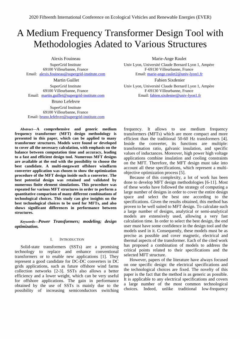
4) Thermal Network Resolution: The next step to establish the thermal network is to geometrically place the nodes of the network. A node must be present at each potential hotspot, and also at each surface because surfaces temperatures are required for convection and radiation calculation. The considered nodes of the thermal network for Core-Type geometry with air insulation are showed in Figure 5. Nodes for Shell-Type geometry are placed following the same pattern. In case of resin or air-resin insulation, there are additional nodes at the interfaces between windings and resin. Heat sources are localized on potential hotspot nodes, with a value corresponding to the integral of the loss density in a surrounding virtual block. Even though potential hotspots nodes are drawn at the centre of core cross-section and windings cross-sections, it may not be the case in reality. In fact, the position of the hotspot in the cross-section will depend on the surfaces temperatures as demonstrated in [27]. In (30), k is the thermal conductivity, q is the heat generation rate per volume unit, l is the distance between the surfaces, T1 is the temperature at the first surface (x=0), T2 is the temperature at the second surface (x=l) and xmax is the hotspot location.
lq
kTT
lxmax 12
2 (30)
Therefore, conduction, convection and radiation thermal resistances depend on surface temperatures, which are initially unknown. This is why an iterative resolution process must be performed to calculate thermal resistances. Temperatures at each node are calculated from the values of thermal resistances and heat sources, at each iteration. To solve this electrical equivalent network, numerical methods using admittance matrix inversion exist [31]. However, the electrical equivalent network is generally not too complex and can also be solved analytically using Kirchhoff’s circuit laws and Ohm’s law. Typically, it takes between five to ten iterations to converge. After convergence, maximal temperatures in each material can be easily obtained and compared with the maximal allowable temperature, thus allowing to keep or to exclude a design.
Fig. 5: Nodes of the thermal network for Core-Type geometry with air insulation (a) front view and (b) top view. Full circles represent potential hotspot nodes, half circles represents surface temperature nodes and dashed lines represent conduction paths
III. CASE STUDY
A. Definition of the Application
The case study considered is a DC-DC converter with a modular topology as described in [32], for a multi-megawatt converter in offshore windfarm application.
Magnetic Core Nanocrystalline Cut-Cores VITROPERM 500F
Windings Copper Litz cables
Insulation Oil MIDEL 7131 synthetic ester
Cooling Forced Convection – Oil temperature 40°C
The Table 2 summarizes the electrical specifications
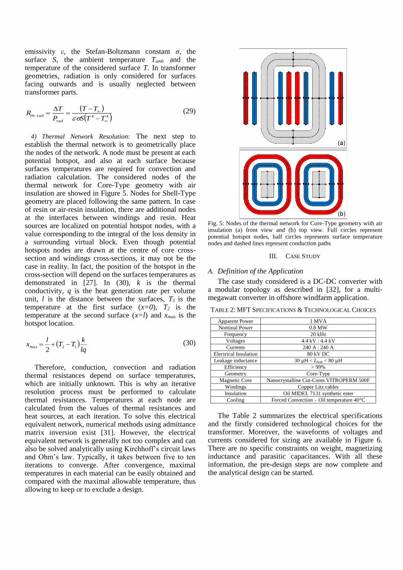
and the firstly considered technological choices for the transformer. Moreover, the waveforms of voltages and currents considered for sizing are available in Figure 6. There are no specific constraints on weight, magnetizing inductance and parasitic capacitances. With all these information, the pre-design steps are now complete and the analytical design can be started.
Fig. 6: Voltages and current waveforms applied to the transformer, the current is the same in both primary and secondary windings
B. Analytical Design
The first step of the analytical design is to gather the properties for each material: density, electrical conductivities, permittivity, dissipation factor, permeability, Steinmetz parameters, thermal conductivities, specific heat capacity, filling factors and maximum temperatures. Most of these data come from datasheet of manufacturers, but some of them such as the Steinmetz parameters were obtained from characterizations. Then, insulation distances between each part of the transformer are defined from the dielectric strength of the insulating material, taking into account an effective dielectric strength with a safety factor. For the oil used, it results in 20 mm insulation distance to withstand 80 kV DC.
The different degrees of freedom have been swept to cover the design space properly, and the calculation took 72 s for 1.5 million of designs, on a laptop with quad core CPU 2.4 GHz and 8 GB RAM, which is a common and accessible computing equipment. Filters were applied to the raw results to discard designs with too high temperatures. In this case, maximal allowed temperatures are 120 °C for both core and windings. The results of the analytical calculations are displayed in Figure 7. On this figure, the compromise between efficiency and volume can clearly be seen. All the points corresponding to a maximum efficiency for a given volume draw a Pareto front. It can also be seen that most compact designs have higher maximal temperature, as expected, reaching the limit value of 120 °C.
The Table 3 compares the performances of the optimization algorithm from literature and this work. It can be seen than most of the time dielectric aspects are not taken into account in other papers. Optimization methods are either genetic algorithm (GA), brute-force (BF), mesh refinement (MR) or manual (M). In terms of calculation time per design point, the method proposed here seems to be several orders of magnitude faster than the ones from literature, even if data is not always available in each reference. Also, when used, and calculation time is dependent on hardware.
Fig. 7: Efficiency, volume and maximal temperatures of 1.5 million design points.
TABLE 3: PERFORMANCES OF OPTIMIZATION ALGORITHMS
Reference work [5] [6] [7] [8] [9] [10] [11] This work
Leakage Ind.
Magnetizing Ind.
Core Losses
Windings Losses
Parasitic Capacitances
Dielectric Losses
Temperatures
Optimization Method GA BF BF MR GA M M BF
Total time (s) 180 10000 1800 72
No. points (thousands) 40 400 2000 1500
Time / design (ms) 4.5 5 0.05
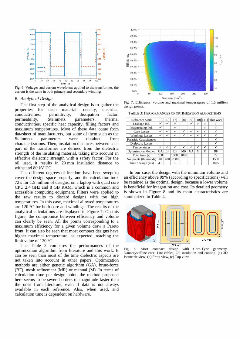
In our case, the design with the minimum volume and an efficiency above 99% (according to specifications) will be retained as the optimal design, because a lower volume is beneficial for integration and cost. Its detailed geometry is shown in Figure 8 and its main characteristics are summarized in Table 4.
Fig. 8: Most compact design with Core-Type geometry, Nanocrystalline core, Litz cables, Oil insulation and cooling. (a) 3D Isometric view, (b) Front view, (c) Top view
TABLE 4: MFT CHARACTERISTICS
Characteristic Analytical Value FEM Value Relative
Difference
Maximal induction 0.504 T - -
Number of turns 36:36 - -
Current density 9.58 A/mm2 - -
Strand number and diameter 3207 x 0.1 mm - -
Volume (box) 25.6 dm3 - -
Weight Core 18.7 kg - -
Weight Windings 7.9 kg - -
Weight Oil 18.6 kg - -
Total Weight 45.2 kg - -
Efficiency 99.60% 99.61% +0.97%
Core Losses 831 W 812 W +2.4%
Windings Losses 2183 W 2179 W +0.19%
Dielectric Losses 166 W 159 W +4.5%
Max. Core Temperature 118°C 126°C -10.0%
Max. Windings Temperature 116°C 117°C -1.4%
Magnetizing Inductance 14.4 mH 15.1 mH -4.7%
Leakage Inductance 37.5 µH 35.9 µH +4.5%
Primary-Secondary Capacitance 445 pF 424 pF +5.0%
Primary Capacitance 23 pF 32 pF -29.9%
Secondary Capacitance 32 pF 33 pF -4.6%
C. Numerical Validation
1) Inductances and Capacitances: Inductances are validated with a 3D Magnetostatic FEM study. Magnetic core, air gap and homogenized windings are considered. With this method, a magnetizing inductance of 15.1 mH and a leakage inductance of 35.9 µH were obtained. These values are in good agreement with the analytical ones with less than 5% deviation, and confirm the validity of the analytical models used. This is true because the designs have a low air gap value of 200 µm per gap (typical parasitic air gap value of nanocrystalline cut cores), and so fringing effect is limited. It is important that this condition is met to avoid additional losses due to fringing effect, in both magnetic core and windings.
The capacitance between primary and secondary windings was obtained with the same geometry (homogenized windings) and FEM software, but using an electrostatic solver. A parasitic capacitance of 424 pF was obtained, with again less than 5% deviation compared to the capacitance of 445 pF obtained analytically with (16). If edge effects were not taken into account, an analytical value of 414 pF would have been obtained. Therefore in this case, edge effects have a small impact on the parasitic capacitance value.
For parasitic capacitances of primary and secondary windings, the detailed geometry of windings must be considered. Therefore, 36 short-circuit turns for both primary and secondary windings were modelled. Parasitic capacitances of 32.5 pF and 33.0 pF were obtained with FEM simulations, respectively for primary and secondary windings. The difference is below 5% for secondary windings whereas it goes up to almost 30% for the primary windings. It shows that the model developed for parasitic capacitance of laminated cables
is only able to give a rough estimation in this case. However, the value of these capacitances is usually not a critical parameter in medium frequency transformer design so a rough estimation is acceptable. This deviation can be explained by the presence of magnetic core next to the primary winding which modifies the shape of electrical field in this area and therefore the values of non-consecutives turns parasitic capacitances (17). If edge effects and non-consecutive turns capacitances were neglected, the parasitic capacitances values obtained analytically would be 8.8 pF and 12 pF for primary and secondary windings, corresponding to an underestimation by three times of the parasitic capacitances. It shows that the developed model (18) increases significantly the accuracy in this case.
2) Losses: Magnetic losses cannot be directly and easily validated by FEM simulations from Maxwell equations because of the nature of static and dynamic hysteresis inside magnetic materials. An estimation of the loss density with IGSE (21) was performed by post-treating the results of a 3D magnetostatic simulation. The advantage of this method is that it does not require additional parameters, however it is only valid in the area where the magnetic material is used in its quasi-linear domain. By doing so, total magnetic losses of 812 W were obtained numerically, which is very close to the value of 831 W obtained analytically. The difference here can be explained by the non-homogeneous level of induction in the corners of the magnetic core which is not considered analytically.
Validation of windings losses is more about determining numerically the additional losses due to skin and proximity effects rather than to validate the DC Joules losses. Therefore, magnetoharmonics FEM simulations have to be performed. However, modelling a Litz cable is complex and this is why a 2D simulation was considered. The geometry is the winding window, because this is where the magnetic field is the most confined and therefore where the proximity effects will be the most important. The magnetic core acts as a symmetry plane for the magnetic field [19], and due to the symmetry of this geometry, only a quarter of the winding window is modelled. In our case, there are 3 207 strands per turn and a quarter of the winding window would therefore include more than 50 000 strands. Meshing all the details of this kind of geometry is far too complex. This is why an approach using homogenized cables for all turns except one has been used. Skin and proximity effects are only solved for this turn, while the other turns are present only to generate a correct surrounding magnetic field. Figure 9 shows the geometry used where it can be seen that the secondary winding is homogenized whereas the primary turns are not. Amongst the primary turns, only the ones located at
the middle and at the bottom of the winding were modelled in details with their strands structure. In fact, the magnetic field cartography is really different around the turns located at the bottom of the winding because this is where edge effects were expected and consequently proximity effects are different.
Fig. 9: Magnetic field cartography obtained with 2DFEM Magnetoharmonic simulation. (a) A quarter of the winding window. (b) Turn located at the middle of the winding. (c) Turn located at the bottom of the winding.
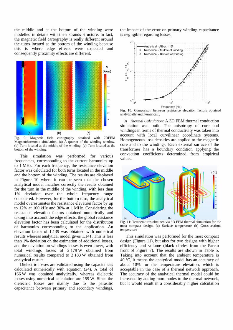
This simulation was performed for various frequencies, corresponding to the current harmonics up to 1 MHz. For each frequency, the resistance elevation factor was calculated for both turns located in the middle and the bottom of the winding. The results are displayed in Figure 10 where it can be seen that the chosen analytical model matches correctly the results obtained for the turn in the middle of the winding, with less than 1% deviation over the whole frequency range considered. However, for the bottom turn, the analytical model overestimates the resistance elevation factor by up to 12% at 100 kHz and 30% at 1 MHz. Considering the resistance elevation factors obtained numerically and taking into account the edge effects, the global resistance elevation factor has been calculated for the distribution of harmonics corresponding to the application. An elevation factor of 1.139 was obtained with numerical results whereas analytical model gives 1.141. This is less than 1% deviation on the estimation of additional losses, and the deviation on windings losses is even lower, with total windings losses of 2 179 W obtained from numerical results compared to 2 183 W obtained from analytical results.
Dielectric losses are validated using the capacitances calculated numerically with equation (24). A total of 166 W was obtained analytically, whereas dielectric losses using numerical calculation are 159 W. Since the dielectric losses are mainly due to the parasitic capacitance between primary and secondary windings,
the impact of the error on primary winding capacitance is negligible regarding losses.
Fig. 10: Comparison between resistance elevation factors obtained analytically and numerically
3) Thermal Calculation: A 3D FEM thermal conduction simulation was built. The anisotropy of core and windings in terms of thermal conductivity was taken into account with local curvilinear coordinate systems. Homogeneous loss densities are applied to the magnetic core and to the windings. Each external surface of the transformer has a boundary condition applying the convection coefficients determined from empirical values.
Fig. 11: Temperatures obtained via 3D FEM thermal simulation for the most compact design. (a) Surface temperature (b) Cross-sections temperature
This simulation was performed for the most compact design (Figure 11), but also for two designs with higher efficiency and volume (black circles from the Pareto front of Figure 7). The results are shown in Table 5. Taking into account that the ambient temperature is 40 °C, it means the analytical model has an accuracy of about 10% for the temperature elevation, which is acceptable in the case of a thermal network approach. The accuracy of the analytical thermal model could be increased by adding more nodes to the thermal network, but it would result in a considerably higher calculation
time, and the thermal calculation is already taking 70 s out of the total 72 s.
TABLE 5: MAXIMAL TEMPERATURES FOR THREE DESIGNS
Volume
(dm3) Efficiency
Core Primary Wind. Secondary Wind.
Model FEM Model FEM Model FEM
25.6 99.60% 118 °C 126 °C 116 °C 117 °C 112 °C 104 °C
50.0 99.76% 82 °C 88 °C 76 °C 76 °C 75 °C 71 °C
100.0 99.80% 69 °C 72 °C 54 °C 55 °C 56 °C 54 °C
A summary of the comparison of transformer main characteristics between values obtained analytically and numerically is available in Table 4. The deviation is acceptable for each parameter and therefore the transformer design is validated.
IV. TECHNOLOGICAL CHOICES AND FREQUENCY ANALYSIS
A. Technological Choices Comparison
Considering the application treated in paragraph III.A, other technological choices have been considered and studied following the same methodology. The goal here is to cover a lot of possible technological combinations to find the optimal one for this application. From the Table 1, all combinations of Core-Type Litz designs have been performed with either ferrite 3C93 or nanocrystalline Vitroperm 500F cut cores, which can both perform correctly up to 120°C. It allowed to compare the insulation and cooling technologies between them. From this study, it appears that some combinations of insulation and cooling technologies were very promising, whereas others were performing really badly in terms of both compactness and efficiency. Therefore, to reduce the number of cases to study, only the best insulation and cooling technologies were retained, that is resin insulation with air-forced or cold plate cooling and oil insulation with forced oil cooling. With this reduced set of insulation and cooling technologies, the shell-type and foil technologies were studied. In addition, some designs with high-performance SiFe steel sheets (JNEX900, 6.5% Si, 0.10 mm) were also considered for reference.
In total, 39 technological choices combinations were studied, and 8 of them were excluded due to temperature restrictions. Moreover, all designs with SiFe steel sheets had an efficiency below 99% and would therefore not respect the criteria defined for this application. The Table 6 shows the volume, weight and efficiency of the most compact designs for each technological choices combination. Results are sorted from most compact to less compact ones. The best design in terms of compactness is the Core-Type, Litz, nanocrystalline with oil for insulation and cooling, which was the one presented in details and numerically validated in section III.
TABLE 6: DESIGNS FOR VARIOUS TECHNOLOGICAL CHOICES
N° Geo. Cond. Mag. Ins. Cool. Volume (dm3)
Weight (kg)
Eff. (%)
1 CT Litz Nano. Oil OF 25.7 45.3 99.60
2 ST Litz Nano. Oil OF 27.2 57.6 99.60
3 ST Litz 3C93 Oil OF 30.5 74.7 99.70
4 CT Litz 3C93 Oil OF 30.8 59.2 99.66
5 CT Foil Nano. Oil OF 35.2 65.4 99.31
6 CT Foil 3C93 Oil OF 42.1 97.0 99.57
7 ST Foil Nano. Oil OF 50.9 327 99.05
8 CT Litz SiFe Oil OF 55.0 118 98.99
9 ST Foil 3C93 Oil OF 73.3 435 99.21
10 ST Litz SiFe Oil OF 74.3 153 98.55
11 CT Litz 3C93 Resin AF 85.4 184 99.74
12 ST Litz 3C93 Resin AF 98.8 252 99.75
13 CT Litz 3C93 Resin CP 108 205 99.79
14 CT Foil SiFe Oil OF 115 282 98.02
15 CT Litz Nano. Resin AF 115 227 99.55
16 ST Litz Nano. Resin AF 116 340 99.71
17 ST Litz 3C93 Resin CP 145 324 99.82
18 CT Litz Nano. Resin CP 158 325 99.70
19 ST Litz Nano. Resin CP 212 507 99.76
20 CT Foil 3C93 Resin AF 229 556 99.36
21 CT Foil Nano. Resin AF 244 541 99.14
22 CT Litz 3C93 Air AF 249 130 99.69
23 CT Litz 3C93 Resin AN 265 586 99.44
24 CT Litz Nano. Air AF 271 144 99.66
25 CT Litz 3C93 AR AF 280 139 99.72
26 CT Litz Nano. AR AF 303 136 99.62
27 CT Foil 3C93 Resin CP 323 661 99.19
28 CT Litz 3C93 Air AN 326 255 99.79
29 CT Litz 3C93 AR AN 355 242 99.79
30 CT Litz Nano. Air AN 398 380 99.75
31 CT Litz Nano. AR AN 425 352 99.73
32 CT Litz Nano. Resin AN No design <120°C
33 CT Litz SiFe Resin AF No design <120°C
34 CT Foil Nano. Resin CP No design <120°C
35 ST Foil Nano. Resin AF No design <120°C
36 ST Foil Nano. Resin CP No design <120°C
37 ST Foil 3C93 Resin AF No design <120°C
38 ST Foil 3C93 Resin CP No design <120°C
39 ST Foil SiFe Oil OF No design <120°C
CT: Core-Type, ST: Shell-Type, AR: Air-Resin, OF: Oil Forced, AF: Air Forced, AN: Air Natural, CP: Cold Plates.
Most compact designs have all in common to use oil insulation and cooling, which seems to be a prerequisite for this application if compactness is the most constrained property. Inside those solutions, Core-Type geometries seem to be slightly better than Shell-Type ones, Litz better than foil and nanocrystalline better than ferrite 3C93. As discussed before, SiFe solutions have a too low efficiency for this application, even though they can achieve quite good compactness.
However, oil solution may not be the best ones overall because of additional disadvantages like oil tank, pump management, complex manufacturing processes to ensure dry oil, maintenance, etc. Therefore another solution using dry-type insulation might be considered for these reasons even though the transformer designs give higher volumes. In this case, resin insulation with air forced cooling is the best combination, and nanocrystalline solutions fall behind ferrite ones. Core-Type is still better
than Shell-Type with a more noticeable difference, and Litz better than foil. Cooling using cold plates is behind air forced cooling, mainly because of the size of the cold plates in the total volume. Moreover, natural air cooling does not seem to have enough cooling power for this application. In the end, it shows that cooling is a crucial aspect of MFT design and therefore most designs, at least for this application, are limited by thermal reasons.
In this technological choices comparison, cost was not included. Material costs can be easily integrated into such a design tool, because the weight of each material is known. It would only require to make hypotheses on the costs per kilogram for each material (core, windings, solid and/or liquid insulation). Because such hypotheses are not constant in time, but following the market prices, we chose not to include it in this publication. Moreover, these costs would not include processing costs, which are harder to evaluate.
It should be noted that all these conclusions on technological choices are closely tied to the case study. However, the tendency should remain the same for applications within the same range of rated power, insulation and frequency. For applications with significant differences in the specifications, this study can be performed again with the new inputs in a limited time thanks to the automated design tool that has been developed.
B. Optimal Operating Frequency
For this application, an analysis of the dependence of transformer performances on operating frequencies has been performed. This analysis constitutes a modification of the specifications and is only for investigation purposes. Moreover, the optimal operating frequency will be given regarding only the transformer properties, and therefore is probably not the optimal frequency for the complete converter. A large frequency range from 1 kHz to 100 kHz is taken, and only the case Core-Type, Litz, nanocrystalline core with oil for insulation and cooling is considered. It is not said that this specific structure is the best one over this whole frequency range, and it is probably not the case. However, this analysis can still give good insights on the optimal operating frequency, especially in the case of small frequency variations around 20 kHz. The calculation was performed for 200 frequency points, and for each frequency, a total of 16.2 million designs were calculated to determine the optimal design for this frequency. The results in terms of volume and losses are presented in Figure 12. The first thing that can be seen on these figures, particularly on losses, is that there are some discontinuities in the curves. This is explained by the discretization of the design space: each degree of freedom can only take a value amongst predefined ones. To enhance the continuity of the curves, either a finer discretization or a more complex optimization algorithm must be used. However, these
curves are accurate enough to draw some conclusions. It appears that for this structure, the optimal operating frequency in terms of compactness is around 30-40 kHz. Above this frequency, both volume and losses start to increase, which means there is no need to increase the frequency to such levels with such technologies.
Fig. 12: Volumes and losses of most compact designs for each frequency, with Core-Type geometry, Nanocrystalline core, Litz cables, Oil insulation and cooling
This behavior is similar to the results found in [33-34] and reinforces the existence of an optimal operating frequency for MFTs. Moreover, the gain in compactness is much more important below 10 kHz than above. Because of the switching losses in converters, it may be better to work around 10 kHz instead of 20-40 kHz. Regarding losses, there is a significant decrease below 10 kHz for both core losses and windings losses, the dielectric losses being negligible for these low frequencies. However, above 10 kHz, total losses reach a plateau up to 40 kHz, from which losses start to increase mainly due to dielectric losses that increase rapidly for high frequencies.
V. CONCLUSION
A comprehensive medium frequency transformer design methodology was established to define the steps required to design MFTs, aiming to effectively cover a wide range of technologies. Based on this methodology, automated design tools were developed to cover the most common MFT technological choices and to be compatible with any voltage and current waveforms, and therefore with any converter topology, which is an evolution from the design methodologies found in the literature. This implementation was performed using models adapted to the MFT requirements, either from literature or from our own models [19]. Emphasis was placed on optimizing the computation time while meeting the required accuracy. This is especially true for the analytical thermal modelling because of its major importance in the MFT performances, which are most of the time thermally
limited, and its usually high computation cost. The developed design tool computed more than one million designs in about one minute with satisfactory accuracy, which is an improvement over the state of the art. Moreover, our approach took into consideration certain properties that are usually neglected or not considered such as parasitic capacitances and dielectric losses.
This methodology was applied to a realistic application corresponding to a DC-DC converter in the range of some megawatts, for offshore windfarm application. An optimal design was found thanks to the analytical design tool, and was verified by various FEM simulations. The results of the analytical and numerical models are in agreement, which constitutes a first validation of the models used. However, some improvements can be made to the parasitic capacitance calculations to take into account the presence of the magnetic core. Following this study on a specific MFT structure, a more global study was performed for a large number of possible combinations of technological choices. It demonstrated the potential of a multi-structure design methodology, and the large variations between structures that can lead to huge differences in performances. Therefore, in order to optimally design a MFT, this approach is necessary. Finally, a study on the performance of a specific structure over a wide frequency range was performed. It showed that there is an optimal frequency, beyond which it is useless to increase the frequency.
For future work, additional structure variants can be integrated into the design tool with the corresponding models to enable an even better multi-structure tool. Also, the use of an optimization algorithm instead of a complete discretization of the design space can be an improvement in some cases, for example when the MFT performance to be optimized is clearly defined or when trying to find an optimal operating frequency. However, discretization of the design remains a good first approach, as it provides a map of the possible designs and compromises. Finally, a comparison of calculation results following this methodology with experimental measurements on a manufactured MFT would be very useful to further validate the models. While it would be too costly to manufacture a prototype just to validate the models, a prototype manufactured for a more global project could be used in the future to validate the models.
APPENDIX A
The Table 7 below lists the correlations between dimensionless number, typically involving Nusselt number Nu, Prandtl number Pr and either Rayleigh number Ra for natural convection or Reynolds number Re for forced convection. Determining Nusselt number is equivalent to determine the convection coefficient. It also defines how the characteristic length (used in the
expression of some dimensionless numbers) can be calculated for each type of face, and the correlations being used for both natural convection and forced convection. For parallel plates, the channel width considered in the design tool is 10 mm.
TABLE 7: DIMENSIONLESS NUMBERS CORRELATIONS
Face type
Characteristic Length
Correlation
Nat
ura
l C
onv
ecti
on
Vertical Hot
Plate Plate height
3/1
4/1
13.0
59.0
RaNu
RaNu
if
if
9
9
10
10
Ra
Ra
Horizontal Hot Plate -
Top
Ratio plate area to plate
perimeter 3/1
4/1
15.0
54.0
RaNu
RaNu
if
if
7
7
10
10
Ra
Ra
Horizontal Hot Plate -
Bottom
Ratio plate area to plate
perimeter
4/127.0 RaNu
Vertical
Parallel Plates
Distance
between plates
5.0
5.02
873.2576
RaRaNu
Fo
rced
Conv
ecti
on
Plate Parallel
to Flow Plate length
4/1
3/2
2/13/1
0468.01
3387.0
2
Pr
RePrNu
if 510.5Re
871037.02
5/43/1 RePrNu
if510.5Re
Plate Face to
Flow
Half of plate
smallest dimension
3/12/1564.0 PrReNu
Plate Back to
Flow
Half of plate
smallest dimension
3/17.027.0 PrReNu
Parallel Plates
Duct
Twice the
distance between plates
3/18.0023.0
54.7
PrReNu
Nu
if
if
3
3
10.4
10.4
Re
Re
ACKNOWLEDGMENT
This work was supported by a grant overseen by the
French National Research Agency (ANR) as part of the
“Investissements d’Avenir” Program (ANE-ITE-002-
01).
REFERENCES
[1] J. W. Kolar and G. Ortiz., “Solid-state-transformers: key components of future traction and smart grid systems,” in Proceedings of the International Power Electronics Conference-ECCE Asia (IPEC 2014), 2014.
[2] A. Prasai, J.-S. Yim, D. Divan, et al., “A New Architecture for Offshore Wind Farms,” IEEE Transactions on Power Electronics, vol. 23, pp. 1198-1204, May 2008.
[3] T. Lagier, P. Ladoux, “A comparison of insulated DC-DC converters for HVDC off-shore wind farms,” in International Conference on Clean Electrical Power (ICCEP), 2015.
[4] J. E. Huber, J. W. Kolar, “Volume/weight/cost comparison of a 1MVA 10 kV/400 V solid-state against a conventional low-frequency distribution transformer,” in IEEE Energy Conversion Congress and Exposition (ECCE), 2014.
[5] A. Garcia-Bediaga, I. Villar, A. Rujas, et al., “Multiobjective Optimization of Medium-Frequency Transformers for Isolated
Soft-Switching Converters using a Genetic Algorithm,” IEEE Transactions on Power Electronics, vol. 32, pp. 2995-3006, 2016.
[6] M. A. Bahmani, T. Thiringer, M. Kharezy, “Optimization and experimental validation of medium-frequency high power transformers in solid-state transformer applications,” in IEEE Applied Power Electronics Conference and Exposition (APEC), 2016.
[7] M. Mogorovic, D. Dujic, “100kW, 10kHz Medium Frequency Transformer Design Optimization and Experimental Verification,” IEEE Transactions on Power Electronics, 2018.
[8] M. Leibl, G. Ortiz, J. W. Kolar, “Design and Experimental Analysis of a Medium-Frequency Transformer for Solid-State Transformer Applications,” IEEE Journal of Emerging and Selected Topics in Power Electronics, vol. 5, pp. 110-123, March 2017.
[9] P. Shuai, J. Biela, “Design and optimization of medium frequency, medium voltage transformers,” in 15th European Conference on Power Electronics and Applications (EPE), 2013.
[10] P. Huang, C. Mao, D. Wang, et al., “Optimal Design and Implementation of High-voltage High-power Silicon Steel Core Medium Frequency Transformer,” IEEE Transactions on Industrial Electronics, 2017.
[11] O. Aldosari, L. A. G. Rodriguez, J. C. Balda, et al., “Design Trade-Offs for Medium- and High-Frequency Transformers for Isolated Power Converters in Distribution System Applications,” in 9th IEEE International Symposium on Power Electronics for Distributed Generation Systems (PEDG), 2018.
[12] S. Vaisambhayana, C. Dincan, C. Shuyu, et al., “State of art survey for design of medium frequency high power transformer,” in Asian Conference on Energy, Power and Transportation Electrification (ACEPT), 2016.
[13] T. Kauder, K. Hameyer, “Performance Factor Comparison of nanocrystalline, amorphous and crystalline soft-magnetic Materials for medium-frequency Applications,” IEEE Transactions on Magnetics, 2017.
[14] S. Zhao, Q. Li, F. C. Lee, “High frequency transformer design for modular power conversion from medium voltage AC to 400V DC,” in IEEE Applied Power Electronics Conference and Exposition (APEC), 2017.
[15] M. Stojadinović, J. Biela, “Modelling and Design of a Medium Frequency Transformer for High Power DC-DC Converters,” in International Power Electronics Conference (IPEC-Niigata 2018 -ECCE Asia), 2018.
[16] M. Jafari, Z. Malekjamshidi, M. R. Islam, et al., “Modeling of magnetic flux in multi-winding toroidal core high frequency transformers using 3D reluctance network model,” in IEEE 11th International Conference on Power Electronics and Drive Systems (PEDS), 2015.
[17] S. Baek, S. Bhattacharya, “Analytical Modeling and Implementation of a Coaxially Wound Transformer with Integrated Filter Inductance for Isolated Soft-Switching DC-DC Converters,” IEEE Transactions on Industrial Electronics, 2017.
[18] G. Ortiz, J. Biela, D. Bortis, et al., “1 Megawatt, 20 kHz, isolated, bidirectional 12kV to 1.2kV DC-DC converter for renewable energy applications,” in 2010 International Power Electronics Conference (IPEC), 2010.
[19] A. Fouineau, M.-A. Raulet, B. Lefebvre, et al., “Semi-Analytical Methods for Calculation of Leakage Inductance and Frequency-Dependent Resistance of Windings in Transformers,” IEEE Transactions on Magnetics, vol. 54, pp. 1-10, Oct 2018.
[20] M. Mogorovic, D. Dujic, “Medium Frequency Transformer Leakage Inductance Modeling and Experimental Verification,” in IEEE Energy Conversion Congress and Exposition (ECCE), 2017.
[21] J. Biela, J. W. Kolar, “Using Transformer Parasitics for Resonant Converters - Review of the Calculation of the Stray Capacitance of Transformers,” IEEE Transactions on Industry Applications, vol. 44, pp. 223-233, Jan 2008.
[22] C. P. Steinmetz, “On the law of hysteresis,” Transactions of the American Institute of Electrical Engineers, vol. 9, pp. 1-64, 1892.
[23] I. Villar, A. Rufer, U. Viscarret, et al., “Analysis of empirical core loss evaluation methods for non-sinusoidally fed medium frequency power transformers,” in IEEE International Symposium on Industrial Electronics (ISIE), 2008.
[24] K. Venkatachalam, C. R. Sullivan, T. Abdallah, et al., “Accurate prediction of ferrite core loss with nonsinusoidal waveforms using only Steinmetz parameters,” in IEEE Workshop on Computers in Power Electronics, 2002.
[25] M. Albach, “Two-dimensional calculation of winding losses in transformers,” in IEEE 31st Annual Power Electronics Specialists Conference, 2000.
[26] P. L. Dowell, “Effects of eddy currents in transformer windings,” Proceedings of the Institution of Electrical Engineers, vol. 113, pp. 1387-1394, August 1966.
[27] D. Gerling, G. Dajaku, “Novel lumped-parameter thermal model for electrical systems,” in European Conference on Power Electronics and Applications (EPE), 2005.
[28] P. A. Kyaw, J. Qiu, C. R. Sullivan, “Analytical Thermal Model for Inductor and Transformer Windings and Litz Wire,” in IEEE 19th Workshop on Control and Modeling for Power Electronics (COMPEL), 2018.
[29] W. M. Rohsenow, J. P. Hartnett, Y. I. Cho, et al., “Handbook of heat transfer,” vol. 3, McGraw-Hill New York, 1998.
[30] M. Favre-Marinet, S. Tardu, “Convective Heat Transfer: Solved Problems,” John Wiley & Sons, 2013.
[31] M. Mogorovic, D. Dujic, “Thermal Modeling and Experimental Verification of an Air Cooled Medium Frequency Transformer,” in 19th European Conference on Power Electronics and Applications (EPE'17 ECCE Europe), 2017.
[32] J. Maneiro, R. Ryndzionek, T. Lagier, et al., “Design of a SiC based triple active bridge ceil for a multi-megawatt DC-DC converter,” in 19th European Conference on Power Electronics and Applications (EPE'17 ECCE Europe), 2017.
[33] U. Drofenik, “A 150kW Medium Frequency Transformer Optimized for Maximum Power Density,” in 7th International Conference on Integrated Power Electronics Systems (CIPS), 2012.
[34] M. Mogorovic, D. Dujic, “Sensitivity Analysis of Medium Frequency Transformer Designs for Solid State Transformers,” IEEE Transactions on Power Electronics, 2018.