AN ABSTRACT OF THE THESIS OF William Andrew Mittelstadt for the Master of Science (Degree) (Name of student) in Electrical Engineering presented on (Major) Title: A Method of Improving Power System Transient Stability Using Controllable Parameters Abstract approved: John L. Sauge Controllable parameters in a power system include genera- tor terminal voltage, generator input power and network ad- mittances. These parameters can be controlled to damp mechanical rotor oscillation in the generators and thereby improve system transient stability. Explicit equations are derived in this thesis for the control of these parameters to introduce damping uniformly throughout a large power system. These equations are derived on the basis of minimizing a positive definite error function. Decision functions are included which inhibit damping action when it leads to system instability. This method can be used to coordinate the appli- cation of locally based damping techniques. A three - generator example is presented illustrating the damping method. ff^f
Transcript
AN ABSTRACT OF THE THESIS OF
William Andrew Mittelstadt for the Master of Science (Degree) (Name of student)
in Electrical Engineering presented on (Major)
Title: A Method of Improving Power System Transient
Stability Using Controllable Parameters
Abstract approved:
John L. Sauge
Controllable parameters in a power system include genera-
tor terminal voltage, generator input power and network ad-
mittances. These parameters can be controlled to damp
mechanical rotor oscillation in the generators and thereby
improve system transient stability. Explicit equations are
derived in this thesis for the control of these parameters to
introduce damping uniformly throughout a large power system.
These equations are derived on the basis of minimizing a
positive definite error function. Decision functions are
included which inhibit damping action when it leads to system
instability. This method can be used to coordinate the appli-
cation of locally based damping techniques. A three - generator
example is presented illustrating the damping method.
ff^f
A Method of Improving Power System Transient Stability
Using Controllable Parameters
by
William Andrew Mittelstadt
A THESIS
submitted to
Oregon State University
in partial fulfillment of the requirements for the
degree of
Master of Science
June 1968
APPROVED:
Associate P4.fessor of Electri1al & Electronic Engineering in charge of major
Head .f Department of El ctrical & Electronic Engineering
Dean of Graduate School
Date thesis is presented
Typed by Clistie Stoddard for William Andrew Mittelstadt
r
ACKNOWLEDGMENT
I wish to express my sincere and grateful appreciation
to Dr. John L. Saugen for introduction to key system concepts
pertaining to this thesis and for constructive criticism in
the preparation of the manuscript. Special thanks are also
in order to Professor John F. Engle for practical insight into
power system needs.
Appreciation is also extended to my associates at
Bonneville Power Administration for encouraging this work,
with special gratitude to Richard E. Rose for assistance in
digital computer programming.
TABLE OF CONTENTS
I. Introduction 1
Introduction 1
Statement of the Problem 2 Power System Model 2 Controllable Parameters 6 The Fundamental Error Quantity 7
The Fundamental Error Function 8
Measurement of the Fundamental Error Quantity 9
Statement of Results 12 Discussion of Results 14 Recommendation for Further Study 16 Literature Review 16 Nomenclature 19
II. Derivation of Damping Equations 23 Expansion of 0 23 W. Control Equation 25 G. Control Equation 28 E. Control Equation 32 dl(Y. B. ) /dt Control Equation 37
ij ij
III. The Damping Method Applied to a Three - Generator Model 39
Model System 39 Simulation Program 42 Reference Case 45 Voltage Control Damping Cases 45 Dynamic Braking Case 52 Prime Mover Control 56
Bibliography 57 Appendix A 59 Appendix B 62 Appendix C 65 Appendix D 67
LIST OF FIGURES
Figure Page
1. One -Line Diagram 3
2. General Positive Sequence Model 5
3. Approximate Differentiator Circuit for Estimation of á 10
4. Block Diagram of a Method for Approximating E. 11
5. Principal Equilibrium Points for the Undamped Three -Generator Model of Chapter III 27
6. Dynamic Braking Following a Simple Power System Disturbance 33
7. Dynamic Braking Applied Following a -r Second Delay Allowed for Attempted Line Reclosure 34
8. Positive Sequence Diagram of the Three - Generator Model System 40
9. The Undamped Three -Generator Reference Case 46
10. Total Voltage Control Applied to the Three - Generator Reference Case 48
11. Local Voltage Control Applied to the Three -
Generator Reference Case 49
12. The Voltage Response of Each Generator with Local and Total Voltage Control Applied to
the Three -Generator Reference Case 51
13. Dynamic Braking Applied to the Three - Generator Reference Case 54
14. Response of E. with Dynamic Braking Applied to the Three- Génerator Reference Case 55
A METHOD OF IMPROVING POWER SYSTEM TRANSIENT STABILITY
USING CONTROLLABLE PARAMETERS
I. INTRODUCTION
Introduction
To meet the growing demand for economical power, distant
regions are interconnected electrically. A good example is the
B. C., and Seattle to Los Angeles and Phoenix, in-
cluding the biggest hydro system in America (the
Bonneville Power Administration system), the biggest
municipal system (Los Angeles Department of Water and Power), and one of the biggest private systems (the
private utilities of California).
As a power system grows, the difficulty of withstanding
unexpected disturbances without disintegration increases.
Immediately following a disturbance, mechanical oscillation
occurs in each generator relative to a reference axis rotating
at nominal shaft speed. The rapid extinction of this oscilla-
tion, which is called damping, improves the system's ability
to remain intact.
Transient stability is a condition which exists if a dis-
turbance does not cause power system disintegration. The addi-
tion of damping will improve transient stability to include an
enlarged class of system disturbances.
2
It is desirable that the mechanical oscillation of every
generator be given a nearly equal rate of damping since system
separation can occur if a single machine (generator) remains
undamped. Uniform power system damping is that condition which
exists if equal damping is given to every machine oscillation.
Several techniques which introduce damping at local points in
the power system are cited in the Literature Review. A method
of coordinating these techniques is necessary to provide uniform
system damping.
A method is presented in this thesis governing the control
of basic power system parameters to improve transient stability
with nearly uniform damping. The method can be employed to
coordinate local damping techniques.
Statement of the Problem
Power System Model
Power systems are basically composed of a set of generating
plants, a distribution network and a combination of industrial,
commercial and residential loads. An example of a partial power
system is given in Figure 1. In this diagram, a single line
represents a full three phase transmission tie. E.LA. is the
effective phase -to- neutral voltage and phasor angle of the ith
machine.
Trans or rner
To Main System
Buslk 1 Indust ri 4( Load
Res iGlen +i4 load
Figure 1. One -Line Diagram.
Genera ator
w
Bus #w2
A positive sequence network model is used in this thesis as
given in Figure 2. The positive sequence network representation
is satisfactory when balanced loading appears on all three elec-
trical phases. Under unbalanced conditions, the zero and nega-
tive sequence networks must also be employed. Power system
disturbances can occur in balanced or unbalanced form. The
positive sequence form can be used for damping purposes when the
disturbed transmission line is removed quickly by circuit breaker
action.
The "dynamic swing equation" which describes oscillation of
the ith generator for a system composed of N generators is
where
Md = W. - P. - C.d. i i i i i i
d. = the angular rotor displacement from a synchronously
1 rotating reference axis,
M. = the generator inertia constant,
W. = the mechanical input power to the ith machine minus
1 all generator and prime mover losses,
Ci = the internal generator damping coefficient
and the electrical power output Pi is given by
N
Pi i.
= E.2G. + 1:E.E.Y. B. j . j
j.1 where
N
G. = yjCos eij, j=1
Yij L Tij = -U Leij for
(1 )
(2)
4
i
1 1 1 j
i
(3)
j, (4)
Wi yiiLeíi
%i Le»
Figure 2. General Positive Sequence Model.
\JI
Wi
and
W. Cos (T. - 'j lj
+ A.) J
Jij L ei.
= a network admittance resulting from J delta -star simplification.
The terms W., E. and G. can be independently controlled to
introduce power system damping. This thesis provides the de-
velopment of explicit equations for the control of W. , E. and
Gi to give nearly uniform power system damping. This work pro-
vides the basis for the coordinated application of local damping
techniques.
Controllable Parameters
Local damping techniques, which are cited at the end of this
chapter, can be shown to control W., i G, E.
i j and Y L T .
i j i i Each power system generator has a system for controlling the
mechanical input power which is Wi plus all mechanical and
electrical machine losses. Since these losses are on the order
of one per cent, damping action which controls the mechanical
input power also controls W.. Each generator also has an
excitation system which is normally used to regulate the terminal
voltage Ei . A supplementary signal may be introduced to control
E. to give power system damping.
Dynamic braking is a damping technique which involves the
temporary application of special dissipative loads called braking
Y.. L T.. O ,
11 11
A. 1
= (5)
= (6)
(7)
7
resistors and the limited removal of consumer loads for short
periods which is called load shedding. Dynamic braking is
principally reflected in the model presented as step changes in
G.. i
Damping may be obtained by the switching of series capaci-
tors in transmission lines which is reflected in the model as
step changes in Yid L T... No equation is developed for the
control of Yid L Ti., however, since step changes in this
parameter do not uniquely define switching operations in the
real system.
The Fundamental Error Quantity
To obtain uniform damping it is desirable to employ the
angular acceleration of each generator (d) as a controlling
error quantity. By this choice,equal emphasis is given to
machines of large or small generating capacity. The "dynamic
swing equation" may be written as
i
W. . - p . =
M. i
i
Since internal generator damping is light, the right side of
equation (8) represents a good approximation of Ó, and is
defined as the fundamental error quantity Ei .
Thus
Ei M.
i
(8)
(9)
i
d Ci
i +
A W. - P = i i
When the magnitude of Ei is large, it closely approximates Si,
and forcing Ei toward zero also results in forcing toward
zero. As the magnitude of Ei becomes small, equation (8) may
be approximated by
Ci ól = o (lo) M.
i
which has a stable solution for bi of
*Si = k. exp ( -C.t/M.) i and for it of
ó = - Ci exp ( - C i t/M
i )
i M. i
where Ci /Mi must be positive.
(12)
Thus for large and small magnitudes of Ei , control action which
forces E, to zero also forces the system to a stable equilibrium i
condition.
The Fundamental Error Function
The fundamental error function is defined as
N
1 = 2E
2 i
i=1
This positive definite function is employed to determine regula-
(13)
tion of controllable parameters which gives uniform power system
damping. The time derivative of equation (13) is
6
8
N . . .
= E Ei (Wi - Pi ) 1
j=1 M. i
9
If all components of are continuously negative, 0 asymptoti-
cally approaches zero which implies that E. approaches zero
also. Explicit equations are derived in Chapter II which cause
as many terms of to be negative as possible.
Measurement of the Fundamental Error Quantity
To apply the damping control equations which have been de-
veloped, E. must be measured at each generator in the power
system. Currently rotor angular acceleration, b , is estimated i
by using the approximate time derivative of generator frequency
as given in Figure 3 (5, 11). These devices are used on a
limited scale for damping low frequency tie -line oscillations.
The response of this instrumentation system is limited by the
slow frequency transducers.
Blythe has presented a method for estimating Ei as given
in Figure 4 (2).
Under transient conditions, P. oscillates about W.. By
employing the filter, G (s), the highest oscillation frequencies
are attenuated, thus giving an approximation of W.. The esti- i
mated E, is the difference between the approximate W. and P..
Although Blythe used a first order filter of time constant
high order forms may also be used. To measure P., a high speed
power transducer must be used. Although a high speed power
(14)
;$
/p ,
Approxir+wte. Cont rolled Gain Different i at o r
A A Awpler
f t
Hi. l, GoVt Ampli -Piers
Figure 3. Approximate Differentiator Circuit for Estimation of d
r O
., Si
.3,.0
-
Pi GCS)
G(s) _
i
Figure 4. Block Diagram of a Method for Approximating Ei.
Ei
Ol Wi
I + o.S
12
transducer is considered to have lower accuracy than the slow
responding thermocouple model, no difficulty is expected since
only the relative magnitude of E. is necessary.
Statement of Results
Explicit equations governing the control of W., G. and E.
are now given. The expression for W. control is
where
and
W. _ - YM. (y i E.
Y= a positive system coefficient
for di Ei I /dt < 0
O for dIEi I /dt i 0
The general expression for G. control is
Where
Mi Ei 2
E. i
) = a positive system coefficient.
For discretely operated controllers this becomes
(31)
(30)
(34)
i = 1
.
where
and
6 NOin iUu ( t-Ti )
1 E 2
E.> 0
-1 E.<O i and AG.E 2/M. < IEiI
i i i
O AGiEi /Mi> IEiI
U (t o
-T.) = a unit impulse occurring at t = T. i i
AG. = the magnitude of the change in G..
The term Ti is defined as the time at which IEiI reaches a
maxima.
The general expression for Ei control is
where
and
= p Soi Ei
E Ri + Li
13
(43)
(44)
(52)
}L = a positive system coefficient,
£ Ri E.Y.
(BiJ + BJi EJ ) , (46)
J=1 Mi El
B.. Cos (T.. - A. + A.) (6) ij ij i J
Li 4 2 EiGi
M. i
(45)
i
JL. 1
1
1
J
- _
{ Ilillll
r
=
1
The form may be reduced to
E _ i p SGi Ei
ELi
14
(53)
at generators having a relatively large driving point conduct-
ance, Gi . An expression controlling Y. lj ij
L T is not presented
since its interpretation in the actual network is not unique.
Discussion of Results
The equations presented may be used explicitly to govern
the application of local damping devices. It is not necessary
that the parameter responses exactly follow the given equations
although sign agreement should be maintained.
All control equations are based around the fundamental
error quantity Ei. A practical method of estimating this
quantity is given on page 9.
The equation for control of Wi is the simplest of those
given. Furthermore, this parameter is the most desirable to
employ for system damping since it does not directly introduce
voltage fluctuation (as does Ei control) and it does not re-
quire temporary dropping of any customer loads (as can G.
control). Unfortunately, this is the most difficult parameter
to control in practice because of the slow response of the
generator and turbine systems.
Some success has been achieved by Schleif, Martin and
Angell for low frequency oscillations (11). Fruitful ideas
1
15
leading to rapid control of W. are highly desirable.
The equation for control of G. may be directly employed in
the application of dynamic braking. This provides the solution
to the three primary difficulties:
1. Relative brake resistor sizes are given for each
generating plant by equation (35).
2. The time of application is given for each switching
operation in terms of a locally measurable parameter.
3. A decision function is provided by equation (42) to
determine when braking operations must be terminated.
It is most desirable if braking resistors are applied at the
generator sites. If load shedding is employed, it must be
determined which loads within the system selectively influence
the driving point conductances.
With the introduction of improved exciter systems, the
control of E. has become a reasonable method of introducing
damping. Two equations are given for the control of E, of
which one requires the knowledge of many system parameters, and
the other, only local parameters. From the three -generator
example of Chapter III, it was found that the local equation gave
results almost as satisfactory as the total system equation.
By examination of equations (45) and (46) it appears that
generators with large driving point conductance values are most
amenable to the local voltage control equation.
16
The derived equations give instruction for the control of
Wi, Gi and Ei to obtain nearly uniform power system damping.
Further extension of this method is intended by the author.
Recommendation for Further Study
The following topics are recommended for further study:
1. The extent of applicability of the local voltage
control equation should be determined.
2. Further work should be conducted on circuits for
rapid measurement of the fundamental error quantity,
E.. i
3. The most desirable range of system coefficients LIN
and u should be determined.
4. Procedures should be prepared for determining how
shed loads influence G.. i
5. The damping method should be simulated on a large
power system model.
Literature Review
The subject of power system transient stability is very
active in the literature. Methods have been proposed for de-
termining the boundary region of system stability using the
direct method of Liapunov. Other emphasis has been on locally
controlled damping techniques.
17
By the direct method of Liapunov, a positive definite
(always positive) function V is defined in terms of system state
variables. The time derivative V may be explicitly determined
by using the system differential equations. Asymptotic sta-
bility of the system response is guaranteed over the region for
which V is always negative.
Tf a good Liapunov function is chosen, the negative region
of V closely corresponds to the true region of system stability.
Liapunov functions have been derived for several degrees of re-
finement (3, 6, 17). A useful resulting concept is the deter-
mination of the maximum time within which a disturbance must be
cleared to maintain stability (3).
The local damping techniques presented are intended for
"on- line" operation. Much work has been done by Schleif of
the U. S. Bureau of Reclamation on damping by prime mover con-
trol. This work was prompted by serious oscillations in
Northwest -Southwest tie lines through Utah and Colorado. Fre-
quent line tripping occurred as a result of drifting tie -line
load and periodic swings at six cycles per minute (5). The
work by Schleif has resulted in prime mover control at Grand
Coulee and McNary dams based on the time derivative of local
frequency (11, 12). Satisfactory damping of low frequency
tie -line oscillations was obtained.
The introduction of damping by generator terminal voltage
control has received interest because of the low modification
18
cost. The generator voltage may be controlled by changing the
current of the field winding located on the rotating generator
shaft. The exciter system which provides the field winding
current must be driven to high voltage magnitudes to give a
rapid change in generator terminal voltage. Techniques of
bang -bang (discrete output) exciter control have been developed
by O. J. M. Smith and G. A. Jones (7, 13). Smith uses local
shaft angle, shaft velocity, field current and power flow as
inputs to decision making controllers which command exciter
voltage to be maximum positive, maximum negative, or normal.
Much work has also been done by Blythe on generator
voltage control of the Peace River Transmission System in
Canada. Preliminary digital simulation studies were conducted
using frequency deviation from nominal 60 cycles per second as
a control signal (4). Blythe and Shier have also given a
comparison of damping possible with rotating and static
(thyrister) excitation systems. The static exciter gives a
significant improvement in the ability to control terminal
voltage for this purpose (2, 16).
A damping technique which has received much discussion pro
and con is dynamic braking (10). Although the application of
discrete braking resistors is considered by some to be a drastic
measure, others maintain that this is necessary for the severe
oscillations which may occur in interconnected systems. It has
been suggested that damping resistors may be applied for one to
19
one and one -half seconds following a disturbance (4). The
feasibility of employing braking resistors is being considered
by Bonneville Power Administration.
The switching of series capacitors is being employed in
the Pacific Northwest -Southwest Intertie (15). The insertion
of series capacitors in transmission lines increases line
admittance which may be used to improve transient stability
(8, 10). One plan of application is to insert series capacitors
immediately following a disturbance and leaving them in until
system conditions return to normal operation. Another method
is to insert series capacitors when the electrical phase angle
between transmission line terminals is increasing and removal
of capacitors when the angle is decreasing (10).
Nomenclature
English Symbols
A. = the phase angle of the phase -to- neutral voltage for the
ith generator, in radians.
B. j
= a variable defined by equation (6).
C. = the internal damping coefficient for the ith generator,
in per -unit power second /radian.
E. = the magnitude of the phase -to- neutral voltage of the ith
generator, in per -unit voltage.
.* E. = the value used for E. in the Runge Kutta numerical inte-
i i gration subroutine, in units of per -unit voltage /second.
1
1
1
20
£Li = the local voltage control variable defined by equation
(45).
£Ri = the remote voltage control variable defined by equation
(46).
E = the exciter voltage of the ith generator, in per -unit xi
voltage.
G(s) = a transfer function.
G. = the driving point conductance of the ith generator de-
fined by equation (3), in per -unit admittance.
AG. = the magnitude of the change in G. resulting from
dynamic braking.
GNi = the nominal value of G. when dynamic braking is not
applied, in per -unit admittance.
Ifi = the d.c. field current of the ith generator, in per -unit
current.
K. = a generator model constant.
k. = a constant of integration.
Lfi = the inductance of the field winding of the ith generator.
M. = the inertia constant for the ith generator, in per -unit
power second2 /radian.
N = the number of generators in the power system.
Pi = the electrical power output of the ith generator given
by equation (2), in per -unit power.
Q. = a Runge Kutta vector defined by equation (61).
R. = a Runge Kutta vector defined by equation (62).
i
i
i
i
i
1
i
21
Rfi = the field winding resistance of the ith generator, in
per -unit resistance.
Si = a Runge Kutta vector defined by equation (63).
T. = the time at which a dynamic braking switching operation
occurs, in seconds.
T. = the phasor angle of the transfer admittance defined by ij
equation (4), in radians.
Vi = a Runge Kutta vector defined by equation (64).
W. = the mechanical input power to the ith generator minus
all generator and prime mover losses, in per -unit power.
Xi a Runge Kutta vector defined by equations (57) and (60).
Y. = a transfer admittance magnitude defined by equation (4), ij
in per -unit admittance.
an admittance magnitude resulting from delta -star net-
work reduction, in per -unit admittance.
a variable defined in equation (28).
Greek Symbols
i
Y
a coefficient used in the development of the Wi control
equation.
a coefficient used in the development of the Ki
control
equation.
-1. = the system coefficent for control of W., in seconds
i
i
=
yij =
3 =
cl. =
=
ai
Ei
Ei
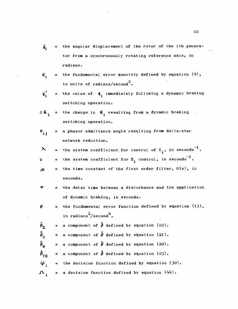
22
= the angular displacement of the rotor of the ith genera-
tor from a synchronously rotating reference axis, in
radians.
= the fundamental error quantity defined by equation (9),
in units of radians /second2.
= the value of Ei immediately following a dynamic braking
switching operation.
A Ei = the change in Ei resulting from a dynamic braking
switching operation.
9. = a phasor admittance angle resulting from delta -star ij
network reduction.
= the system coefficient for control of Gi , in seconds -1.
= the system coefficient for E. control, in seconds -1.
= the time constant of the first order filter, G(s), in
seconds.
?' = the delay time between a disturbance and the application
of dynamic braking, in seconds.
0 = the fundamental error function defined by equation (13),
in radians2 /second4.
E = a component of Th defined by equation (22).
0G = a component of ¢ defined by equation (21).
fów = a component of jó defined by equation (20).
YB = a component of defined by equation (23).
(/ii = the decision function defined by equation (30).
11. = a decision function defined by equation (44). i
T
11 1
Ap
Q
23
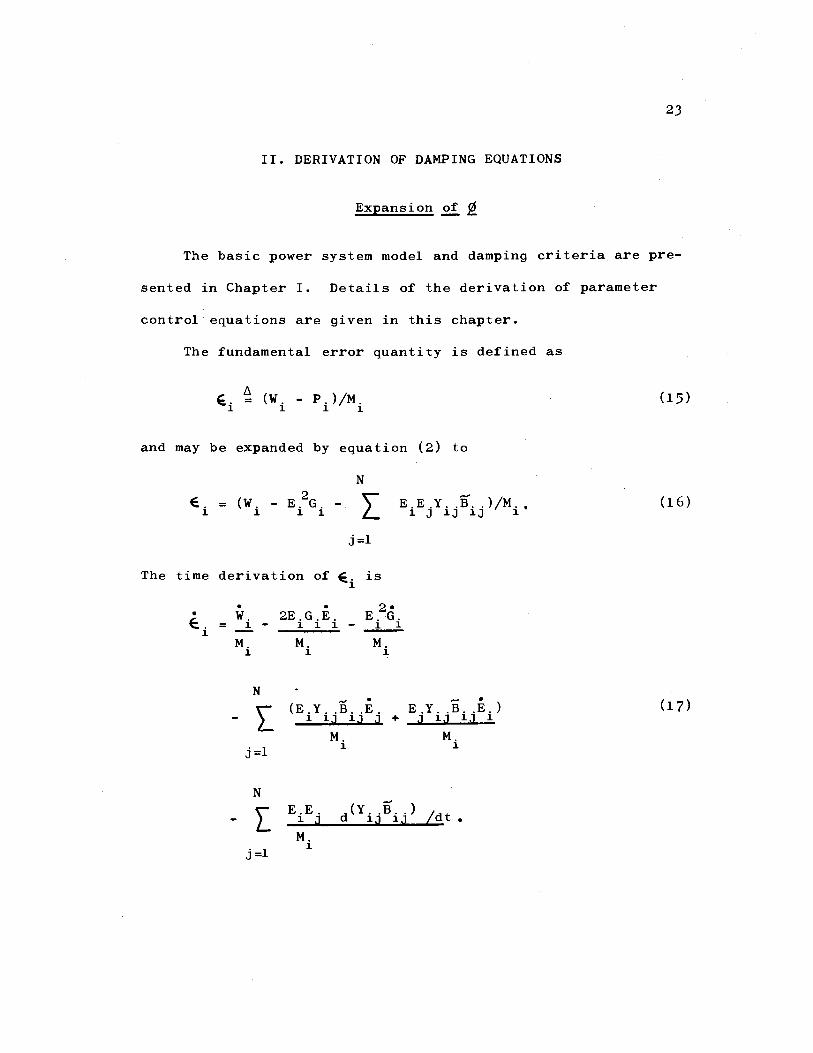
H. DERIVATION OF DAMPING EQUATIONS
Expansion of g
The basic power system model and damping criteria are pre-
sented in Chapter I. Details of the derivation of parameter
control equations are given in this chapter.
The fundamental error quantity is defined as
A ei = (w. - Pi)/Mi
and may be expanded by equation (2) to
N
Ei = (Wi - E. G.
2 - E E.E.Y.
i=1
The time derivation of E is i 2
. W. 2E.G.E. E.G. E . = i - 1 1 1 - i i -
M. M. M. i i i
N N
(EiYijBijEj EjYijBijEi)
M. M. i i j=1
N
- 1: EiEj d(Yijij) /dt. M. i
i=1
(15)
(16)
(17)
1
+
The time derivative of the fundamental error function is
N
;J= E EiÉi i=1
which may be expanded by equation (17) to give
where
and
. . . . = W + G + E
N
E iwi W
M.
i=1
N
0 r E2.G. -i i i i=1
24
(18)
(19)
(20)
(21)
N N
E E 6i 2EiGi + sYij (Bi + B.i E1 )Ei) (22)
M. M. Ei i=1 1 j=1 i
N N
OYB - E ei E E.E. d(Yi Bi )/dt .
M. i=1 j=1 1
(23)
The basic plan is to control the parameters W., G. and E. to
force ;$ to be as negative as possible.
.
Qí
G -
-
25
W. Control Equation
It can be shown by equation (20) that ßíW is always negative
if W. is defined as i
W. = - of. i Ei (24)
where d. is a positive coefficient. Control action is applied
equally to all generators having equal E if oCi is defined as
(25)
where Y is a positive coefficient. The resulting equations for
0W and Wi are
and
N
ó E 2
i=1
w. = -Y M. E i
(26)
(27)
It may be shown by substitution of equation (27) into equation
(1) that this action acts continuously to reduce angular accel-
eration of ó at each generator. Strictly from the standpoint i
of damping oscillation this action is desirable, but in terms of
transient stability, a further modification is necessary.
This modification is a result of consideration of power
system equilibrium points. El -Abiad and Nagappan have derived
.
C. °= YM.
26
equations for estimating stable and unstable equilibrium points
(3). The relative rotor angle of a stable equilibrium condition
between the ith and jth machine is approximately
where
(bi - ój) = Sin -1 (
M.W. - M.E. 2 G. + M.E.
2 G.
1 1 1 J J
(M, + M.) E.E.Y. ,Sin(T. .) 1 J 1 J 13 1J
and the unstable condition is given by
= (ai - a) 1r - Sin -1 (3) .
By examining the principal angles of Sin -1
(i), it may be
shown that for a stable system equilibrium point,the angles
(28)
(29)
(di .- ,S.) should lie within + 90 degrees. An unstable equilib-
rium condition exists if any (a, - b,) lies between 90 and 270 1 J
degrees. Figure 5 illustrates the set of principal equilibrium
points for the three -generator system considered in Chapter III.
It is desirable that damping action does not drive the
relative system angles toward the region of unstable equilib-
rium points since stability may be lost. For this reason, the
retarding angular acceleration should not be diminished when
d 1 E iI is positive.
dt
The derivation of the W. control equation is complete with 1
the addition of
M.W. - 3.= j 1 1 J i
27
200
u) u u 160 L,
¢
C 120
yo
go
Unsi able poets
40
StaLls point
O 0 40 SO 12.0 160 200
Sa - 83 in Degrees
Figure 5. Principal Equilibrium Points for the Undamped Three -Generator Model of Chapter III.
9-
, . a
^ó
i A = 1
0
for
for
dt.l /dt
d E.) /dt
<
>
O
O
thereby giving
= M.
Gi Control Equation
28
(30)
(31 )
It can be shown by equation (21) that 0G
is always negative
if G. is defined as i . p
Ei (32)
where /3 is a positive coefficient. Control action is applied
equally to all generators having equal E , if i
is defined as
A M. ) /3i =
E2 i
(33)
where ) is a positive system coefficient.
In equation (33), E can be approximated by its nominal i
value since deviations from the nominal value are generally
small.
The technique of dynamic braking appearing in the literature
involves step changes in G. rather than continuous control as
given by
i -
(
i
,
Gi = /3 i
G. = i .
x E E i
29
(34)
To provide for discrete changes in Gi ,a unit impulse term
Uo(t -Ti) is employed which occurs when the argument t -Ti is
zero. If only one size braking resistor is available at each
generation site, the magnitude should be determined by
AG = Miñ
E2 i
(35)
where the nominal terminal voltage is used for E.. With a fixed
magnitude discrete braking operation,the resulting change in
0G is given by
AOG = U_I(t-Ti) (36)
where U_1(t -T.) is the unit step occurring at t= T..
It can be seen from equation (21) that a maximum decrease in
0G is sustained if the switching occurs when IEiA is at a maxi-
mum value. Studies have indicated that it is desirable to apply
dynamic braking immediately following a disturbance (4). This is
compatible with the maximum IE..I criterion since IE.I always
reaches a maxima immediately following a disturbance.
Since a switched or discretely controlled operation is
employed, it is necessary to develop a criterion to distinguish
when dynamic braking should be applied and when it should be
i
-N
30
discontinued following an application. If a switching opera
tion will result in a reversal of the sign of E , following a
fault, no switching action is taken. Furthermore, dynamic
braking is discontinued following a sustained application if
further switching will result in a reversal of the sign of E ..
To determine the switching criterion, equation (2) is
substituted into equation (9) giving
N
= 1 (W. - E 2G - E.E.Y. jBij)
M. i 1 i 1
1 j=1
(37)
The term iG. is added to G. if a braking resistor is applied, 1 1
and is substracted from G. if load shedding occurs. Immediately
following a switching operation, equation (37) becomes
N
E'. = 1 (W. - E 2 (G. + AG) - E.E.Y. B. ) 1 ly 1 1 1 1 j lj ij
1 j=1
(38)
where Ei is the resulting fundamental error quantity. The
change in Ei, 1E., is
AEi - Ei - Ei - E . 2AG
= + 1 1 .
M. 1
(39)
The braking resistor is applied when E. reaches a maximum
positive value providing a sign reversal of E will not occur.
Thus if the inequality
1
i
Ei
y
I Eil -
E 2aGi
M. i
31
(40)
is satisfied, a braking resistor may be applied. Load shedding
may be applied when E. reaches a maximum negative value if a
sign reversal of Ei does not result. Thus, if the inequality
2 EAGi - IE.I + <
M
(41)
is satisfied, load shedding may be applied. By inspection it is
seen that equation (40) and equation (41) are the same inequality
and may be written as
L E I > Ei AGi
M.
(42)
and is called the dynamic braking switching criterion.
When the conditions of this inequality are not satisfied at
the switching time T., dynamic braking must not be continued or
initiated. With the inclusion of the switching criterion, G.
may be written as
G. ) = Mi niUo(t- T i
.
E2 i
where
(43)
O
i
0
r
1 Ei > O and A G 2/Mi <
O AGiE2/Mi> IEiI
-1 Ei < O and AGiE2/Mi< IElI
32
(44)
and Ti is equal to the time at which dlE iI /dt reaches a maxima.
Figure 6 illustrates the application of dynamic braking at
one generator for a hypothetical case. Braking resistors and
load shedding are specified by equal conductance magnitudes.
If a disturbance occurs on a transmission line, the line is
opened by circuit breaker action and generally followed by an
attempted reclosure. If the disturbance is of a temporary
nature, such as a lightning stroke, the reclosure is successful
and dynamic braking unnecessary. To allow for this possibility
a delay time V may be introduced at the outset of a disturb-
ance. If E. remains large enough to warrant switching follow-
ing the delay, normal switching is begun. This case is illus-
trated in Figure 7. If fast circuit breaker action is employed
this delay is not detrimental because the E. function changes
slowly at the outset due to generator rotor inertia.
E. Control Equation
Equation (22) for 0E contains two terms which may be
defined as
i I Ei I
1
d J 0 C
:) 0
.r4 W
Bratc;n9 ReSISAer Applied
1.0
/ Load Res+ored OWED
N Time Braking Resisier Rt.neveó AhJ Lama Shad
Swi4c1%)49 Crritrion Level
ín SaconJs;
Figure 6. Dynamic Braking Following a Simple Power System Disturbance.
/
-o Y
FaMi{ed Line,
Ai+erp-ted Line Recloskre.,
FA4lTed Une C leered
Braise Resis#or pplleá
I.0 2.0
Time. :n Seconds
Figure 7. Dynamic Braking Applied Following a T Second Delay Allowed for Attempted Line Reclosure.
W;4I,
- - -
and
4 2E.G. £Li
M. i
N
£Ri 0 E.Y.. (Bij + Bji Ej/ Ei). M.
Thus the equation for ÿ6E may be written as
N
Ei( ELi +
j=1
0E is always negative if Ei is defined as
35
(45)
(46)
(47)
(48)
where 11 is a positive system coefficient. Control applied to
E. by equation (48) is called total voltage control.
It can be seen that as Ei goes to zero, Ri
becomes
infinite. This, however, does not present a problem since
lim 11 E:Li E i/( +£Ri)} = O.
Ei "V. o
(49)
The use of nominal voltages for Ei and E. can lead to a serious
error in the computation of equation (48) since at any instant
the denominator can involve the combination of positive and
negative numbers.
-
j=1 i
çjE _E eRi)E..
i
E
_i _La Ji J
Ei
CLi + £Ri
J
36
To employ E Ri, remote system parameters must be tele-
metered to each generation site. It is desirable, however, if
this complication can be avoided.
If the inequality
I LiI > ( ERi
is valid when ELi
and ERi are of opposite sign, then the
simplified form
II. i E u E
G Li
(50)
(51)
also gives a continuously negative 0E. The control of E. by
equation (51) is called local voltage control. In the expansion
of equation (51), E. can be approximated by its nominal value
since deviations from the nominal are generally small and the
denominator involves only one term. Further investigation of
the extent of applicability of equation (51) is warranted. It
may be shown by substitution of equation (48) into equation (1)
that E. control acts continuously to reduce the angular accel- i
eration of d i
. On the basis of the same argument presented for
W. control, the function i
Yi 1 or 0
i
1 for d I /dt <
0 for Eil
(30)
i
0
0
37
is used in the total system voltage control equation to give
E = p S6i Ei
and in the local voltage control equation, giving
Ei = piEi Li
A comparison of the two forms is given by example in
Chapter III.
d(Y13 1j)
/dt Control Equation
(52)
(53)
The expression d(Y. B. ) /dt may be further expanded as ij ij
d(YijBij)/dt = YijCos(Tij-Ai+Aj)
-Y. ,(T, -A.+A.)Sin(T. -A.+A.). 1J lj i J 13 1 J
( 54 )
The terms Y, and T, reflect changes in the network configura- lj 1j
tion such as switched series capacitors. A very serious diffi-
culty arises from attempting to employ these parameters for
damping control. Any specified values for Y. and T. cannot be 1j 1j
related uniquely to the real physical network (9, p. 87). For
this reason, a control equation for d(Y. B. ) /dt is not pre - 1j lj
sented.
+ Ri Li
.
j
38
Conceptually, however, the d(Y. ij
B ) /dt term occupies an ij
interesting role. If a network disturbance occurs such as an
opened transmission line, the initial displacement in 0 is a
result of an impulse in d(Y. B. J l
) /dt. The terms A. and A. are '.j i J
dependent variables which constitute the dynamic response of 0
which must be damped to a steady -state condition.
39
III. THE DAMPING METHOD APPLIED TO A THREE- GENERATOR MODEL
Model System
The three generator system of Figure 8 is used to demon-
strate the damping method. This system is chosen since it dis-
plays interactions similar to those of large systems for which
the method is intended. System constants are expressed in the
per -unit system for which
1 per -unit power = 10 MVA,
1 per -unit voltage = 12 KV
and
1 per -unit admittance = 0.0694 mhos.
The numerical values used for the parameters of Figure 8 are:
W. = 2.127 per -unit for i = 1 to 3,
E. = 1.100 per -unit for i = 1 to 3,
M. = 0.100 per -unit for i = 1 to 3,
11 L ell = 0.718 L -15.8° per -unit,
J 22 L e22 = 1.930 L -13.2° per -unit,
1/4133 L e33 = 3.100 L -17.5° per -unit,
V12 L e12 = 1.219 L -101.2° per -unit,
yl3 813 = 1.192 L -108.1° per -unit
and
V23 L 4323 = 1.183 L -115.3° per -unit.
1
1
L
Figure 8. Positive Sequence Diagram of the Three -Generator Model System.
41
The resulting driving point conductance and transfer admittance
values as determined by equations (3) and (4) are:
G1 = 0.0866 per -unit,
G2 = 1.149 per -unit,
G3 = 2.085 per -unit,
and
Y12 L T12 = 1.219 L 78.78° per -unit,
Y13 L T13 = 1.191 L 71.91° per -unit
Y L T = 1.130 L 64.74° per -unit.
An ideal generator model is used for this example having a
voltage source of magnitude and angle E. L A., where the rotor
angle, d i i
, corresponds identically with A. Although this
represents a significant simplification of the real generator,
the dynamic characteristics of the damping method are demon-
strated. The magnitude of the source voltage is directly
related to the rotor field current by
where
and
E. Kiffi
Ki = a positive generator constant
Ifi = the d.c. field current.
(55) -
42
The generator field is driven by a static exciter having the
differential equation
where
and
Exi Lfilfi+Rfilfi
E = the exciter output voltage, xi
Lfi = the field winding inductance
Rfi = the field winding resistance.
(56)
The field winding time constant, Lfi/Rfi, is chosen to be six
seconds which is representative of that found in large genera-
tors.
Simulation Program
A FORTRAN program was developed to simulate a power system
of N generators including the generator model described on
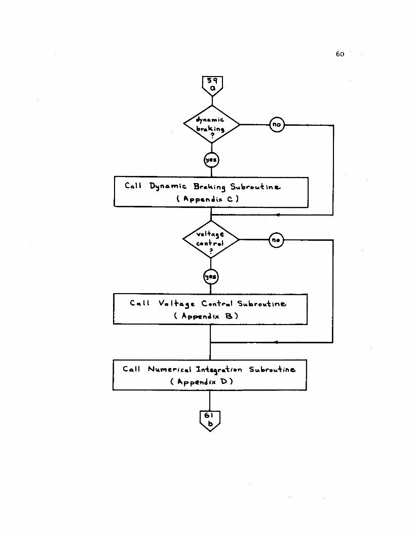
page 41. The flow chart is found as follows:
Main Program Appendix A
Voltage Damping Subroutine Appendix B
Dynamic Braking Subroutine Appendix C
Numerical Integration Subroutine Appendix D
The fourth order Runge Kutta method is used to obtain a numeri-
cal solution to the differential equation
for
r
Xli
X2i
X3 i
the ith
Xli
X2i
X 3i
E * i
generator where
= E.,
= g. = Air
= = i 1
= the required
integration
s E. i
X3 i
fi(Xlk'X2k)
E. to be held i period At
constant over the
43
(57)
and
fi(Xlk1 X2k) = 1 W.-X1iGi
M. i
c j=1
XliXljYijCos(Tij-X2i+X2j)
The Runge Kutta recursion formula is
where
X. (m+l )= , (m)+ 1 15.+1 R +1 S + 1 V.
6 i - 3
i 3 i 6
X. i
:
X2i
-
X 3i
(58)
(59)
(6o)
-
1 1
=
i
Ai,
Q.
R. i
Qli
Q2i
Q3 i
R1 i
R2i
R 3 i-
.
* E. i X3
fi(Xlk,X2k)
. * E. i
X3i+Q3i/2
fi(Xlk+Q1k1 X2k+Q2k) 2 2
At ,
At
V.
and
s31.
V1 i
V2i
V 3±
*
E. i X3i+R3i/2
fi(Xlk+R1k,X2k+R2k)
2 2
X +S 3i 3i
fi(Xlk+S1k,X2k+S2k)
44
(61 )
, (62)
At , (63)
At (64)
m = the number of the last computed period.
For all cases given, a step size, At, of 0.01 seconds is used.
The accuracy of these solutions have been verified by using a
step size of 0.005 seconds.
S1
S2i
. *
i E.
=
=
45
Reference Case
A disturbance may be introduced in the system by off-
setting the initial relative angles dl- d3 and 42- from
the steady -state equilibrium point for this system illustrated
in Figure 5. The undamped dynamic response with initial
relative angles of zero degrees is given in Figure 9. Damped
cases are to be given for this disturbance to demonstrate and
compare the damping methods.
Voltage Control Damping Cases
The damping equation for total voltage control is
É. = i Ei (52) i eLi + E Ri
and for local voltage control is
E. _ i Ei eLi
(53)
The required exciter output voltage, E xi
, may be found in terms
of E. by substitution of equation (55) into equation (56) to
give
( L R xi - l f i Ei+Ei } f i
Rfi Rfi
/1
K.
(65)
d3
R
ioo
80
46
First Overskoo4
20
to 20 30 40
¿a - S3 in De9rees
50
Figure 9. The Undamped Three -Generator Reference Case with Time Intervals Marked in Seconds on the Trajectory.
47
If the magnitude of the required exciter output voltage exceeds
five times its nominal value, a limit is imposed. The flow
chart for the voltage control subroutine is given in Appendix B.
A of ten is used for this system on both local and total
voltage control cases. It has been determined from other cases
not included in this thesis that damping increases as .11 is made
large although a limit is reached due to exciter saturation.
The dynamic response with total voltage control is given in
Figure 10 and the response with local voltage control is given
in Figure 11. It is noticed that these cases are quite similar
although somewhat better damping is obtained for total voltage
control.
For the purpose of comparison, the norm is defined as the
linear angular distance between the undamped steady -state
equilibrium point of Figure 9, and the maximum excursion of the
first overshoot. In both cases the norm is reduced by 59 per
cent from the undamped case.
The voltage response of each generator for both forms of
control is illustrated in Figure 12. The greatest difference
between the response with total and local voltage control occurs
at generator number two which has the least oscillation of all
three generators.
System responses not included in this thesis were also made
for initial relative angles of:
u
100
First Overshoot Final Sie^Jy -State. EVA; Is tar ¡um Point
"*-2.0
O 10 20
1.0
48
30 40
bt - 63 in De9rees
50
Figure 10. Total Voltage Control Applied to the Three - Generator Reference Case with Time Intervals Marked in Seconds on the Trajectory.
(}1 = 10 per-unit)
1
i
10
O
100
so
20
Overs koot Final Ste4Jy- Stoke. Equil;briurn Paint-
1.0
2.0
49
io ZO 30 40 So
Si - 63 in Degrees
Figure 11. Local Voltage Control Applied to the Three - Generator Reference Case with Time Intervals Marked in
Seconds on the Trajectory.
(}L = 10 per-unit)
C
`" 40 %.,o
..-Firsi 60
Figure 12. The Voltage Response of Each Generator with Local and Total Voltage Control Applied to the Three - Generator Reference Case.
(}I = 10 per -unit)
5i
To-tal Voltage Con-}rol
o.o I. O 2.0
I
Time. in Seconds
3.0 4.0
Gen. 2.
Ç Local Voltage Con +ro
0.0 LO 2.0
Tme in Seconds
3.0 4.0
Time in Seconds
0.0 1.0 2.0 3.0 4.0
52
á2 s3
40° 0°
40° 40°
80° 20°
Results of damping for these cases are comparative to the
damping for the case given.
Dynamic Braking Case
Control is directly exercised on each driving point con-
ductance in the three -generator model. For the application of
load resistors, AG. is added to G., and for load shedding AG.
is subtracted from Gi. The required size of AGi is given as
AG, = ñM,/E 2 (35)
Since the nominal value of E. and M, are identical for all
generators, AGi must also be identical. The coefficient
is chosen such that the application of OG. causes a step change
in Pi equal to ten per cent of the nominal W..
Thus
and
T = 0.1 W,/M. = 2.127
AG. = 0.179 for i = 1,2,3.
ól ó3
i
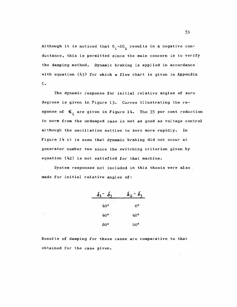
53
Although it is noticed that G. -AG. results in a negative con-
ductance, this is permitted since the main concern is to verify
the damping method. Dynamic braking is applied in accordance
with equation (43) for which a flow chart is given in Appendix
C.
The dynamic response for initial relative angles of zero
degrees is given in Figure 13. Curves illustrating the re-
sponse of Ei are given in Figure 14. The 35 per cent reduction
in norm from the undamped case is not as good as voltage control
although the oscillation settles to zero more rapidly. In
Figure 14 it is seen that dynamic braking did not occur at
generator number two since the switching criterion given by
equation (42) is not satisfied for that machine.
System responses not included in this thesis were also
made for initial relative angles of:
S1 S3 b2 - d3
40° 0°
40° 40°
80° 20°
Results of damping for these cases are comparative to that
obtained for the case given.
100
SO
54
First' Overshoot
o 10 20
Sa - S3
Final Steady- State Equil;brium Point
.5
30 4o
in De'rees
SO
Figure 13. Dynamic Braking Applied to the Three -Generator Reference Case with Time Intervals in Seconds Marked on the Trajectory.
(X = 2.127 per -unit)
' C
1\
55
Time In Seconds
Time in Seconds
Gen. 3
Figure 14. Response of E. with Dynamic Braking Applied to the Three -Generator Reference Case. For Interpretation of Discontinuities see Figure 6.
(N= 2.127 per -unit)
o
56
Prime Mover Control
A case is not given for the control of W, to introduce i
damping by
YM. i0i Ei (31)
since present governor and turbine systems cannot follow the
equation for most oscillation frequencies. This equation has
been developed, however, in anticipation of improvements in the
prime mover response.
.
W. _ i
-
57
BIBLIOGRAPHY
1. Benson, Arden R. Control of generation in the U. S.
Columbia River power system. 4th ed. Portland, U. S.
Bonneville Power Administration, 1966. 41 numb. leaves. (Duplicated)
2. Blythe, A. L. and R. M. Shier. Field tests of dynamic stability using a stabilizing signal and computer program verification. IEEE Power Apparatus and Systems 87:315- 322. 1968.
3. El- Abiad, Ahmed H. and K.Nagappan. Transient stability regions of multimachine power systems. IEEE Trans- actions on Power Apparatus and Systems 85:169 -179. 1966.
4. Ellis, H. M. et al. Dynamic stability of the Peace River transmission system. IEEE Transactions on Power Apparatus and Systems 85:586 -600. 1966.
5. Fringe generation damps tie -line oscillation. Electrical World 165:48 -49, 84 -85. Jan. 10, 1966.
6. Gless, G. E. The direct method of Liapunov applied to transient power system stability. IEEE Transactions on Power Apparatus and Systems 85:159 -168. 1966.
Jones, G. A. Transient stability of a synchronous generator under conditions of bang -bang excitation sched- uling. IEEE Transactions on Power Apparatus and Systems 84:114 -121. 1965.
8. Kimbark, E. W. Improvement of system stability by switched series capacitors. IEEE Transactions on Power Apparatus and Systems 85:180 -188. 1966.
9. Kimbark, E. W. Power system stability. Vol. 1. New York, John Wiley, 1956. 322 p.
10. Mittelstadt, W. A. Four methods of power system damping. IEEE Transactions on Power Apparatus and Systems. Vol. 87. May, 1968. (In press)
11. Schleif, F. R., G. E. Martin and R. R. Angell. Damping of
system oscillations with a hydrogenerating unit. IEEE Transactions on Power Apparatus and Systems 86:438 -442. 1967.
7.
58
12. Schleif, F. R. and J. Hi White. Damping for the Northwest Southwest tie -line oscillations - an analog study. IEEE Transactions on Power Apparatus and Systems 85:1239 -1247. 1966.
13. Smith, O.J.M. Optimal transient removal in a power system. IEEE Transactions on Power Apparatus and Systems 84:361 -374. 1965.
14. Stevenson, William D., Jr. Elements of power system analysis. 2d ed. New York, McGraw Hill, 1962. 388 p.
15. U. S. Dept. of the Interior. Bonneville Power Administra- tion. Pacific Northwest- Southwest intertie. [Portland], n.d. 14 p.
16. Van Vranken, W. P. Improving hydrogenerator stability with static excitation. Allis- Chalmers Engineering Review 32(3):20 -22. 1967.
17. Yu, Y. and K. Vongsuriya. Nonlinear power system stability study by Liapunov function and Zubov's method. IEEE Transactions on Power Apparatus and Systems 86:1480 -1485. 1967.
-
A P P E N D I C E S
Appendix A. The Main Program Flow Chart for Power System Simulation.
( START)
READ BASIC SYSTEM DATA N number of genera generators Yj transfer odnntttonce* Ç. transfer admittance } tonca ongles Gi Jrtv'n3 point conductances Ef generator voltages Wi generator powers Mi inertia constants
59
(al
READ CASE. DETAILS A+ inte'rotion step sise. Tm.x maximum solution time. di in' {ial generator angles A sly braking coefficient ,u voltage control coeÇftctnt Lri generator