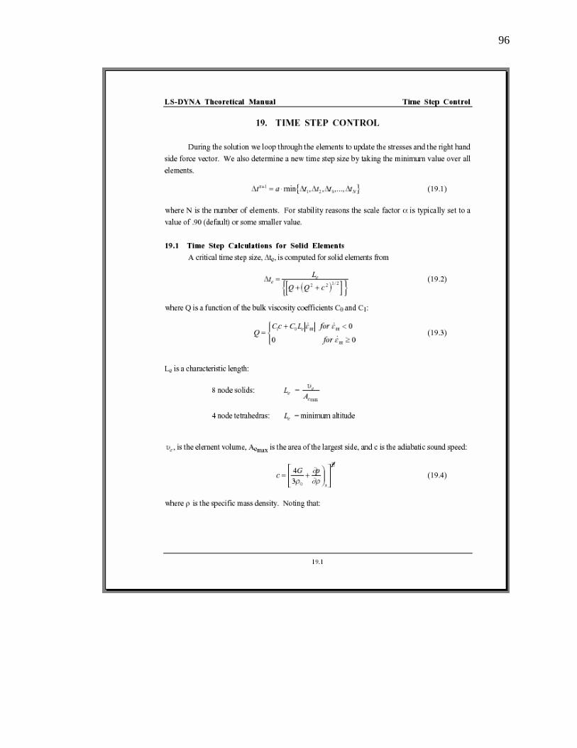
A Method to Evaluate and Predict the Performance of Baseball Bats Using Finite Elements TIMOTHY J. MUSTONE B.S.M.E. UNIVERSITY OF MASSACHUSETTS LOWELL (1996) SUBMITTED IN PARTIAL FULFILLMENT OF THE REQUIREMENTS FOR THE DEGREE OF MASTER OF SCIENCE DEPARTMENT OF MECHANICAL ENGINEERING UNIVERSITY OF MASSACHUSETTS LOWELL Signature of Author:__________________________________________Date:________________________________ Signature of Thesis Supervisor: __________________________________________________________ Signatures of Thesis Committee Members: __________________________________________________________ __________________________________________________________
Transcript
A Method to Evaluate and Predict the Performance of Baseball Bats Using Finite Elements
TIMOTHY J. MUSTONE B.S.M.E. UNIVERSITY OF MASSACHUSETTS LOWELL (1996)
SUBMITTED IN PARTIAL FULFILLMENT OF THE REQUIREMENTS FOR THE DEGREE OF MASTER OF SCIENCE
DEPARTMENT OF MECHANICAL ENGINEERING UNIVERSITY OF MASSACHUSETTS LOWELL
Signature of Author:__________________________________________Date:________________________________ Signature of Thesis Supervisor: __________________________________________________________ Signatures of Thesis Committee Members: __________________________________________________________
A Method to Evaluate and Predict the Performance of Baseball Bats Using Finite Elements
TIMOTHY J. MUSTONE B.S.M.E. UNIVERSITY OF MASSACHUSETTS LOWELL (1996)
SUBMITTED IN PARTIAL FULFILLMENT OF THE REQUIREMENTS FOR THE DEGREE OF MASTER OF SCIENCE
DEPARTMENT OF MECHANICAL ENGINEERING UNIVERSITY OF MASSACHUSETTS LOWELL
2003
Thesis Supervisor: Dr. James A. Sherwood Professor, Department of Mechanical Engineering
iii
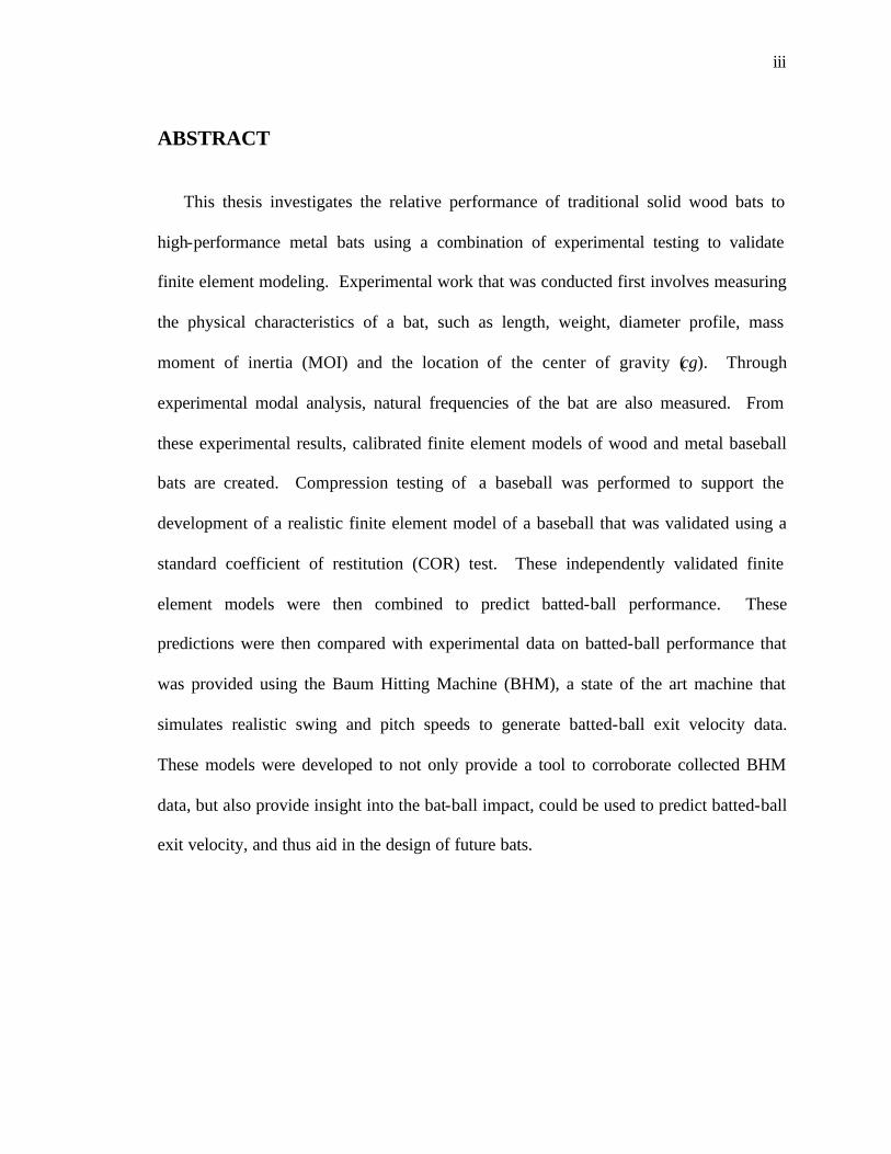
ABSTRACT
This thesis investigates the relative performance of traditional solid wood bats to
high-performance metal bats using a combination of experimental testing to validate
finite element modeling. Experimental work that was conducted first involves measuring
the physical characteristics of a bat, such as length, weight, diameter profile, mass
moment of inertia (MOI) and the location of the center of gravity (cg). Through
experimental modal analysis, natural frequencies of the bat are also measured. From
these experimental results, calibrated finite element models of wood and metal baseball
bats are created. Compression testing of a baseball was performed to support the
development of a realistic finite element model of a baseball that was validated using a
standard coefficient of restitution (COR) test. These independently validated finite
element models were then combined to predict batted-ball performance. These
predictions were then compared with experimental data on batted-ball performance that
was provided using the Baum Hitting Machine (BHM), a state of the art machine that
simulates realistic swing and pitch speeds to generate batted-ball exit velocity data.
These models were developed to not only provide a tool to corroborate collected BHM
data, but also provide insight into the bat-ball impact, could be used to predict batted-ball
exit velocity, and thus aid in the design of future bats.
iv
ACKNOWLEDGMENTS
Major League Baseball and Rawlings Sporting Goods, Inc. for providing the grant to establish the UMass Lowell Baseball Research Center. The National Collegiate Athletic Association, for using the UMass Lowell Baseball Research Center as an official test center. Representatives from baseball bat manufacturers: Worth, Rawlings, Hoosier Bat Company, Easton Sports and Hillerich and Bradsby (H&B) for providing insight into baseball bat design and testing methodologies. Past and present students who have worked in the UMass Lowell Baseball Research Center, for continuing what was started and making improvements along the way. Dr. Peter Avitabile and Dr. Struan Robertson, for taking the time to be a part of my thesis committee. To all my friends who have helped me, by continually asking how the thesis is going. Larry Fallon of Sports Engineering, for introducing baseball bat testing to UMass Lowell and for being a great friend. Dr. Jim Sherwood, for being not only my thesis advisor, but also a friend and someone whom I’ve learned a great deal from. My parents, John and Muriel Mustone, for always pushing me to do my best; my brothers Jamie and Andy and my sister Missy, for all those whiffle ball games in the back yard. My daughter Quinn, for making me laugh with those baby giggles when I needed a break from typing; and my wife Mea, for your unconditional love and support - I couldn’t have done any of it without you.
v
TABLE OF CONTENTS
ABSTRACT....................................................................................................................... iii ACKNOWLEDGMENTS ..................................................................................................iv TABLE OF CONTENTS.....................................................................................................v LIST OF TABLES ............................................................................................................ vii LIST OF FIGURES ......................................................................................................... viii 1 INTRODUCTION ...................................................................................................... 1
1.1 NCAA Addresses Bat Performance .................................................................... 1 1.2 Scope................................................................................................................... 5
2 BACKGROUND ........................................................................................................ 6 2.1 Introduction to Engineering Concepts relating to Baseball ................................ 6
2.1.1 Coefficient of Restitution............................................................................ 6 2.1.2 Mass Moment of Inertia and Parallel Axis Theorem.................................. 9 2.1.3 Center of Percussion and Sweet Spot ....................................................... 11
2.2 Wood vs. Metal................................................................................................. 12 2.2.1 The Bat-Ball Collision and Energy Transfer ............................................ 12
2.3 Performance Statistics of Wood vs Metal......................................................... 20 2.3.1 Thurston’s Cape Cod League Study ......................................................... 20 2.3.2 Sports Engineering Field Performance Study........................................... 21
2.4 Crisco’s Final Report to the NCAA.................................................................. 22 2.4.1 Relationship between Reaction Time and Injuries due to the Batted Ball 23 2.4.2 Predicting Ball Performance ..................................................................... 24 2.4.3 Predicting Bat Performance ...................................................................... 28 2.4.4 Effects of Bat Mass and Inertia................................................................. 33
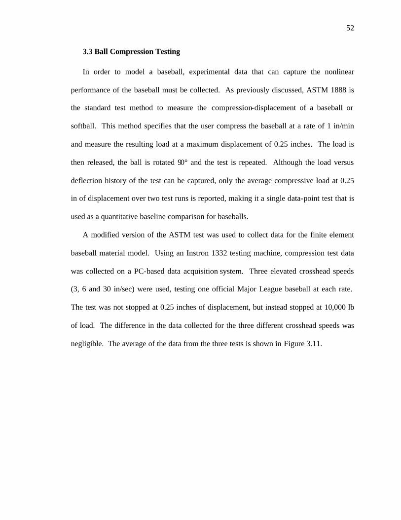
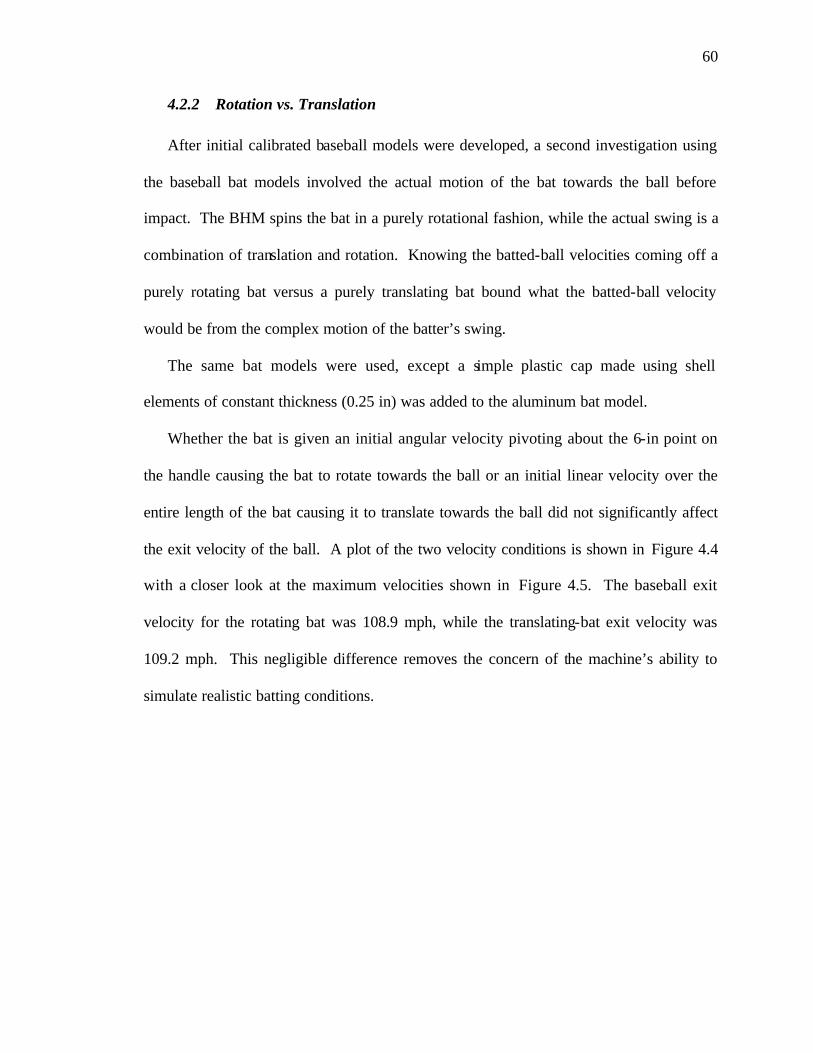
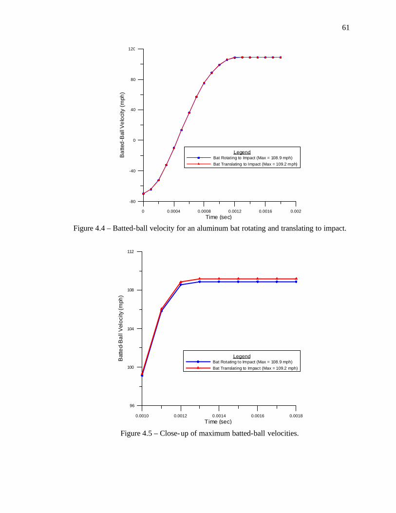
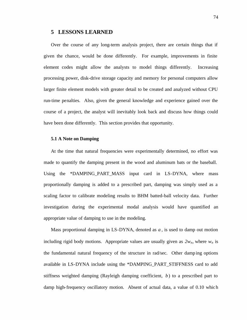
4.1 Analysis Tools Used ......................................................................................... 54 4.2 Early BHM Models ........................................................................................... 55
4.2.1 The 290° Swing vs. The 0° Swing ............................................................ 58 4.2.2 Rotation vs. Translation............................................................................ 60
4.3 Modeling Calibration........................................................................................ 62 4.3.1 Calibrating the Baseball Model................................................................. 63 4.3.2 Calibrated Ball Results.............................................................................. 64 4.3.3 Calibrating the Baseball Bat Models ........................................................ 67 4.3.4 Calibrated Baseball Bat Results ................................................................ 69
5 LESSONS LEARNED.............................................................................................. 74 5.1 A Note on Damping .......................................................................................... 74
vi
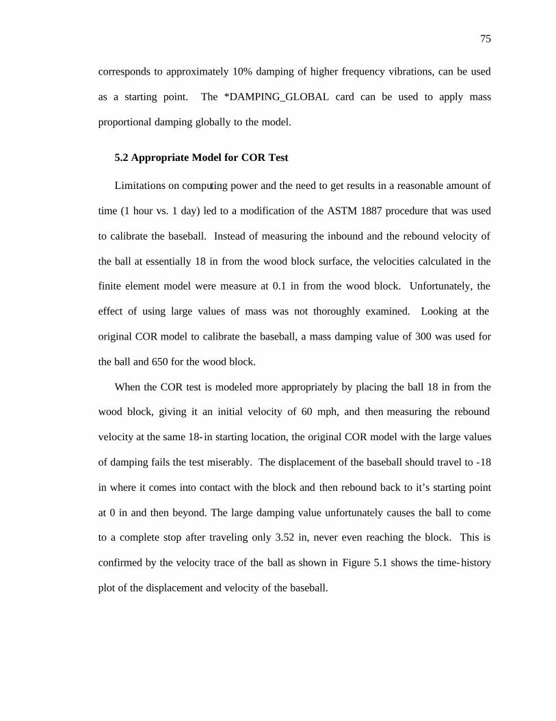
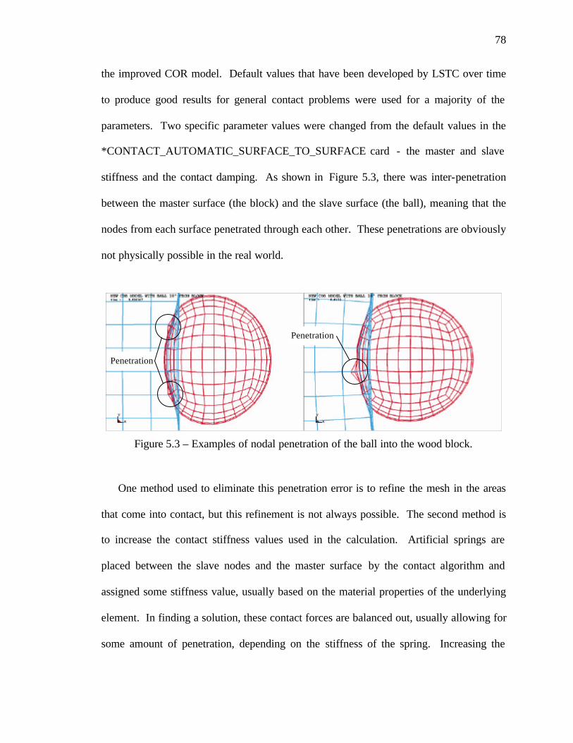
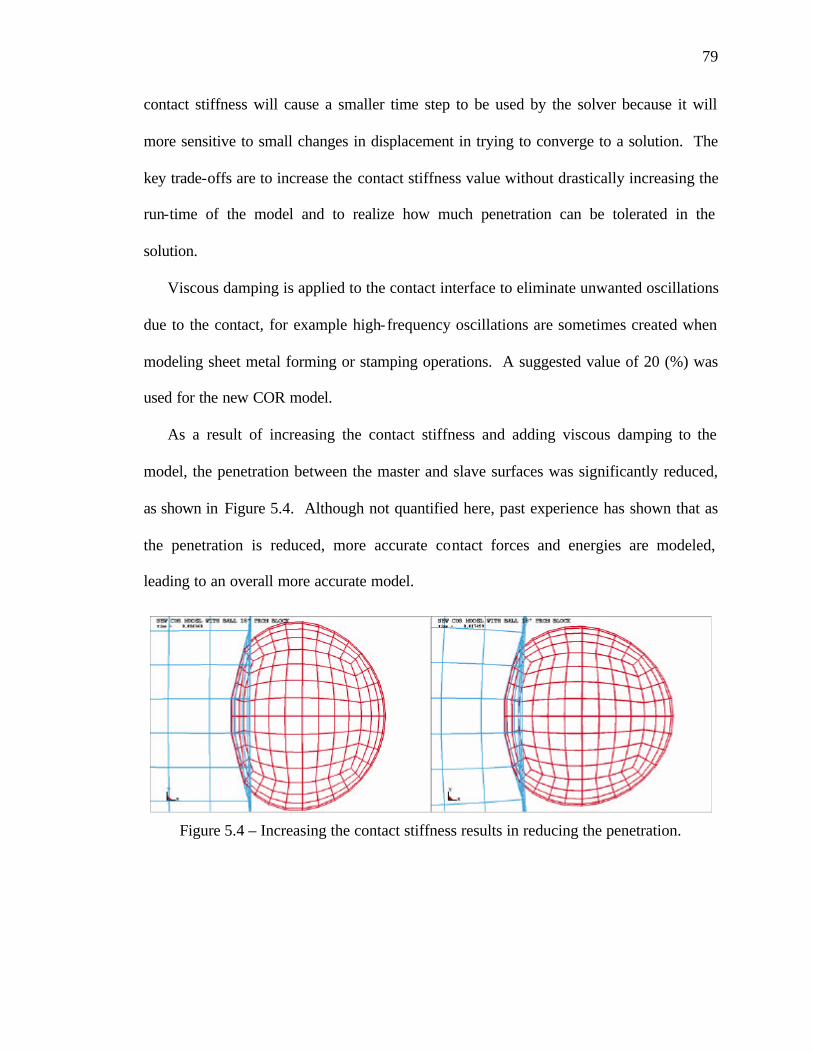
5.2 Appropriate Model for COR Test ..................................................................... 75 5.3 Modifying contact analysis parameters............................................................. 77 5.4 Corrected Aluminum Bat Model ...................................................................... 80
5.4.1 Wall Thickness and Nodal Reference Plane for Shell Elements .............. 80 5.4.2 MOI Calibration........................................................................................ 83
5.5 Updated Model Comparison............................................................................. 83 6 CONCLUSIONS AND recommendations ............................................................... 90
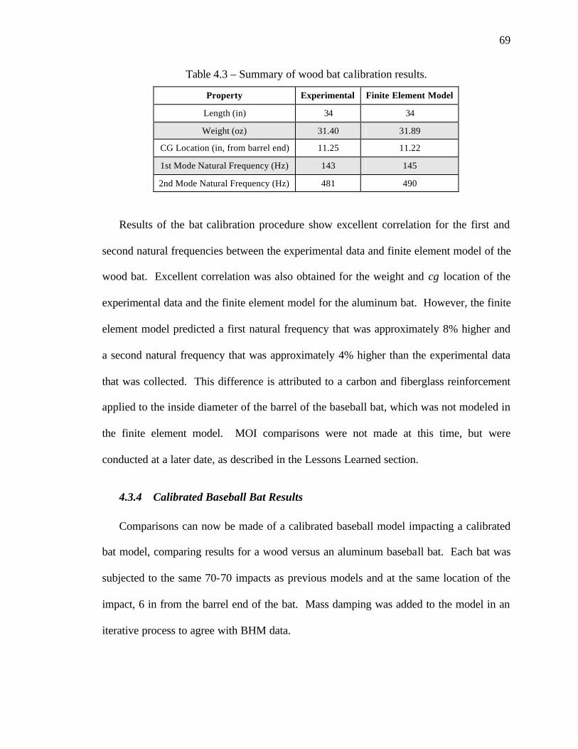
Table 2.1 – Comparison of player's statistics (1997 data). ............................................... 20 Table 2.2 – Statistical summary of field performance data. ............................................. 22 Table 2.3 – Ball compression test results.......................................................................... 28 Table 2.4 – Results of parametric study. ........................................................................... 36 Table 3.1 – Experimental frequency results...................................................................... 51 Table 4.1 – Summary of material properties used for initial modeling. ........................... 57 Table 4.2 – Summary of aluminum bat calibration results. .............................................. 68 Table 4.3 – Summary of wood bat calibration results. ..................................................... 69 Table 5.1 – Summary of updated aluminum bat calibration results. ................................ 83 Table 5.2 – Summary of wood bat calibration results. ..................................................... 83 Table 5.3 – Summary of batted-ball velocity comparison. ............................................... 85
viii
LIST OF FIGURES
Figure 2.1 - Two bodies in motion, before (top), during (middle) and after (bottom) a collision. ...................................................................................................................... 7
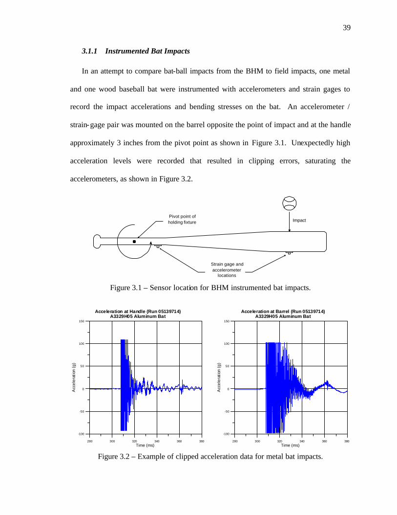
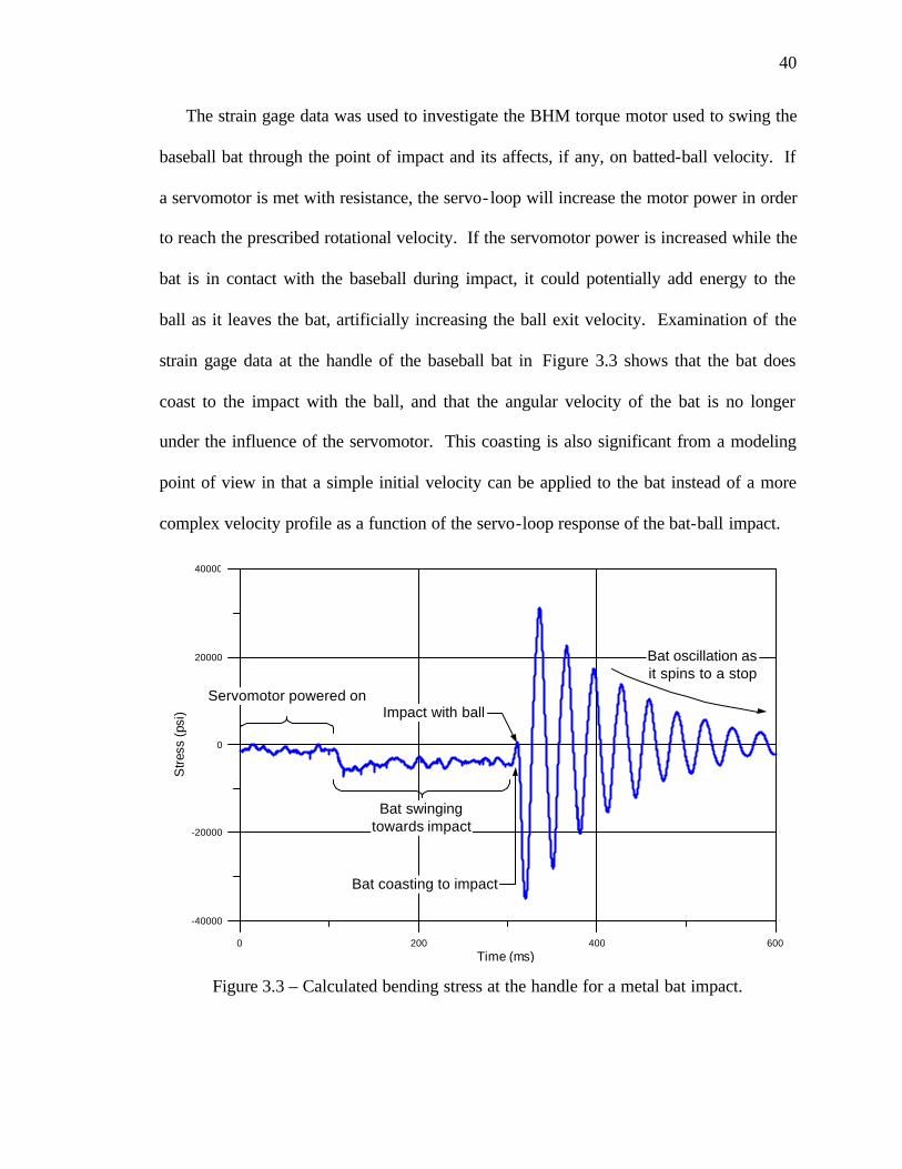
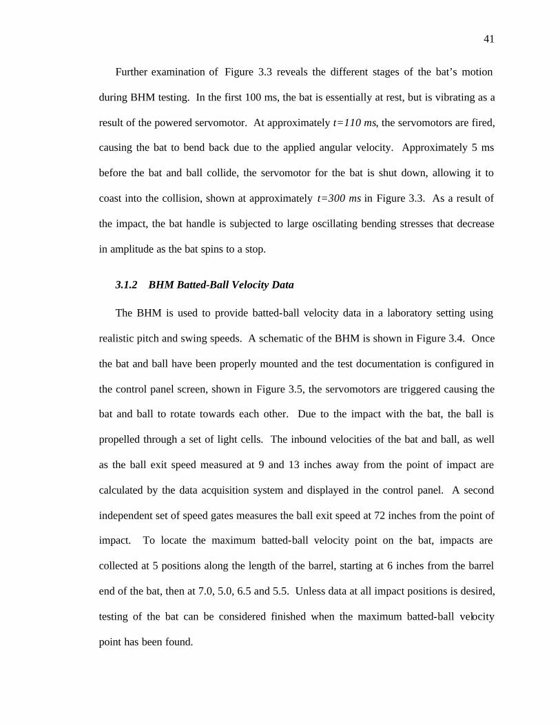
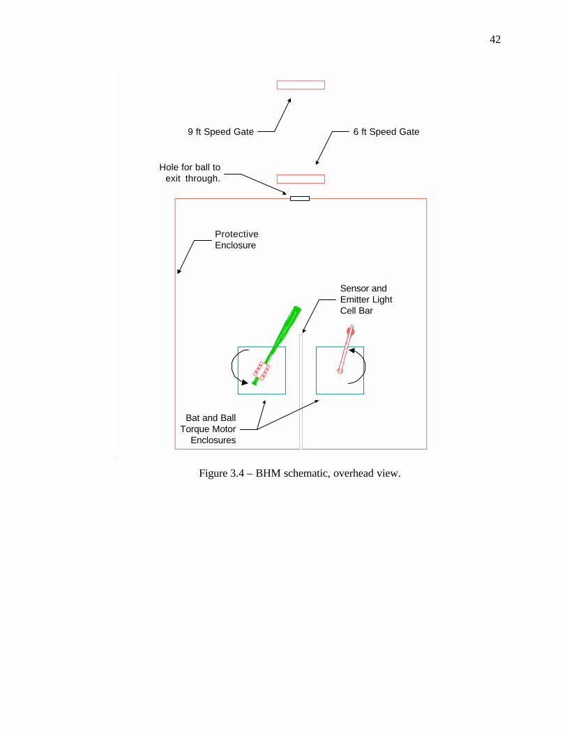
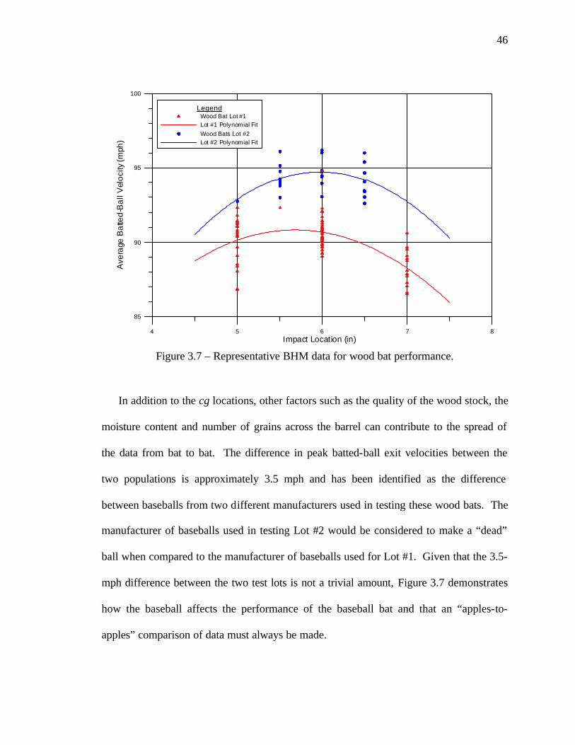
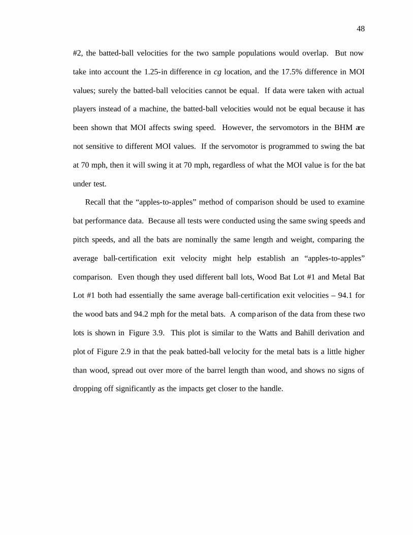
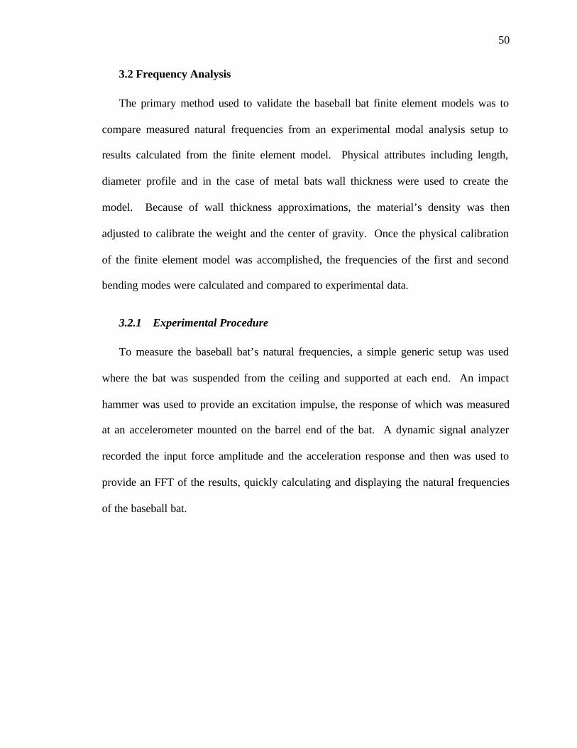
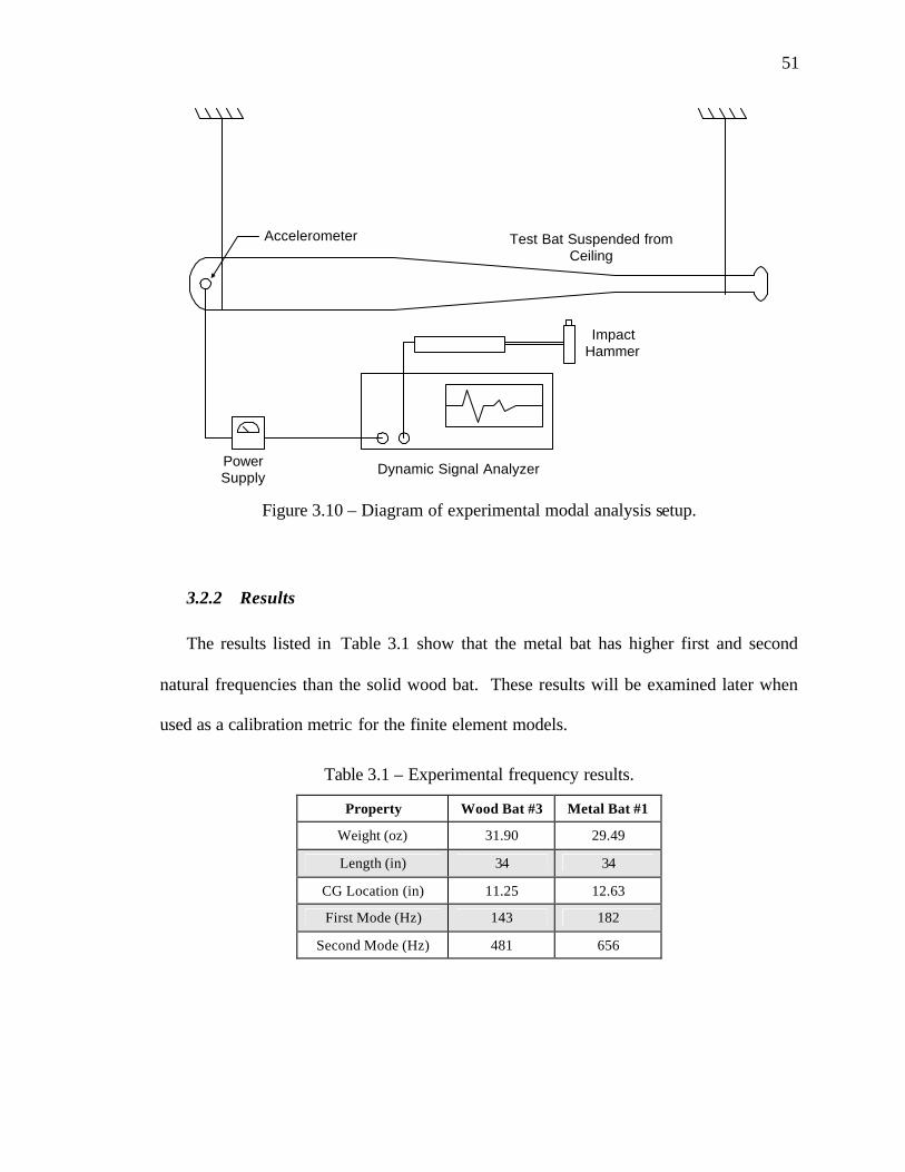
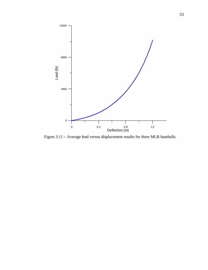
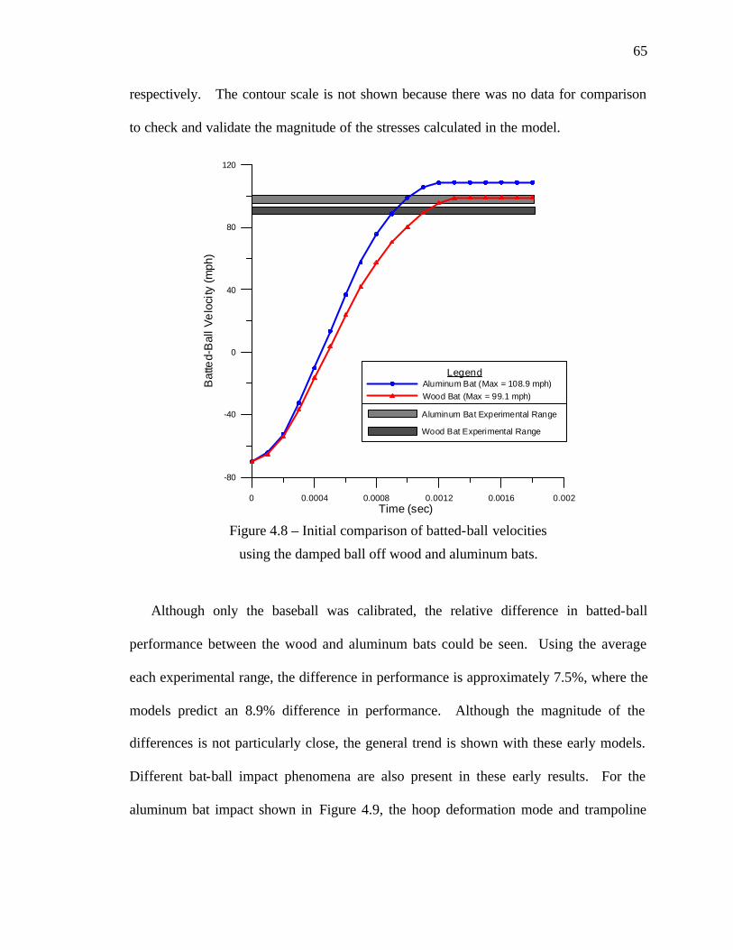
Figure 2.2 – Baseball bat MOI terminology. .................................................................... 10 Figure 2.3 – Comparing typical MOI values for wood and metal bats............................. 11 Figure 2.4 – An example of the bending deformation...................................................... 13 Figure 2.5 – Bat-ball collision showing local trampoline ................................................. 14 Figure 2.6 – Example of a hollow metal bat with a composite barrel-reinforcement. ..... 15 Figure 2.7 – Motion of the swinging bat........................................................................... 16 Figure 2.8 – Variables denoted in swing equations. ......................................................... 17 Figure 2.9 – Plot demonstrating Equation 2.17. ............................................................... 19 Figure 2.10 – Cross-section of a baseball. ........................................................................ 27 Figure 2.11 – An example of the ASTM ball compression test and resulting data. ......... 27 Figure 2.12 – Schematic of Brandt test setup. .................................................................. 29 Figure 2.13 – Assorted views of the BHM. ...................................................................... 31 Figure 3.1 – Sensor location for BHM instrumented bat impacts. ................................... 39 Figure 3.2 – Example of clipped acceleration data for metal bat impacts. ....................... 39 Figure 3.3 – Calculated bending stress at the handle for a metal bat impact.................... 40 Figure 3.4 – BHM schematic, overhead view. .................................................................. 42 Figure 3.5 – Sample BHM data sheet. .............................................................................. 43 Figure 3.6 – Example of variability within and between ball lots (valid hits only). ........ 44 Figure 3.7 – Representative BHM data for wood bat performance. ................................. 46 Figure 3.8– Representative BHM data for metal bat performance. .................................. 47 Figure 3.9 – Comparison of wood and metal bat BHM data. ........................................... 49 Figure 3.10 – Diagram of experimental modal analysis setup.......................................... 51 Figure 3.11 – Average load versus displacement results for three MLB baseballs. ......... 53 Figure 4.1 – Initial bat-ball impact models for the ........................................................... 56 Figure 4.2 – 290° swing model (left) and 0° swing model (right). ................................... 58 Figure 4.3 – Results of BHM swing study for 290° and 0° swings. ................................. 59 Figure 4.4 – Batted-ball velocity for an aluminum bat rotating and translating to impact.
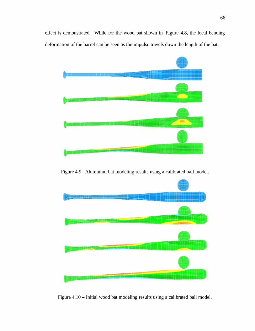
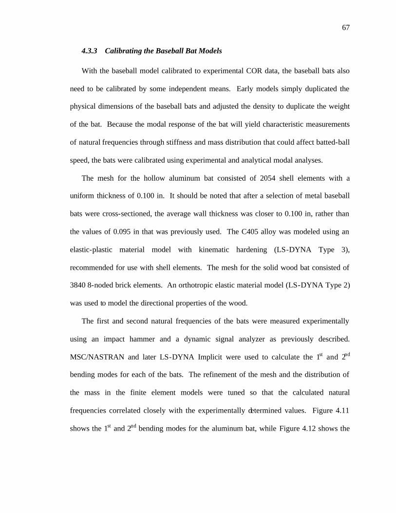
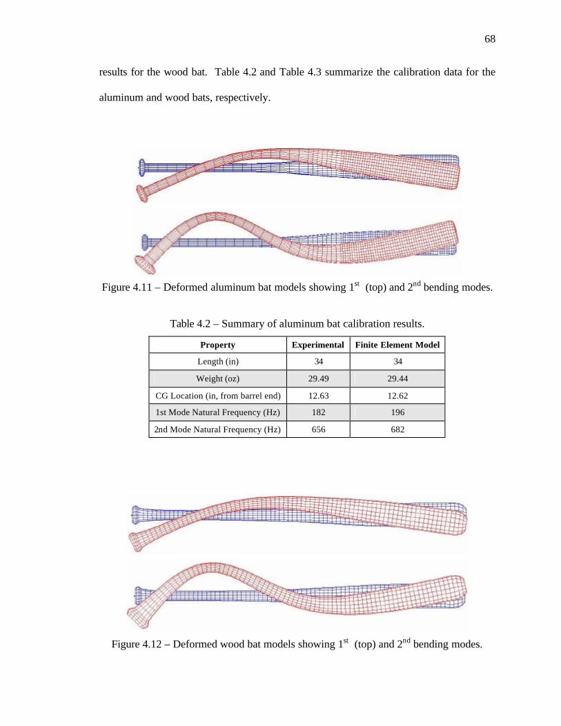
................................................................................................................................... 61 Figure 4.5 – Close-up of maximum batted-ball velocities................................................ 61 Figure 4.6 – New finite element meshes for the aluminum bat (top) ............................... 62 Figure 4.7 – Sequence of ball deformation during contact with flat surface. ................... 64 Figure 4.8 – Initial comparison of batted-ball velocities .................................................. 65 Figure 4.9 –Aluminum bat modeling results using a calibrated ball model. .................... 66 Figure 4.10 – Initial wood bat modeling results using a calibrated ball model. ............... 66 Figure 4.11 – Deformed aluminum bat models showing 1st (top) and 2nd bending modes.
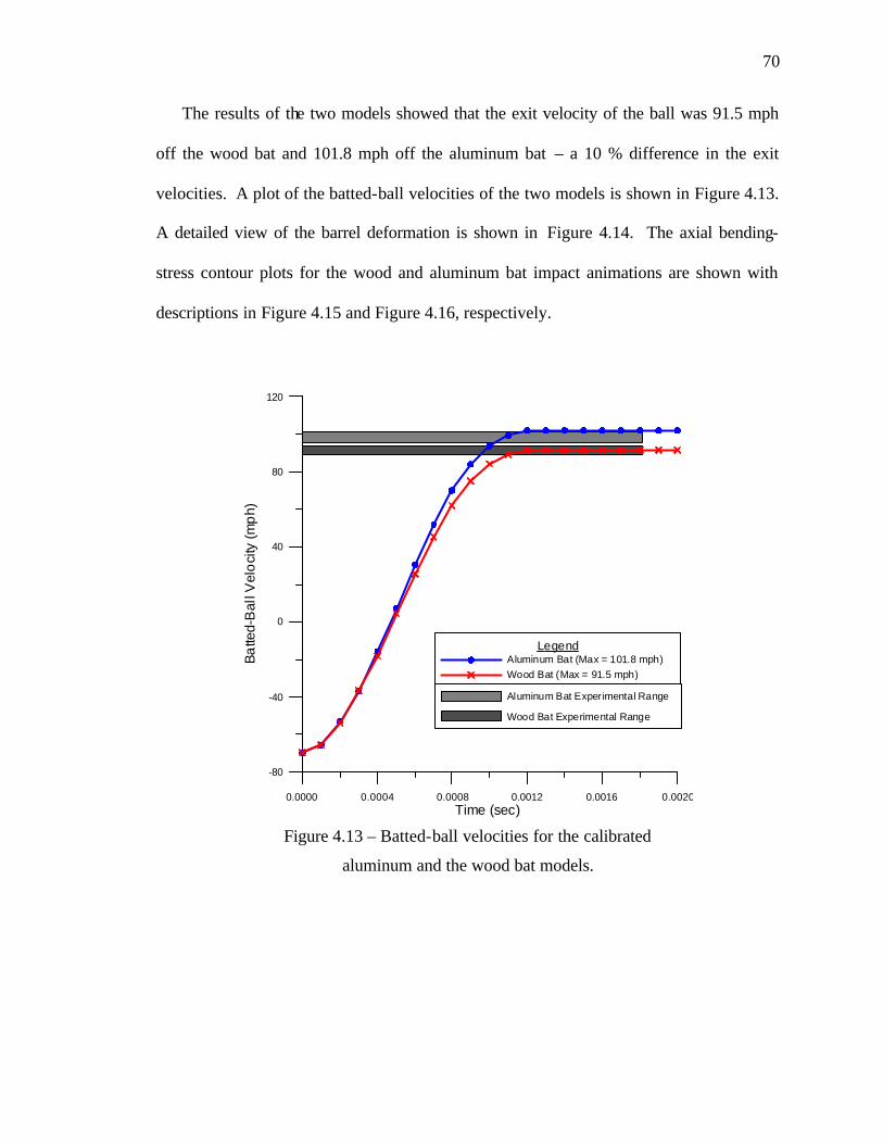
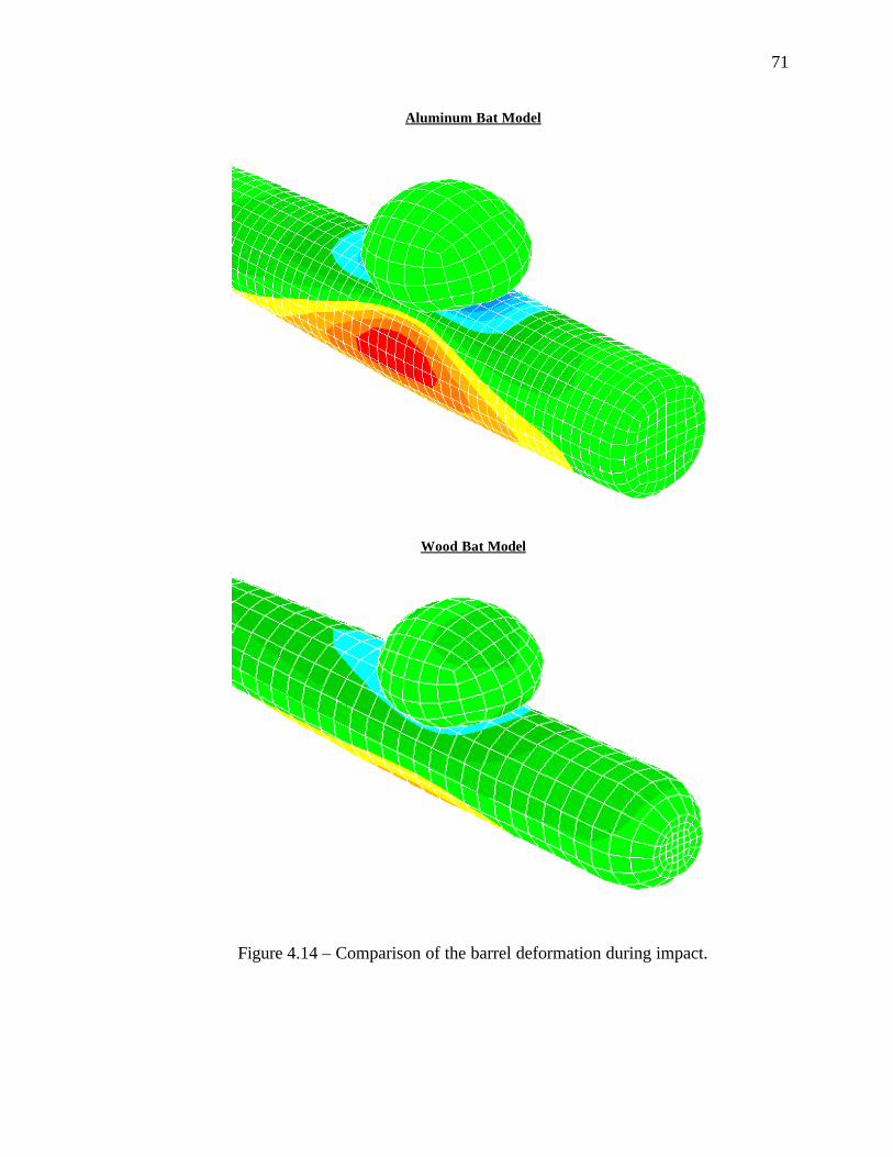
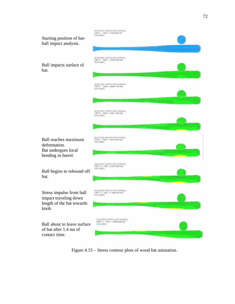
................................................................................................................................... 68 Figure 4.12 – Deformed wood bat models showing 1st (top) and 2nd bending modes..... 68 Figure 4.13 – Batted-ball velocities for the calibrated...................................................... 70 Figure 4.14 – Comparison of the barrel deformation during impact. ............................... 71 Figure 4.15 – Stress contour plots of wood bat animation. .............................................. 72 Figure 4.16 – Stress contour plots of aluminum bat animation. ....................................... 73
ix
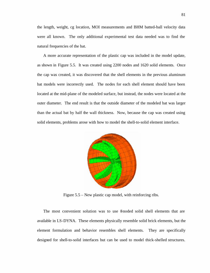
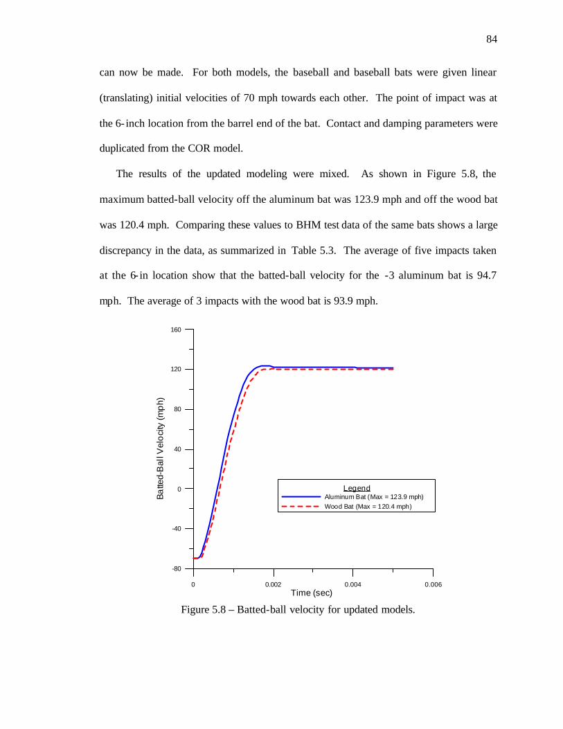
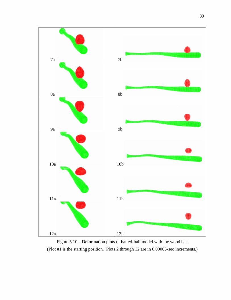
Figure 5.1 – Displacement and velocity of original baseball COR model. ...................... 76 Figure 5.2 – Improved COR model results for baseball displacement and velocity. ....... 77 Figure 5.3 – Examples of nodal penetration of the ball into the wood block. .................. 78 Figure 5.4 – Increasing the contact stiffness results in reducing the penetration. ............ 79 Figure 5.5 – New plastic cap model, with reinforcing ribs............................................... 81 Figure 5.6 – Sectioned view showing interface with cap. ................................................ 82 Figure 5.7 – Updated aluminum bat model. ..................................................................... 82 Figure 5.8 – Batted-ball velocity for updated models....................................................... 84 Figure 5.9 – Time-history plot of the batted-ball displacement........................................ 86 Figure 5.10 – Deformation plots of batted-ball model with the wood bat........................ 89
1
1 INTRODUCTION
1.1 NCAA Addresses Bat Performance
In 1974, the National Collegiate Athletic Association (NCAA) permitted the use of
aluminum bats in collegiate baseball games under its jurisdiction. The initial purpose for
this change from traditional solid wood to aluminum was to reduce operating costs due to
broken bats. The original aluminum bats performed similar to wood, with the exception
that the aluminum bats did not break. As aluminum alloy performance and competition
among the sporting goods manufacturers increased, so did the performance of the
aluminum bats resulting in a new generation of high-performance baseball bats being
developed. These new bats used the latest advances in technology, including new metal
alloys, damping materials and sensors and barrel reinforcements such as air bladders and
composite materials.
Baseball bat performance comes down to a simple physics problem: the higher the
initial exit velocity of a batted ball, the farther the ball will travel. As more technological
advances were added to metal bats, the performance gap versus traditional wood bats
widened. This increasing performance has upset the balance between the offense and
defense of the game, compromising the integrity of the game itself.
At the 1995 College World Series, a record 48 home runs were hit during the 16-
game series, breaking the previous mark of 29. During the 1998 College World Series,
64 home runs were hit setting another record. The score of the 1998 final championship
game was 21 to 14, a typical football score, not a baseball score. Clearly one or more
factors were causing this increase in offense.
2
A side effect of the increasing bat performance is the potential danger to pitchers who
might be unable to defend themselves against a line drive hit by these new bats. A
batted-ball traveling at an elevated velocity could sometimes reach the pitcher faster than
it takes for the pitcher to defend himself. Although there has been no definitive study,
media outlets most often report injuries to pitchers from Little League, high school and
college caused by the use of these high-performance baseball bats, in comparison to
reporting injuries caused by wood bats.
Amherst College head baseball coach Bill Thurston conducted a preliminary study in
1997 that compared the hitting statistics of players who participated in NCAA Division I
baseball with aluminum bats and then played in the Cape Cod League the following
summer.1 The Cape Cod League is one of a handful of summer leagues that uses
traditional wood bats. A total of 88 college players were considered in the statistical
study. To be eligible for the study, a player had to have a minimum of 70 at-bats in the
Cape Cod League. In summary, Thurston found that the average batting average for all
the players decreased by 100 points, the number of home runs per-at-bat decreased by
65% and the number of strikeouts per-at-bat increased by 41%, while the number of
walks remained the same. It became evident how much the aluminum bat can influence
the offensive aspects of the game.
Major League Baseball (MLB) became involved in the debate because a considerable
number of its players are drafted from the college ranks. After playing with an aluminum
bat for most of their baseball career, with the exception of playing in a summer league
that exclusively uses wood bats, rookie players have a difficult time adjusting to hitting
the ball with a wood bat. It takes on average two years for a player to learn how to hit
3
with a wood bat. Because of the inherent difference between playing with a wood bat and
playing with a metal bat, talent scouts from MLB organizations have difficulty evaluating
a potential draft-pick’s offensive skills. They have to translate the skill that a player has
hitting with a metal bat to how that player will do when he uses a wood bat.
To better understand the bat performance issue, consider the timeline of events
regarding how the NCAA has addressed bat performance as discussed in the February
1999 edition of the NCAA News.2 The first step that the NCAA took to curb the new
generation of aluminum bats was for the 1989 season. It restricted the weight of a metal
bat by setting a limit on how light they could be stating that the numerical difference
between the length and weight of a bat could not exceed five units, that is, a 34-in bat
could weigh no less than 29 oz. After the 1994 NCAA baseball season, the NCAA
Baseball Rules Committee met with the metal-bat manufacturers to discuss performance
issues. It was agreed tha t the performance level would not increase and that the Brandt
test, developed by New York University physics professor R. A. Brandt, PhD, would be
used to measure the performance. The Brandt test, to be discussed later, is a test
designed to measure the batted-ball performance of slow-pitch softball bats. Over the
next three seasons, the NCAA suspected that bat performance had increased. However,
the manufacturers reported that bat performance had not increased per the Brandt test. In
the fall of 1997, the NCAA was made aware of a letter written by Brandt, stating that his
test, adopted by the manufacturers as the bat performance testing standard, does not
accurately measure bat performance for baseball. As a result, Dr. J. J. Trey Crisco of the
National Institute for Sport Science and Safety (NISSS) and Brown University was
contracted to investigate several aspects of bat and ball performance, including the
4
evaluation of current testing methods. The findings of his report, to be discussed later,
only added to the controversy.
In July 1998, the NCAA Baseball Rules Committee held a “bat summit” where
invited researchers and guests were gathered to discuss bat-ball performance issues. The
guests in attendance included NCAA representatives, National Federation of High School
(NFHS) Baseball Rules Committee members and several bat manufacturers. A former
baseball bat design consultant for Hillerich & Bradsby (H&B, makers of the Louisville
TPX brand of metal bats and Louisville Slugger brand of wood bats) alleged that the
manufacturers of metal bats had misled and deceived the NCAA about bat performance
and testing standards. After assessing the gathered information, the rules committee
decided to develop new standards to limit the performance of metal bats, making them
perform more like wood bats. In developing the new standards, three requirements were
mandated: to minimize risk, to maintain a balance between offense and defense and to
preserve the integrity of the game. The three new recommended standards were:
1. Changing the weight to length unit difference from -5 (with the grip) to -3 (without the grip), meaning that a 34- in bat can weigh no less than 31 oz
2. Reducing the barrel diameter from 2 3/4 to 2 5/8 in 3. Limiting the batted-ball velocity to 94 mph, given a 70-mph pitch speed and a
70-mph swing speed at the point of impact, designated as the 6 in from the barrel-end of the bat
In a press release issued by the NCAA3, the Baseball Rules Committee felt that these
changes were necessary to make the game safer for all players and to improve
competitive balance between offensive and defensive aspects of the game. The
committee also felt that technological innovations, rather than player's skills, were
impacting the outcome of the games, threatening the integrity of college baseball.
5
1.2 Scope
This thesis will examine several aspects of baseball bat performance, which could
also be translated to softball bats, and primarily looks at the relative performance of high-
performance metal bats to traditional solid wood bats. Experimental work pertaining to
bat performance involves first measuring the physical characteristics of a bat, such as
length, weight, diameter profile, moment of inertia (MOI) and the location of the center
of gravity (cg). Through modal analysis, the natural dynamic characteristics of the bat
are measured. From these experimental results, calibrated finite element models of wood
and metal baseball bats are created. Compression testing of a baseball was performed to
support the development of a realistic finite element model of a baseball. This baseball
model was then used to examine the batted-ball performance of wood and metal baseball
bats using finite element modeling techniques. Experimental data on batted-ball
performance was provided using the Baum Hitting Machine (BHM), a state of the art
machine that simulates realistic swing and pitch speeds to generate batted-ball exit
velocity data. The finite element models not only provide a tool to corroborate collected
BHM data, but also provide insight into the bat-ball impact, could be used to predict
batted-ball exit velocity, and thus aid in the design of future bats.
6
2 BACKGROUND
2.1 Introduction to Engineering Concepts relating to Baseball
Before discussing the performance of baseballs and baseball bats, a few engineering
concepts are presented. The coefficient of restitution (COR) is used to quantify the
elasticity or “liveliness” of the baseball. The moment of inertia (MOI) of the baseball bat
has an important effect on the swing speed that a batter can generate. This swing speed
in turn has an effect on the batted-ball velocity. Several other concepts, like the center of
gravity or balance point of the baseball bat, the center of percussion and the “sweet spot”
also play a role in baseball bat performance. The following is a brief description of each
concept.
2.1.1 Coefficient of Restitution
The most accepted means of quantifying ball performance is to measure the COR of
the baseball as it strikes a stationary object, usually a thick white ash board rigidly
mounted to a wall. The COR is a measure of how elastic or inelastic two bodies are
when they come into contact with each other and must be measured experimentally. The
following is a brief derivation of the COR, as defined by Riley and Sturges.4 Consider
two bodies, A and B that are positioned on the same path as shown in Figure 2.1. Bodies
A and B are given initial velocities, vAi and vBi, respectively.
7
A BvAi vBi
A B
A BvAf
vBf
mAmB
Figure 2.1 - Two bodies in motion, before (top), during (middle) and after (bottom) a
collision.
It is assumed that during the brief interval that the two bodies are in contact, the
velocity of one or both of the bodies in motion may change and the positions of the
bodies do not change significantly. Also, non- impulsive forces and the friction forces
between the two bodies may be neglected.
Given the masses of each body, mA and mB, the total momentum for the two bodies
before (i) and after (f) the collision is conserved:
BfBAfABiBAiA vmvmvmvm +=+ Equation 2.1
Now consider the impulse forces acting on the individual bodies while the bodies are
deforming during and after the collision. When the two bodies are in contact, the
momentum equation gives
cA
t
tdAiA vmdtFvm
c
i
=− ∫ and cB
t
tdBiB vmdtFvm
c
i
=− ∫ Equation 2.2
where Fd is the interaction force on the bodies as they deform, ti is at some initial time, vc
is the common velocity of the two bodies at the end of the deformation phase of the
8
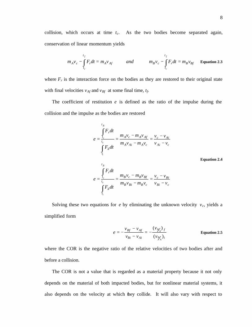
collision, which occurs at time tc. As the two bodies become separated again,
conservation of linear momentum yields
AfA
t
trcA vmdtFvm
f
c
=− ∫ and BfB
t
trcB vmdtFvm
f
c
=− ∫ Equation 2.3
where Fr is the interaction force on the bodies as they are restored to their original state
with final velocities vAf and vBf at some final time, tf.
The coefficient of restitution e is defined as the ratio of the impulse during the
collision and the impulse as the bodies are restored
cAi
Aic
cAAiA
AfAcAt
td
t
tr
vvvv
vmvm
vmvm
dtF
dtF
ec
i
fc
c
−−
=−
−==
∫
∫
cBi
Bic
cBBiB
BfBcBt
td
t
tr
vvvv
vmvm
vmvm
dtF
dtF
ec
i
fc
c
−−
=−
−==
∫
∫
Equation 2.4
Solving these two equations for e by eliminating the unknown velocity vc, yields a
simplified form
i
f
AiBi
AfBf
AB
AB
v
v
vv
vve
)(
)(−=
−
−−= Equation 2.5
where the COR is the negative ratio of the relative velocities of two bodies after and
before a collision.
The COR is not a value that is regarded as a material property because it not only
depends on the material of both impacted bodies, but for nonlinear material systems, it
also depends on the velocity at which they collide. It will also vary with respect to
9
different sizes, shapes and the temperature of the impacting bodies. For values of e=1,
the collision is considered to be a perfectly elastic impact, that is, there is no energy loss
due to the deformation of the bodies at impact. For values of e=0, the collision is
considered to be a perfectly plastic impact. The relative velocity of the two bodies after
impact is zero and the two particles move together at the same speed.
2.1.2 Mass Moment of Inertia and Parallel Axis Theorem
The mass moment of inertia is a measure of a body to resist a rotational acceleration
about an axis and is the best measure of how easily a bat can be swung. It is simply
denoted as MOI, noting that it refers to the mass moment of inertia and not to be
confused with an area moment of inertia. Studies described later have shown that batted-
ball velocity increases with increasing bat swing speed. Therefore, the MOI, because it is
an indicator of swing speed, can provide one measure of bat performance.
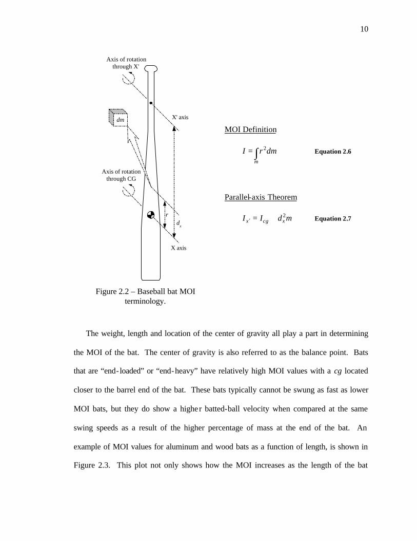
The definition of the MOI5 is simply a differential mass, dm, multiplied by the square
of the distance to an axis of rotation, r2, summed over the entire mass m, as defined by
Equation 2.6. The resulting units are MASS·DISTANCE2 (usually oz·in2 for baseball
bats). The MOI is traditionally calculated about an axis running through the center of
gravity, as illustrated in Figure 2.2, but using the parallel-axis theorem, the MOI can be
calculated about any arbitrary axis location, for example, the x´ axis, as defined in
Equation 2.7.
10
dm
r
Axis of rotationthrough CG
X' axis
X axis
Axis of rotationthrough X'
dx
Figure 2.2 – Baseball bat MOI
terminology.
MOI Definition
∫=m
dmrI 2 Equation 2.6
Parallel-axis Theorem
mdII xcgx2+=′ Equation 2.7
The weight, length and location of the center of gravity all play a part in determining
the MOI of the bat. The center of gravity is also referred to as the balance point. Bats
that are “end- loaded” or “end-heavy” have relatively high MOI values with a cg located
closer to the barrel end of the bat. These bats typically cannot be swung as fast as lower
MOI bats, but they do show a higher batted-ball velocity when compared at the same
swing speeds as a result of the higher percentage of mass at the end of the bat. An
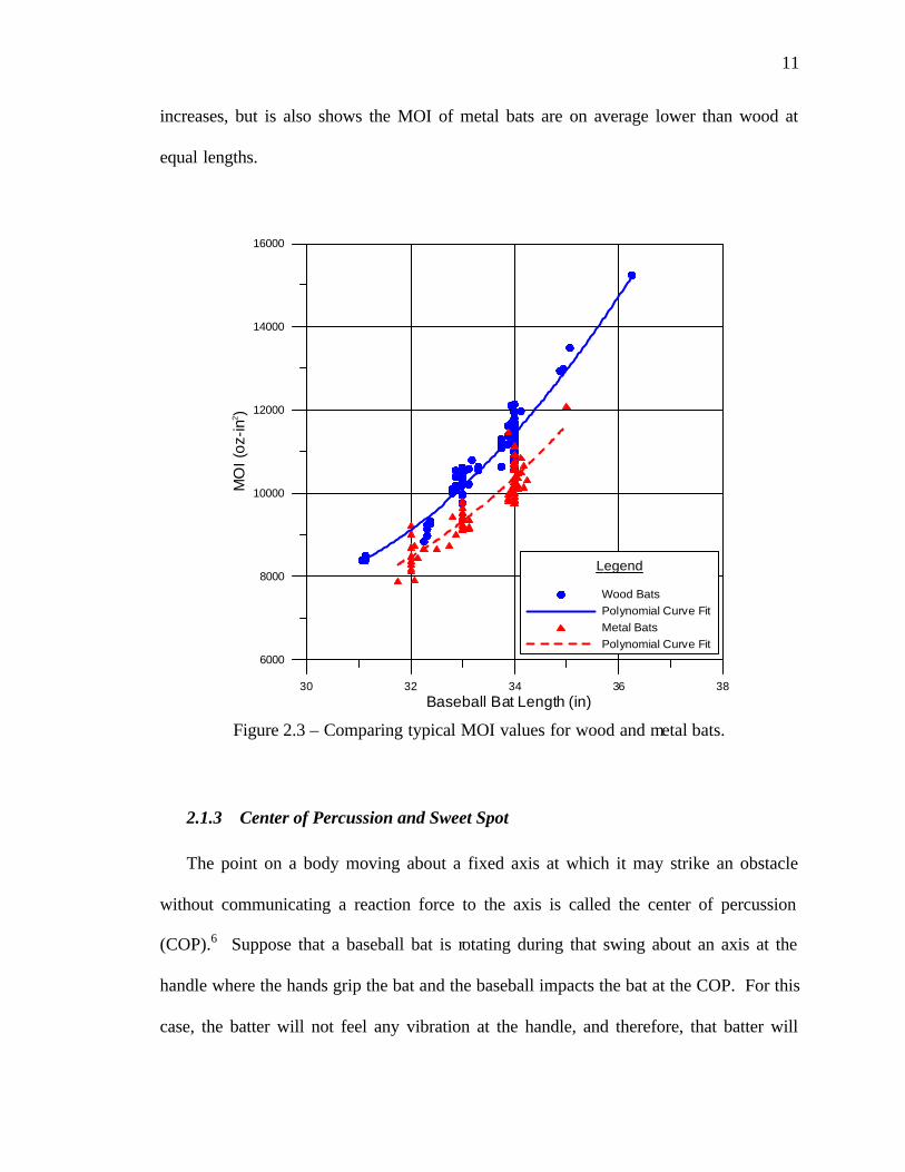
example of MOI values for aluminum and wood bats as a function of length, is shown in
Figure 2.3. This plot not only shows how the MOI increases as the length of the bat
11
increases, but is also shows the MOI of metal bats are on average lower than wood at
equal lengths.
30 32 34 36 38Baseball Bat Length (in)
6000
8000
10000
12000
14000
16000M
OI (
oz-in
2 )
Legend
Wood BatsPolynomial Curve FitMetal BatsPolynomial Curve Fit
Figure 2.3 – Comparing typical MOI values for wood and metal bats.
2.1.3 Center of Percussion and Sweet Spot
The point on a body moving about a fixed axis at which it may strike an obstacle
without communicating a reaction force to the axis is called the center of percussion
(COP).6 Suppose that a baseball bat is rotating during that swing about an axis at the
handle where the hands grip the bat and the baseball impacts the bat at the COP. For this
case, the batter will not feel any vibration at the handle, and therefore, that batter will
12
describe the collision as “hitting it on the sweet spot” of the bat. But the “sweet spot” can
also be defined as the location on the bat that will yield the maximum batted-ball
velocity, and does not necessarily coincide with the COP. There are vibration nodes
belonging to the 1st and 2nd bending modes of the bat that are also located in this general
area of the barrel (± 1 in) and it is suspected that they too have an affect on the batted-ball
velocity. Further experimentation should be done to quantify this effect.
2.2 Wood vs. Metal
The physical differences between wood and metal baseball bats are quite obvious. A
wood bat is solid, usually weighs 2 units less than its length and is not very durable. A
metal bat on the other hand, is hollow, weighs either 3 or more units less than its length
and is more durable than wood. A significant difference between wood and metal bats is
the energy-transfer mechanism between the bat and the baseball during the collision. The
difference between the energy-transfer mechanisms is a fundamental result of the wood
bat being solid and the metal bat being hollow.
2.2.1 The Bat-Ball Collision and Energy Transfer
In looking at the difference in performance between wood and metal bats, the generic
bat-ball collision must first be understood. This understanding includes the complex
motion of the bat to the ball and the energy transfer between the bat and the ball during
and after the collision. In his book The Physics of Baseball7, Adair reviews the
different aspects of a bat-ball collision. The complex motion of the bat towards the ball
is a combination of rotation and translation of both the batter and the bat. The swing is
mostly translation in the beginning stages and then mostly rotation just before hitting the
13
ball. However, the basic mechanics and motion of a swing will be the same whether the
batter is using a wood bat or a metal bat.
The total energy of a bat-ball collision is the sum of the kinetic energy generated by
the batter during the swing and the kinetic energy of the baseball pitched towards home
plate. When the ball collides with the bat, some energy is stored in the ball as it deforms
on the barrel to almost half of its original diameter. Some energy is stored in the bat as it
bends or deforms due to the impact with the ball, as shown in Figure 2.4. Some energy is
lost when frictional forces of the collision are dissipated through heat. However, the
amount of energy stored in the bat and how it is transferred back to the baseball is the
major difference between wood and metal baseball bats.
Figure 2.4 – An example of the bending deformation
of a baseball bat after it strikes the ball.
As previously noted, a metal bat is hollow. When the ball impacts the bat as shown
in Figure 2.5, the barrel elastically deforms and becomes oval in shape, storing energy
14
from the collision. When the material springs back to its original shape, the stored
energy in the bat is returned to the ball, propelling off of the bat at a faster rate than if
using a wood bat. Within this global hoop-deformation mode in hollow metal bats is a
phenomenon known as the trampoline effect. This trampoline effect is a local
deformation in the bat at the point of impact that also stores energy during contact with
the ball and then returns it to the ball as the bat returns to its original shape. The
trampoline effect also causes the baseball to deform less, which is significant because the
baseball is not a good energy storage device. When impacted with the solid wood bats,
the baseball deforms more, thus dissipating some of the collision energy.
TRAMPOLINEEFFECT
BEFORE IMPACT DURING IMPACT
HOOPMODE
Figure 2.5 – Bat-ball collision showing local trampoline
effect and global hoop deformation mode of metal bats.
By using newer metal alloys that have higher yield-strength, the trampoline effect can
increase the exit velocity of a baseball. Where the diameter profile along the length of a
solid wood bat is more of an artistic design, a metal bat is often engineered to give the
15
maximum performance possible, i.e. the fastest batted-ball velocity. The location of the
center of gravity, the moment of inertia, the sweet spot, the material selection, the
diameter profile, barrel reinforcements and the damping characteristics of a metal bat are
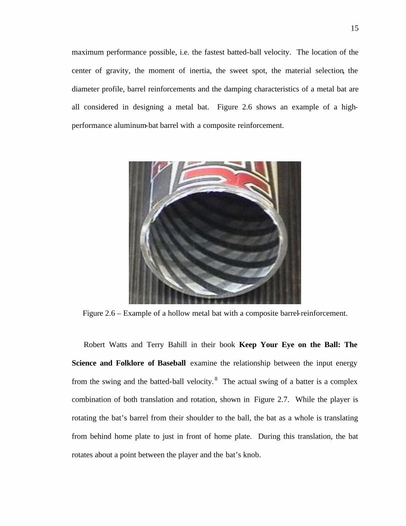
all considered in designing a metal bat. Figure 2.6 shows an example of a high-
performance aluminum-bat barrel with a composite reinforcement.
Figure 2.6 – Example of a hollow metal bat with a composite barrel-reinforcement.
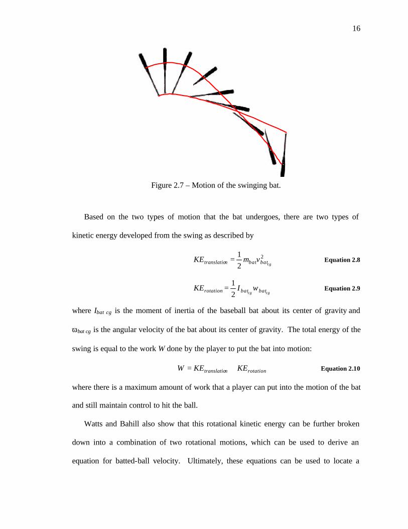
Robert Watts and Terry Bahill in their book Keep Your Eye on the Ball: The
Science and Folklore of Baseball examine the relationship between the input energy
from the swing and the batted-ball velocity. 8 The actual swing of a batter is a complex
combination of both translation and rotation, shown in Figure 2.7. While the player is
rotating the bat’s barrel from their shoulder to the ball, the bat as a whole is translating
from behind home plate to just in front of home plate. During this translation, the bat
rotates about a point between the player and the bat’s knob.
16
Figure 2.7 – Motion of the swinging bat.
Based on the two types of motion that the bat undergoes, there are two types of
kinetic energy developed from the swing as described by
2
21
cgbatbatntranslatio vmKE = Equation 2.8
cgcg batbatrotation IKE ω21
= Equation 2.9
where Ibat cg is the moment of inertia of the baseball bat about its center of gravity and
ωbat cg is the angular velocity of the bat about its center of gravity. The total energy of the
swing is equal to the work W done by the player to put the bat into motion:
rotationntranslatio KEKEW += Equation 2.10
where there is a maximum amount of work that a player can put into the motion of the bat
and still maintain control to hit the ball.
Watts and Bahill also show that this rotational kinetic energy can be further broken
down into a combination of two rotational motions, which can be used to derive an
equation for batted-ball velocity. Ultimately, these equations can be used to locate a
17
point on the bat that provides maximum energy transfer, in other words, highest batted-
ball velocity.
BodyRotation Axis
WristRotation Axis
CG
R H B
ωbody
ωwrist
Figure 2.8 – Variables denoted in swing equations.
Suppose that a batter’s swing can be drawn as shown in Figure 2.8 where two angular
accelerations are applied to the bat: ωbody due to the rotation of the body and ωwrist due to
the rotation of the batter’s wrists during the swing. The linear velocity of the bat at the cg
(v2b) and at the point of impact (vB) before a collision with the ball is
wristbodyB
wristsbodyb
BHBHRv
HHRv
ωω
ωω
)()(
)(2
++++=
++= Equation 2.11
Combining these two equations yields
bwristbodyB vBv 2)( ++= ωω Equation 2.12
Making the substitution of wristbody ωωω +=2 simplifies the equation further.
18
During the bat-ball collision, suppose that the force exerted on the bat from the
impact with the ball is –F1, resulting in a torque on the bat about its cg is equal to –BF1.
Equating this torque over time t to the change in angular momentum yields for the bat
)( 2201 baItBF ωω −=− Equation 2.13
Similarly for the ball
)( 1111 ba vvBmtBF −= Equation 2.14
Assume that the rotational kinetic energy of the ball is negligible when compared to
the translational kinetic energy. Conserving angular momentum between the bat and the
ball during the collision produces
0)()( 111220 =−+− baba vvBmI ωω Equation 2.15
Recall that Equation 2.1 and Equation 2.5 also apply to the energy stored during a
bat-ball collision. It should be noted that Equation 2.5 is modified here to represent the
fact that the impact is not at the cg location of the bat, such that the COR is defined as
bbb
aaa
BvvBvv
e221
221
ωω
−−−−
−= Equation 2.16
Equations 2.1, 2.15 and 2.16 can now be solved simultaneously to find the batted-ball
velocity v1a.
0
21
2
1
220
21
2
11
1
1
))(1(
IBm
mm
BveIBm
mm
ev
vbbb
a
++
+++
−−−
=
ω
Equation 2.17
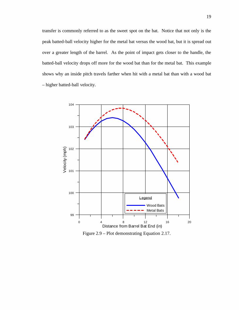
By substituting into Equation 2.17 representative values for wood and metal bats, a
plot of the batted-ball velocity as a function of the location of the impact point on the bat
from the barrel end can be created. The peaks of Figure 2.9 show where along the length
of the bat the maximum energy transfer occurs. This location of maximum energy
19
transfer is commonly referred to as the sweet spot on the bat. Notice that not only is the
peak batted-ball velocity higher for the metal bat versus the wood bat, but it is spread out
over a greater length of the barrel. As the point of impact gets closer to the handle, the
batted-ball velocity drops off more for the wood bat than for the metal bat. This example
shows why an inside pitch travels farther when hit with a metal bat than with a wood bat
– higher batted-ball velocity.
0 4 8 12 16 20Distance from Barrel Bat End (in)
99
100
101
102
103
104
Vel
ocity
(mph
)
Legend
Wood BatsMetal Bats
Figure 2.9 – Plot demonstrating Equation 2.17.
20
2.3 Performance Statistics of Wood vs Metal
There is much anecdotal evidence of how a metal bat outperforms the traditional
wood bat. Two studies are selected here to demonstrate some empirical evidence.
2.3.1 Thurston’s Cape Cod League Study
In Thurston’s study, he examined several offensive statistics: batting average,
slugging percentage, home runs per at bat, base on balls per at bat, strikeouts per at bat,
runs scored per at bat and runs batted in (RBI) based on percent runs driven in per at bat.
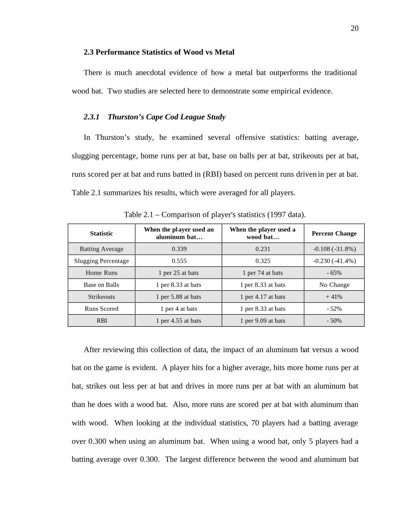
Table 2.1 summarizes his results, which were averaged for all players.
Table 2.1 – Comparison of player's statistics (1997 data).
Statistic When the pl ayer used an
aluminum bat… When the player used a
wood bat… Percent Change
Batting Average 0.339 0.231 -0.108 (-31.8%)
Slugging Percentage 0.555 0.325 -0.230 (-41.4%)
Home Runs 1 per 25 at bats 1 per 74 at bats - 65%
Base on Balls 1 per 8.33 at bats 1 per 8.33 at bats No Change
Strikeouts 1 per 5.88 at bats 1 per 4.17 at bats + 41%
Runs Scored 1 per 4 at bats 1 per 8.33 at bats - 52%
RBI 1 per 4.55 at bats 1 per 9.09 at bats - 50%
After reviewing this collection of data, the impact of an aluminum bat versus a wood
bat on the game is evident. A player hits for a higher average, hits more home runs per at
bat, strikes out less per at bat and drives in more runs per at bat with an aluminum bat
than he does with a wood bat. Also, more runs are scored per at bat with aluminum than
with wood. When looking at the individual statistics, 70 players had a batting average
over 0.300 when using an aluminum bat. When using a wood bat, only 5 players had a
batting average over 0.300. The largest difference between the wood and aluminum bat
21
can be seen in the 65% decrease in home runs per at bat. Fifty-eight players had at least
one home run every 40 at bats when they used an aluminum bat, while only 16 players
had the same success when they used a wood bat. The increase of strikeouts per at bat
from 0.17 with aluminum bats to 0.24 with wood bats could be a measure of swing speed,
in that a player can swing an aluminum bat faster than he can swing a wood bat. Also,
the lower MOI of an aluminum bat gives the batter better control to move the bat up and
down in the strike zone as he swings. The slower swing speed with a wood bat may not
allow a hitter to catch up to a fastball and make contact. In addition, to make up for the
slower swing speed with wood, the batter has to commit his swing earlier than he would
with an aluminum bat. If a batter can wait until the last possible moment before starting
his swing, he has the better chance of making contact with the ball. The earlier a batter
commits to swinging at a pitched ball, the less chance he has at making contact because
he basically is guessing at where the ball will be. The runs scored and runs batted in per
at bat were cut in half when the players used wood bats. The ball is put in play more with
a metal bat than with a wood bat, resulting in a greater chance of scoring a run.
2.3.2 Sports Engineering Field Performance Study
With assistance from UMass Lowell's Baseball Research Center (UMLBRC), Larry
Fallon of Sports Engineering conducted several field performance studies that compared
the distance a ball travels when hit with professional quality wood bats versus aluminum
bats. The two C405 aluminum bats used in the study were from two different
manufacturers and were both -5 bats. In these studies, approximately 40 Rookie and
Single-A class players from two Major League Baseball organizations used wood and
aluminum bats while taking their regular batting practice drills. The baseball field was
22
measured and flags were positioned radially from home plate eve ry 10 ft starting at 250 ft
and ending outside the outfield fence at 450 ft. The distance a ball traveled in the air to
where it first landed was recorded to an accuracy of 5 ft.
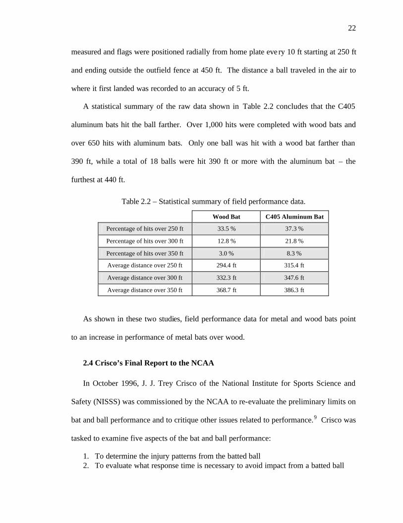
A statistical summary of the raw data shown in Table 2.2 concludes that the C405
aluminum bats hit the ball farther. Over 1,000 hits were completed with wood bats and
over 650 hits with aluminum bats. Only one ball was hit with a wood bat farther than
390 ft, while a total of 18 balls were hit 390 ft or more with the aluminum bat – the
furthest at 440 ft.
Table 2.2 – Statistical summary of field performance data.
Wood Bat C405 Aluminum Bat
Percentage of hits over 250 ft 33.5 % 37.3 %
Percentage of hits over 300 ft 12.8 % 21.8 %
Percentage of hits over 350 ft 3.0 % 8.3 %
Average distance over 250 ft 294.4 ft 315.4 ft
Average distance over 300 ft 332.3 ft 347.6 ft
Average distance over 350 ft 368.7 ft 386.3 ft
As shown in these two studies, field performance data for metal and wood bats point
to an increase in performance of metal bats over wood.
2.4 Crisco’s Final Report to the NCAA
In October 1996, J. J. Trey Crisco of the National Institute for Sports Science and
Safety (NISSS) was commissioned by the NCAA to re-evaluate the preliminary limits on
bat and ball performance and to critique other issues related to performance.9 Crisco was
tasked to examine five aspects of the bat and ball performance:
1. To determine the injury patterns from the batted ball 2. To evaluate what response time is necessary to avoid impact from a batted ball
23
3. To evaluate existing test methods for predicting ball performance 4. To evaluate existing test methods for predicting bat performance 5. To determine the effects of bat mass and inertia on swing velocity
Crisco’s year- long study encompassed much of the recent work done on investigating
the performance of baseball bats by collecting many “papers in progress” and enlisting
other facilities to conduct supporting research. Because of the extent of his study, its
conclusions are used here as a guide.
2.4.1 Relationship between Reaction Time and Injuries due to the Batted Ball
Based on data from the NCAA Injury Surveillance System, Crisco concluded that
baseball had one of the lowest overall injury rates in any collegiate sport. The acceptable
risk of receiving an injury due to a batted ball had yet to be determined and the exact
level of acceptability should be established using values determined from scientific
studies. Also, the existing standards of bat and ball performance as it relates to injuries
were based on practical experience with little scientific basis.
With respect to quantifying the relationship between reaction time and injuries due to
batted balls, Cassidy and Burton10 examined research literature on the reaction time of
baseball players and the amount of time it takes for a player to move an arm to a
defensive position. They concluded that the average college or professional player is able
to begin their response to the ball 125 ms after the ball is impacted and that it takes
approximately 200 ms to complete the arm movement for a defensive position. Based on
these two findings, a player is calculated to have approximately 325 ms to react to a
batted ball and move his arm to catch or block the ball. This value has become quite
controversial.
24
A pitcher is typically 55 ft from home plate when he finishes delivering the ball to the
catcher. Suppose that a ball is then hit directly back at the pitcher. Based on the 325 ms
reaction time, if a batter hits a line drive up the middle, then the pitcher would not have
enough time to react to the ball if it was traveling at 115 mph or faster. This calculation
neglects any drag on the ball due to air resistance, so the actual velocity could be slightly
less than 115 mph. Regardless, this ball exit velocity was much higher than any wood
bat, yet pitchers are still hit by line drives off wood bats. Scientists at the NCAA’s July
1998 bat summit agreed that approximately 400 ms, not 325 ms was necessary for a
pitcher to defend himself against a line drive.11 That would reduce the “safe” ball exit
velocity to 93.75 mph. Crisco noted that although injuries from balls hit with wood bats
have also occurred, the severity of the injury seems to increase with increasing ball
velocity. In other words, a pitcher hit with a ball coming off an aluminum bat would
suffer a more serious injury than if the bat were made of wood because the ball would be
traveling at a higher velocity with more kinetic energy to release in the collision.
2.4.2 Predicting Ball Performance
Because the performance of a baseball bat is usually quantified by the exit speed of
the batted ball, the performance of the baseball should also be quantified. Suppose two
different lots of baseballs from a single manufacturer were used for testing. One lot has a
high COR value (“juiced” or lively balls) and the other has a much lower COR value
(“dead” balls). If the “juiced” balls were used to test a wood bat, and the “dead” balls
were used to test a metal bat, the relative performance of the wood and metal bats could
be equal. On the other hand, if the “juiced” balls were used to test the metal bat instead,
then the relative performance of the metal bat could be artificially inflated. This simple
25
example shows that you cannot address the performance of a baseball bat without also
considering the performance of the baseball.
2.4.2.1 COR Testing
As of 1999, the specification regarding collegiate- level ball performance is that the
baseball must have a COR between 0.525 and 0.555. Currently, the specification is that
the COR must be less than or equal to 0.555 for a ball impacting a stationary wall at an
initial velocity of 85 ft/sec (58 mph). The physical specifications on baseballs used in
NCAA games are: a ball shall weigh no less than 5 oz and no more than 5.25 oz; the
circumference of the baseball shall be no less than 9 in and no more than 9.5 in. The
final stipulation is that the ball shall be formed by yarn wrapped around a small core of
rubber, cork or a combination of the two, and it shall be covered by two pieces of white
horsehide or cowhide tightly stitched together.
The current test method for measuring the COR is ASTM 1887, Standard Test
Method for Measuring the Coefficient of Restitution (COR) of Baseballs and Softballs.12
It uses a ball-throwing device, for example a pitching machine, to propel a ball towards a
fixed, flat wall. The velocity of the ball just before impact is 58 mph and the strike plate
is made from either 2- inch thick steel or 4- inch thick northern white ash. The velocity of
the ball before and after impact is measured using a set of electronic speed gates set 12
inches apart, and the COR is then calculated as the incoming speed divided by the
rebound speed.
Crisco noted that the major limitation of the ASTM COR test is the unrealistic
inbound velocity of 58 mph. Realistic pitch velocities for a college game range from 75
to 85 mph and bat swing speeds are in the 70 mph range (i.e., the linear velocity of the
26
bat at the point of impact is 70 mph). The total collision speed would be the sum of the
two, equal to 150 mph, well above the experimental speed of 58 mph. There is some
debate as to whether this COR test can accurately predict ball performance because the
test uses a flat surface, not a cylindrical surface simulating a baseball bat barrel. Given
that there are many factors which influence the COR of a baseball, Crisco concluded that
the current specification is insufficient for predicting ball performance at realistic
velocities.
2.4.2.2 Ball Compression Testing
A baseball is a complex object consisting of nonlinear materials such as leather, yarn,
rubber and cork. A cross-section of a baseball is shown in Figure 2.10. Because the ball
is nonlinear, it is difficult to quantify baseball field performance other than using a COR
test at elevated game speeds. One attempt to supplement the COR testing is to quantify
the nonlinear stiffness of baseballs using a compression test, an example of which is
shown in Figure 2.11.
27
Figure 2.10 – Cross-section of a baseball.
Figure 2.11 – An example of the ASTM ball compression test and resulting data.
ASTM 1888, Standard Test Method for Compression-Displacement of Baseballs and
Softballs13 uses a static compression test to measure the load reached when the ball is
compressed 0.25 in between two flat plates. It is a relatively easy test to perform, and it
gives a quantitative measure of ball hardness. Unfortunately, it is difficult to extrapolate
the ball compression from a static event (0.25 inches of displacement over 12 to 15
28
seconds) and apply it to a highly dynamic event of a bat-ball collision where the ball is
compressed and returns to its original shape in less than 100 milliseconds. Test results
from two different ball manufacturers are shown in Table 2.3. The difference between
the maximum loads reached between the two sets of 6 baseballs was 68.1 lb. This
variation has been observed in experimental batted-ball velocity measurements, where
one ball has a higher average exit velocity than another ball when hit with the same bat.
However, the potential correlation between a static ball compression test and the dynamic
batted-ball velocity is not fully documented and is not covered in this thesis.
Table 2.3 – Ball compression test results.
Ball Manufacturer & Model Rawlings R1NCAA Wilson A1001SST
Average Weight (oz) 5.108 5.101
Average Load (lb) 353.4 421.5
2.4.3 Predicting Bat Performance
There are two testing methodologies considered for predicting baseball bat
performance. The first is ASTM 1991, Standard Test Method for Measuring Baseball
Bat Performance Factor14 as developed by New York University physicist Dr. Richard
Brandt, Ph.D. It uses a value called the Bat Performance Factor, or BPF, which is a ratio
of the COR of a bat-ball collision and the COR of the same ball impacting a flat, rigid
wall. The second methodology uses the Baum Hitting Machine (BHM), developed by
Baum Research and Development. This machine uses large servomotors to swing a bat
and a ball toward each other at specified velocities and then measures the exit velocity of
the batted-ball after impact.
29
2.4.3.1 Brandt Test and the BPF
The Brandt test uses an air cannon to impact a cantilevered bat on a freely rotating
turntable with a baseball, as shown in Figure 2.12. By measuring the inbound velocity of
the baseball before impact and then measuring the rebound velocity of the bat after
impact, the bat-ball COR is calculated using Equation 2.18:
11 2 −
+=− drT
DRtwR
ICOR ballbat Equation 2.18
where:
D = distance between bat-speed sensors (in) d = distance between ball-speed sensors (in) I = moment of inertia (oz-in2) R = location of the center of percussion (in) r = radius of bat speed sensors (in) T = time for bat to travel through bat speed sensors (s) t = time for ball to travel through ball speed sensors (s) w = weight of ball used in test (oz)
Air
Can
non
Speed gatesto measureinbound ballvelocity
Speed gatesto measurereboundingbat velocity
Figure 2.12 – Schematic of Brandt test setup.
30
The BPF is then calculated as the CORbat-ball divided by the ball COR as found using
ASTM 1887. The batted-ball speed can then be related to BPF by:
( ) ( )( )k
keveVV ball batted +
−++=
11
Equation 2.19
( )( )
−−
+
= 2
2
1 WaaRw
Ww
k Equation 2.20
where:
V = bat speed (mph, measured at point of impact at COP of bat) v = pitch speed (mph) w = ball weight (oz) W = bat weight (oz) I = moment of inertia (oz-in2) e = bat-ball COR (equal to BPF·CORball) a = distance from pivot to bat center of mass or balance point (in) R = location of COP (in) k = bat-ball inertia ratio (grouping term)
Crisco notes that although the Brand t method has gained wide acceptance, it does not
test bat performance at realistic game velocities. Measurements are made at 60 mph and
mathematically extrapolated to the desired elevated velocity. Typical values range from
1.0 for wood bats to 1.14 for metal bats. On the other hand, the BHM can test at any
combination of velocities, up to a combined 200 mph, and directly measure the COR at
these velocities.
2.4.3.2 Baum Hitting Machine
Larry Fallon of Sports Engineering, Dr. James Sherwood of the University of
Massachusetts, Lowell and consultant Dr. Robert Collier, were commissioned by MLB to
perform a complete and thoroughly independent evaluation of the BHM.15 This UMass
Lowell group also proposed a standard protocol using the BHM to evaluate the
31
performance of baseball bats. They concluded that the BHM is a state-of-the-art machine
capable of accurately measuring ball exit velocity. The BHM, shown in Figure 2.13 has
the capability of swinging a bat at speeds up to 100 mph at the contact point and pitching
a ball at up to 100 mph.
(a) (b)
(c) (d)
Figure 2.13 – Assorted views of the BHM.
The operator controls the BHM’s movements by setting the coordinates of the bat-
ball impact and individual speeds of the bat and ball and records the impact data from the
control area, as shown in Figure 2.13(a). The bat-ball impact setup is observed as shown
in Figure 2.13(b). A baseball bat is mounted in the bat holding fixture that sits atop one
of the motors, while the ball is held in place in the ball “tuning fork” fixture attached to
the other motor shown in Figure 2.13(c). Sets of light cells and speed gates measure the
32
exit velocity of the ball as it moves away from the impact. The ball is eventually stopped
by the collection net shown in Figure 2.13(d).
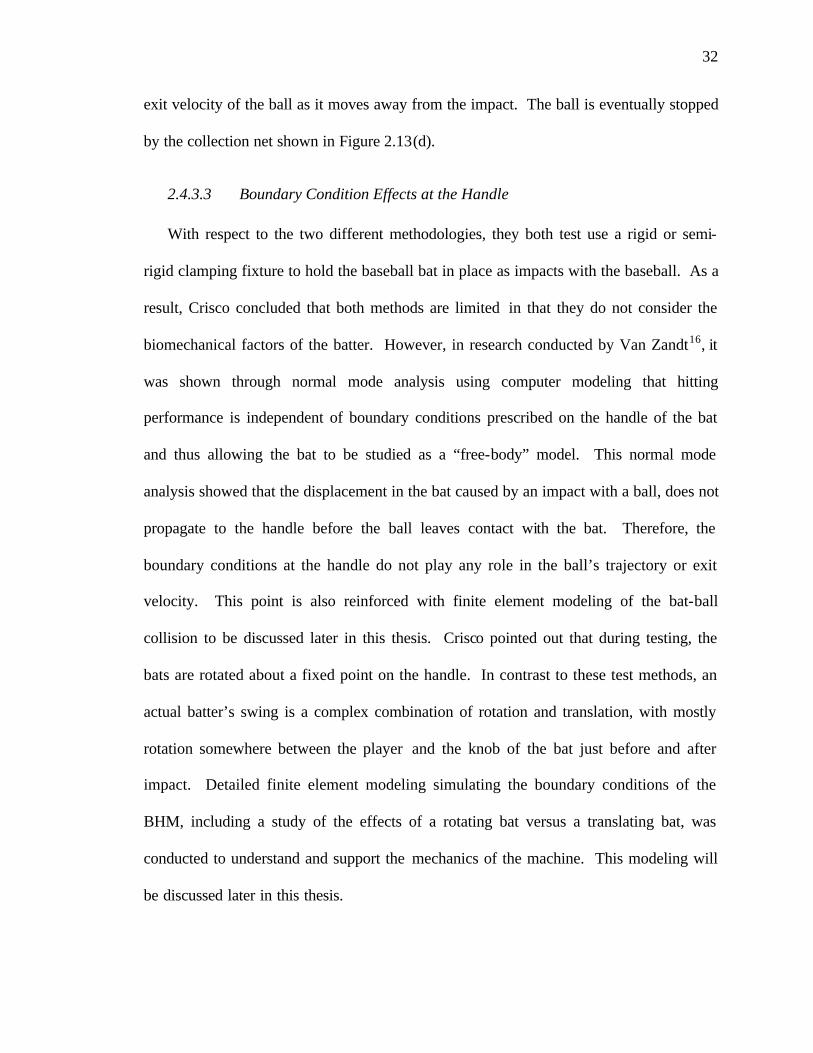
2.4.3.3 Boundary Condition Effects at the Handle
With respect to the two different methodologies, they both test use a rigid or semi-
rigid clamping fixture to hold the baseball bat in place as impacts with the baseball. As a
result, Crisco concluded that both methods are limited in that they do not consider the
biomechanical factors of the batter. However, in research conducted by Van Zandt16, it
was shown through normal mode analysis using computer modeling that hitting
performance is independent of boundary conditions prescribed on the handle of the bat
and thus allowing the bat to be studied as a “free-body” model. This normal mode
analysis showed that the displacement in the bat caused by an impact with a ball, does not
propagate to the handle before the ball leaves contact with the bat. Therefore, the
boundary conditions at the handle do not play any role in the ball’s trajectory or exit
velocity. This point is also reinforced with finite element modeling of the bat-ball
collision to be discussed later in this thesis. Crisco pointed out that during testing, the
bats are rotated about a fixed point on the handle. In contrast to these test methods, an
actual batter’s swing is a complex combination of rotation and translation, with mostly
rotation somewhere between the player and the knob of the bat just before and after
impact. Detailed finite element modeling simulating the boundary conditions of the
BHM, including a study of the effects of a rotating bat versus a translating bat, was
conducted to understand and support the mechanics of the machine. This modeling will
be discussed later in this thesis.
33
2.4.4 Effects of Bat Mass and Inertia
The length-to-weight unit difference is a bat property that is restricted by NCAA
rules. It should be noted that the length-to-weight unit difference could be no more than
5 (measured with the grip) at the time of Crisco's report in November 1997; it was
changed to no more than 3 (measured without the grip) effective January 1999. Two
studies reviewed here show that the moment of inertia (MOI) has a more dominant effect
on swing velocity than weight. These studies calculated the MOI about a point on the
batter's body located 20 in from the knob end of the bat. They showed that swing speed
increased as bat MOI decreased and that over the small range of swing velocities they
examined, the relationship between swing speed and MOI was assumed to be linear.
2.4.4.1 Effect of Bat Mass and Inertia on Swing Speed
Fleisig, et al.17 at the American Sports Medicine Institute (ASMI) investigated the
effect of bat mass and inertia on swing velocity by using a high-speed motion-analysis
system to measure the swing speed of a baseball bat. They examined the swing speeds of
17 collegiate players using regular aluminum bats and aluminum bats modified by
placing a large or small weight at the barrel or the handle. The players then used the bats
in a controlled environment, batting balls pitched from a baseball pitching machine. The
pitch speed was approximately 58 mph and the machine was located 42 ft from home
plate. A statistical analysis of the measured linear velocity of the sweet spot and angular
velocity of the bat was then performed.
The ASMI group found that bat swing speeds increased as the bat MOI decreased.
This finding was based on the linear velocity data because an ANOVA analysis revealed
significant differences among the linear velocities but not for the angular velocities.
34
Based on the regression, the bat speed (linear velocity of the sweet spot in mph) can be
predicted by:
IV ⋅−= 7.486.69 Equation 2.21
where I is the MOI about the bat handle in units of lbf⋅ft⋅s2.
2.4.4.2 A Method to Measure Swing Speed
Koenig, et al. 18 at Mississippi State University (MSU) used 20 college-level players
and measured their swing speeds using sensors mounted in the ground at home plate.
The baseball bats used in this study were a mix of regular high-performance aluminum
bats and modified bats with a weight located on the inside of the bat barrel or handle.
The lengths of all the bats were 34 in, thus the unit difference between the weight and
length of each bat was achieved by altering the weight of the bat. Baseballs were pitched
from a baseball pitching-machine at 64 mph located 48 ft from home plate. Baseballs
were also hit off a tee. Bat-speed data was collected and fitted to least-square linear
curves based on relationships between MOI versus bat speed and the length-to-weight
unit difference versus bat speed.
Comparing the bat speeds for pitched versus tee-ball swings, the data for the pitched
ball show that there was a slight decrease in bat speed as the MOI increases, while there
was no change in bat speed for balls hit off the tee. The MSU group relates these linear
curve fits to the MOI using the physical parameters involved in swinging the bat. To
idealize the actual swinging of a baseball bat, they assume that the bat's motion is starting
from rest and is in pure rotation about a fixed axis. They conclude that the changes in bat
speed (in mph) as a linear function of the changes in MOI from bat to bat can be
expressed by:
35
∆−⋅⋅=∆
ref
bat
ref II
IT
rV2
12θ
Equation 2.22
where θ2r ⋅ relates the angular and radial position of the sensors; refITθ2
is a measure
of the angular velocity that a batter can give to a reference bat with an MOI of Iref by
applying a torque T; and
∆−
ref
bat
II
21 is the amount of change in the angular velocity due
to changes in MOI. In layman's terms, the MSU group notes that a 10% increase in the
MOI will result in a 4-mph decrease in bat speed over the outside of home plate for
swings at pitched balls. It is noted that all bat-speed measurements are made from the
outside edge of home plate, not at any specific point on the baseball bat. Additional
sensors could be located at different positions at home plate in order to measure different
points on the bats.
2.4.4.3 The Ideal Bat Weight
Watts and Bahill19 discuss what the ideal bat weight should be in order to get the
maximum batted-ball velocity. The conservation of momentum and COR equations for