NBER WO~G PAPER SERIES A MODEL OF FOREIGN EXCHANGE RATE ~DETERM~ATION Charles Engel Working Paper 5766 NATIONAL BUREAU OF ECONOMIC RESEARCH 1050 Massachusetts Avenue Cambridge, MA 02138 September 1996 I appreciate helpfal comments from a number of colleagues in the field. Some of the work on this paper was completed while I was a visiting scholar at the Federal Reserve Bank of Kansas City. The views expressed in this paper are my own and are not necessarily shared by the Federal Reserve Bank of Kansas City or the National Bureau of Economic Research. I acknowledge assistance from the National Science Foundation, NSF grant #SBR-932078. This paper is part of NBER’s research program in International Finance and Macroeconomics, and NBER’s project on International Capital Flows. We are gratefil to the Center for International Political Economy for the support of this project. hy opinions expressed are those of the author and not those of the National Bureau of Economic Research. 01996 by Charles Engel. All rights reserved. Short sections of text, not to exceed two paragraphs, may be quoted without explicit permission provided that fall credit, including O notice, is given to the source,
Transcript
NBER WO~G PAPER SERIES
A MODEL OF FOREIGN EXCHANGERATE ~DETERM~ATION
Charles Engel
Working Paper 5766
NATIONAL BUREAU OF ECONOMIC RESEARCH1050 Massachusetts Avenue
Cambridge, MA 02138September 1996
I appreciate helpfal comments from a number of colleagues in the field. Some of the work on thispaper was completed while I was a visiting scholar at the Federal Reserve Bank of Kansas City. Theviews expressed in this paper are my own and are not necessarily shared by the Federal ReserveBank of Kansas City or the National Bureau of Economic Research. I acknowledge assistance fromthe National Science Foundation, NSF grant #SBR-932078. This paper is part of NBER’s researchprogram in International Finance and Macroeconomics, and NBER’s project on International CapitalFlows. We are gratefil to the Center for International Political Economy for the support of thisproject. hy opinions expressed are those of the author and not those of the National Bureau ofEconomic Research.
01996 by Charles Engel. All rights reserved. Short sections of text, not to exceed two paragraphs,may be quoted without explicit permission provided that fall credit, including O notice, is given tothe source,
NBER Working Paper 5766September 1996
A MODEL OF FOREIGN EXCHANGERATE ~DETERMINATION
ABSTRACT
Economic agents undertake actions to protect themselves from the short-run impact of
foreign exchange rate fluctuations: Nominal goods prices are set in consumers’ currencies, and firms
hedge foreign exchange risk. A model is presented here which shows that these features of the
economy can lead to indeterminacy in the nominal exchange rate in the short run. There can be
noise in the exchange rate, unrelated to any fundamentals, essentially because the short-run
fluctuations do not influence any rational agent’s behavior. Empirical implications of this sort of
noise are explored.
Charles EngelDepartment of EconomicsUniversity of WashingtonSeattle, WA 98195and [email protected]~ GTON.EDU
Since the collapse of the Bretton Woods system in the early 1970s, nominal exchange
rates among industrialized countries have been extremely volatile. The short-run
movements in exchange rates have b=n much more extreme than early proponents of floating
rams (such as Friedman (1953) and Johnson (1972)) envisaged.
Two notable puzzles that arise in relation to this volatility are:
(1) What accounts for the volatility? Some of the tharetical models of the 1970s were
specifically designed to explain how the nominal exchange rate could be much more
volatile than the underlying economic fundamentals (notably Dombusch (1976)). But these
models have fared very badly empirically. Meese and Rogoff (1983a, 1983b), and
subsequently many others, have documented the failure of these models in explaining
short-run movements of exchange rates. While the models are more successful at longer
horizons (Mark (1995), Chinn and Meese (1995)), the movement of exchange rates at short
horizons seems independent of the movement in what are hypothesized to be the underlying
economic fundamentals (Flood and Rose (1995)).
(2) Despite the huge variability in nominal exchange rates, international trade does not
appear to have b=n greatly adversely affwted (see, for example, Kroner and Lastrapes
(1993)), On the contrary, there has been a steady opening of markets and expansion in
the volume of trade.
The story of this paper is simple: In the short run, nominal exchange rate changes
have essentially no rd effwts. But, since a change in the exchange rate does not
affect any agent’s behavior, the level of the exchange rate is indeterminate. Purely
extrinsic noise causes the exchange rate to fluctuate around the equilibrium value
determined by the fundamentals.
There are two essential elements to the model presented here. First, recent work
has noted that nominal exchange rate fluctuations have little effect on the prices
1
consumers pay (Knetter (1989, 1993), Engel (1993), Engel and Rogers (1996)). There
appears to be forces of both pricing to market and nominal price stickiness at work in
international markets. Producers charge different prices for similar goods in different
markets. A German producer might charge one price for its product at home, and another
prim for sale in the U.S. The reasons for this type of price discrimination have b~n
explored extensively in r=nt literature (see, for example, Krugman (1987), Dombusch
(1987), Marston (1990)). Prices may not respond to exchange rate changes either for
reasons explored in the “pass-through” literature, or because there are menu-costs to
changing prices (such as in Mankiw (1985)).
While nominal price stickiness has bwn a feature of a long line of models of
exchange rates, generally the price stickiness in these models is of a different sort
than has ban observed in the data. Dombusch (1976), for example, assumes that
exporters set prices in their own currencies. If the dollar depreciates relative to the
mark, imports from Germany become more expensive for Americans in the Dombusch
formulation. But, the evidence suggests that, because firms price to market, they set
the price in the currency of the country that buys the good. German firms set the price
of their exports to the U.S. in dollar terms. A change in the exchange rate has no
effect on that price in the short run. 1
There is an effmt on the profits of a German firm, however, if the dollar
deprmiates and the German firm’s export price is fixed in dollars. The revenue per item
sold will decline in mark terms. The German firm’s profits are adversely tifected. But,
that leads to the second essential element of the model in this paper. Firms can hedge
against exchange rate fluctuations. A sufficiently insured firm can fully hedge against
losses from exchange rate fluctuations that are purely noise.
1 Some of the evidence in the pricing-to-market literature suggests that U. S firmsare different than other firms in their pricing behavior. But, Rangan and Lawrence(1993) argue that this is an incorrect inference based on faulty data.
2
Ind4, in the simple model presented here, all fluctuations in the exchange rate
are extrinsic. The exchange rate moves at the whim of foreign exchange traders. But
that noise affects nobody. Consumers are unaffectd because the prices they face are
fixed and unresponsive to exchange rate changes. The exchange rate risk that firms face
is fully diversifiable. The firms simply make contracts that s~ify that the winners
from exchange rate changes pay off the losers. Since the exchange rate fluctuations have
no other real effects, the firms desire these contracts -- their expected return is
unchanged by the contracts, but the risk from exchange rate fluctuations is eliminated.
The model in this paper is different than other raent models of exchange rate
indeterminacy (e. g., King, Wallace and Webcr (1992), Manuelli and P-k (1990)). Here,
the indeterminacy arises from two specific observable features of the international
economy -- pricing-to-market and hedging of exchange rate risk. The idea of this paper
does build naturally on the notion that pricing to market increases exchange rate
volatility in equilibrium (Krugman (1989), Betts and Devereux (1996)). In the model of
this paper, there is “excess” volatility, in the sense that purely extrinsic noise
affects the exchange rate.
Section 1 presents a simple static general equilibrium model of two countries with
a large number of firms selling products at home and abroad. The model is one with
flexible prices and a determinate exchange rate. Its purpose is to determine the
expected prices and exchange rates that firms and consumers face. In section 2, we
rquire that prices be set in advance of the determination of the exchange rate. Prices
will be set at the quilibrium level from section 1. Firms will also make contracts to
hedge the risk of the exchange rate ending up at some level other than the expected rate
from the model of section 1. The exchange rate will be seen to be indeterminate.
Section 3 discusses some of the empirical implications of this model. One is that
there will be little relation betwmn exchange rates and fundamentals in the short run,
3
but that they will be closely related in the long run, Other possible avenues for
empirical work for future versions of this paper are discussed. The section also
mnsiders implications of this model for other issues, such as the responsiveness of
trade to exchange rate changes, and the choice of nominal exchange rate regime.
There is one major determinant of exchange rates that the model ignores -- the role
of speculation in stabilizing the exchange rate. In the model, the exchange rate is
influenced by extrinsic noise in the short-run, which implies that there is an expected
profit opportunity for speculators who bet that the exchange rate will return to its
fundamental value. This speculation ought to help nail down the exchange rate. On the
other hand, hundreds of studies of forward foreign exchange rate market efficiency have
documented the empirical regularity that the forward rate is a biased predictor of future
spot rates, and have made essentially no progress in explaining this bias with models of
rational risk-averse economic agents (SW Hodrick (1987) and Engel (1996) for
comprehensive surveys. ) It is difficult to reject the conclusion that foreign exchange
market s~ulators do allow expected profit opportunities to go unexploited. But, this
paper does not attempt to tackle that difficult subjwt: it sidesteps it completely. It
s=ms likely, however, that the issues raised here concerning how economic agents protmt
themselves from the effats of foreign exchange rate fluctuations could play a role in
future research into understanding the efficiency or inefficiency of international
capiti markets.
1. The Equilibrium Model
The model is of two countries, call them the U.S. and Germany, that are identicd
in the sense that consumers have the same utility functions, producers have the same
4
production functions, and the economies are of the same size. This is a model with no
uncertainty.
Consumer$
Consumers in the U.S. maximize
1 l-R + &.(M’d/p)l-RU=nQ + &(l-L)l-R. o< @<l
where
In this function, ~ is consumption of good i. The range from O to 1/2 are
produced irl the U. S., and the goods indexed from 1/2 to 1 are produced in Germany. Md is
the nominal quantity of money demanded by Americans. L is supply of labor.
P is defined by
Some points about the utility function can be briefly noted. All goods enter
utility symmetrically. The restriction that #1lie between zero and unity is nmessary
for an equilibrium with monopolistic producers of each good. Rd balances appear in the
utility function as a simple way of capturing the transactions
R can be interpreted as the measure of relative risk aversion
The budget constraint faced by an American
f}i~di + Md =wL+M+ IT,
The price of good i is pi. All of these prices are
wage rate paid in competitive labor markets is w.
is
expressed
motive for holding money.
for consumers.2
in terms of dollars. The
All individuals receive a transfer of
money, M. Finally, all individuals are endowed with equal ownership in each of the
American firms. II is the amount of profits paid to the representative American.
2 See the discussion on risk aversion and risk neutrality with multiple goods inEngel (1992).
5
The first-order conditions for goods, money and labor demands imply:
qi = @i/P)-l’@Q,
Md = PQelm,
L = 1 - Q(P/w)lm.
Symmetridy, the optimization problem faced by Germans is to maximin
u“ = &Q ●l-R + &.(M*d/p”)l-R + &(l-L*)l-R. 0<0<1
subject to
~~~q~di + M“d = w*L* + M* + IT”.
Two things to note: Germans hold marks. There is no currency substitution. Also, the
budget constraint is expressed in terms of marks.
Goods, money and labor demands for Germans are
q; = (p~/P”)-l’@Q*,
M“d = P*Q*elm,
L* = 1 - Q“(P”/w*)lm.
Firms
For i < 1/2, goods are produced in the U. S.; and
German firms. Each good is producd by a monopolist.
Yi = ;L,.
Firms set prices for Americans in dollar
this s~tion, this has no particular importance,
terms and
but it will
section in which we assume nominal price stickiness.
We assume the population in each country is unity,
given by:
for i > 1/2, goods are produced by
The production function is simply:
for Germans in mark terms. In
come into play in the next
so that demand for firm i‘s
product from Americans is ~ md from Germans is q:. So,
~=q+ q;.
The Americm firms maximize
‘i = pi~, + ‘PTql - Wa(qi+q;)
6
Here, s is the dollar price of marks. We have expressed the firm’s objective in nominal
terms, but as there is no uncertainty in this model, this makes no difference.
The firm can charge different prices to the two markets. There is no possibility
for arbitrage by consumers, The optimal prices for the firm are:
Pi= E’p; = ~.
These are the standard mark-up pricing rule for a monopolist facing demand curves with
constant elasticities.
For i > 1/2,
market. Its pricing
the German firm sets prices for its own market and for the American
rule is:
We note that profits are distributed to the
TI = 1~’2nidi,
IT”= f~,2n~di.
Euuilibnum
consumer-owners of the firms:
Equilibrium requires in each country that money
demand equal labor supply. Each firm operates along
demand equaI money supply and labor
the demand curve that it faces, so
each goods market will be in equilibrium for optimizing firms. The aggregate budget
constraint in each country must also be satisfied.
From the money market equilibrium conditions, we have
Md = M;
Given that
constraint can be
M“d = M*.
the money market is in equilibrium, the aggregate American budget
written as:
7
Seen
.f}i~di =wL+n.
From the definition of profits
~ = ~~nidi = J~@iqi+sptqt)dl - wL.
So, the budget wnstraint can be rewritten as
f~,2pi~di = ~~sp~q~di.
this way, the budget constraint in the U.S. is the constraint that the value of the
its imports, f~,zpl~di, equals the value of its exports, f~sp~q~di.
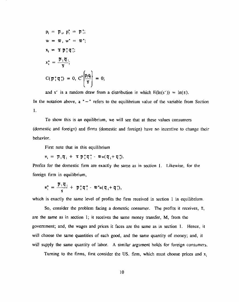
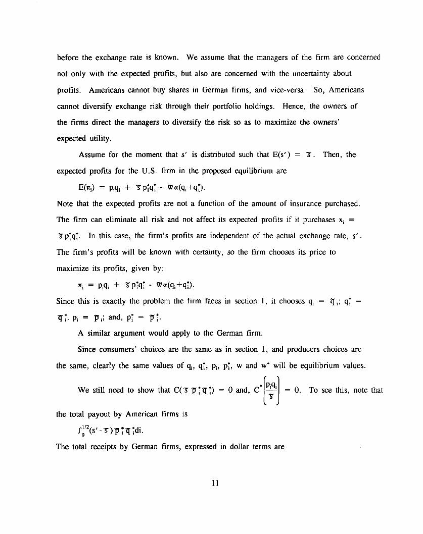
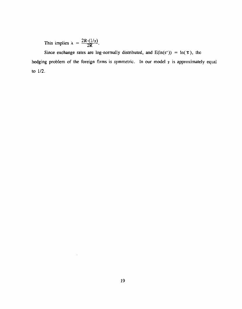
Since exchange rates are log-normally distributed, and E(ln(s’ )) = ln( x ), the
hedging problem of the foreign firms is symmetric. In our model 7 is approximately equal
to 1/2.
19
References
Betts, Caroline, and Michael B. Devereux, 1996, Exchange rate dynamics in a model ofpricing-to-market, University of British Columbia, working paper.
Chinn, Menzie D., and Richard A. Meese, 1995, Banking on currency forecasts: Howpredictable is change in money?, Journal of International Economics 38, 161-178.
Dombusch, Rudiger, 1976, Expectations and exchange rate dynamics, Journal of PoliticalEconomy 84, 1161-1176.
Dombusch, Rudiger, 1987, Exchange rates and prices, American Economic Review 77, 93-106.
Engel, Charles, 1992, On the foreign exchange risk premium in a general quilibriummodel, Journal of International Economics 32, 305-319.
Engel, Charles, 1993, Rd exchange rates and relative prices: An empiricalinvestigation, Journal of Monetary Economics 32, 35-50.
Engel, Charles, 1996, The forward discount anomaly and the risk premium: A survey ofrecent evidence, Journal of Empirical Economics 3, 123-192.
Engel, Charles, and John H. Rogers, 1996, How wide is the border?, American EconomicReview, forthcoming.
Flood, Robert P., and Andrew Rose, 1995, Fixing exchange rates: A virtual quest forfundamentis, Journal of Monetary Economics 36, 3-37.
Frankel, Jeffrey A., and Kenneth A. Froot, 1990, Chartists, fundamentalists, and thedemand for dollars, in Anthony Courakis and Mark Taylor, eds., Private behavior andgovernment policy in interdependent countries (Clarendon Press, Oxford).
Frankel, Jeffrey A., and Richard Meese, 1987, Are exchange rates excessively variable?,NBER Macrwonomics Annual 2, 117-162.
Friedman, Milton, 1953, The case for flexible exchange rates, in M. Friedman, Essays inpositive economics (University of Chicago Press, Chicago).
Grilli, Vittorio and Nouriel Roubini, 1992, Liquidity and exchange rates, Journal ofInternational Economics 32, 339-352.
Huang, Roger, 1981, The monetary approach to exchange rates in an efficient foreignexchange market: Tests based on volatility, Journal of Finance 36, 31-41.
Johnson, Harry G., 1972, The case for flexible exchange rates, in H.G. Johnson, Furtheressays in monetary monomics (Allen and Unwin, London).
20
King, Robert G.; Neil Wallace; and, Warren E. Weber, 1992, Nonfundamenti uncertainty andexchange rates, Journal of International Economics 32, 83-108.
Knetter, Michael, 1989, Price discrimination by U.S. and German exporters, American~nomic Review 79, 198-210.
Kroner, Kenneth F., and William D.volatility on international trade:
wmparisons of pricing-to-market behavior, American
hstrapes, 1993, The impact of exchange rateReducd form estimates using the GARCH-in-ma
model, ~oumal of International Money and Finanm 12, 298-318.
Krugman, Paul, 1987, Pricing to market when the exchange rate changes, in S. Amdt andJ.D. Richardson, eds,, R4-financial linkages among open economies (MIT Press,Cambridge, MA.).
MacDonald, Ronald, and Mark P, Taylor, 1994, The monetary model of the exchange rate:hng-run relationships, short-run dynamics and how to beat a random walk, Journal ofInternational Money and Finance 13, 276-290.
MLnkiw, N, Gregory, 1985, Small menu costs and large business cycles: A macroeconomicmodel of monopoly, Quarterly Journal of Economics 100, 529-539.
Manuelli, Rodolfo E. and James Peck, 1990, Exchange rate volatility in an equilibriumasset pricing model, International Economic Review 31, 559-574.
Mark, Nelson B., 1985, On time varying risk premia in the foreign exchange market: Aneconometric analysis, Journal of Monetary Economics 16, 3-18.
Mark, Nelson B., 1995, Exchange rates and fundamentals: Evidence on long-horizonpredictability, American Economic Review 85, 201-218,
Marston, Richard, 1990, Pricing to market in Japanese manufacturing, Journal ofInternational Economics 29, 217-236.
Meese, Richard, 1986, Tests for bubbles in exchange markets: A case for sparkling rates?,Journal of Political Economy 94, 345-373,
Meese, Richard, and Kenneth Rogoff, 1983a, Empirical exchange rate models of theseventies: Do they fit out of sample, Journal of International Economics 14, 3-24.
Meese, Richard, and Kenneth Rogoff, 1993b, The out-of-sample failure of exchange ratemodels: Sampling error or misspecification?, in J. Frenkel, ed., Exchange rates andinternational macroeconomics (University of Chicago Press, Chicago).
Rangan, Subramanian and Robert Z. Lawrence, 1993, The responses of U.S. firms to exchangerate fluctuations: Piercing the corporate veil, Brookings Papers on EconomicActivity 2, 341-379.
21
Tesar, Linda L. and Ingrid M. Werner, 1994, International equity transactions and U. S,portfolio choice, in Jeffrey A. Frankel, ed., The internationalization of equitymarkets (University of Chicago Press).