A Model of Self-fulfilling Exchange Rate Crisis With Sovereign Debts * Millan L. B. Mulraine † University of Toronto April 2007 Abstract The collapse of Argentina’s currency board provides further evidence that fiscal profli- gacy (whether financed by domestic money creation or foreign debt) is incompatible with the maintenance of any fixed exchange rate regime. In this paper we analyze a dynamic general equilibrium model with a mixture of fiscal deficits, stochastic endowment, and sovereign debts. It offers an environment in which a loss of confidence in the sustain- ability of the government’s fiscal position creates an environment for exchange rate crises. The evidence provided demonstrates that the Argentine government’s decision to abandon the peg in 2002 - following the default on its international debts, was a self-fulfilling out- come of agent’s expectations based on the underlying economic environment. Moreover, we also show that in an essentially identical economic framework - where the equilibrium probability of default is low, the optimal action for the government would be to maintain the fixed exchange rate and issue new debts to finance the fiscal deficit. Keywords: Debt crisis, Exchange rate crisis, Sovereign debts, Sunspots. JEL Classification: F34, F41, H63 * This paper forms part of my Ph.D. Economics thesis at the University of Toronto. I wish to thank Paul Masson for his supervision of this effort, and the many others who offered helpful suggestions and comments. All remaining errors are mine. † Corresponding address: Department of Economics, University of Toronto, 150 St. George Street, Toronto, ON M5S 3G7, Canada. Tel: 1 (416) 824 8069, Email: [email protected]
Transcript
A Model of Self-fulfilling Exchange Rate Crisis
With Sovereign Debts∗
Millan L. B. Mulraine†
University of Toronto
April 2007
Abstract
The collapse of Argentina’s currency board provides further evidence that fiscal profli-
gacy (whether financed by domestic money creation or foreign debt) is incompatible with
the maintenance of any fixed exchange rate regime. In this paper we analyze a dynamic
general equilibrium model with a mixture of fiscal deficits, stochastic endowment, and
sovereign debts. It offers an environment in which a loss of confidence in the sustain-
ability of the government’s fiscal position creates an environment for exchange rate crises.
The evidence provided demonstrates that the Argentine government’s decision to abandon
the peg in 2002 - following the default on its international debts, was a self-fulfilling out-
come of agent’s expectations based on the underlying economic environment. Moreover,
we also show that in an essentially identical economic framework - where the equilibrium
probability of default is low, the optimal action for the government would be to maintain
the fixed exchange rate and issue new debts to finance the fiscal deficit.
Keywords: Debt crisis, Exchange rate crisis, Sovereign debts, Sunspots.
JEL Classification: F34, F41, H63
∗This paper forms part of my Ph.D. Economics thesis at the University of Toronto. I wish to thank Paul
Masson for his supervision of this effort, and the many others who offered helpful suggestions and comments.
All remaining errors are mine.†Corresponding address: Department of Economics, University of Toronto, 150 St. George Street,
The first three generations of currency crisis models offer a rich literature for examining the
conditions under which a currency becomes susceptible to speculative attacks engendered by
the incompatibility between the exchange rate regime being pursued by the government and
the underlying macroeconomic fundamentals. In particular, this literature has been generally
successful in detailing both the timing and magnitude of these attacks and characterizing the
key fundamentals associated with them. However, despite the enormous insights provided by
these models they are unable to explain the three major1 episodes of international financial
crises that have occurred since the 1997 East Asian crisis. This inadequacy is principally
because the analysis provided by these models abstracts from one key component that has been
the hallmark of these three episodes of currency crises; namely the large and unsustainable
foreign-currency denominated sovereign debts.
In this paper we analyze a dynamic general equilibrium model with a mixture of persis-
tent fiscal deficits financed by foreign-currency denominated debt and stochastic exogenous
endowment. The paper offers an environment in which a sudden-stop in international finance
caused by a confidence crisis in the sustainability of the government’s fiscal position creates an
environment for an exchange rate crisis. As a consequence of the sudden-stop in the external
financing of the persistent fiscal deficits, the government is forced to default on its outstanding
debt payments and abandon the fixed exchange rate regime.
The objectives of the paper, therefore, are two-fold: firstly, the paper aims to characterize
the state-space in which a self-fulfilling debt crisis can arise in an environment in which there
are persistent fiscal deficits financed by foreign-currency denominated debt. In doing so, the
paper will also examine the conditions under which the government will choose to abandon the
fixed exchange rate regime after defaulting on its outstanding international debt obligations,
as opposed to implementing the requisite fiscal policy adjustments. Secondly, the paper will be
calibrated to match the stylized facts of the Argentine economy, and the proposed model will
then be simulated to explore its dynamic properties and to assess the welfare implications
of the decision of the Argentine government to abandon the currency board arrangement
following the default of 2002.1The three major crises are the Russian crisis, the Brazilian crisis, and the Argentine crisis.
2
The paper distinguishes itself from the previous generations of currency crisis models
and other related work in this area by providing an analysis of the welfare implications of
a government’s decision to default on its outstanding international debts and the post-crisis
decision regarding its policy choice of whether it should implement fiscal policy adjustments
in light of the incipient fiscal shortfall or abandon the fixed exchange rate regime. In doing
so the paper develops a general equilibrium model in which a debt crisis arising from the
self-fulfilling prophesy of agents results in a full-fledged currency crisis. The welfare analysis
conducted is aimed at offering some useful insights into the costs/benefits associated with a
government’s decision to default on its international debt obligations and the impact of that
decision on the welfare of agents in the economy.
The model developed here follows quite closely the experience of the collapse of the Ar-
gentine Convertibility Plan in which a cessation in the financing of the government’s fiscal
deficits by international investors due to their expectation on the probability of a government
default forced the Argentine government to default on its outstanding international sovereign
debt obligations in 2002 and subsequently abandon the Currency Board Arrangement (CBA).
While this model is based on the experience in a fixed exchange rate regime the model speci-
fication is general enough for consideration of other exchange rate regimes.
This paper is similar in scope to the work of Rebelo and Vegh (2002) which analyzes the
optimal time for a government to abandon its fixed exchange rate regime which has become
unsustainable when faced with exogenous fiscal shocks. The model to be analyzed extends the
insightful work of Cole and Kehoe (2000) in which a DGE model was developed to explain
the Mexican financial crisis of 1994-1995. This paper, however, differs from their work in a
number of key dimensions. Firstly, instead of characterizing the state-space within which a
debt crisis can occur2 a la Cole and Kehoe (2000), the paper focusses on the post-default
decision that a government must make when faced with a shortfall in its fiscal budget in the
absence of financing from international investors. Secondly, it provides a framework in which
the real depreciation of the exchange rate can be endogenously determined. Finally, the model
is driven by exogenous technological shocks to the production of the consumption good and2In their paper, the authors focus on characterizing the values of government debt and the debt’s maturity
structure under which a financial crisis can occur. They then go on to explore the policy options available to
the government when a financial crisis occurs.
3
shifts in the expectations of default on the debts by international investors - or sunspots.
In more recent work, Irwin (2004) attempts to explain the Argentine crisis by developing
a second generation currency crisis model that extends the work of the Obstfeld (1995), and
Drazen and Masson (1994), in which the policymaker has incomplete information about the
costs of devaluation and where unemployment is persistent. In their framework, the paper
shows that the persistence of unemployment causes the costs of maintaining the exchange rate
regime to be too high and forces the abandonment of the regime. Similarly, Komulaninen
(2004) considers the impact of foreign currency denominated debts in the context of the first
generation currency crisis model. In it he shows that international bond financing may not
necessarily delay the timing of these crises since the lower money demand due to the higher
risk premium may bring the timing of the crisis forward. He, however, concludes that if the
country’s indebtedness is low to moderate, bond financing will invariably delay the timing of
the crisis.
While the analysis provided in these papers is useful, they do not take account of the fact
that the currency crisis in Argentina was induced by the cessation of external financing of the
government’s fiscal deficits. More importantly, they do not consider the welfare implications
of the policy choices of the government, and as such they are unable to make judgements on
the optimality of the decision of the Argentine government to abandon the currency board
arrangement in favor of a free float following the default of 2002. For more detailed analysis
of the events leading up to the Argentine currency crisis, see Mulraine (2004).
The remainder of the paper is divided into six sections. In Section 2 of this paper the
two-period DGE model is presented, with its dynamic properties discussed in Section 3. In
Section 4 we explore the rational expectations equilibrium of the model. While in Section 5
the model will be simulated to provide insights into the decision of the Argentine government
to default on its external debts and to abandon the exchange rate upon defaulting. The paper
then concludes in Section 6.
2 The Benchmark Model
Consider a two-period dynamic general equilibrium small open economy model in which there
exist three types of economic agents. A representative consumer who makes consumption
4
decisions, a government (or public sector) that is responsible for all monetary and fiscal policy
decisions in this stylized economy, and a representative risk-neutral international investor who
purchases bonds issued by the government on the international capital market.
2.1 The Representative Consumer
This small open economy is populated by a large number of identical consumers of mass one
who live for two periods. Each period the representative consumer receives an exogenous
endowment of the consumption good yt, which is divided between consumption and financial
asset holdings - in the form of money. The discounted utility function for these agents can be
expressed as:
maxct,mt+1
u(ct) + βEtct+1, 0 < β < 1 (1)
where ct is the consumption level of the composite consumer good and β is assumed to be
the constant discount factor for agents in the economy. The first period utility functional
u(.) is assumed to be concave, continuously differentiable and monotonically increasing in its
argument. Following Drazen (1998), we assume that the representative consumer has linear
preferences in the second period3.
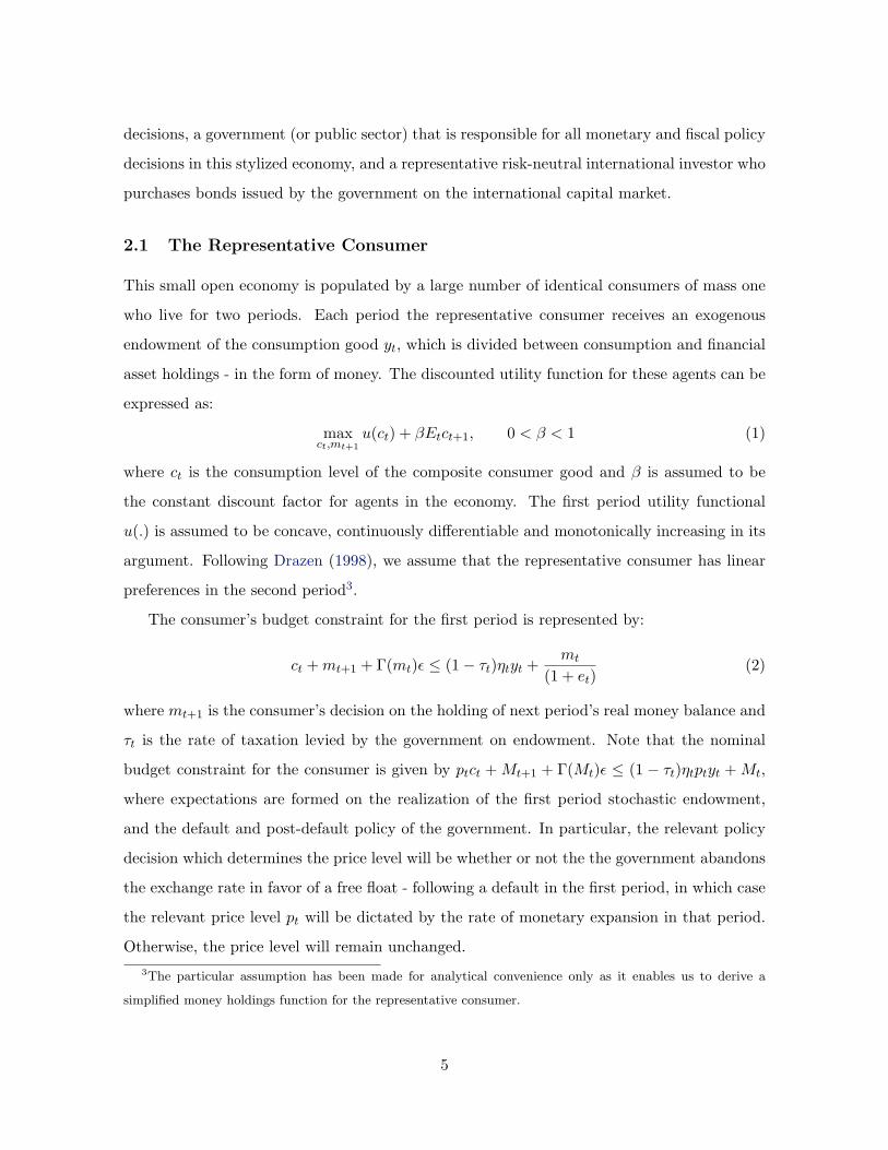
The consumer’s budget constraint for the first period is represented by:
ct + mt+1 + Γ(mt)ε ≤ (1− τt)ηtyt +mt
(1 + et)(2)
where mt+1 is the consumer’s decision on the holding of next period’s real money balance and
τt is the rate of taxation levied by the government on endowment. Note that the nominal
budget constraint for the consumer is given by ptct + Mt+1 + Γ(Mt)ε ≤ (1 − τt)ηtptyt + Mt,
where expectations are formed on the realization of the first period stochastic endowment,
and the default and post-default policy of the government. In particular, the relevant policy
decision which determines the price level will be whether or not the the government abandons
the exchange rate in favor of a free float - following a default in the first period, in which case
the relevant price level pt will be dictated by the rate of monetary expansion in that period.
Otherwise, the price level will remain unchanged.3The particular assumption has been made for analytical convenience only as it enables us to derive a
simplified money holdings function for the representative consumer.
5
Moreover, with the assumption of the law of one price, such that pt = Stp∗t where St
represents the nominal exchange rate4, the variable et = St−St−1
St−1will depict both the inflation
rate (or rate of domestic nominal money creation) and the rate of depreciation of the domestic
currency, following a float. Note that the opening stock of real money holdings, Mtpt
, can be
simplified by multiplying by pt−1
pt−1to get the expression mt
1+etshown in Eq. 2, where et = pt−pt−1
pt−1,
mt = Mtpt−1
, and mt+1 = Mt+1
pt. Thus, it becomes evident from this equation that real nominal
balances held by agents are eroded by inflation given by et.
The variable yt represents a first period exogenous stochastic endowment that is drawn
from a continuous distribution, with density function given by fy(·) about its mean of 1, and
has a cumulative distribution function Fy(·). In the second period, however, the exogenous
endowment yt+1 is assumed to be non-stochastic and is set equal to its expected value of unity.
Following Bulow and Rogoff (1989), (1 − ηt) is a multiplicative output loss which depends
on whether or not the government defaults on its outstanding debts. It reflects the fraction
of output loss each period following a default by the government as a result of the direct
sanctions imposed by the holders of government debts.
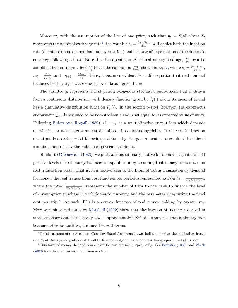
Similar to Greenwood (1983), we posit a transactionary motive for domestic agents to hold
positive levels of real money balances in equilibrium by assuming that money economizes on
real transaction costs. That is, in a motive akin to the Baumol-Tobin transactionary demand
for money, the real transactions cost function per period is represented as Γ(mt)ε = 1mt/(1+et)
ε,
where the ratio[
1mt/(1+et)
]represents the number of trips to the bank to finance the level
of consumption purchase ct with domestic currency, and the parameter ε capturing the fixed
cost per trip.5 As such, Γ(·) is a convex function of real money holding by agents, mt.
Moreover, since estimates by Marshall (1992) show that the fraction of income absorbed in
transactionary costs is relatively low - approximately 0.8% of output, the transactionary cost
is assumed to be positive, but small in real terms.4To take account of the Argentine Currency Board Arrangement we shall assume that the nominal exchange
rate St at the beginning of period 1 will be fixed at unity and normalize the foreign price level p∗t to one.5This form of money demand was chosen for convenience purpose only. See Feenstra (1986) and Walsh
(2003) for a further discussion of these models.
6
2.2 The Public Sector
The public sector issues money and produces the requisite level of nonproductive services
g each period. In light of the fiscal deficit facing the fiscal authority in the first period,
a decision is made on the amount of sovereign one-period zero-coupon bonds qtbt+1 to be
issued on the international capital market, where qt represents the price of these one-period
discounted bonds with face value bt+1 - specifying the amount to be repaid in period t + 1.
Moreover, since the government cannot commit ex-ante to full repayment of the outstanding
debts bt6 coming due in the first period, it must also make a strategic decision on whether
it should default on the current payments that have become due. The default decision is
captured by the indicator function Dt ∈ 0, 1, with 0 meaning a non-payment or full default
on the outstanding debt payments due and 1 indicating a full repayment. Note that if the
government defaults on its outstanding international debts in the first period the economy
faces a punishment factor 0 < 1− ηt < 1 on its exogenous endowment which captures events
such as loss of market access (embargo on trade) or tariffs imposed on it exports in both
periods. Moreover, we shall also assume that the government cannot default on its second
period debts bt+1.
The public sector is comprised of a benevolent government which considers the utility
function of the representative consumer as its own, and therefore maximizes the utility func-
tion of these agents given by Eq. 1 with respect to its choice of new bond holdings, bt+1 -
given its price qt, subject to the following fiscal budgetary constraints:
g + Dtbt ≤ ∆(τt)ηtyt + qtbt+1 + mt+1 −mt
(1 + et)(3)
Note that provided that the government has not defaulted previously, it will have access
to unlimited bond financing resources which it can obtain through the issuance of one-period
zero-coupon bonds bt+1 on the international capital market at a price qt = 11+ict
, with the
country-specific rate of interest given by ict = i∗ + φct(π1, bt), where i∗ is the constant world
interest rate, and φct(π1, bt) represents a country-specific spread charged by foreign investors for
holding the unsecured government bonds. φct(π1, bt) is an increasing function of the probability
6As part of the state of nature for the economy at the beginning of period 1, the opening stock of debt (bt)
- along with the opening stock of money (mt) - will be exogenously determined. However, they will collectively
capture the history of events for the Argentine economy.
7
of default π1, and a non-decreasing function of the bonds issued bt. In the absence of this
external avenue for financing its deficit - the loss of which occurs when the government has
defaulted on its outstanding debts - the government must finance its deficits by either money
creation or taxes.
Here, the level of additional real resources that is generated from seigniorage mt+1− mt(1+et)
(where Mt+1 = (1+et)Mt), depending on the nature of the exchange rate regime being pursued
by the government is given by the expression(
et1+et
)mt
7. That is, if the post-default policy
choice made by the government is to abandon the exchange rate regime in favor of a float, then
the government has the ability to garner additional real revenue by expanding the nominal
money supply such that M st+1 = (1+ξt)M s
t , where ξt represents the rate of nominal monetary
expansion. The increase in the nominal money supply raises current prices to ensure market
clearing of the real money supply. The resultant inflation along with the assumption of the
law of one price, therefore, causes a depreciation of the domestic currency by an amount
equivalent to the rate of price inflation, such that et = ξt. In the second period, however,
government loses its ability to use seigniorage as the end of the period holdings of real money
will be zero, consequently, inflation in that period will be zero.8
The function ∆(τt) represents the effective tax rate imposed by government on endowment.
It becomes relevant in the case where the government pursues a “tax policy” regime following
a default on its outstanding debts in the first period - indicated by a τ superscript. Following
Aizenman et al. (2000) we assume that adjusting the tax level in the first period beyond its
fixed initial level τ incurs additional cost to the fiscal authority. These costs may reflect the
inherent inefficiency in the tax collection system and thus they capture the distortions caused
by changes in the rate of taxation, alternatively, they can be seen as the additional collection
costs incurred by the government. As such, we specify a simplified function by assuming a
fixed portion φ of the tax collected is lost, in which case ∆(τt) = (1− φ)τ τt .
7Recall that the real seigniorage revenue given byMt+1
pt− Mt
ptcan be simplified by multiplying the second
expression bypt−1pt−1
to get mt+1 −mtmt
(1+et), where 1 + et = pt
pt−18Note that in the second period the government assumes the monetary liabilities of the previous period.
However, since this is financed by further taxation there will be no net change in real resources available to
agents in the economy as a result of this action.
8
2.3 The International Investor
There exist a large number of risk-neutral international investors with access to unlimited
funds - operating in a perfectly competitive international capital market. The representative
international investor holds a diversified portfolio of assets of which the sovereign debts of
this small open economy is a negligible part. As such, the combination of investment risk
neutrality of this agent and risk idiosyncracy of the sovereign bonds held ensures that the
problem of the international investor collapses to an arbitrage condition which equalizes the
expected gross interest rate earned from investing in one unit of the risky sovereign bonds
to the risk-free rate of return prevailing on the international capital market. That is, the
international investor will invest in domestic risky sovereign bonds up to the point where the
expected return from these bonds (1− π1)(1 + ict) becomes equal to the risk-free return from
other international bonds (1 + i∗t ), such that (1− π1)(1 + ict) = (1 + i∗t ). This implies that for
the international investor β∗Et(1+ ict) = 1, where 1β∗ represents the rate of time preference for
the international investor and π1 denotes the probability of a default by the fiscal authority
on its international debts.
From this condition it becomes apparent that the implicit country-specific spread de-
manded by international investors on their holdings of the international bond is an increasing
function of the probability of default. More specifically, we can see that as the probability
of default approaches 1 the country-specific spread approaches infinity, and conversely as the
default probability approaches zero the expected rate approaches the risk-free world interest
rate. That is, limπ1→1 ict+1 → ∞, and similarly limπ1→0 ict+1 → i∗t . Given the assumption of
unlimited financial resources available to the international investor and the collapse of the
problem of the international investor to the arbitrage condition outlined above, we can there-
fore remove the problem of this agent from further consideration, and instead focus on the
formation of the probability of default.
2.4 Timing of Events
In this framework the timing of events in the first period is particularly important since
it dictates the information set available to each agent at the time the requisite optimizing
decisions are being made by these agents. More specifically, at each point when these opti-
9
mizing decisions are being taken, all previous decisions (made by other agents) will be known.
Accordingly, the timing of events goes as follows:
1. The international investors set out a financial strategy regarding the purchasing of
government bonds, given their expectation on the probability of default π1 following the
realization of the sunspot variable9 π, and their current holdings of government bonds bt;
2. The consumer chooses the level of consumption ct, and consequently the ex-ante level
of money holdings mt+1 for the next period.
3. Given the price schedule for government bonds on the international capital market
qt(π1, bt) and the financing requirement of the government qtbt+1, the value of the second
period debt bt+1 will be determined;
4. The exogenous endowment yt is realized and the full state of nature Ωt(bt,mt, yt, π)
becomes known;
5. Given this state of nature, the government then chooses whether or not it should default
on its outstanding debt bt;
6. If the government defaults on its debt10, it then determines the post-default policy
decision of whether to abandon the exchange rate regime in favor of a free-float or to maintain
the exchange rate regime and implement tax reform; and
7. The government’s decision determines the ex-post money holding mπt+1
11, based on
the default and post-default decision of the government and the level of the first period
consumption ct.
8. Given the absence of uncertainty in the second period, the equilibrium actions of all
agents will be assumed to occur simultaneously.
Furthermore, we shall assume that a technology exists to enforce payment of the outstand-
ing debts bt+1 that have become due in the second period. Finally, given that the terminal
value of the money holdings and the outstanding debt stock12 must be equal to zero at the
end of period two, the tax rate invariably adjusts in this period to ensure fiscal solvency under
all policy regime - in which case we restrict the analysis to cases where τπt+1 < 1.
9This sunspot variable is assumed to be independently and uniformly distributed on the unit interval, such
that π ∈ [0, 1], and occurs as a shock to the expectations of international investors.10At the time that the government default decision arises its stock of outstanding debt will be bt and bt+1.11Where π ∈ n, s, τ depending on the policy decision of the government.12Note that there will be no new lending by the international investors to the government in that period.
10
Following Cole and Kehoe (2000), we shall assume that in the first period agents observed
an exogenous sunspot variable π, assumed to be uniformly distributed on the interval [0,
1]. In equilibrium, if the sunspot variable π ≤ π1, upon seeing this signal agents rationally
predict a default by the government on its outstanding debts. If so, agents will be unwilling
to pay a positive price for any new debt offered by the government. In which case the cost
of issuing new bonds to retire the old debts becomes prohibitively large for the government,
thus triggering a debt crisis. Conversely, for sunspot variable π > π1, international investors
rationally expect the government to repay in full the outstanding debts, and thus they will
be willing to make new loans to the government to finance it deficits. Since π is uniformly
distributed on the unit interval, we will have that π1 is both the crucial value of π and the
probability of default (that is, π ≤ π1).
3 Equilibrium Dynamics
Given this framework, we can now focus on the sequence of events outlined above. To solve the
problem at hand we shall revert to a framework in which we solve the problems of the agents
at the beginning of a period before which there has never been any default and expectations
are formed on the current period’s default and post-default decisions of the government.
3.1 The consumer’s optimal decisions
The consumer’s decision in the first period is affected by her expectations on the govern-
ment’s default and subsequent post-default decisions in that period. Since a default on the
outstanding debt payment will invariably mean that the government must balance its fiscal
budget by either abandoning the exchange rate regime or adjusting the tax rate, the consumer
must form expectations on these occurrences and take account of them in her problem. To
this end, the budget constraints given below are for the no-default (denoted by n), default
with floating exchange rate (denoted by s), and default with tax adjustment (denoted by τ),
respectively. Let us assume that the representative consumer expects the government will
default with probability π1, and upon defaulting abandons the exchange rate with probability
π2. As such, the consumer’s maximization problem at the beginning of the first period in
which she chooses the consumption level for the current period and the ex-ante level of next
11
period’s money holdings, given by ct and mt+1, respectively - where expectations are formed
over the respective government action and the stochastic exogenous endowment for the first
period yt - can be represented as:
maxct,mt+1
c1−γt − 11− γ
+ βEtct+1, 0 < β < 1 (4)
subject to
ct + mt+1 +[ 1mt/(1 + et)
]ε ≤ (1− τt)ηtyt +
[ mt
(1 + et)
](5)
ct+1 +1
mt+1ε ≤ (1− τt+1)ηt+1yt+1 + mt+1
Here the representative consumer maximizes expected utility subject to the three possible
equilibrium outcomes based on the default and post-default decisions of the government. The
variables cnt+1, c
τt+1 and cs
t+1 are the ex-post state-contingent second period consumption level
under a no-default, default and tax, and a default and float equilibrium, respectively. That
is, the consumer chooses the levels of consumption ct, and ex-ante money holding mt+1, with
the ex-post value of the asset portfolio mπt+1 where π ∈ n, s, τ, being determined by the
respective actions of the government and the choice of mt+1 in the first period.
The optimal equilibrium equations for first period consumption, expected second period
consumption and the ex-ante money holdings, respectively, can be restated as:
ct = Et(1− τt)ηtyt + Et
[ mt
1 + et
]− Et
[1 + et
mtε]− mt+1 (6)
Etct+1 = (1− π1)[(1− τn
t+1)yt+1 + mnt+1 −
1mn
t+1
ε]
+ π1(1− π2)[(1− τ τ
t+1)ηt+1yt+1 + mτt+1 −
1mτ
t+1
ε]
+ π1π2
[(1− τ s
t+1)ηt+1yt+1 + mst+1 −
1ms
t+1
ε]
(7)
and
mt+1 =[ βcγ
t
1− βcγt
ε] 1
2 (8)
Here, the superscripts n, s and τ on the ex-post variables capture the no-default, default
and float, and default and tax regimes, respectively, resulting from the first period actions of
the government. An important consideration for the analysis to follow will be the analytical
12
expressions for the ex-post equilibrium variables under the three possible policy choices of
the government. Recall that the consumer chooses the optimal level of consumption ct and
the ex-ante money holdings mt+1 in the first period prior to the revelation of the state of
nature. However, following the decision of the government in the first period, the consumer
consumes the optimal level of consumption regardless of the regime pursued and allows her
money holding to adjust ex-post to balance her budget. In the second period the agent will
consume the sum of her endowment (net of taxes) for that period and the money holdings
brought forward from the previous period, less the transaction cost.
As outlined above, in the first period the representative consumer-producer chooses the
unique13 ex-ante optimal level of consumption and lets the money holdings that are carried
forward into the second period depend on the government’s policy decision.
At the end of the first period when all uncertainties are resolved and the policy of the
government has been established, we can derive the level of capital stock associated with each
decision of the government, and consequently the implied levels of consumption in the second
period. More specifically, in an environment where the stochastic endowment is given by yt
and the government does not default on its debt obligations (in which case price remains
unchanged), the values for next period’s money stock and consumption become:
mnt+1 = (1− τ)yt + mt −
1mt
ε− ct (9)
and
cnt+1 = (1− τn
t+1)ηt+1yt+1 + mnt+1 −
1mn
t+1
ε, where ηt+1 = 1 (10)
If instead, the government defaults on its outstanding debt payment and decides to maintain
the exchange rate regime by implementing tax adjustments, the value for the next period’s
money holdings and consumption will be:
mτt+1 = (1− τ τ
t )ηtyt + mt −1
mtε− ct (11)
and
cτt+1 = (1− τ τ
t+1)ηt+1yt+1 + mτt+1 −
1mτ
t+1
ε (12)
13This consumption level is considered unique in the sense that the level of consumption by agent remains
invariant to the policy regime subsequently pursued by the government.
13
Finally, in a scenario where the government defaults on its debt payment and decides to
abandon the exchange rate regime while using seigniorage revenue to finance the budgetary
gap, the value for the next period’s money holding and consumption then become:
mst+1 = (1− τ)ηtyt +
[ mt
1 + et
]−
[(1 + et)mt
ε]− ct (13)
cst+1 = (1− τ s
t+1)ηt+1yt+1 + mst+1 −
1ms
t+1
ε (14)
From Eq. 6 - 8 above it becomes evident that the consumption level ct, and consequently the
ex-ante level of money holding mπt+1 depend explicitly on the ex-ante probabilities assigned
by agents to the policy choices of the government. This observation is particularly important
since it is the underpinning of the self-fulfilling nature of the model.
3.2 The government’s optimal decisions
Recall that the government’s decision on the optimal amount of new bonds to issue occurs
before the realization of the productivity innovation - thus there will still remain uncertainty
about the state of nature when the government makes its first move. This uncertainty, there-
fore, requires that the government’s decision on the optimal amount of bonds to issue be
contingent on its expectations of the realization of the productivity innovation in that period.
Moreover, given our assumption of risk neutrality and unlimited funds on the part of the
representative international investors, the government will be able to issue new bonds in the
first period equivalent to qtbt+1 to balance its budget.
By the time the government makes its default decision in the first period, the state of
nature Ωt(bt,mt, yt, πt) will be fully revealed. As a result, the problem for the government
when it makes the default decision can be described as:
V πg (π1, π2) = max
π
c1−γt − 11− γ
+ βcπt+1 (15)
subject to
g + bt ≤ τyt + qtbt+1 (16)
g ≤ (1− φ)τ τt ηtyt + qtbt+1 (17)
g ≤ τηtyt + qtbt+1 +( et
1 + et
)mt (18)
14
From these equations we can obtain the equilibrating values14 for qtbt+1, τ τt , and et that
will be required to balance the government’s budget in the first period in the no-default, the
default and tax, and the default and float equilibrium, respectively. In the case of a float, the
government uses seigniorage revenue given by(
et1+et
)mt
15, thus allowing the exchange rate to
depreciate endogenously to balance its budget. Similarly, we can also obtain the second period
equilibrating values for τnt+1, τ τ
t+1 and τ st+1 under the three policy regimes of the government.
Having fully characterized the optimal decisions of the representative consumer and the
behavior of the government, we are now interested in determining the regions of the state
space in the stochastic endowment and debt stock, yt, bt - for a given level of opening stock
of money holding mt - in which the default and post-default decisions of the government lie.
More specifically we are interested in finding the range in the state space for which it will
be optimal for the government to (i) default on its outstanding debts, and in so doing to (ii)
abandon the exchange rate regime. Given that the optimal levels of consumption in both
periods are functions of the underlying ex-ante probabilities assigned to the respective policy
options of the government, the above problem for the government implies that the authorities
will choose to default on the outstanding debt payments that have become due this period
iff :
V dg (π1, π2) ≥ V n
g (π1, π2) (19)
Where V dg (π1, π2) = maxV s
g (π1, π2), V τg (π1, π2). That is, the government will default ex-
post if the discounted value of defaulting exceeds the expected discounted value of not de-
faulting. If the government defaults then it must decide on whether or not it should adjust
taxes or float the exchange rate to balance its fiscal budget. Therefore, the authority will opt14Note that at the end of the second period we must have that mt+2 = 0 and bt+2 = 0, thus meaning that
taxes τπt+1 must adjust to ensure fiscal solvency. For a complete list of the ex-post equilibrating values for
the international borrowing qtbt+1, the tax rate ττt , and the rate of depreciation et in the first period for the
government under the no-default, default and tax, and default and float, respectively, and their associated
second period tax rates τπt+1 see Appendix 7.1.
15This expression for the seigniorage revenue emerges from the government’s budget constraint. In nominal
terms, the government’s budget constraint is given by ptg ≤ τηtptyt +qtptbt+1 +Mt+1−Mt, where the nominal
seigniorage revenue is Mt+1−Mt, after substituting Mt+1 = (1+et)Mt and dividing by pt we get the expression
for the real seigniorage revenue obtained by the government.
15
to abandon the fixed exchange rate regime iff :
V sg (π1, π2) ≥ V τ
g (π1, π2) (20)
that is, if the discounted expected value of floating after a default exceeds that of implementing
tax reform.
3.3 Value function properties
The analysis provided so far has focussed exclusively on outlining the decision rules that
govern the behavior of a benevolent government in determining its default and post-default
decisions. The analytical form of the ex-post value functions for the no-default policy options
for the government is given by:
V πg =
c1−γt − 11− γ
+ β[(1− τπ
t+1)I(ηt+1)yt+1 + mπt+1 −
ε
mπt+1
], where π ∈ (n, τ, s) (21)
and I(ηt) is an indicator function such that
I(ηt) =
1 if π = n;
ηt if π = τ ;
ηt if π = s.
For a complete list of the ex-post equilibrating values for the international borrowing qtbt+1,
the tax rate τ τt , and the rate of depreciation et in the first period for the government under the
no-default, default and tax, and default and float, respectively, and their associated second
period tax rates τπt+1 see Appendix 7.1. This then takes us to the next step of the analysis
- which is to discuss some properties of the government’s value function with respect to the
state variables and the underlying ex-ante probabilities. This we shall now do in the form of
a few theorems.
Theorem 3.1. The discounted value of not defaulting each period, V ng (π1, π2), is inversely
related to the ex-ante expected probability of a default, π1.
Proof. See Appendix 7.2.
The rationale for this theorem comes from the fact that higher ex-ante expectation of the
probability of default on the part of agents increases the country-specific spread φ(π1, bt), and
16
hence the country-specific interest rate ict charged on any new borrowing by the government.
This higher country-specific interest rate lowers the price for government bonds qt. Given that
for any given initial state characterized by Ωt(bt,mt, yt, πt), the sacrifice required in period
two to repay the accumulated debt bt+1 - resulting from higher taxation in that period -
will be an increasing function of ex-ante probability of default π1. It therefore implies that
the discounted value of not defaulting decreases with the ex-ante expected probability of a
default, that is dV ng (π1,π2)
dπ1< 0.
This observation is particularly important since it underpins the self-fulfilling nature of
the model being considered. That is, when agents expect the government to default with
certainty by setting π1 = 1, the costs of any new borrowing bt+1 becomes infinitely large,
and its price qt approaches zero. This makes it impossible for the government to repay its
outstanding debts since it will be unable to issue new bonds, making the prophesy of the
government’s default on outstanding debts self-fulfilling.
Theorem 3.2. The ex-ante expected probability of a default on the outstanding debts by the
government in a rational expectations, sunspot equilibrium, π116, will be an increasing function
of the debt stock, bt.
Proof. See Appendix 7.3
Essentially, this claim asserts that the greater the outstanding debt stock of the govern-
ment, the greater will be the amount of new bond issue required to finance the budget deficit
in that period, and consequently the greater will be the probability of a default. More pre-
cisely, as the debt stock moves toward the natural borrowing limit b17 the ex-ante probability
of default on these outstanding debts approaches unity.16The notion of a rational expectations, sunspot equilibrium follows the discussion outlined by Jeanne (1997)
and Jeanne and Masson (2000).17Here the natural borrowing limit (or debt ceiling) is defined as the maximal finite value of debt that the
government can afford to repay in all possible states if all revenues are devoted entirely to debt financing. See
Eaton and Gersovitz (1981) for further discussion on the debt ceiling.
17
4 Rational expectations, Sunspot Equilibrium
A rational expectations, sunspot equilibrium, therefore, in this framework is a one-to-one
mapping between the ex-ante probability assigned by agents to the respective government
actions (the default and post-default decisions) and the actual probability of the actions
taken by the government. As such, given the rationality of agents in the model the ex-ante
probability of default π1 and the ex-ante probability of a float π2 (following any default), will
be equal to the probability that the utility to the government of the requisite policy choice
exceeds that of the alternative option(s) available.
For example, we can derive the actual probability of a float π2 following a default, which
is given by:
π2 = Pr[V sg (π1, π2) ≥ V τ
g (π1, π2)] (22)
Which simplifies to:
π2 = Pr[cst+1 − cτ
t+1 > 0]
= Pr[( φ
1− φ
)(g − qtbt+1)−
( g − τηtyt − qtbt+1
mt + τηtyt + qtbt+1 − g
)( ε
mt
)> 0
](23)
Here, the actual probability of a float following a default on the outstanding debt will be
equal to the probability that the welfare loss to consumers in the form of higher transaction
cost - given by the second term in the bracket - is less than the welfare cost of higher taxation
expressed by the first term. As such, it becomes evident that the probability of a currency crisis
occurring following a debt crisis is strictly increasing with the size of the opening monetary
base, as the value of the real seigniorage revenue generated from this policy option increases
with the size of the opening monetary stock. The equilibrium probability of a float arising
from the above equation is an explicit function of the underlying economic fundamentals and
the stochastic process.
In a similar fashion, the equilibrium probability of the government defaulting on its out-
standing debts, given the state of nature must be equal to the probability that the discounted
welfare of defaulting is greater than that of not defaulting. Here, the expected welfare of a de-
fault will be directly related to the ex-ante probability assigned by agents on the post-default
actions of the government. That is, the probability of a default by the government, π1 on its
18
outstanding debts is given by:
π1 = Pr[V dg (π1, π2) ≥ V n
g (π1, π2)] (24)
Where V dg (π1, π2) and V n
g (π1, π2) are the value function for the government under default
and no-default, respectively. Given that consumption in the first period does not depend on
the policy decision of the government, the probability of a default in the first period then
simplifies to:
π1 = Pr[(1− π2)cτ
t+1 + π2cst+1 − cn
t+1 > 0]
(25)
Such that:
π1 = Pr[π2[(1− τ s
t+1)ηt+1yt+1 + mst+1 −
ε
mst+1
] + (1− π2)[(1− τ τt+1)ηt+1yt+1 + mτ
t+1 − ...
ε
mτt+1
] + (1− τnt+1)yt+1 + mn
t+1 −ε
mnt+1
> 0]
(26)
Given the complexity of the expression, this equation does not have a closed-form analyt-
ical solution, so in order to provide further insights into the properties of this model we shall
apply numerical methods. This approach will also provide us with the opportunity to assess
the implication of the model for the decision of the Argentine government to default on its
outstanding debts in 2002 and subsequently to abandon the fixed exchange rate regime.
5 Quantitative Assessment
5.1 Parameter Calibration
In this section we apply numerical methods to the model outlined above to ascertain the
relevant equilibrium probabilities, and to assess the welfare implications of the ex-ante proba-
bilities assigned by agents to the respective government’s actions. To do this, we shall calibrate
the stylized model as closely as possible to the Argentine economy at the end of 200118 - the
year before the Argentine government defaulted on its international debt. These calibrated
values were obtained by matching the empirical facts on the Argentine economy. Following
IMF (2003) the tax rate τ was set equal to 23.7% to reflect the total revenue of the Argentine
government in 2001 and the fixed amount of annual government spending g equal to 25%18See Table 1 for a summary of the parameter values used in the simulation.
19
of the expected endowment in the first period, which is equivalent to the ratio of primary
government expenditure to GDP in 2001. This takes into account the fact that at the end
of 2001 the Consolidated Government Account in Argentina had a primary deficit of 1.3% of
GDP. The stock of debt19 that came due in the first period was set at 4.6% of GDP, equivalent
to the total debt servicing by the Argentine government in 2001. Thus, the financing gap for
this period, which is the amount required to be raised on the international capital market,
was set at 5.9% of GDP.
We set the value of the opening stock of money holdings in the model to 12% of GDP to
reflect Argentina’s monetary base (measured by M2) at the end of 2001.20 Following Aguiar
and Gopinath (2004), we set the risk-free world interest rate at 4% and the endowment loss
or default penalty (1 − η) equal to 8% of output21. We set the constant discount rate β to
0.96 and follow the calibrated value of Yue (2005) by setting the coefficient of relative risk
aversion γ to 2. Using the functional form advocated by Aizenman et al. (2000), the tax
revenue loss φ resulting from implementing a tax policy adjustment was set equal to 1.5%.
Given the parameterization described above, the only remaining parameter to be determined
in this model will be ε - the fixed transaction cost. This parameter is particularly important
since it determines (to a large extent) the money holding decision of agents to the exogenous
process considered. Following Marshall (1992) we set ε equal to 0.0014 to obtain transaction
cost of 1% of GDP in the first period. To close the model, the experiment was conducted on
stochastic endowment yt in the first period, such that yt ∈ [0.65, 1.35], reflecting the vagaries
of annual per capita growth in Argentina22 - which moved from a high of +11% in 1991 to
a low of -15% in 2002, following the default23. Finally, the model was simulated with the19Given the two-periods dimension of the model, the debt considered in the simulation is the amount be-
coming due for the period. Note that a period in this framework was arbitrarily set to be equivalent to one
year. As such, the analysis conducted in the simulation exercises abstracts from the stock of debt in Argentina
which at the time of the crisis was close to 65% of GDP.20This value was obtained from Cline (2003).21In the case of Argentina the default penalty (or more precisely, the output loss) resulted from, inter alia, the
withdrawal of a number of international financial institutions - such as The Bank of Nova Scotia’s Scotiabank
Quilmes subsidiary in 2002 - and the higher costs of financial intermediation ensuing from the distress in the
Argentine financial sector following the default.22Note that the stochastic endowment spread was set arbitrarily wide to enhance the geniality of the results.23The Currency Board Arrangement was introduced in Argentina in April 1991 and abandoned in January
20
state-space grid being set to 20 possible outcomes.
5.2 Simulation Results
In Figure 1 we display the first period consumption level of the representative consumer in
the model, as functions of the ex-ante probability of the default and post-default policies
of the government. This consumer choice variable is an important gauge of the consumer’s
first period welfare in this stylized economy since they indicate how the perception of agents
toward the respective government actions affects their decision. In this framework, the agent’s
perception is reflected by the ex-ante probabilities assigned to the respective government
actions. Recall that the first period consumption level will be identical across all three policy
regimes, and as a consequence, it becomes a useful measure of how agents alter their decisions
based on what they perceive the government will do.
It becomes evident from the graph in Figure 1 that the first period consumption level for
the representative consumer is maximized in an environment where agents assign a value of
zero to the probability of the government defaulting on its outstanding debt. Conversely, the
representative consumer’s first period consumption level is at its lowest level when they assign
a high probability to the government defaulting on the outstanding debt with a concomitant
low ex-ante probability of a float, following a default by the government. That is, when the
probability combination of (π1, π2) is equal to (1,0).
The contrasting outcomes of these two polar cases highlight the fact that in an essen-
tially identical economic environment agents’ first period welfare will be higher if they expect
the government to repay its outstanding debt at the end of the period - compared to the
alternative of a default. This outcome emerges from the fact that the belief of a default
by government will result in all costs being passed on to them as the government will be
faced with higher borrowing costs on the international capital market - resulting from the
country-specific spread. This implies that for the Argentine economy, the pervasive view that
the government was about to default on its outstanding debts resulted in a sub-optimal out-
come for the Argentine people, in the sense that it resulted in lower first period consumption,
compared to an environment where the economic fundamentals would have dictated the ex-
2002. Between 1998 and 2002 real GDP per capital fell by as much as 25%.
21
pectation of agents to be one where they believe the government will repay its outstanding
debt.
On the other hand, the evidence provided by the model shows that the representative
agent’s first period consumption is higher when the government is expected to choose to
abandon the fixed exchange rate regime following a default, compared to the alternative of
pursuing a fiscal adjustment policy. The intuition for this is quite clear. Since agents can
only smooth consumption inter-temporally by holding money, in the event that they believe
that the government will pursue an expansionary monetary policy following a default, the
substitution effect will engender agents to increase their consumption in the first period to
avoid the confiscation of their money holdings by inflation. But there is also an income
effect that works in the opposite direction. In this case, the expectation of being poorer will
encourage the reduction in consumption and the accumulation of assets in the form of money.
Note, however, that the dominance of the substitution effect over the income effect is reversed
in the case where agents expect the government to pursue a fiscal agenda following the default.
In fact, in the case where agents expect the government to pursue fiscal policy following the
default there will be no substitution effect since inflation will be zero.
The unique equilibrium probability of a float, following a sovereign debt default, is equal
to 84%. That is, following a default, the probability of the government abandoning the fixed
exchange rate for a free float was very high. Regardless of the state of nature, there is a
high chance that the government will pursue an expansionary monetary policy to off-set any
budgetary deficit that may arise from the loss of access to the international capital market -
following a default on the international debt. In essence, this outcome mirrors the experience
of the Argentine crisis of 2002, in which the government abandoned the exchange rate peg
following a default in favor of a float. This result, therefore, is consistent with the ranking of
the first period consumer welfare discussed earlier, and arises naturally given that the default
and float equilibrium dominates the default and tax equilibrium over the entire state-space.
In Figure 2 - 3 we plot the actual probability (Figure 2) of a default by the government
as a function of the expected probability of a default, and the expected probability of a float
formed by agents in the model. Here the actual probability of default π1 increases non-linearly
with both the expected probability of a default and the expected probability of a float. The
actual probability takes into account the welfare of consumers in the second period, since the
22
relevant comparison in the analysis is between the expected benefit of a default V dg (π1, π2)
and the benefit of a no-default given by V ng (π1, π2). It can be seen from the graphical display
that at low values for the joint expected probability of default - irrespective of the expected
probability of a float - the actual probability of a default occurring is correspondingly low.
That is, in these regions the high cost of default (in terms of the loss of the relatively cheap
international capital) reduces the incentives for a default by the government thereby ensuring
the repayment of outstanding debts in both periods.
In subplot 1 of Figure 3 we display a two-dimensional plot of the equilibrium probability
of a default (for the given unique equilibrium value of a float, that is, π2 = 0.84) in the model.
The multiple points of intersections of the 45-line and the actual probability of the default
plot on the graph are fixed points, rational expectations equilibria where the belief of agents
(measured by the ex-ante probability of a default) and the actual probability of a default
are equal. It therefore becomes apparent from that graphical display that in the benchmark
calibration for Argentina in 2001, yields multiplicity in the equilibrium probability of a default
by the government on its international debts.
5.3 Sensitivity Analysis
In this section we conduct sensitivity analysis on the benchmark model to study the robust-
ness of the findings above to changes in the key structural parameter values of the model.
The parameters and variables of interest here are the output loss (1− η) - Model I, the con-
stant discount rate β - Model II, the fixed transaction cost parameter ε - Model III, the tax
adjustment cost φ - Model IV, and finally the opening stock of money - Model V. The de-
fault probability resulting from these sensitivity checks are presented in Figure 3, while their
associated post-default equilibrium probability of a float is displayed in Figure 4 below.
In Model I we lower the default penalty measured by the endowment loss (1−η) to 4% per
period, from 8% in the benchmark model. This resulted in the elimination of the multiplicity
of equilibria observed in the benchmark model to a unique value for the equilibrium probability
of default of 80%. That is, as would be expected in this framework, the probability of a default
is inversely related to the proportion of output loss. On the other hand, from subplot 1 of
Figure 4, we see the opposite relationship between the default penalty and the probability of
23
a float; with the the probability of a float being positively related to the output loss. The
reason for this is quite simple. Note that the tax base decreases with output, thereby making
a float more attractive to a tax policy adjustment following a default.
In Model II we lower the constant discount rate to β = 0.80, akin to the low values
used by Aguiar and Gopinath (2004) and Yue (2005). Here we see that the number of
equilibria increases to four, while the equilibrium probability of a float remains identical to
the benchmark model. The increase in the number of default equilibria arises as a natural
result of the greater impatience of the government. Note that the equilibrium probability of
a float (once a default has occurred) is independent of the constant discount factor.
We then experimented with a higher constant transaction cost parameter - which we set
to ε = 0.0018 in Model III. Here the optimal policy option is similar to that of the benchmark
model, with the optimal policy at the lower equilibrium values will be for the government to
maintain the fixed exchange rate and borrow on the international capital market to finance the
fiscal deficit. In the case of the equilibrium probability of a float, we see in Figure 4 that there
is an inverse relationship between the the probability of a float and the fixed transaction cost.
This outcome arises because the higher transaction cost makes the post-default monetary
policy option less attractive to the government, relative to the fiscal policy option.
For Model IV we lower the tax adjustment cost parameter to φ = 0.005, the equilibrium
default probability is presented in Figure 3. From this experiment it emerges that the equilib-
rium probability of a float increases non-linearly with the tax adjustment cost. This outcome
is consistent with expectations, since the welfare cost to consumers of implementing a tax
policy relative to using inflation tax increases with the tax adjustment costs. As such, the
probability of a float will be positively related to the cost of adjusting taxes.
Finally, in Model V we lower the initial money stock from 0.12 to 0.06 and present the
equilibrium default probability in Figure 3. In terms of the equilibrium probability of a float
following the default presented in Figure 4, we can observe concavity in the relationship
between the the opening stock of money and the probability of a float. This graph implies
a “Laffer Curve” type relationship between the money stock and the probability of a float
following a default. The nonlinear relationship is the result of two competing aspects of the
policy options in this model. At the lower end of the spectrum, an increase in the monetary
base provides an attractive target for the government to use inflation tax to generate the
24
requisite deficit financing seigniorage - hence the increase in the probability of a float following
the default. On the other hand, however, as the opening stock of money moves beyond a
certain threshold, the non-distortionary fiscal policy option dominates the monetary policy
alternative. That is, the tax policy option becomes more attractive at these levels because
consumers can use the higher money holdings to offset the higher tax payments and smooth
consumption over the two periods without the additional distortions.
6 Conclusion
In this paper we offer a framework in which a general equilibrium model with a mixture of
fiscal deficits, exogenous stochastic endowment and sovereign debt is analyzed to ascertain
the welfare implications of the Argentine government’s decision to abandon the CBA in 2002,
following the default on its international debt obligation. In particular, the primary aim of
the paper has been to offer a model which takes into account the default and post-default
decisions of a benevolent government with sovereign debts and to provide insights into the
welfare implications of these decisions. From the analysis conducted, we demonstrate that
the benchmark model possesses multiple equilibria in the probability of a debt crisis.
This observation is particularly important since it indicates that the occurrence of the
Argentine debt crisis may have been the realization of a “bad” equilibrium outcome - thereby
making the debt crisis self-fulfilling. Moreover, we also demonstrate that following a default,
the equilibrium probability of a float was high - at a value of 84%. The singularity in the
equilibrium probability of a float (following a default) implies that the Argentine currency
crisis of 2001 was not a self-fulfilling outcome of agent’s expectation. Instead, the conclusion
that can be drawn is that the float was triggered by the self-fulfilling debt crisis. More
importantly, the benchmark model presents evidence to support the view that the Argentine
Currency Board Arrangement was itself a sustainable mechanism in the absence of the debt
crisis.
25
APPENDIX
7 Derivations and Proofs
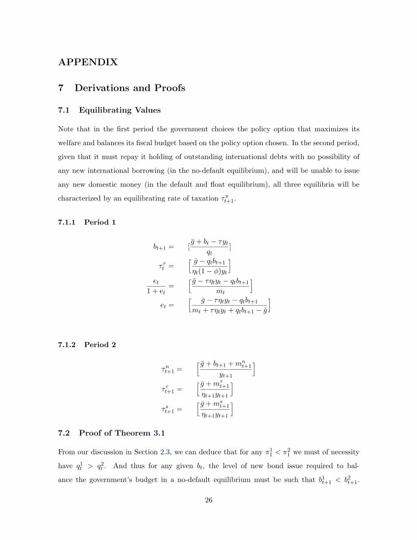
7.1 Equilibrating Values
Note that in the first period the government choices the policy option that maximizes its
welfare and balances its fiscal budget based on the policy option chosen. In the second period,
given that it must repay it holding of outstanding international debts with no possibility of
any new international borrowing (in the no-default equilibrium), and will be unable to issue
any new domestic money (in the default and float equilibrium), all three equilibria will be
characterized by an equilibrating rate of taxation τπt+1.
7.1.1 Period 1
bt+1 = [g + bt − τyt
qt]
τ τt =
[ g − qtbt+1
ηt(1− φ)yt
]et
1 + et=
[ g − τηtyt − qtbt+1
mt
]et =
[ g − τηtyt − qtbt+1
mt + τηtyt + qtbt+1 − g
]
7.1.2 Period 2
τnt+1 =
[ g + bt+1 + mnt+1
yt+1
]τ τt+1 =
[ g + mτt+1
ηt+1yt+1
]τ st+1 =
[ g + mst+1
ηt+1yt+1
]7.2 Proof of Theorem 3.1
From our discussion in Section 2.3, we can deduce that for any π11 < π2
1 we must of necessity
have q1t > q2
t . And thus for any given bt, the level of new bond issue required to bal-
ance the government’s budget in a no-default equilibrium must be such that b1t+1 < b2
t+1.
26
And consequently from Eq. 10 we must also have that cnt+1(π
11, π2) > cn
t+1(π21, π2) since
τnt+1(π
11, π2) < τn
t+1(π21, π2). Therefore,
V ng (π1
1, π2) = u(ct) + βEtu[cnt+1(π
11, π2)]
≥ u(ct) + βEtu[cnt+1(π
21, π2)]
= V ng (π2
1, π2)
7.3 Proof of Theorem 3.2
Consider two levels of outstanding debt stock that have become due in the first period,
given by b1t < b2
t . Ceteris paribus, this implies that the level of new bond issue required to
balance the government’s fiscal budget in a no-default equilibrium in the first period must
be such that b1t+1 < b2
t+1. Then from Eq. 10 we know that cnt+1(b
1t+1) > cn
t+1(b2t+1) since
τnt+1(b
1t+1) < τn
t+1(b2t+1). Hence must we have that V n
g (b1t+1) > V n
g (b2t+1) and consequently
π11 < π2
1.
27
References
Aguiar, M. and Gopinath, G. (2004). Defaultable debts, interets rates and the current account.
Forthcoming in the Journal of International Economics.
Aizenman, J., Gavin, M., and Housmann, R. (2000). Optimal tax and debt policy with
endogenously imperfect creditworthiness. Journal of International Trade and Economic
Development, 9(4):367–395.
Bulow, J. and Rogoff, K. (1989). A constant recontracting model of sovereign debt. Journal
of Political Economy, 97(1):155–178.
Cline, W. R. (2003). Restoring economic growth in Argentina. World Bank Policy Research
Working Paper 3158.
Cole, H. and Kehoe, T. (2000). Self-fulfilling debt crises. Review of Economic Studies, 67:91–
11.
Drazen, A. (1998). Towards a political-economic theory of domestic debts. In Calvo, G. and
King, M., editors, The Debt Burden and its Consequences for Monetary Policy, volume 118,
pages 159–176, London. The International Economic Association, MacMillan.
Drazen, A. and Masson, P. R. (1994). Credibility of policies versus credibility of policymakers.
The Quarterly Journal of Economics, 109(3):735–754.
Eaton, J. and Gersovitz, M. (1981). Debt with the potential repudiation: Theoretical and
empirical analysis. Review of Economic Studies, 48:289–309.
Feenstra, R. C. (1986). Functional equivalence between liquidity costs and and utility of
money. Journal of Monetary Economics, 17:271–291.
Greenwood, J. (1983). Expectations, the exchange rate, and the current account. Journal of
Monetary Economics, 12:543–569.
IMF (2003). Argentina: Request for Stand-By Arrangement and request for extension of
Repurchase Expectations. Technical Report No. 03/392, International Monetary Fund,
Washington, D.C.
28
Irwin, G. (2004). Currency boards and currency crises. Oxford Economics Papers, 56:64–87.
Jeanne, O. (1997). Are currency crises self-fulfilling? Journal of International Economics,
43:263–286.
Jeanne, O. and Masson, P. (2000). Currency crises, sunspots and markov-switching regimes.
Journal of International Economics, 50:327–350.
Komulaninen, T. (2004). Essays on Financial Crises in Emerging Markets. PhD thesis, Kurku
School of Economics and Business Administration, Helsinki.
Marshall, D. A. (1992). Inflation and asset returns in a monetary economy. The Journal of
Finance, 47(4):1315–1342.
Mulraine, M. L. B. (2004). An analysis of the 2002 Argentine currency crisis. University of
Toronto, Mimeo.
Obstfeld, M. (1995). Models of currency crises with self-fulfilling features. European Economic
Review, 40:1037–1047.
Rebelo, S. and Vegh, C. A. (2002). When is it optimal to abandon a fixed exchange rate.
Mimeo.
Walsh, C. E. (2003). Monetary Theory and Policy. The MIT Press, Cambridge, Massachusetts,
2nd edition.
Yue, V. Z. (2005). Sovereign default and debt renegotiation. New York University, Mimeo.
29
Table 1: Parameter Values Used:
Parameters: Definitions:
β = 0.962 Constant annual discount factor
r∗t = 0.040 Risk-free world interest rate
τ = 0.237 Constant tax rate
g = 0.250 Annual government expenditure
η = 0.92 One minus the endowment loss
σ = 2.000 Coefficient of Risk aversion
φ = 0.015 Tax policy adjustment loss
ε = 0.0014 Transaction cost parameter
30
Figure 1: First Period Consumption Level
00.2
0.40.6
0.81
0
0.2
0.4
0.6
0.8
10.78
0.79
0.8
0.81
0.82
0.83
0.84
0.85
0.86
Expected Probability of FloatExpected Probability of Default
First P
eriod C
onsum
ption
31
Figure 2: Actual probability of Default
00.2
0.40.6
0.81
0
0.2
0.4
0.6
0.8
1
0.4
0.5
0.6
0.7
0.8
0.9
1
Expected Probability of FloatExpected Probability of Default