A MONTE CARLO EVALUATION OF THE POWER OF SOME TESTS FOR HETEROSCEDASTICITY* ± W.E. Griffiths and K. Surekha No.19 - August 1985 ~’Surekha is with the Indian Statistical Institute in Calcutta. Typist: Val Boland ISSN 0157-0188 ISBN 0 85834 598 6
Transcript
A MONTE CARLO EVALUATION OF THE POWER OFSOME TESTS FOR HETEROSCEDASTICITY*
±W.E. Griffiths and K. Surekha
No.19 - August 1985
~’Surekha is with the Indian Statistical Institute in Calcutta.
Typist: Val Boland
ISSN 0157-0188
ISBN 0 85834 598 6
i. Introduction
It is well known that in the presence of heteroscedasticity of error
variances, the least squares method has two major drawbacks: (i) ineffi-
cient parameter estimates and (ii) biased variance estimates which make
standard hypothesis tests inappropriate. The importance of tests for
heteroscedasticity is well recognized and a large number of tests have
been proposed. There are test procedures for establishing a specific
form of heteroscedasticity, and a wide range of tests for detecting only
the presence or absence of heteroscedasticity. See, for example, Goldfeld
and Quandt (1965), Rutemiller and Bowers (1968), Glejser (1969) t Ramsey
(1969), Theil (1971), Harvey and Phillips (1974), Harvey (1976), Bickel
(1978), Szroeter (1978), Breusch and Pagan (1979), Harrison and McCabe
(1979), White (1980), Carroll and Rupert (1981), King (1982), Barone-Adesi
and Talwar (1983), Buse (1984), Ali and Giaccotto (1984), Evans and King
(1985), and Judge et al. (1985, Chapter ii). The various tests proposed
by these authors have been well reviewed in the last three listed
references, and so a further review will not be attempted here. We are
concerned with evaluating a computationally simple asymptotic test which
was proposed by Szroeter (1978) and which appears to have been overlooked
in the studies listed above. This test, originally designed for structural
and reduced form relations in dynamic simultaneous equation models can,
under appropriate assumptions, also be used to test for heteroscedasticity
in linear regression models. A finite sample version of the test was shown
by King (1982) to be approximately locally best invariant under quite
general conditions and its power has compared favourably with that of a
number of other test procedures [Evans and King (1985)]. However, because
the critical value of the finite sample version of the test depends on the
set of regressors, this test is computationally demanding and unlikely to
be computed routinely in standard econometric computer packages. In
contrast, routine calculation of the asymptotic test could easily take
place, in much the same way as the Durbin-Watson statistic is routinely
computed to test for autocorrelation. See Harrison (1980) for a discussion
on the relative computational ease of a large number of tests for
heteroscedasticity.
We have chosen to compare Szroeter’s asymptotic test with three
others - the Goldfeld-Quandt test [Goldfeld and Quandt (1965)], the
Breusch-Pagan test [Breusch and Pagan (1979)], and BAMSET [Ramsey (1969)].
The Goldfeld-Quandt (G-Q) test has been chosen because it appears to be
the most popular test in applied econometrics and its performance has been
found to be satisfactory in many of the earlier studies. The Lagrange
multiplier (LM) test proposed by Breusch and Pagan (B-P) is also popular
and is simple to compute. It, too, has been found to be quite powerful
in the presence of heteroscedasticity. The test BAMSET has been included
following a suggestion from a referee that its performance is likely to be
less sensitive to the assumption that, under the alternative hypothesis of
heteroscedasticity, the observations can be ordered according to increasing
variances.
Monte Carlo methods are used to examine the four test procedures for
two different heteroscedastic variance structures with varying degrees of
heteroscedasticity, and for small and large samples. Our results indicate
that when it is possible to order the observations according to increasing
variances, Szroeter’s test is more powerful than the remaining three.
When the observations have not been ordered the performances of Szroeter’s
test, BAMSET and the G-Q test all fall dramatically and, as hypothesized
by the referee, BAMSET is better than the other two. The B-P test does
not depend on whether or not the observations are ordered, but does depend
on similarly strong prior information. Details of the variance
specifications and the tests are given in section 2. The set-up of the
Monte Carlo experiment and the results are presented in sections 3 and
4, respectively.
Variance Structures and Tests for Heteroscedasticity
Consider a linear regression model
Yt = Xt8 + ut’ t=l,2, ..... T, (i)
where Xt = (l,xt) contains the constant term and the t-th observation on
an explanatory variable, Yt is the t-th observation on a dependent
variable, 8 is a (2 × i) vector of parameters, and the ut are unobservable
normal random errors with mean zero and variances as specified below. We
restrict 8 and Xt to be of dimension 2 because this is in line with the
design of our Monte Carlo experiment, not because it is necessary for
carrying out the tests. Two types of variance structures are considered.
The first specification is
V(ut) = ~2t = exp(Zt~) = kxXt, (2)
where Zt = (i, log xt), and 6 = (log k,x)’ This model has been
discussed by Geary (1966), Park (1966), Lancaster (1968), Kmenta (1971),
and Harvey (1976), and, following Harvey, we shall refer to it as the
multiplicative heteroscedastic model. The second variance assumption is
2 2 2 2V(ut) = ot = (Xta) = a0(I + Ixt)
(3)
where a = (a0,al)’, I = ~i/~0 and Xt = (l,xt). This model has been
studied by Rutemiller and Bowers (1968), Glejser (1969) and Harvey (1974)
and we will refer to it as the additive heteroscedastic model.
We shall now briefly describe the four tests°
Szroeter’s Test
To begin we assume that in model (i) the exact form of the variances
(o~) may not be known but that all the observations can be arranged in
2 2~ ot t=2 3,...,T. This can be done either withsuch a way that ot_1 , ,
reference to certain exogenous variables appearing in our model (xt in our
case), or on the basis of predictive values of Yt based on OLS estimates.^ ^
If et = Yt - XtS’ where 8 is any consistent estimator of 8, the test
statistic is defined by
Q = T(h - ~)/ (ht - ~) ½ (4)
where h = 7.twtht,2 2
wt = et/7~tet, ~ = T-iZtht, and ht is a set of T
nonstochastic scalars having the property that ht ~ hs if t > s.
2 2Under the null hypothesis H0: ot = °t-l’ t=2,3,...,T against the
2 2alternative hypothesis HI: ~t > ~t-l’ Q follows a limiting normal
distribution with mean zero and variance unity°
If we let ht = t, t=l,2,...,T, the test statistic can be written
as
(5)
where ~2 2
= Ettet/Ztet. The test statistic (5) is very simple to compute,
and, because it is asymptotic N(0,1), the test is easy to apply. The
observations for models (2) and (3) can be arranged according to
increasing variances by arranging the x’s in ascending order° Also, for
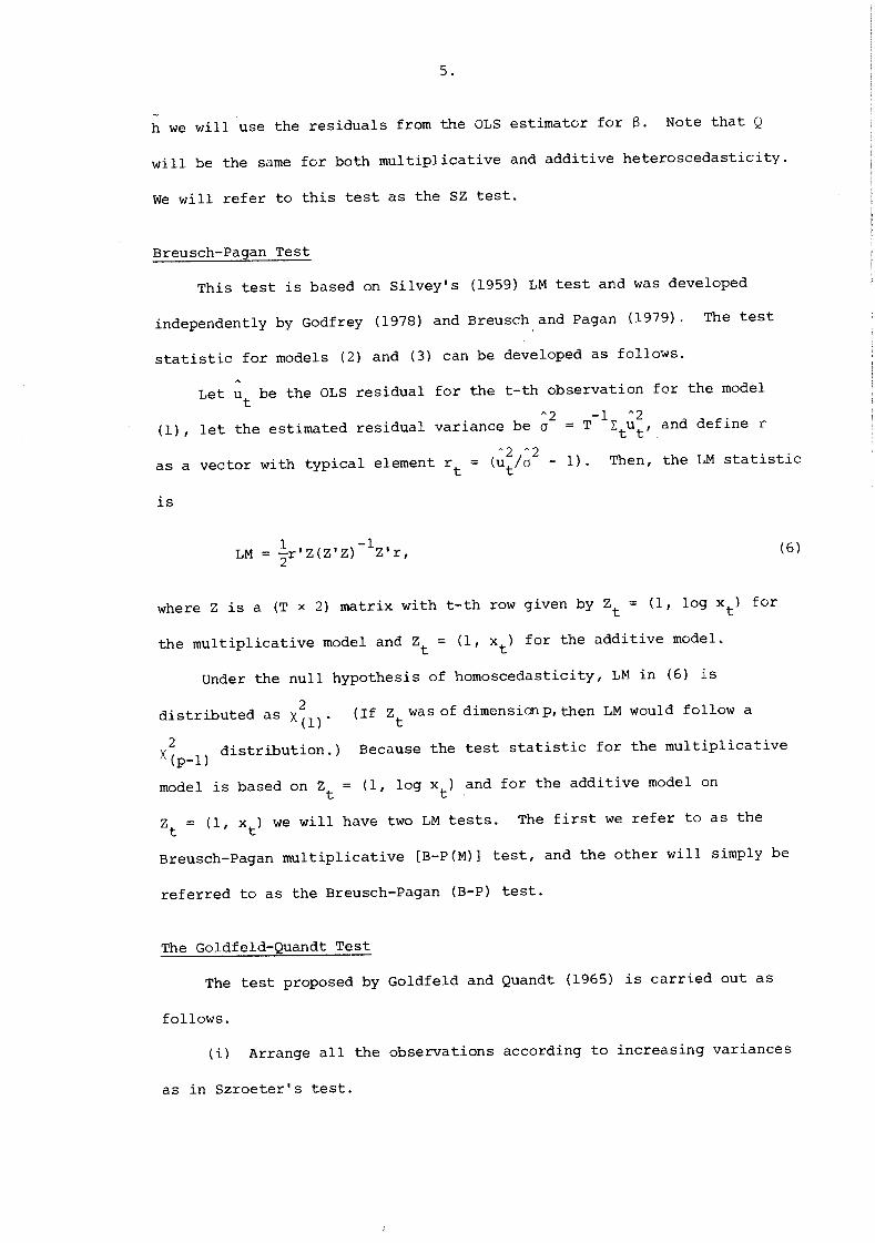
h we will use the residuals from the OLS estimator for 8. Note that Q
will be the same for both multiplicative and additive heteroscedasticity.
We will refer to this test as the SZ test.
Breusch-Pagan Test
This test is based on Silvey’s (1959) LM test and was developed
independently by Godfrey (1978) and Breusch and Pagan (1979). The test
statistic for models (2) and (3) can be developed as follows.^
Let ut be the OLS residual for the t-th observation for the model^2 -i ^2
(i), let the estimated residual variance be ~ = T Ztut, and define r
as a vector with typical element rt = (~/~2 i). Then, the LM statistic
is
LM ~r’Z(Z’Z)-Iz’= r, (6)
where Z is a (T × 2) matrix with t-th row given by Zt = (i, log xt) for
the multiplicative model and Zt = (I, xt) for the additive model~
Under the null hypothesis of homoscedasticity, LM in (6) is
2distributed as × (1) " (If Zt was of dimensicn p, then LM would follow a
2 distribution.) Because the test statistic for the multiplicative× (p-l)
model is based on Zt = (i, log xt) and for the additive model on
Zt = (i, xt) we will have two LM tests. The first we refer to as the
Breusch-Pagan multiplicative [B-P(M)] test, and the other will simply be
referred to as the Breusch-Pagan (B-P) test.
The Goldfeld-Quandt Test
The test proposed by Goldfeld and Quandt (1965) is carried out as
follows.
(i) Arrange all the observations according to increasing variances
as in Szroeter’s test.
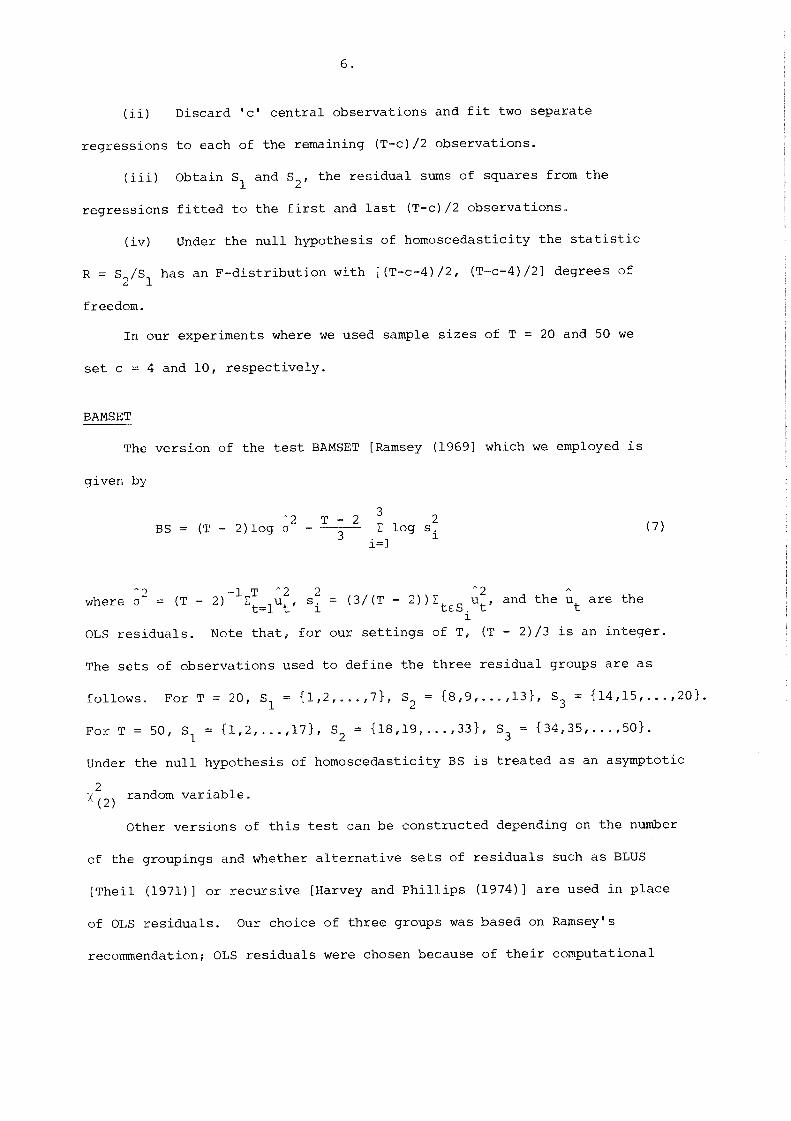
(ii) Discard ’c’ central observations and fit two separate
regressions to each of the remaining (T-c)/2 observations.
(iii) Obtain S1 and S2, the residua! sums of squares from the
regressions fitted to the first and last (T-c)/2 observations.
(iv) Under the null hypothesis of homoscedasticity the statistic
R = S2/S1 has an F-distribution with [(T-c-4)/2, (T-c-4)/2] degrees of
freedom.
In our experiments where we used sample sizes of T = 20 and 50 we
set c = 4 and I0, respectively.
BAMSET
The version of the test BAMSET [Ramsey (1969] which we employed is
given by
3^2 T- 2 2BS = (T - 2)log ~ 3 Z log s.
1i=l
(7)
^2 -i T ^2 2 ^2 and the ut are thewhere ~ = (T - 2) Et=lUt, s.l = (3/(T- 2))Zt~s.Ut,1
OLS residuals. Note that, for our settings of T, (T - 2)/3 is an integer.
The sets of observations used to define the three residual groups are as
follows. For T = 20, S1 = {1,2 .... ,7}, S2 = {8,9, .... 13}, S3 = {14,15 .... ,20}.
For T = 50, S1 = {1,2, .... 17}, S2 = {18,19, .... 33}, S3 = {34,35, .... 50}.
Under the null hypothesis of homoscedasticity BS is treated as an asymptotic
2 random variable.X(21
Other versions of this test can be constructed depending on the number
of the groupings and whether alternative sets of residuals such as BLUS
[Theil (1971)] or recursive [Harvey and Phillips (1974)] are used in place
of OLS residuals. Our choice of three groups was based on Ramsey’s
recommendation; OLS residuals were chosen because of their computational
ease and their apparent superiority in experiments conducted by Ramsey
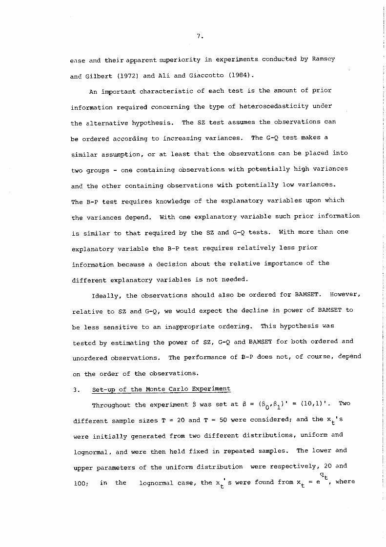
and Gilbert (1972) and Ali and Giaccotto (1984).
An important characteristic of each test is the amount of prior
information required concerning the type of heteroscedasticity under
the alternative hypothesis. The SZ test assumes the observations can
be ordered according to increasing variances. The G-Q test makes a
similar assumption, or at least that the observations can be placed into
two groups - one containing observations with potentially high variances
and the other containing observations with potentially low variances.
The B-P test requires knowledge of the explanatory variables upon which
the variances depend. With one explanatory variable such prior information
is similar to that required by the SZ and G-Q tests. With more than one
explanatory variable the B-P test requires relatively less prior
information because a decision about the relative importance of the
different explanatory variables is not needed.
Ideally, the observations should also be ordered for BAMSET. However,
relative to SZ and G-Q, we would expect the decline in power of BAMSET to
be less sensitive to an inappropriate ordering. This hypothesis was
tested by estimating the power of SZ, G-Q and BAMSET for both ordered and
unordered observations. The performance of B-P does not, of course, depend
on the order of the observations.
3. Set-up of the Monte Carlo Experiment
Throughout the experiment 8 was set at 8 = (80,81)’ = (i0,i)’ Two
different sample sizes T = 20 and T = 50 were considered; and the xt’s
were initially generated from two different distributions, uniform and
lognormal, and were then held fixed in repeated samples. The lower and
upper parameters of the uniform distribution were respectively, 20 and
qti00; in the lognormal case, the xt s were found from xt e , where
the qt s were generated from N(3.8, 0°42)° Five thousand replications
were generated for each combination of sample size, regressor type and
error variance model. The ut’s were drawn from a normal distribution
with mean zero and variances given by (2) and (3) for the m111tiplicative
and additive models, respectively° The severity of the heteroscedasticity
was controlled by varying the parameters ~ and l; we considered 18 values
of i between 0 and 2.0, 55 values of y between -7 and 7, and an additional
6 values of ~ equal to i0, 50, I00, 500, i000 and 5000~ For negative
values of ¥ the observations were ordered according to decreasing rather
than increasing values of xt. The powers of all five tests~ SZ,
B-P(M), G-Q, and BAMSET were estimated by calculating the proportion of
rejections in 5000 replications at a 5% level of significance°
4. Results
A convenient measure of the degree of heteroscedasticity which was
suggested by Surekha (1980), and later used by Evans and King (1985), is
the coefficient of variation of the variances (C of V). This measure is
invariant with respect to the units of measurement of the variables and,
for a given x-vector (lognormal or uniform), it turns out to be the major
determinant of the powers of the tests. In Table 1 we have presented the
estimated powers of the tests for some selected values of I and 7 which
lead to similar values of the C of Vo Whether or not the heteroscedasticity
is multiplicative or additive has little bearing on the power of each test
when the x-vector is the same and the C of V~s are similar° In fact, in
the last four rows of the Table the powers are identical for identical
C of V’so This result generally held throughout, although there were some
instances where there were very slight differences in the powers for
identical C of V’so
Another result illustrated by Table 1 is that, for a given C of V,
the power of each test is greater for uniform x than for lognormal x.
This result also held throughout, except for a few cases when the C of
V was less than 0.3.
Considering negative values of ~ for the multiplicative model is
equivalent to considering two more types of x for that model - one which
is the inverse of uniformally distributed x, and one which is the inverse
of lognormally distributed x. A general comparison of these results with
those for ¥ > 0 showed that the powers of the tests for y > 0 tended to
be greater than the powers of the corresponding tests for ~ < 0 and
similar C of V’s.
When I was increased from 50 to 5000 the C of V’s and the powers of
the tests did not change, suggesting that there is an upper bound to the
degree of heteroscedasticity (C of V) which can be modelled using the
additive specification. Investigating this matter further, we considered
the square of the C of V defined by
2
(C of V) 2 = Z°t (8)
2Substituting for o
tfrom (3) and taking limits yielded
= T-I 2 (9)( ~x2t)
Thus, there is indeed an upper bound to the degree of heteroscedasticity
which can be modelled with an additive heteroscedastic specification. A
similar exercise applied to the multiplicative specification yielded an
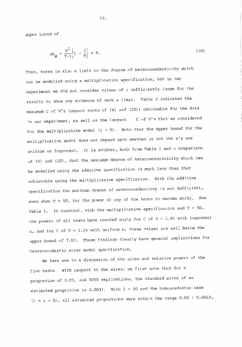
i0o
upper bound of
T2 (I0)
Thus, there is also a limit to the degree of heteroscedasticity which
can be modelled using a multiplicative specification, but in our
experiment we did not consider values of y sufficiently large for the
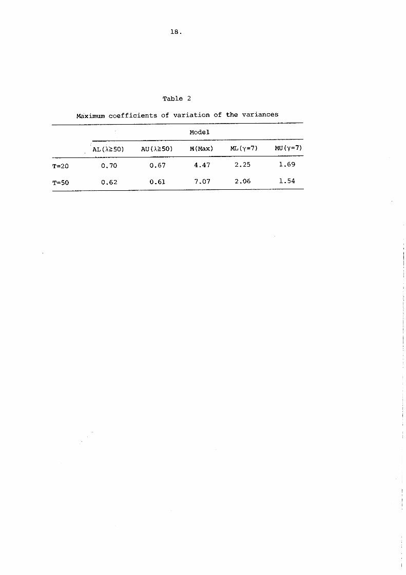
results to show any evidence of such a limit° Table 2 indicates the
maximum C of V’s (square roots of (9) and (i0)) obtainable for the data
in our experiment, as well as the largest C of V’s that we considered
for the multiplicative model (y > 0) o Note that the upper bound for the
multiplicative model does not depend upon whether or not the x’s are
uniform or lognormalo It is evident, both from Table 2 and a comparison
of (9) and (i0), that the maximum degree of heteroscedasticity which can
be modelled using the additive specification is much less than that
achievable using the multiplicative specification° With the additive
specification the maximum degree of heteroscedasticty is not sufficient~
even when T = 50, for the power of any of the tests to become unity. See
Table io In contrast, with the multiplicative specification and T = 50,
the powers of all tests have reached unity for C of V = 1.81 with lognormal
x, and for C of V = 1.24 with uniform x; these values are well below the
upper bound of 7°07° These findings clearly have general implications for
heteroscedastic error model specification.
We turn now to a discussion of the sizes and relative powers of the
five tests° With respect to the sizes~ we first note that for a
proportion of 0°05, and 5000 replications, the standard error of an
estimated proportion is 0o0031o With T = 50 and the homoscedastic case
(~ = y = 0), all estimated proportions were within the range 0.05 ± 0°0062,
ii.
although the B-P and B-P(M) tests, with sizes of 0.047 and 0.044 for
uniform x and 0.044 and 0.045 for lognormal x, were at the low end of
this range. In contrast, with T = 20 only the finite sample G-Q test
had an estimated size within the specified confidence interval. All
the asymptotic tests (SZ, B-P, B-P(M) and BAMSET) had finite sample
sizes well below the specified 5% significance level. These sizes
ranged from 0.031 for SZ and BP with lognormal x to 0.038 for BAMSET
with uniform x. Similar results for the B-P test were reported by
Godfrey (1978) and Breusch and Pagan (1979).
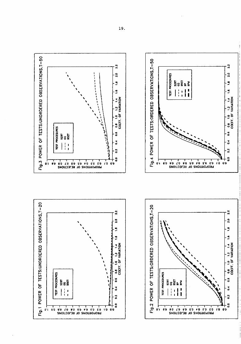
As mentioned earlier, the relative powers of the various tests are
likely to depend heavily on whether or not the observations have been
ordered according to increasing variances. In Figures 1 to 4 we have
graphed the powers for both ordered and unordered observations for the
multiplicative model with lognormal x and ¥ > 0. These powers are graphed
against the C of V since it is a reasonable measure of the degree of
heteroscedasticity, and the results for additive heteroscedasticity (and
lognormal x) are essentially identical, except that they do not extend
beyond C of V’s greater than 0.70 (T = 20) or 0.62 (T = 50). We have
not presented the results for ~ < 0 and uniform x because these cases led
to identical conclusions about the r~tiue power8 of the tests.
From Figures 2 and 4 we observe that, when the observations have
been ordered according to increasing variances, the SZ test is most
powerful, followed by the G-Q test, the B-P and B-P(M) tests (which are
very similar), and BAMSET. For T = 20 the G-Q test is better than SZ
for low and high C of V’s, although the difference in performance at the
low end seems to occur because SZ has incorrect finite sample size.
Figures 1 and 3 show the powers of the SZ, G-Q and BAMSET tests
when the observations have not been ordered according to increasing
variances. The powers are very similar, and very poor, for C of V’s
up to 0.6. After this point BAMSET is clearly best since its power
[unction begins to rise more steeply while the other power functions
only gradually increase (T = 50), or ~ (T = 20). With uniform x
(which we have not graphed), the performance of BAMSET was similar,
but the power functions of SZ and G-Q gradually increased for T : 20 and
fell for T = 50. These results, and an examination of the x-vectors,
showed that whether the powers of the SZ and G-Q tests increased or
remained below their size did not depend on sample size but rather on the
distribution of the unordered x’so
5. Conclusions
If it is impossible to order the observations according to increasing
variances, and there is insufficient prior information to relate the
variances to some explanatory variable(s), then from the tests that we
have considered, only BAMSET is viable. However, its power is extremely
poor when compared with that which can be achieved, by any of the tests,
if the observations are appropriately ordered° Such an ordering leads to
a clear prescription for Szroeter’s test. Given the ease with which both
Szroeter’s test and BAMSET can be computed, and given their respective
superior performances under circumstances of some and no prior information
about variances, we feel that serious consideration should be given to the
routine calculation of both these statistics.
The maximum degree of heteroscedasticity which can be modelled using
an additive heteroscedastic specification is much less than that which can
be achieved using a multiplicative heteroscedastic specification. Due
consideration should be given to this fact when choosing a variance model
and enthusiastic research assistance. An earlier version of this paper
was written while Griffiths was visiting the Department of Economics,
University of Illinois, Urbana-Champaign.
14.
References
Ali, M.M. and C. Giaccotto, 1984, A study of several new and existing
tests for heteroscedasticity in the general linear model, Journal
of Econometrics, 26, 355-374.
Barone-Adesi, G. and P.P. Talwar, 1983, Market models and hetero-
scedasticity of residual security returns, Journal of Business
and Economic Statistics, I, 163-168.
Bickel, P.J., 1978, Using residuals robustly I: Tests for hetero-
scedasticity, nonlinearity, Annals of Statistics, 6, 266-269.
Breusch, T.S. and A.R. Pagan, 1979, A simple test for heteroscedasticity
and random coefficient variation, Econometrica, 47, 1287-1294.
Buse, A., 1984, Tests for additive heteroskedasticity: Goldfeld and
Quant revisited, Empirical Economics, 9, 199-216.
Carroll, R.J. and D. Ruppert, 1981, On robust tests for heteroscedasticity,
Annals of Statistics, 9, 205-209.
Evans, M.A. and M.L. King, 1985, A point optimal test for heteroscedastic
disturbances, Journal of Econometrics, 27, 163-178.
Geary, R.G., 1966, A note on residual heterovariance and estimation
efficiency in regressions, American Statistician, 20, 30-31.
Glejser, H., 1969, A new test for heteroscedasticity, Journal of the
American Statistical Association, 64, 316-323.
Godfrey, L.G., 1978, Testing for multiplicative heteroscedasticity,
Journal of Econometrics, 8, 227-336.
Goldfeld, S.M. and R.E. Quandt, 1965, Some tests for homoscedasticity,
Journal of the American Statistical Association, 60, 539-547.
Goldfeld, S.M. and R.E. Quandt, 1972, Nonlinear methods in econometrics,
Amsterdam: North Holland.
Harrison, M.J. and B.P.M. McCabe, 1979, A test for heteroscedasticity
based on ordinary least squares residuals, Journal of the American
Statistical Association, 74, 494-500.
15.
Harvey, A.C., 1974, Estimation of parameters in a heteroscedastic
regression model, paper presented at the European Meeting of the
Econometric Society, Grenoble.
Harvey, A.C., 1976, Estimating regression models with multiplicative
heteroscedasticity, Econometrica, 44, 460-465.
Harvey, A.Co and G.D.A. Phillips, 1974, A comparison of the power of
some tests for heteroscedasticity in the general linear model,
Journal of Econometrics, 2, 307-316.
Judge, G.G., W.E. Griffiths, R.C. Hill, H. Lutkepohl and T.-C. Lee,
1985, The theory and practice of econometrics, New York, John
Wiley and Sons.
King, M.L., 1982, A bounds test for heteroscedasticity, working paper,
Department of Econometrics and Operations Research, Monash
University, Australia.
Kmenta, J., 1971, Elements of econometrics, New York, The Macmillan
Company.
Lancaster, T., 1968, Grouping estimators on heteroscedastic data,
Journal of the American Statistical Association, 63, 182-191.
Park, R.E., 1966, Estimation with heteroscedastic error terms,
Econometrics, 34, 888.
Ramsey, J.B., 1969, Tests for specification error in the general
linear model, Journal of the Roya! Statistical Society B, 31,
250-271.
Ramsey, J.B. and R. Gilbert, 1972, Some small sample properties of
tests for specification error, Journal of the American Statistical
Association, 67, 180-186.
Rutemiller, H.C. and D.A. Bowers, 1968, Estimation in a heteroscedastic
regression model, Journal of the American Statistical Association,
63, 552-557.
16.
$ilvey, S.D., 1959, The lagrangian multiplier test, Annals of Mathematical
Statistics, 30, 389-407.
Surekha, K., 1980, Contributions to Bayesian analysis in heteroscedastic
models, unpublished Ph.D. thesis, University of New England,
Armidale, Australia.
Szroeter, J., 1978, A class of parametric tests for heteroscedasticity
in linear econometric models, Econometrica, 46, 1311-1327.
Theil, H., 1971, Principles of econometrics, New York, Wiley.
White, H., 1980, A heteroskedasticity-consistent covariance matrix
estimator and a direct test for heteroskedasticity, Econometrica,
48, 817-838.
17.
Table 1
Powers of tests for selected models and parameter values
Tests
Modela Param C of V SZ GQ BP BPM
AL I=.04 .410 ¯534 .464 .416 .400
ML 7=1.35 .416 .557 .489 .429 .421
AO I=.03 .412 .597 .541 .470 .444
MU 7=1.25 .406 .591 .536 .461 .446
AL I=500 .619 .819 .764 .703 .718
ML 7=2 .619 .819 .764 ¯703 ¯718
AU I=500 .608 .887 .847 .800 .812
MU 7=2 .608 .887 .847 .800 .812
BMSET
.275¯ 294.345.343
.568
.568
.692.692
aThe code for model type is M: multiplicative, A: additive,U: uniform and L: lognormal
18.
Table 2
Maximum coefficients of variation of the variances
Model
AL (I>50) AU (I_>_50) M (Max) ML (%,=7) MU (y=7)
T=20 0o 70 0.67 4.47 2.25 1.69
T=50 0.62 0.61 7.07 2.06 i. 54
o
I I I I I ! I I0"1 ~’0 g’O L’O g’O g’O t’O E’O ~’0 1,’0 0"0
SNOI.I.3]I’3EIJOSNOI.I.EIOdOBd
o
I I I I
0
WORKING PAPERS IN ECONOMETRICS AND APPLIED STATISTICS
The Prior Likelihood and Best Linear Unbiased Prediction in StochasticCoefficient Linear Models. Lung-Fei Lee and William E. Griffiths,No. 1 - March 1979.
Stability Conditions in the Use of Fixed Requirement Approach to ManpowerPlanning Models. Howard E. Doran and Rozany R. Deen, No. 2 - March1979.
A Note on a Bayesian Estimator in an Autocorrelated Error Model.William Griffiths and Dan Dao, No. 3 - April 1979.
On R2-Statistics for the General Linear Model with Nonscalar CovarianceMatrix. G.E. Battese and W.E. Griffiths, No. 4 - April 1979.
Constraction of Cost-Of-Living Index Numbers - A Unified Approach.D.S. Prasada Rao, No. 5 - April 1979.
~nission of the Weighted First Observation in an Autocorrelated RegressionModel: A Discussion of Loss of Efficiency. Howard E. Doran, No. 6 -June 1979.
Estimation of Household Expenditure Functions: An Application of a Classof Heteroscedastic Regression Models. George E. Battese andBruce P. Bonyhady, No. 7 - September 1979.
The Demand for Sawn Timber: An Application of the Diewert Cost Function.Howard E. Doran and David F. Williams, No. 8 - September 1979.
A New System of Log-Change Index Numbers for Multilateral Comparisons,D.S. Prasada Rao, No. 9 - October 1980.
A Comparison of Purchasing Power Parity Between the Pound Sterling andthe Australian Dollar - 1979. W.F. Shepherd and D.S. Prasada Rao,No. i0 - October 1980.
Using Time-Series and Cross-Section Data to Estimate a Production Functionwith Positive and Negative Marginal Risks. W.E. Griffiths andJ.R. Anderson, No. Ii - December 1980.
A Lack-Of-Fit Test in the Presence of Heteroscedasticity. Howard E. Doranand Jan Kmenta, No. 12 - April 1981.
On the Relative Efficiency of Estimators Which Include the InitialObservations in the Estimation of Seemingly Unrelated Regressionswith First Order Autoregres~ive Disturbances. H.E. Doran andW.E. Griffiths, No. 13 - June 1981.
An Analysis of the Linkages Between the Consumer Price Index and theAuerage Minimum Weekly Wage Rate. Pauline Beesley, No. 14 - July 1981.
An Error Components Model for Prediction of County Crop Areas Using Surveyand Satellite Data. George E. Battese and Wayne A. Fuller, No. 15 -February 1982.
2o
Networking or Transhipment? Optimisation Alternatives for Plant LocationDecisions. H.I. Toft and P.A. Cassidy, No. 16 - February 1985.
l)~agnostic Tests for the Partial Adjustment and Adaptive ExpectationsModels. H.E. Doran, No. 17 - Februa~l 1985.
A Further Consideration of Causal Relationships Between Wages and Prices.
J.W.B. Guise and P.A.A. Beesley, No. 18 - February 1985.