i
A New Approach to CNC Programming of Plunge
Milling
Sherif Mahmoud Mohamed Abdelkhalek
A Thesis
In The Department
of
Mechanical and Industrial Engineering
Presented in Partial Fulfillment of the Requirements
For the Degree of Doctor of Philosophy “Mechanical Engineering” at
Concordia University
Montreal, Quebec, Canada
September, 2013
© Sherif Abdelkhalek, 2013
ii
CONCORDIA UNIVERSITY
School of Graduate Studies
This is to certify that the thesis prepared
By: Sherif Mahmoud Mohamed Abdelkhalek .
Entitled: A New Approach to CNC Programming of Plunge milling .
and submitted in partial fulfillment of the requirements for the degree of
Doctor of Philosophy (Mechanical Engineering)
complies with the regulations of the University and meets the accepted standards with
respect to originality and quality.
Signed by the final examining committee:
Dr. Olga Ormandjieva . Chair
Dr. Hsi-Yung (Steve) Feng External Examiner
Dr. Wei-Ping Zhu External to Program
Dr. Ali Akgunduz Examiner
Dr. Sivakumar Narayanswamy Examiner
Dr. Zezhong C. Chen Thesis Supervisor
Approved by:
________________________________
Chair of Department or Graduate Program Director
__________________ ________________________________
Dean of Faculty
iii
ABSTRACT
A New Approach to CNC Programming of Plunge Milling
Sherif Abdelkhalek, PhD.
Concordia University, 2013.
In current industrial applications many engineering parts are made of hard materials
including dies, mold cavities and aerospace parts. Manufacturing these types of parts is
classified as pocket milling. By using the regular machining methods, pocket milling takes
a long time accompanied by high cost. Plunge milling, is a new machining strategy that
has proven to have an excellent performance in the rough machining of hard materials. In
plunge milling, the cutter is fed in the direction of the spindle axis, with the highest
structural rigidity which showed a very interesting performance in removing the excess
material rapidly in the rough operations. Mainly, according to the previous researchers,
two directions are adopted to improve the efficiency of the plunge milling process. First,
to reduce the cutting forces and increase chatter stability which attracts the majority of the
researchers. Second, to optimize the tool path planning which has less attention.
Therefore, in the first part of the research, a new practical approach is established in
optimized procedures to generate the tool paths for plunge milling of pockets, even for
these with free-form boundaries and islands. This innovative approach is proposed as
follows: (1) fill a pocket with minimum number of specified radii circles which are tangent
to each other and/or the pocket boundary without overlapping by building an algorithm
using the maximum hole degree (MHD) theory for solving the circle packing problem. (2)
cover the areas left between the non-overlapped circles by the same used specified radii.
Finally, solve the travelling sales man problem (TSP) for the circles with the same radii by
iv
using the simulated annealing algorithm. According to the results, this approach
significantly advances the tool path planning technique for pockets plunge milling.
In the second part of the research, a new algorithm is proposed to calculate the global
solution for constraint polynomial functions by using subtractive clustering which makes
the results more accurate and faster to be obtained. This part is extremely useful to calculate
the depth of cut for each plunging place in case of having a polynomial surface as a bottom
of the machined pocket with high accuracy, and less calculation time to avoid gauging
between the tool and the bottom surface.
The polynomial function can be classified according to the number of variables. In
the proposed research, the functions with one and two variables have more importance
because they graphically represent curves and surfaces which are the cases under study.
Since the polynomial function under study can be represented graphically according to the
number of the variables, the change in the function’s shape can be detected by the feature
recognition. The feature recognition is done for the function’s shape by calculating the
surface or curve curvature at the data points. The main procedure is; (1) identifying the
entire features of the objective function which are classified according to the curvature as
convex, concave, plane, and hyperbolic, (2) applying the sub-clustering technique for
convex and concave regions to find the approximated centers of these regions, and
eventually, (3) the clusters’ centers are calculated and used as initial points for local
optimization technique which gives the local critical point for each region. The local
minima are calculated, the global minimum is the minimum of the local minima.
v
DEDICATION
To my parents, my wife and my two kids; Roaa and Eyad.
vi
ACKNOWLEDGMENTS I would like to express my sincere thankfulness and appreciation to my supervisor
Dr. Chevy Chen for his guidance and support during the period of my PhD. work. His way
of guidance developed my research experience and significantly improved my research and
technical skills.
I greatly thank my parents and my wife for their support and patience. I also would
like to show my sincere appreciation to my former and present fellows in the CAD/CAM
laboratory (Maqsood Ahmed Khan, Shuangxui Xie, Mahmoud Rababah, Muhammad
Wasif, Aqeel Ahmad, Liming Wang, Du Chun, Mohsen Habibi, Zaher Khattab, Yuansheng
Zhou, Ka Ho Yu, and Ruibiao Song). The friendly environment in the laboratory they have
created, in addition to the support I got from them, has encouraged me to pursue and
improve my ideas for the research.
vii
Table of contents
FIGURES ........................................................................................................................... X
TABLES ........................................................................................................................ XIV
CHAPTER 1 ....................................................................................................................... 1
1.1 INTRODUCTION ........................................................................................................... 1
1.1.1 Plunge milling .................................................................................................... 2
1.1.2 Pocket milling ..................................................................................................... 4
1.1.3 Ploynomial functions global optimization .......................................................... 4
1.2 PROBLEM STATEMENT ................................................................................................ 5
1.3 RESEARCH OBJECTIVES ............................................................................................... 7
1.4 DISSERTATION ORGANIZATION ................................................................................... 8
CHAPTER 2 ..................................................................................................................... 10
LITERATURE REVIEW ................................................................................................. 10
2.1 PLUNGE MILLING ...................................................................................................... 10
2.2 CIRCLE PACKING ...................................................................................................... 16
2.3 GLOBAL OPTIMIZATION OF POLYNOMIAL FUNCTIONS ............................................... 21
2.4 CLUSTERING TECHNIQUES ........................................................................................ 22
CHAPTER 3 ..................................................................................................................... 24
POLYNOMIAL FUNCTION GLOBAL OPTIMIZATION BY USING SUBTRACTIVE
CLUSTERING TECHNIQUE .......................................................................................... 24
3.1 INTRODUCTION ......................................................................................................... 24
viii
3.2 GEOMETRIC CHARACTERIZATION OF OBJECTIVE FUNCTIONS .................................... 26
3.2.1 One variable objective function ........................................................................ 26
3.2.2 Dual variables objective function ..................................................................... 28
3.3 CLUSTERING TECHNIQUE .......................................................................................... 33
3.3.1 Subtractive clustering method .......................................................................... 34
3.4 OPTIMIZATION TECHNIQUE ....................................................................................... 37
3.4.1 Patching ............................................................................................................ 37
3.4.3 Local optimization ............................................................................................ 38
3.5 APPLICATIONS .......................................................................................................... 39
3.5.1 One variable objective function case studies .................................................... 39
3.5.2 Two variables objective function case studies ................................................. 51
3.5.3 Comparison between our approach and PSO ................................................... 64
3.6 CONCLUSION ............................................................................................................ 64
CHAPTER 4 ..................................................................................................................... 66
PLUNGE MILLING TOOL PATH OPTIMIZATION .................................................... 66
4.1 INTRODUCTION ......................................................................................................... 66
4.2 CIRCLE PACKING MATHEMATICAL MODEL ................................................................ 67
4.2.1 Maximum hole degree theory ........................................................................... 67
4.2.2 Algorithm to fill a pocket with tangent circles of specified radii ..................... 68
4.2.3 Algorithm to cover the gaps between the non-overlapped with the minimum
number of specified radii circles ............................................................................... 89
4.3 TOOL PATH OPTIMIZATION ........................................................................................ 99
ix
4.3.1 Solving travelling salesman problem (TSP) by using simulated annealing
algorithm (SA) ......................................................................................................... 100
4.3.2 Pocket with island ........................................................................................... 104
4.3.3 Free form boundary pocket with island .......................................................... 107
4.3.4 Comparison between CP method and the current methods ............................ 110
4.3.5 Conclusion ...................................................................................................... 113
4.4 POCKET WITH SCULPTURE BOTTOM SURFACE WITH POLYNOMIAL FUNCTION CASE
STUDY .......................................................................................................................... 114
4.4.1 Conclusion ...................................................................................................... 126
CHAPTER 5 ................................................................................................................... 127
CONCLUSION AND FUTURE WORK ....................................................................... 127
REFERANCES ............................................................................................................... 129
x
FIGURES
Figure (1. 1). Plunge milling. ...............................................................................................2
Figure (1. 2). Plunge milling processes. ..............................................................................3
Figure (1. 3). Generalized pocket illustration. .....................................................................4
Figure (2. 1). Comparison between conventional and plunge milling [5]. ........................12
Figure (2. 2). Comparison of cutting forces between plunge milling and side milling under
the condition of the same material cutting efficiency [6]. ...........................13
Figure (2. 3). Generation of Ocfill grid [7]. .......................................................................14
Figure (2. 4). Comparison of two methods (a) new method (b) Ocfill [8]. .......................15
Figure (2. 5). The step distance according to different serfaces’ shapes [9]. ....................16
Figure (2. 6). Circle Packing Hierarchy. ............................................................................17
Figure (2. 7). Unequal circle packing for circular and rectangular containers using MHD
method [12, 13]. ..........................................................................................18
Figure (2. 8). The corner occupying action (COA) for single circle [14]. .........................19
Figure (2. 9). Feasible distinct corner position of C5 [16]. ................................................20
Figure (2. 10). Feasible distinct corner positions of C3 in the strip [17]. ..........................21
Figure (3. 1). Curve patching. ............................................................................................27
Figure (3. 2). Surface patching. .........................................................................................28
Figure (3. 3). Pythagorean theory. .....................................................................................30
Figure (3. 4) Modified Pythagorean theory. ......................................................................31
Figure (3. 5). Surface shapes according to Gaussian and mean curvature. .......................32
xi
Figure (3. 6). Curve first case study. ..................................................................................41
Figure (3. 7). Curve second case study. .............................................................................44
Figure (3. 8). Curve third case study. .................................................................................47
Figure (3. 9). Curve fourth case study. ..............................................................................50
Figure (3. 10). Surface first case study. .............................................................................53
Figure (3. 11). Surface second case study. .........................................................................56
Figure (3. 12). Surface third case study. ............................................................................59
Figure (3. 13). Surface fourth case study. ..........................................................................62
Figure (4. 1). First algorithm flow chart ............................................................................69
Figure (4. 2). Convexity check. .........................................................................................70
Figure (4. 3). Boundaries gauge check. .............................................................................71
Figure (4. 4). General case. ................................................................................................73
Figure (4. 5). Circles overlapping check. ...........................................................................74
Figure (4. 6). Corner placements for a circle tangent to a boundary. ................................75
Figure (4. 7). Corner placements with other circles. ..........................................................80
Figure (4. 8). Check point inside a polygon. ......................................................................84
Figure (4. 9). Circles overlap check. ..................................................................................85
Figure (4. 10). Hole degree of a corner placement. ...........................................................87
Figure (4. 11). First case study for convex polygon. .........................................................88
Figure (4. 12). Second case study for polygon with some concave corners. .....................89
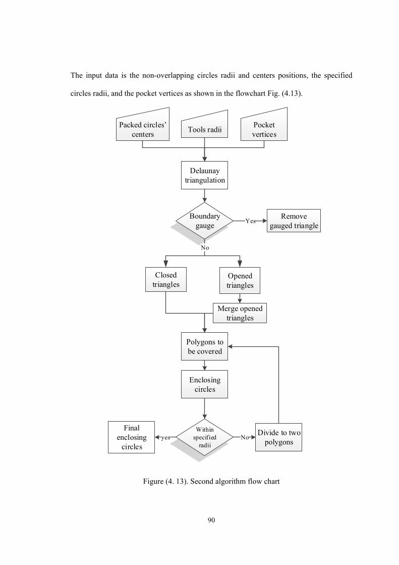
Figure (4. 13). Second algorithm flow chart ......................................................................90
Figure (4. 14). Convex hull boundary for Delaunay triangulation. ...................................91
xii
Figure (4. 15). Delaunay triangle. ......................................................................................92
Figure (4. 16). Edge flip to find max min angle. ...............................................................92
Figure (4. 17). Difference between triangles. ....................................................................93
Figure (4. 18). Merging the open triangles with the shared open edge. ............................94
Figure (4. 19). Smaller polygon connect the tangent points. .............................................95
Figure (4. 20). Circle enclosing the polygon. ....................................................................96
Figure (4. 21). First case study...........................................................................................98
Figure (4. 22). Second case study. .....................................................................................99
Figure (4. 23). Simulated annealing algorithm flow chart. ..............................................102
Figure (4. 24). Appling simulated annealing to optimize the tool path case study I. ......103
Figure (4. 25). Appling simulated annealing to optimize the tool path case study II. .....103
Figure (4. 26). Third case study for convex polygon with island. ...................................105
Figure (4. 27). Fourth case study for concave polygon with island. ................................106
Figure (4. 28). Case study V, the pocket and island boundaries are free form curve. .....108
Figure (4. 29). Appling the CP algorithm on case study V..............................................110
Figure (4. 30). Appling the OCfill method on case study V. ...........................................111
Figure (4. 31). Appling the Plunge milling feature in CATIA on case study V. .............112
Figure (4. 32). Applying the CP algorithm on the free form boundary case study. ........116
Figure (4. 33). Case study for pocket with sculpture bottom...........................................117
Figure (4. 34). Data points groups (Convex group “ . ”, Concave group “ * ”, hyperbolic
group “ o ”, and plane group “ x ”). ..........................................................118
Figure (4. 35). Concave data points clusters “*” with the clusters centers “□” and the
exact local maximum point “O” ................................................................119
xiii
Figure (4. 36). The cover circles and all the local maximum points “o”. ........................120
Figure (4. 37). The projected boundary of the circle on the bottom surface. ..................121
Figure (4. 38). Data points groups (Convex group “ □ ”, Concave group “o”), and Cluster
center “*”. ..................................................................................................123
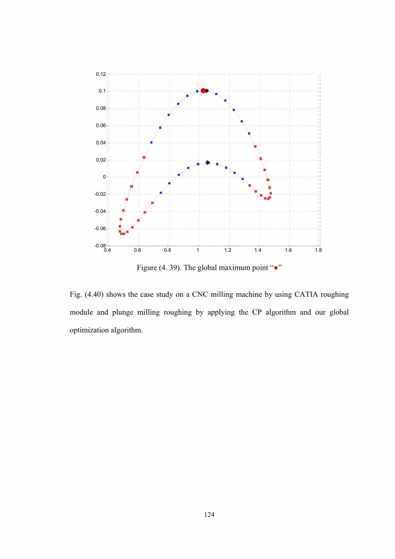
Figure (4. 39). The global maximum point “●” ...............................................................124
Figure (4. 40). Case study of pocket with free form boundary and sculpture bottom. ....125
xiv
TABLES
Table (3. 1). The Relation between the geometry shape and curve geometry features. ....27
Table (3. 2). The Relation among the geometry shape and surface geometry features. ....32
Table (3. 3). Case study I clusters centers. ........................................................................41
Table (3. 4). Case study I exact local minima. ...................................................................42
Table (3. 5). Case study II clusters centers. .......................................................................44
Table (3. 6) Case study II exact local minima. ..................................................................45
Table (3. 7). Case study III clusters centers. ......................................................................47
Table (3. 8). Case study III exact local minima. ................................................................47
Table (3. 9). Case study IV clusters centers. ......................................................................50
Table (3. 10). Case study IV exact local minima. ..............................................................51
Table (3. 11). Case study I clusters centers. ......................................................................53
Table (3. 12). Case study I exact local minima. .................................................................54
Table (3. 13). Case study II clusters centers. .....................................................................56
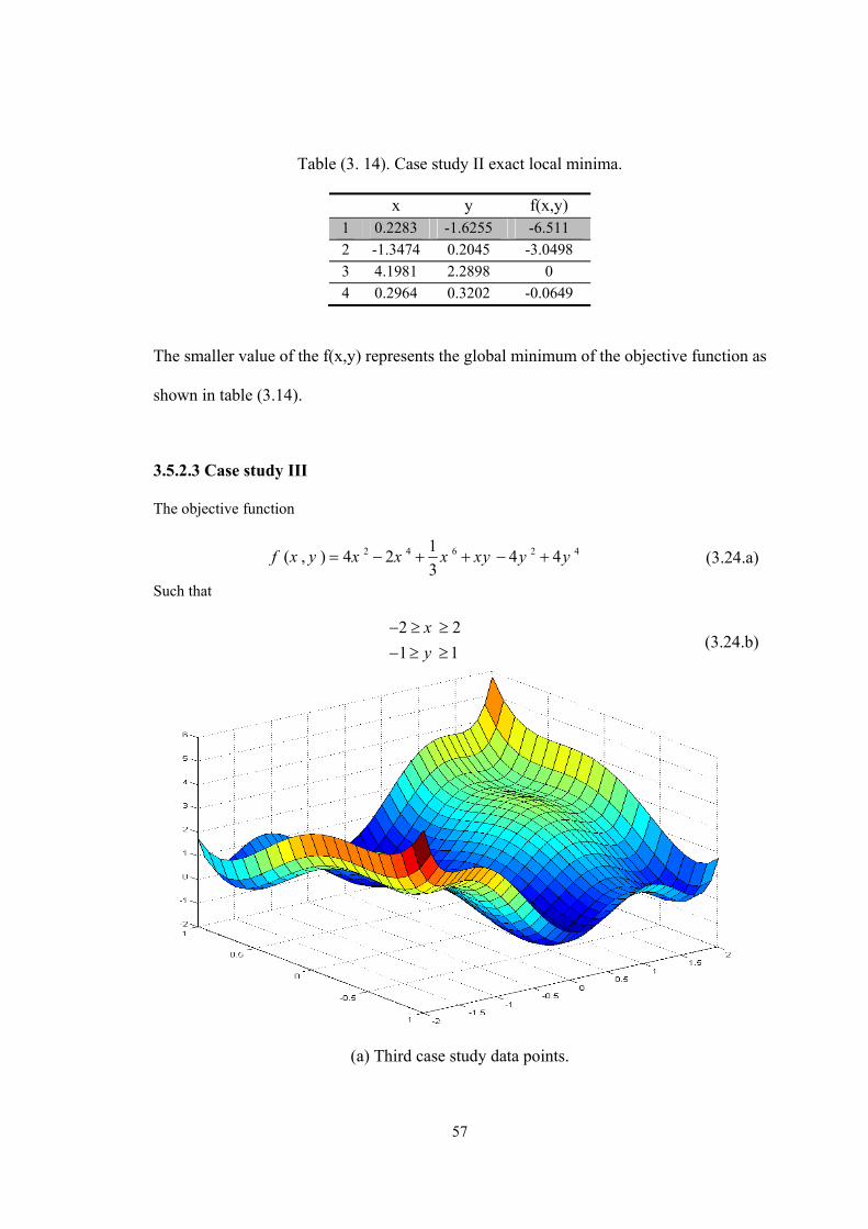
Table (3. 14). Case study II exact local minima. ...............................................................57
Table (3. 15). Case study III clusters centers. ....................................................................59
Table (3. 16). Case study III exact local minima. ..............................................................60
Table (3. 17). Case study III clusters centers. ....................................................................63
Table (3. 18). Case study III exact local minima. ..............................................................63
Table (3. 19). Comparison between our approach and PSO ..............................................64
Table (4. 1). First case study results. .................................................................................88
Table (4. 2). Second case study results. .............................................................................89
xv
Table (4. 3). First case study results. .................................................................................98
Table (4. 4). Second case study results. .............................................................................99
Table (4. 5). Case study III results. ..................................................................................105
Table (4. 6). Case study IV results. ..................................................................................107
Table (4. 7). Comparison between CP algorithm, OCfill method, and CATIA ..............113
Table (4. 8). Comparison between CP algorithm, OCfill method, and CATIA ..............116
Table (4. 9). Case study clusters centers. .........................................................................119
Table (4. 10). Case study exact local maxima. ................................................................120
1
Chapter 1
1.1 Introduction
CNC machining is considered as the core of manufacturing technology. The
machining operation is generally divided into two main processes which are distinguished
by the purpose and the cutting conditions; (1) roughing cuts, and (2) finishing cuts.
Roughing cuts are used to remove large amounts of material from the starting work piece
as rapidly as possible. This is done in order to produce a shape close to the desired form
while leaving some extra material on the work piece for a subsequent finishing operation.
Finishing cuts are used to complete the part and achieve the final dimension, tolerances,
and surface finish. Roughing cuts are done at high feeds and cutting depths with low cutting
speeds while finishing cuts are carried out at low feeds and cutting depths with high cutting
speeds.
For several decades, researchers dedicated great attention to improve the finishing
cuts seeking an increase in the machining efficiency while maintaining high machining
quality. According to many studies and researches, roughing cuts, (rough machining) could
take more than 60% of the total machining time, which attracted much academic and
industrial attention. To increase the efficiency of rough machining, especially for hard
materials, the emerging cutting strategy (plunge milling) was proposed as an effective
solution. Pockets are great examples for the parts with the higher amount of material to be
removed in the roughing step, which are widely used in the industry recently.
Optimization is the main tool to the improvement. Therefore the optimization will
have an important role in our research. The optimization is used to decrease the total
2
machining time, also our own optimization technique will be used to improve the efficiency
of the plunge milling process by calculating the accurate depth of cut.
1.1.1 Plunge milling
The plunge milling method is also known as the z-axis milling. In the plunge
milling process, the feed movement of the cutter is along the axial direction and provides
a combination between drilling and milling by using the bottom edge of the cutter [1], as
shown in Fig. (1.1); where ae is the radial cutting depth, and S is each step’s distance along
the side direction.
Figure (1. 1). Plunge milling.
There are three main types of the plunge milling process with different types of
plungers depending on the process configuration; (1) hole making, (2) hole enlarging, and
(3) intermittent plunge milling, as shown in Fig. (1.2)
3
(a) Hole making, (b) hole enlarging, and (c) intermittent.
Figure (1. 2). Plunge milling processes.
Compared to side milling, plunge milling has the following advantages: (1) high axial
rigidity for super alloy processing, (2) low requirement for radial force, reducing possibility
for work piece distortion, and producing better surface smoothness, (3) protecting cutters
from breaking, and (4) relatively stable, and small cutting force and vibrations. Because of
the mentioned advantages, plunge milling is perfectly suitable for roughing the high metal
removal rate parts like die mold cavities and, and parts related to aerospace industries. With
the lower radial cutting forces, this process is perfect for thin wall roughing. Dies, molds
cavities, thin wall parts … etc. are considered as pockets. Compared with side milling [2]
the axial cutting force of plunge milling is larger, but the radial cutting force is smaller.
Namely, the bearing capacity of the axial force is superior to the radial force of the cutter.
This makes use of the anisotropic characteristics of the force bearded by the cutter. As for
conditions of the large allowance removal for the materials that are difficult to cut as well
as the large length of the cutter, a larger cutting feed parameter can be given in plunge
milling which is suitable for machining pockets.
4
1.1.2 Pocket milling
Pocket milling is one of the most common operations in machining metal parts.
Pocket milling is defined as removing all the material inside some arbitrary closed
boundary of a work piece to a certain depth. Such a shape is frequently called a generalized
pocket, as shown in Fig. (1.3). Pockets are classified among the parts which have the
property of a large amount of the material has to be removed during the machining process.
Dies, molds cavities, and thin wall parts can be considered as pockets with a sculptured
bottom surface. As I will illustrate later in the literature review, the Plunge milling is
noticed to be better for pocket roughing in comparison to side milling.
Figure (1. 3). Generalized pocket illustration.
1.1.3 Ploynomial functions global optimization
By definition, polynomial is an expression consisting of a finite length which is
composed of variables and constants. The polynomial function may contain one or more
variables. It can also be of a single degree which is specified as linear, or more (quadratic,
cubic… nth) degree. The remarkable ability of the polynomial functions in modeling, attract
the attention of the optimization researchers. The industry is one of the important fields
5
which is affected by the polynomial functions’ ability in modeling, specially modeling the
surfaces and curves.
Because of the nature of the polynomial functions the global optimization is
considered as one of the interesting challenges. Calculating the global optimal solution for
a polynomial function is one of the great challenges in the optimization field. There are
many methods for calculating the global optimum like the deterministic methods (Branch
and bound, Cutting plane), the stochastic methods (Simulated annealing), the heuristics,
and metaheuristics methods (Genetic algorithm, practical swarm optimization, and ant
colony optimization). All of these methods have advantages and disadvantages; the main
disadvantages are the long computational time, and the low accuracy of the results. So our
objective is to establish a new approach to increase the accuracy and reduce the
computational time.
1.2 Problem statement
The pocket machining operations aim to remove all the material inside a pre-
defined boundary between two surfaces using minimal machining time. The only constraint
specified by the part geometry is the boundary of the pocket. As all of the machining
operations, the pocket machining is divided mainly into two steps, the rough machining
step and the finish machining step. The rough machining of a pocket may take more than
60% of the machining time which is a considerable amount. In addition, if the part material
is very hard or the pocket has a high depth, the roughing time will increase to more than
60% of the time. From the review, most of the authors adopted the plunge milling as the
6
most suitable process for the rough pocket machining because it has a high metal removal
rate.
The other problem we will discuss in our research is to find the global optimization
of the polynomial functions in accurate manner with less computational time. Our focus
will be on the polynomial functions with one and two variables. These types of polynomial
functions have many utilities in the industrial field since they can represent curves, and
surfaces. Finding the accurate global optimum solution of the polynomial function will be
very beneficial to improve the pocket plunge milling process.
In the approach, optimization of the tool path planning for the pocket plunge milling
is adopted. Taking into consideration, more than one plunger with different standard sizes
will be used, and different types of pocket boundary shapes will be applied. This work will
be for pockets with polygon boundary, pockets with polygon boundary with island, and
pockets with Free-form boundary.
Moreover, by solving the global optimization problem of the polynomial functions,
the pockets with sculptured bottom surface represented by polynomial functions will be
considered by calculating the proper depth of cut at each plunging place. This problem can
be formulated as covering a 2D pocket area by specified overlapped circles, and calculating
the accurate depth of cut for each plunging place to avoid gauging the bottom surface.
The problems can be listed as:
1. Using different sizes of standard plungers.
2. Filling the pocket area with the standard plungers in a decreasing order.
3. Plunging the pockets with Free-form boundary and island.
7
4. Calculating the accurate depth of cut at each plunging place to avoid gauging with
sculptured bottom surface.
1.3 Research objectives
The main objective of this research is to establish two new approaches. The first
approach is to generate the tool paths for plunge milling of pockets with free-form
boundaries and islands, and the second approach is a global optimization technique to find
the global solution of the polynomial functions with one, and two variables. The pockets
with sculptured bottom surfaces represented by polynomial functions will be considered
by integrating the two approaches. This research covers algorithms development, related
theorems establishment, computer program implement, and empirical verification. The
main features of the innovative integrated approach are (1) gouge-free plunging of pockets
with free-form boundaries, islands and sculptured bottom surface, and (2) optimized tool
paths for standard plungers that are available. This approach includes the following five
algorithms:
1. Fill a pocket with minimum number of specified radii circles which are tangent to
each other and/or the pocket boundary without causing any overlap by building an
algorithm using the maximum hole degree (MHD) theory for solving the circle
packing problem.
2. Cover the areas left between the non-overlapped circles by the same used specified
radii through building an algorithm to solve the minimal enclosing circle problem.
3. Solve the travelling sales man problem (TSP) for the centers of the circles with the
same radii.
8
4. Obtain the optimum tool path planning for the plunge milling of pockets with island
and free-form boundary.
5. Optimize the depth of cut for each plunging place in case of sculptured bottom
surface with polynomial function.
As a result, the final algorithm will be able to find the optimum plunging tool path for
pockets with free form boundaries and islands as well as the ability of using any number
of preselected tools with standard or modified diameters due to the re-sharpening process.
In addition, it has the ability to calculate the accurate depth of cut at each plunging place
for pockets with sculptured bottom surfaces represented by polynomial functions.
1.4 Dissertation organization
The remaining sections of this dissertation are organized as follows. Chapter 2
reviews the research that has been done on the plunge milling process, and the plunge
milling tool path planning, in addition to a review on the circle packing technique used in
our plunge milling approach. Furthermore, a discussion on the optimization techniques
used for the constrained polynomial functions. Finally the chapter will be ended by
highlighting the subtractive clustering method involved in our optimization technique.
Chapter 3 presents in details our approach for the polynomial function global
optimization by using the subtractive clustering technique. Several case studies are used to
verify the proposed approach, with a comparison between our approach and one of the
famous global optimization techniques, the particle swarm optimization (PSO) technique.
Chapter 4 illustrates the pocket plunge milling tool path optimization algorithms,
and different examples to different types of pockets with the results of applying our
9
approach. A comparison is made between our approach, and two other plunge milling
methods. A comprehensive example at the end of the chapter to show the results of
applying our both approach on a pocket with island both have free form boundary, and the
pocket bottom surface following a polynomial function. Chapter 5 contains the summary
of this work with the main points for the future work.
10
Chapter 2
Literature review
This chapter reviews three main concepts used in this integrated approach; first, the
concept of plunge milling, then the concept of circle packing, and finally the global
optimization of polynomial functions using the sub-clustering technique which is also
reviewed at the end of this chapter
2.1 Plunge milling
Despite the importance of the plunge milling process, it has less attention given by
the researchers in which a limited literature is found. Li, et al, (2000, [1]) developed an
analytical cutting force model to predicted the resultant cutting forces during cutting the
cylindrical parts by using multi-blade plungers. Their method depended mainly on the
relationship between the instantaneous chip area and the local cutting forces at each
individual blade of the plunger. Wakaoka, (2002, [2]) improved the accuracy and surface
roughness of the deep vertical wall machining by using the plunge cutting instead of using
the side milling and by using a long end mill. Eventually, they proved that the plunge
cutting, (1) gave higher metal removal rate comparing to the side milling, (2) enabled using
high cutting speeds with different materials like cast iron, and plain carbon steel, (3)
increased the tool life. Ko, and Altintas, (2007, [3]) studied the dynamics and stability of
the plunge milling operations by building models to predict the cutting forces, torque,
kinematics of chip generation, and chatter stability in both time, and frequency domain
11
which enable them to find a map of chatter-free cutting conditions for the plunge milling
process, this had an important role in the process planning.
Another time domain simulation model was developed by Damir and Elbestawi,
(2010, [4]) to study the dynamics of the plunge milling process for the systems with rigid
and flexible work piece. Their model predicted the cutting forces and system vibration as
a function of work piece and tool dynamics, tool setting error, and tool kinematics and
geometry. Al-Ahmad, et al, (2007, [5]) specified the characteristics of plunge milling
operation and made a comparison between plunge and conventional milling based on the
accuracy and efficiency point of views by taking into consideration the geometrical
configuration, cutting strategy, cutting edge trajectory, power, and cutting force. By
applying both operations on a simple deep cavity, they found that the plunge milling had
higher metal removal rate and shorter cutting time with higher power consumption as
shown in Fig. (2.1).
(a) Metal removal rate (b) Cutting power.
12
(c) Cutting time.
Figure (2. 1). Comparison between conventional and plunge milling [5].
Ren, et al, (2009, [6]) introduced the four axis plunge slot rough milling with high
efficiency and low machining cost as the most efficient way for producing the open blisk’s
tunnels. They determined the rough milling region of open blisk’s tunnel by generating the
ruled enveloping surface of the blade’s offset surface, and gave the algorithm of the tool
path for four axis plunge milling. They used the ruled surface to approach the freeform
surface. Their experiment showed that compared to the traditional side slot milling, the
cutting force of four axis plunge milling was reduced by 60% as shown in Fig. (2.2), and
the efficiency was increased to more than double.
13
Figure (2. 2). Comparison of cutting forces between plunge milling and side milling
under the condition of the same material cutting efficiency [6].
All the above mentioned researchers were interested in the cutting forces. Elmidany
and Elkeran, (2006, [7]) were from the pioneers who were interested in the tool path
planning of the plunge milling process. They proposed a new method called overlapped
circles filling (Ocfill) as shown in Fig. (2.3), for optimizing the selection of plungers and
toolpoint path generation. They fill a 2D area with a number of overlapped circles. The 2D
area was expressed as the feature to be cut, and the circles were the plunging holes. Their
results showed that the rough machining time was significantly reduced by value up to 28%
when compared with the convintional methods existing in the commertial CAM softwares
(MasterCAM). They used Voudouris’ algorithm (GFLS) for optimizing Ocfill toolpoint
path. The optimum path saved about 50% of the path length.
14
Figure (2. 3). Generation of Ocfill grid [7].
Another new algorithm was also proposed by Elmidany, (2006, [8]) which was to
increase the area to be covered of the pocket. He mentioned that according to the pocket
shape, there exists an optimal inclination angle for the filling direction. He calculated the
optimal inclination angle of filling the plunged area to improve the percentage of area
covered by the circles. He then used the geometry of the 2D area of the shape to be cut to
estimate the optimal inclination angle of filling. He finally found that, the optimal
inclination angle for filling of the plunged area was in the same direction as the longest
width of the equivalent convex polygon of the boundary contour. He showed that the
residual volume was minimized by comparing the proposed algorithm with his previous
ocfill method [7] as shown in Fig. (2.4). The main concepts of his new algorithm are to
15
construct the equivalent convex polygon of the boundary contour and calculate the
direction of the longest width of the equivalent convex polygon.
Figure (2. 4). Comparison of two methods (a) Modified Ocfill (b) Ocfill [8].
Wenfeng, et al, (2010 [9]), presented a new method of tool path planning for
plunge milling based on achieving a constant scallop height by determining the proper
interval between two adjacent cutter contact (CC) points (∆L) as shown in Fig. (2.5). The
results indicated that iso-scallop machining achieved the specified machining accuracy
with fewer CL points than existed tool path generation approaches. Their proposed method
offered an efficient solution for plunge milling tool path scheduling on pocket walls
because the machining time was reduced while the quality of the machined surface was
achieved properly.
16
(a) Flat surface (b) Concave surface (c) Convex surface.
Figure (2. 5). The step distance according to different serfaces’ shapes [9].
2.2 Circle packing
Based on our approach procedure, we would like to add an extra part to the literature
about the available solutions for the well-known circle packing problem. Circles packing
are configurations of circles with a specified pattern of tangency. At the very beginning it
was studied by E. M. Andreev and Paul Koebe, after a while, circles packing went long
unnoticed until William Thurston reintroduced them in a talk over 20 years ago. Circle
packing hierarchy starts with a single circle, then a tangent circle is added to form a tangent
pair, and then by adding another circle, a triple with interstice is obtained. A set of more
than three circles is called “flower” which has many petals. When the circles totally fill the
required area, it is called “packing” as shown in Fig. (2.6).
17
Figure (2. 6). Circle Packing Hierarchy.
The circle packing process has many applications in the industrial field; some of
which are loading shipping containers with tubes, and cutting circular shapes out of
rectangular metallic sheet [10]. Therefore, this attracted many researchers to find a proper
way for packing circles in different shapes, based on the shape configuration and the type
of application. To optimize the way for circle packing, several algorithms were applied by
several groups, but most of the circle packing researchers applied what they called
maximum hole degree (MHD) algorithm; especially those who work with packing unequal
sized circles. Catillo, et al, (2005, [11]) represented several circle packing problems for the
industrial applications, and some of the exact, and heuristic strategies are used to solve
18
these problems. They also presented illustrative numerical results through the use of
generic global optimization software packages.
Huang, et al, (2006, [12]) proposed two new heuristics to pack unequal circles into
a two-dimensional circular container and rectangular container [13] as shown in Fig. (2.7).
The first algorithm, denoted by A1.0, was a basic heuristic for selecting the next circle to
be placed according to the MHD rule. The second algorithm, denoted by A1.5, used a self-
look ahead strategy to improve A1.0. Their experimental results showed that their approach
had a good performance in terms of solution quality and computational time for packing
unequal circles.
Figure (2. 7). Unequal circle packing for circular and rectangular containers using MHD method [12, 13].
Lu, et al, (2008, [14]) used the principle of maximum cave degree (MCD) for
corner-occupying actions as shown in Fig. (2.8), which is the same principle used by
Huang, et al, [12, 13], to solve the problem of packing equal or unequal circles into a larger
circular container. The basic idea of their approach was to evaluate the benefit of a partial
19
configuration (where some circles have been packed and others remained outside) using
the principle of maximum cave degree, and the improved Pruned-Enriched Rosenbluth
method (PERM) strategy. Their computational results showed that the proposed approach
produced high quality solutions within reasonable computational times.
Figure (2. 8). The corner occupying action (COA) for single circle [14].
Kubach, et al, (2009, [15]) studied the strip packing problem (SPP) as well as the
Knapsack Problem (KP). The SPP was used for the placement of a given finite set of circles
of different sizes within a rectangular strip of fixed width which minimized the variable
length of the strip. They solved the SPP problem by using MHD algorithm, and they
applied in parallel manner a greedy algorithm to solve the KP problem for the initial
configuration which enhanced the algorithms proposed by Huang, et al, [13]. The objective
of Akeb, et al, (2009, [16]) was to solve some problems that were faced in the industry;
20
such as minimizing the holes which were used to pass the wires connecting the car’s
sensors with the display board taking into consideration that the size must be big enough
to allow all wires to pass, avoid weakness of the car body, and other problems alike. They
used the principle of MHD as shown in Fig. (2.9) to obtain the minimum circle radius and
modify the selection of the next circle’s radius by using the Beam Search (BS) algorithm.
Figure (2. 9). Feasible distinct corner position of C5 [16].
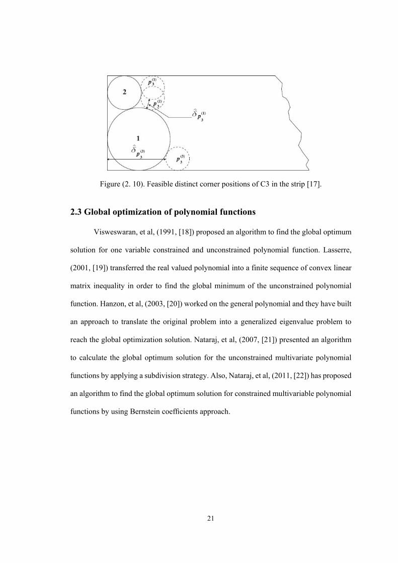
Akeb, et al, (2011, [17]) discussed the circular open dimension problem (CODP)
which is one of the circle packing family problems. They were given a strip of fixed width
and unlimited length, as well as a finite set of n circular pieces of known radii. Their
objective was to search for a global optimum length. They used the minimum local distance
position (MLDP) algorithm for solving the CODP, which was equivalent to the MHD
method as shown in Fig. (2.10).
21
Figure (2. 10). Feasible distinct corner positions of C3 in the strip [17].
2.3 Global optimization of polynomial functions
Visweswaran, et al, (1991, [18]) proposed an algorithm to find the global optimum
solution for one variable constrained and unconstrained polynomial function. Lasserre,
(2001, [19]) transferred the real valued polynomial into a finite sequence of convex linear
matrix inequality in order to find the global minimum of the unconstrained polynomial
function. Hanzon, et al, (2003, [20]) worked on the general polynomial and they have built
an approach to translate the original problem into a generalized eigenvalue problem to
reach the global optimization solution. Nataraj, et al, (2007, [21]) presented an algorithm
to calculate the global optimum solution for the unconstrained multivariate polynomial
functions by applying a subdivision strategy. Also, Nataraj, et al, (2011, [22]) has proposed
an algorithm to find the global optimum solution for constrained multivariable polynomial
functions by using Bernstein coefficients approach.
22
2.4 Clustering techniques
Most of the clustering algorithms required the number of clusters’ centers and their
initial values. The Fuzzy C-Means and k-means algorithms are clear examples of these
types of clustering algorithms. So the accuracy of the solution therefore depends mainly on
the number of cluster centers and their initial values. The mountain method was presented
by Yager, et al, (1994, [23]) as an efficient algorithm to solve the problem of finding the
number of clusters through calculating the number and initial values of the cluster centers.
This algorithm was initiated by gridding the data space and calculating a weight value for
each grid point according to how close it is to the original data points. The grid point’s
weight increases by increasing the number of the close original data points. The highest
weight value grid point will be selected as the first cluster center. Consequently since the
first cluster center is located, the weight values of all grid points are reassigned depending
on how far they are from the cluster center. The closer grid points have lower weight. The
second cluster center is then chosen at the grid point with the highest remaining weight
value. This process continues till the weight value of all grid points retract under a
threshold. In this method, the computing time increases exponentially with the dimension
of the problem because the mountain function must be calculated at each grid point.
Therefore, a development has been achieved by Chiu, (1994, [24]) to the mountain method;
given the name of subtractive clustering method. By using the data points directly as the
candidates for cluster centers, instead of the grid points used in mountain method, the
computational problem would be solved. The computation time became proportional to the
problem size instead of the problem dimension. Bataineh, et al, (2011, [25]) made a
comparison study for different models generated by using subtractive clustering algorithm
23
and others generated by using fuzzy c-means algorithm and they found that the models
generated from subtractive clustering are usually more accurate than those generated using
FCM algorithm. An algorithm is needed to generate accurate models using FCM while is
not needed in the use of subtractive clustering. Also, they mentioned that FCM gives
different results for different runs. Finally, there conclusion was that the subtractive
algorithm produces consistent results.
24
Chapter 3
Polynomial function global optimization by using
subtractive clustering technique
3.1 Introduction
Polynomial functions come in handy every day in which they have a lot of
applications. People use them in the real world because of their ability to describe curves
and surfaces of various types. For example, roller coaster designers may use polynomials
to describe the curves in their rides. Combinations of polynomial functions are used in
economics to do cost analyses. Polynomials have a great efficiency in modelling different
situations in all types of fields like business’ markets’ modelling, in physics to describe the
trajectory of projectiles, in industry to model physical phenomena or mainly for modeling
the sculptured working surfaces, and curves, which we are interested in.
A new optimization technique is proposed in this chapter to calculate the global
optimal solution for the constrained polynomial function. The main contribution of this
technique is to find the global minimum or maximum with reduced the computing time,
improved accuracy, and avoidance of sticking in the local minimum or maximum. Our
focus will be on the one variable and two variables constrained polynomial functions
because they represent curves and surfaces which are the most used in the industrial field.
Since the one variable equation represents a curve and the two variables equation represents
a surface, the problem can be transferred to a geometrical problem.
25
Our approach depends on recognizing the different features of the curves and
surfaces represented by the constrained polynomial function which contain several local
critical points (minima and maxima). These critical points are represented graphically as
peak and valley points of the convex and concave features respectively. By knowing the
local critical points; one of these points will be assigned as the global critical point. The
feature recognition method divides the curve or surface into specified regions according to
the curvature from convex, concave, plane, and saddle regions (for surfaces). Convex
regions contain the local minima and concave regions contain the local maxima which can
be calculated precisely by our algorithm.
The algorithm starts by patching the entity into many data points. The curvature at
each data point will be calculated. The data points which have the same curvature nature
will be grouped together into convex regions, concave regions, plane regions, and saddle
regions. By clustering the planer projections of data points for each group to the enclosed
clusters we can know the exact number of the clusters inside each region. By finding the
center of each cluster, it will be the nearest point to the exact center point. The exact center
point represents a peak point in case of concave region, and valley point in case of convex
region. To calculate the exact center points, the clusters’ center points will be used as initial
points. Using close by points as initial points to find the exact points will make the search
converge very fast. Using the initial local points in simple local optimizer leads to the exact
local points very quickly. The minimum among the local minima will then be the global
minimum. A comparison has been done on several case studies between the proposed
algorithm and the practical swarm optimization (PSO) technique.
26
3.2 Geometric characterization of objective functions
The polynomial functions can be characterized according to the number of the
variables to one and multi-variables. The polynomial function represents geometrically a
curve in case of one variable function and a surface in case of two variables function.
Consequently the curve and surface features describe the variation of the function.
Recognizing these features guides to the peaks and valleys of the function. The
optimization problem starts by assigning the objective function which is the polynomial
function, and the constraints which are the inequalities bounded the working space.
3.2.1 One variable objective function
The objective function which contains one variable represents a curve. It can be
written as
1
( ) n
f x c x c R
(3.1)
min ( )x R
f f x
(3.2.a)
Such that
a x b (3.2.b)
The optimization process starts by patch the curve to several data points as shown in Fig.
(3.1).
27
Figure (3. 1). Curve patching.
Then at each data point the local curvature is calculated by equation (3.3). The curvature
value at each data point predicts the local geometry shape around this data point and
classifies this point to the proper region by convex, concave, or plan according to table
(3.1). The local curve curvature (k) calculations depend on the first and second derivatives
of the polynomial function as shown in equation (3.3).
3
2 2
( )
1 ( )
f xk
f x
(3.3)
Table (3. 1). The Relation between the geometry shape and curve geometry features.
Curvature (k) Local Shape k = 0 Plane k < 0 Concave k > 0 Convex
28
3.2.2 Dual variables objective function
Dual variables objective function represents a surface. It can be written as
1
( , ) y m n
f x y c x c R
(3.4)
( , )min ( , )x y R
f f x y
(3.5.a)
Such that
a x b
c y d
(3.5.b)
The optimization process starts with patch the surface to several data points Fig. (3.2).
Figure (3. 2). Surface patching.
For calculating the curvature, surface is differed than the curve. In order to describe
the surface from a geometric perspective, two critical surface curvatures must be calculated
29
at each data point: Gaussian curvature and mean curvature. These are enough to predict the
local geometry shape around every data point. According to these curvatures, surface shape
is categorised into four types: convex, concave, plane, and hyperbolic shape. All the points
with the same shape are grouped. Gaussian curvature and mean curvature is calculated by
using the first and second fundamental matrices coefficients of the surface. With the help
of first and second fundamental matrices, Gaussian and mean curvatures can be calculated
by using equations (3.6), (3.7). For Gaussian curvature (K):
2
2
FEG
MLNK
(3.6)
For Mean curvature, H:
2FEG
GL2FMEN
2
1H (3.7)
3.2.2.1 The First Fundamental Matrix of Surface
Usually, surfaces are represented by equations ( , )Z f x y in which x and y are the
planer coordinates, and Z is the position vector T ,, zyx of a point on the surface. The
first fundamental matrix of the surface is given by
E F
F G
Z Z Z Z
x x x y
Z Z Z Z
y x y y
A (3.8)
According to Pythagorean theorem 2 2 2ds dx dy , Fig. (3.3).
30
Figure (3. 3). Pythagorean theory.
Since the surface is wrapped, the modified Pythagorean theorem will be the first
fundamental form as shown in Fig. (3.4). The first fundamental form is the expression for
the arc length of the curve passing through any point on the curve:
2 2 22ds Edx Fdxdy Gdy (3.9.a)
since
2z
Ex
z zF
x y
2
zG
y
(3.9.b)
E, F, and G … The coefficients of the first fundamental form of the surface.
31
Figure (3. 4) Modified Pythagorean theory.
3.2.2.2 The Second Fundamental Matrix of Surface
Assuming the existence of the second order derivatives of the surface equations, the
unit normal of a data point is obtained by
Z Zx y
Z Zx y
n the second fundamental matrix is
given by
2 2
2
2 2
2
L M
M N
Z Z
x x y
Z Z
y x y
n n
B
n n
(3.10.a)
since
2
2
zL n
x
2zM n
x y
2
2
zN n
y
(3.10.b)
L, M, and N … The coefficients of the second fundamental form of the surface.
32
3.2.2.3 Surface Geometric Features
By considering the Gaussian and mean curvatures at each data point, the local
geometric shape around the data point can be identified as shown in Fig. (3.5), the criteria
are listed in table (3.2).
Figure (3. 5). Surface shapes according to Gaussian and mean curvature.
Table (3. 2). The Relation among the geometry shape and surface geometry features.
Gaussian Curvature (K) Mean Curvature (H) Point Feature Local Shape
K = 0 H = 0 Parabolic Plane
K = 0 H > 0 Parabolic Concave Cylinder
K = 0 H < 0 Parabolic Convex Cylinder
K > 0 H > 0 Elliptic Concave Ellipse
K > 0 H < 0 Elliptic Convex Ellipse
K < 0 H > 0 or H < 0 Hyperbolic Saddle
33
3.3 Clustering technique
After recognizing the curvature at each data point for both the curve and the surface,
the points which have the same curvature type will be grouped. The entity may contains
one or more regions inside each group, for each region, it must contains one of the critical
points. The next step is to then find the number of these regions inside each group, and the
center of each region which represents one of the local critical points, for doing so the
subtractive clustering technique is adopted. Clustering is the process of grouping a set of
elements into the same group or cluster so that elements in the same group are to somehow
similar or have common factor. According to the elements, distribution, and the objective
of the clustering, different types of similarities are used to place elements into groups,
where the similarity value controls how the clusters are shaped. Some examples of these
types of similarities are distance, and intensity.
There are two main types of clustering; the hard clustering, and the soft clustering.
In hard clustering, elements are divided into discrete clusters, where each element belongs
to a single exact cluster. In soft clustering, the elements can have relationships with certain
levels to more than one cluster, the relationships levels are attached to each element. The
relationships levels for each element refer to how strong the bond is between the element
and a particular cluster. Subtractive clustering is one of the processes to designate the
relationships levels, consequently using these levels to assign the elements to one or more
clusters.
34
3.3.1 Subtractive clustering method
Most of the clustering algorithms required the number of clusters’ centers and their
initial values. The Fuzzy C-Means and k-means algorithms are clear examples of these
types of clustering algorithms. So the accuracy of the solution therefore depends mainly on
the number of cluster centers and their initial values. Based on the literature review, we
used the Subtractive Clustering Method to calculate the number of the clusters and the
clusters’ centers. The subtractive clustering method assumes that each data point is a
potential cluster center. A data point with more neighboring data will have a higher
opportunity to become a cluster center than points with fewer neighboring data. For
subtractive clustering of a group of data points {x1, x2… xn}; the method starts by
considering each data point as a potential cluster center.
a. Initial potentials of the point set
At first, each data point is regarded as a potential cluster centre, and each cluster has
only one data point as the centre itself. The potential of a data point, ix , is defined by
nin
ji
ji ,...,2,1 ,eP1
2
xx
(3.11.a)
where
2
4
ar
(3.11.b)
and ar is a positive constant. The potential of a data point is a function of the distances
between this point, and every other point. The shorter is the distance, the more contribution
to the summation. For a data point in dense area, its potential is higher than that in sparse
35
area. Usually, the distance is in the metric of Euclidean norm that is the sum of the squares
of the difference in each dimension. In order to consider the importance variation of
dimensions, different weights are assigned to different dimensions. Therefore, the distance
can be calculated by:
21,1,12
3,3,212 ... pjpipjiji xxwxxwswxx
(3.12)
The constant, ar , is the radius defining the neighborhood of a data point: data points inside
the circle produce significant potential for the centric data point, and data points outside
exert little influence on the potential.
b. Choose the first cluster center and update the potentials
The data point with highest potential is selected as the first cluster center. The
reason is that this point is closely surrounded by a maximum number of data points. The
maximum potential 1
Pc of the first cluster center 1cx is:
n
jn
jc
121c
2
1
1eP,...,P, PmaxP
xx(3.13)
The potential of each data point is then revised by the formula
niic
ii ,...,2,1 ,ePPP2
1
1c xx (3.14.a)
where
2
4
br (3.14.b)
and br is a positive constant. The subtractive amount from the potential of each point is
nonlinear, and inversely proportional to the distance between the point and the first cluster
center. Therefore, the potentials of data points closer to the first cluster center are reduced
36
to a very small number, and the potential of the first cluster center becomes null at last. On
the contrary, the point far away from the center has larger potential comparatively. The
purpose of subtraction is to find the second cluster center farther away from the first one.
The constant, br , is also a radius defining a circular region, and the point will have
measurable reduction in potential, if contained in the region. Usually, br is set to be greater
than ar .
c. Choose the second cluster centre
Among the updated potentials of data points, the data point with the highest
potential is selected as the second cluster center.
n
jn
jc
1
21c
2
2
2e P,...,P, PmaxP
xx(3.15)
Same as the previous step, part of the highest potential of the second cluster center is
subtracted from the potential of every data point. In general, if the kth cluster center is
found, the potential modification is carried out using the formula
niikc
ii ,...,2,1 ,ePPP2
k
c
xx (3.16)
This process will create a series of cluster centers, 1 2, , ...,
kc c cx x x .
d. The criteria for accepting and rejecting cluster centers
If k 1c cP P , the data point
kcx will be accepted as a cluster center and continue. But if
k 1c cP P , the data point kcx will be rejected and the clustering process will be seized. The shortest
distance among all the distances between kcx and cluster centers will be set as mind . In case the
stopping criteria was not satisfactory:
37
k
1
cmin
c
Pd1
Par (3.17)
Again kcx will be accepted as the new cluster center, and the algorithm will continue, otherwise
the new cluster center kcx will be rejected and the potential of
kcx will be set as zero. This process
will be repeated till the stopping criteria is satisfied. The two constants are set as,
0.5, and 0.15 .Through the subtractive process, the number of clusters, and their centers
are found.
3.4 Optimization technique
The approach objective is to calculate the global optimum by finding all the available local
minima. According to these objective, the optimization procedures are consist of three steps.
3.4.1 Patching
The first step starts with calculating several data points on the surface or the curve
represented by the objective function. The selected data points have the same infinitesimal
distances and areas between each other, this process is called patching. The selected data points
will be the input points to our algorithm. By testing the curvature for each data point (Gaussian and
main curvatures in case of the surface, and the local curvature in case of the curve) these points can
be classified into different groups according to the curvature values at each point. These groups are
convex, concave, plane, and saddle (in case of the surface) groups. According to the type of the
optimization process, whether it is minimization or maximization, the working group will be
assigned. The convex group will be the working group in case of minimization, and the concave
group will be the working group in case of maximization.
38
3.4.2 Clustering
The working group data points will then be the input for the second step which is the
clustering process. The subtractive clustering process is the candidate process to be applied in this
algorithm because of the pre-mentioned advantages. Subtractive clustering process is looking for
the clusters’ centers of the input working group data points. According to the intensity distribution
of the data points in the working group, the number of clusters’ centers and their locations will be
assigned. The clusters’ center points are from the input data points. The main reason of applying
the clustering process is to find the closest points to the real center points of the peaks or the valleys
of the tested surface or curve which represented by the objective function, therefore the clusters
centers are the closest points to the real center points of the peaks or the valleys. To find the real
center points of the peaks or the valleys another step should be carried out.
3.4.3 Local optimization
The local optimization methods have some merits compared with the global optimization
methods. The local optimization methods tend to converge very quickly whereas, global methods
might take time. Also, the accuracy of the local optimization methods to discover the solution is
much better than the accuracy of the global optimization methods, therefore the global optimization
methods having many parameters must be tuned to improve the accuracy of finding the final
solution. From everything mentioned above, it is concluded that; if the local optimization method
is adapted to discover the global solution of multiple local minima and maxima functions it will be
faster and more accurate.
Thereby we Quasi Newton method in our algorithm to ensures the high accuracy and low
computational time. The Quasi-Newton method is one of the most famous algorithms for finding
the local maxima or minima of the objective functions. Quasi-Newton method is based on Newton's
method to find the stationary point of the objective function, where the gradient is 0. Newton's
39
method uses the first and second derivatives to find the stationary point staring from an initial point.
The closer the initial point from the stationary point, the faster the solution is reached. By using the
clusters centers that we obtain from the clustering algorithm as initial points for the Quasi-Newton
method ensures a fast convergence in the optimization process. After calculating all the local
optimum points, the global optimum point is one of them.
3.5 Applications
To verify the validity of our new approach, different case studies are tested. The cases are
divided according to the number of variables; one variable and two variables objective
functions. Different objective functions with different numbers of the local minima are
used.
3.5.1 One variable objective function case studies
3.5.1.1 Case study I
In the first case study the objective function as shown in equation (3.18.a), with the
constraint inequality equation (3.18.b). Fig. (3.6.a) shows the data points coming from gridding the
objective function. By checking the data points, they are grouped into two groups as shown in Fig.
(3.6.b).
4 3 2( ) 3 9 23 12f x x x x x (3.18.a)
Such that
4.5 4.5x (3.18.b)
40
(a) First case study data points.
(b) Data points groups (Convex group “ . ”, Concave group “ * )
-5 -4 -3 -2 -1 0 1 2 3 4 5-100
-50
0
50
100
150
200
250
300
350
400
-5 -4 -3 -2 -1 0 1 2 3 4 5-100
-50
0
50
100
150
200
250
300
350
400
41
For a minimization problem the convex group is selected. By applying the subtractive
clustering technique the number of clusters with the clusters’ centers are calculated as
shown in Fig. (3.6.c). The clustering technique gives two clusters with two centers as
shown in table (3.3).
(c) The center point of each cluster “*”, and the global minimum point “●”.
Figure (3. 6). Curve first case study.
Table (3. 3). Case study I clusters centers.
x F(x)
1 -3 -24
2 2 -54
-5 -4 -3 -2 -1 0 1 2 3 4 5-100
-50
0
50
100
150
200
250
300
350
400
42
Using the clusters’ centers as initial points in Quasi-Newton algorithm, the exact local
minima is calculated as illustrated in table (3.4).
Table (3. 4). Case study I exact local minima.
x f(x)
1 -3.103 -24.211 2 1.853 -54.644
The smaller value of the f(x) represents the global minimum of the objective function as
shown in table (3.4).
3.5.1.2 Case study II
6 5 4 3 21 1 7 3( ) 2 2 2
8 4 8 2f x x x x x x x (3.19.a)
Such that
2.5 2.5x (3.19.b)
(a) Second case study data points.
-3 -2 -1 0 1 2 3-3
-2
-1
0
1
2
3
43
(b) Data points groups (Convex group “ . ”, Concave group “ * ” )
For a minimization problem the convex group is selected. By applying the subtractive
clustering technique, the number of clusters with the clusters’ centers are calculated as
shown in Fig. (3.7.c). The clustering technique gives three clusters with three centers as
shown in table (3.5).
-3 -2 -1 0 1 2 3-3
-2
-1
0
1
2
3
44
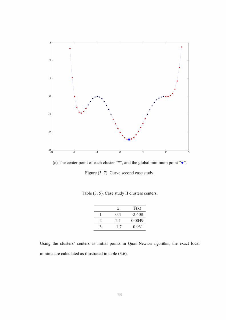
(c) The center point of each cluster “*”, and the global minimum point “●”.
Figure (3. 7). Curve second case study.
Table (3. 5). Case study II clusters centers.
x F(x)
1 0.4 -2.408 2 2.1 0.0049
3 -1.7 -0.931
Using the clusters’ centers as initial points in Quasi-Newton algorithm, the exact local
minima are calculated as illustrated in table (3.6).
-3 -2 -1 0 1 2 3-3
-2
-1
0
1
2
3
45
Table (3. 6) Case study II exact local minima.
x f(x) 1 0.387 -2.409 2 2.07 0.003
3 -1.721 -0.934
The smaller value of the f(x) represents the global minimum of the objective function as
shown in table (3.6).
3.5.1.3 Case study III
5 4 3 2( ) 4 8 5 10 2f x x x x x x (3.20.a)
Such that
1.5 2.5x (3.20.b)
(a) Third case study data points.
-1.5 -1 -0.5 0 0.5 1 1.5 2 2.5-6
-4
-2
0
2
4
6
46
(b) Data points groups (Convex group “ . ”, Concave group “ * ” )
By applying the subtractive clustering technique to the convex group as a minimization
problem, the number of clusters with the clusters’ centers are calculated as shown in Fig.
(3.8.c). The clustering technique, gives two clusters with two centers as shown in table
(3.7).
-1.5 -1 -0.5 0 0.5 1 1.5 2 2.5-6
-4
-2
0
2
4
6
47
(c) The center point of each cluster “*”, and the global minimum point “●”.
Figure (3. 8). Curve third case study.
Table (3. 7). Case study III clusters centers.
x F(x)
1 -0.05 -2.024
2 1.65 -5.963
Using the clusters’ centers as initial points in Quasi-Newton algorithm, the exact local
minima are calculated as illustrated in table (3.8).
Table (3. 8). Case study III exact local minima.
x f(x) 1 -0.048 -2.024
2 1.681 -6.007
-1.5 -1 -0.5 0 0.5 1 1.5 2 2.5-8
-6
-4
-2
0
2
4
6
48
The smaller value of the f(x) represents the global minimum of the objective function as
shown in table (3.8).
3.5.1.4 Case study IV
8 7 6 5 4 3 2( ) 4 12 3 4 7 20 12f x x x x x x x x x (3.21.a)
Such that
1.5 3x (3.21.b)
(a) Fourth case study data points.
-1.5 -1 -0.5 0 0.5 1 1.5 2 2.5 3-70
-60
-50
-40
-30
-20
-10
0
10
20
30
49
(b) Data points groups (Convex group “ . ”, Concave group “ *” )
To solve the minimization problem the convex group is selected. By applying the
subtractive clustering technique, the number of clusters with the clusters’ centers are
calculated as shown in Fig. (3.9.c). The clustering technique gives three clusters with three
centers as shown in table (3.9).
-1.5 -1 -0.5 0 0.5 1 1.5 2 2.5 3-70
-60
-50
-40
-30
-20
-10
0
10
20
30
50
(c) The center point of each cluster “*”, and the global minimum point “●”.
Figure (3. 9). Curve fourth case study.
Table (3. 9). Case study IV clusters centers.
x F(x)
1 -1.1 0.087
2 1 -32 3 2.8 -62.089
Using the clusters’ centers as initial points in Quasi-Newton algorithm, the exact local
minima are calculated as illustrated in table (3.10).
-1.5 -1 -0.5 0 0.5 1 1.5 2 2.5 3-70
-60
-50
-40
-30
-20
-10
0
10
20
30
51
Table (3. 10). Case study IV exact local minima.
x f(x)
1 -0.998 0.004 2 1 -32 3 2.755 -63.516
The smaller value of the f(x) represents the global minimum of the objective function as
shown in table (3.10).
3.5.2 Two variables objective function case studies
3.5.2.1 Case study I
In the first case study, the objective function as shown in equation (3.22.a), and the working
space constraints are the variables boundaries as inequality constraints. Fig. (3.10.a) shows the data
points coming from gridding the objective function. By testing the data points’ curvature, they are
grouped into four groups as shown in Fig. (3.10.b).
2 21 1( 2 )/1000
2 21( , )
3
x y y
f x y xye (3.22.a)
Such that
100 100
100 100
x
y
(3.22.b)
52
(a) First case study data points.
(b) Data points groups (Convex group “ . ”, Concave group “ * ”, hyperbolic group “ o ”,
and plane group “ x ”).
53
For a minimization problem the convex group is selected. By applying the subtractive
clustering technique, the number of clusters with the clusters’ centers are calculated as
shown in Fig. (3.10.c). The clustering technique gives two clusters with two centers as
shown in table (3.11).
(c). Convex data points clusters with the clusters centers “□” and the global minimum
point “●’
Figure (3. 10). Surface first case study.
Table (3. 11). Case study I clusters centers.
x y
1 14 -31 2 -16 29
Using the clusters centers as initial points in Quasi-Newton algorithm, the exact local minima
are calculated as illustrated in table (3.12).
-30 -20 -10 0 10 20 30-60
-40
-20
0
20
40
60
54
Table (3. 12). Case study I exact local minima.
x y f(x,y)
1 15.8114 -31.8738 -62.3552 2 -15.8114 31.8738 -62.2943
The smaller value of the f(x,y) represents the global minimum of the objective function as
shown in table (3.12).
3.5.2.2 Case study II
The objective function
2 2 2 2 2 22 ( 1) 3 5 ( 1)( , ) 3(1 ) (2 10 10 ) 0.3x y x y x yf x y x e x x y e e (3.23.a)
Such that
3.5 3.5
3.5 3.5
x
y
(3.23.b)
(a) Second case study data points.
55
(b) Data points groups (Convex group “ . ”, Concave group “ * ”, hyperbolic group “ o ”,
and plane group “ x ”).
For solving the minimization problem the convex group is selected. By applying the
subtractive clustering technique, the number of clusters with the clusters’ centers are
calculated as shown in Fig. (3.11.c). The clustering technique gives four clusters with four
centers as shown in table (3.13).
56
(c) Convex data points clusters “.” with the clusters centers “□” and the global minimum point “●”
Figure (3. 11). Surface second case study.
Table (3. 13). Case study II clusters centers.
x y
1 0.2 -1.6
2 -1.3 0.2 3 2 1.3 4 0.3 0.4
Using the clusters’ centers as initial points in Quasi-Newton algorithm, the exact local
minima are calculated as illustrated in table (3.14).
-2 -1.5 -1 -0.5 0 0.5 1 1.5 2 2.5 3-2.5
-2
-1.5
-1
-0.5
0
0.5
1
1.5
2
57
Table (3. 14). Case study II exact local minima.
x y f(x,y) 1 0.2283 -1.6255 -6.511
2 -1.3474 0.2045 -3.0498
3 4.1981 2.2898 0
4 0.2964 0.3202 -0.0649
The smaller value of the f(x,y) represents the global minimum of the objective function as
shown in table (3.14).
3.5.2.3 Case study III
The objective function
2 4 6 2 41( , ) 4 2 4 4
3f x y x x x xy y y (3.24.a)
Such that
2 2
1 1
x
y
(3.24.b)
(a) Third case study data points.
58
(b) Data points groups (Convex group “ . ”, Concave group “ * ”, hyperbolic group “ o ”,
and plane group “ x ”).
To calculate the global minimum, the convex group is selected. By applying the subtractive
clustering technique, the number of clusters with the clusters’ centers are calculated as
shown in Fig. (3.12.c). The clustering technique gives six clusters with six centers as shown
in table (3.15).
-2 -1.5 -1 -0.5 0 0.5 1 1.5 2-1
-0.8
-0.6
-0.4
-0.2
0
0.2
0.4
0.6
0.8
1
59
(c) Convex data points clusters “.” with the clusters centers “□” and the global minimum point “●”
Figure (3. 12). Surface third case study.
Table (3. 15). Case study III clusters centers.
x y
1 0 0.8
2 0 -0.8
3 1.7 0.8
4 -1.7 0.8
5 1.7 -0.8
6 -1.7 -0.8
-2 -1.5 -1 -0.5 0 0.5 1 1.5 2-1
-0.8
-0.6
-0.4
-0.2
0
0.2
0.4
0.6
0.8
1
60
Using the clusters’ centers as initial points in Quasi-Newton algorithm the exact local minima
are calculated as illustrated in table (3.16).
Table (3. 16). Case study III exact local minima.
x y f(x,y) 1 -0.089 0.712 -1.031
2 -0.089 -0.712 -0.903
3 1.703 0.796 -0.215
4 -1.703 0.796 -0.215
5 1.703 -0.796 -0.215
6 -1.703 -0.796 -0.215
The smaller value of the f(x,y) represents the global minimum of the objective function as
shown in table (3.16).
3.5.2.4 Case study IV
The objective function
30x( , ) 5sin( )sin( )e
30 30
xyf x y
(3.25.a)
Such that
60 60
60 60
x
y
(3.25.b)
61
(a) Fourth case study data points.
(b) Data points groups (Convex group “ . ”, Concave group “ * ”, hyperbolic group “ o ”,
and plane group “ x ”).
-60 -40 -20 0 20 40 60-60
-40
-20
0
20
40
60
62
Similar to the previous case studies, for solving the minimization problem the convex
group is selected. By applying the subtractive clustering technique, the number of clusters
with the clusters’ centers are calculated as shown in Fig. (3.13.c). The clustering technique
gives eight clusters with eight centers as shown in table (3.17).
(c) Convex data points clusters “.” with the clusters centers “□” and the global minimum point “●”
Figure (3. 13). Surface fourth case study.
-60 -40 -20 0 20 40 60-60
-40
-20
0
20
40
60
63
Table (3. 17). Case study III clusters centers.
x y
1 18 -15
2 -12 15
3 18 45
4 -12 -45
5 48 15
6 48 -45
7 -42 -15
8 -42 45
Using the clusters’ centers as initial points in Quasi-Newton algorithm, the exact local
minima are calculated as illustrated in table (3.18).
Table (3. 18). Case study III exact local minima.
x y f(x,y) 1 17.942 -14.99 -8.664
2 -12.057 14.99 -3.187
3 17.942 44.99 -8.664
4 -12.057 -44.99 -3.187
5 47.942 14.99 -23.553
6 47.942 -44.99 -23.553
7 -42.057 -14.99 -1.172
8 -42.057 44.99 -1.172
The smaller value of the f(x,y) represents the global minimum of the objective function. In
this case, the algorithm gives two locations for the same value global minimum which
cannot be detected by any other algorithms.
64
3.5.3 Comparison between our approach and PSO
The pre-mentioned case studies are solved by using the particle swarm optimization
(PSO) algorithm in order to make a comparison with the results obtained by using our
approach, as shown in table (3.19).
Table (3. 19). Comparison between our approach and PSO
One variable objective functions The new approach PSO
x - f(x) Time (sec)
x - f(x)
Time (sec)
Time saved
1 1.853 - -54.644 1.012 1.853 - -54.644 2.023 50 %
2 0.387 - -2.409 0.987 0.387 - -2.409 1.619 39 % 3 1.681 - -6.007 1.186 0 - 0 0.88 - 4 2.755 - -63.516 1.278 2.755 - -63.516 2.697 52.6 %
Two variables objective functions
x y f(x,y) Time (sec)
x y f(x,y)
Time (sec)
Time saved
1 -15.8114 31.8738 -62.2943 1.1447 -6 6 -11.001 0.784 -
2 0.2283 -1.6255 -6.511 1.2415 0.2828 -1.5784 -6.499 3.8226 67.5 % 3 -0.089 0.712 -1.031 1.2376 0.089 -0.7127 -1.031 2.8393 56.4 % 4 47.942 14.99 -23.553 1.2654 6 -6 -2.1099 0.829 -
From the table (3.19), it is clear that by using the new approach there is a time saving of
about 50 %. Also, in some cases, the PSO algorithm gets stuck in local minimum. In the
PSO algorithm, each run leads to a different solution.
3.6 Conclusion
A new global optimization algorithm is proposed to solve polynomial functions of
one, or two variables by using the subtractive clustering technique. The new proposed
65
algorithm proves to be successful in finding the global solution for polynomial functions
with one, or two variables. The results obtained from comparing the new approach with
the particle swarm optimization algorithm on several case studies showed that the new
approach is faster by about two times, with a very good repeatability, and has a great
capability to avoid getting stuck in the local minimum.
66
Chapter 4
Plunge milling tool path optimization
4.1 Introduction
From the literature review; it is found that the proper cutting forces and tool path
planning are important elements to improve the efficiency of the plunge milling process.
Therefore our focus will be on improving the efficiency of plunge milling process by
maximizing the removed material using the least number of plunging points. This will
strongly reduce the total machining time, in addition to optimizing each tool path by
solving the travelling salesman problem (TSP) through the use of the simulated annealing
optimization technique while taking into consideration a very important aspect which is
the tool availability.
In this chapter, the 2D pocket with polygon boundary area is covered with specified
radii circles in two steps. (1) Fill the pocket with the minimum number of specified radii
circles which are tangent to each other and/or the pocket boundary without overlapping by
building an algorithm using the maximum hole degree (MHD) theory for solving the circle
packing problem. (2) Cover the areas left between the non-overlapped circles by using the
same specified radii. After obtaining the circle loci, the circles are grouped according to
the radii. The tool path for each group is optimized by solving the travelling salesman
problem (TSP) using the simulated annealing (SA) technique. By the end of this chapter,
67
the model will be applied on a free-form pocket boundary with an island, and sculptured
surface bottom.
4.2 Circle packing mathematical model
From geometry point of view, circle packing is the circles arrangement study (equal
or different sizes) on a given plain surface such that no overlapping occurs, and all circles
touch each other. According to literature, the maximum hole degree method is one of the
most used methods for packing non-overlapped circles inside a specified boundary.
Therefore, the maximum hole degree method is adopted in our work.
The mathematical model consists mainly of two algorithms. (1) Algorithm for
filling a pocket with non-overlapping circles of specified radii by applying the maximum
hole degree method to solve the non-overlapped circle packing problem. (2) Algorithm for
covering the gaps between the non-overlapped circles coming from the first algorithm to
maintain the complete covering of the surface area with the same specified radii circles.
4.2.1 Maximum hole degree theory
Inspired from human experience in packing, the benefits of placing an object at
different positions in a container are different. This can be represented by a Chinese
proverb; “Gold corner, silver side, and grass middle”. It means that for packing places
inside a container the corner positions possess higher values than those at the side while
the side positions possess higher values than those in the middle. From the previous
discussion, for each position of the circle to be placed, there is a parameter represents the
benefit of this position to the hole packing configuration. This parameter is called the hole
68
degree, in which corners have the highest hole degree which is called corner placement.
Therefore, placing circles at corner positions leads to better packing configuration. The
word corner is not just the region between two of the container’s boundaries but also the
region formed by two circles already placed inside the container, or a circle and any of the
container boundaries. With regard to applying this theory on the practical case studies, an
algorithm is built.
4.2.2 Algorithm to fill a pocket with tangent circles of specified radii
The packing problem is concerned with how to pack objects with a given shape, and
size, into a bounded space without overlap. Filling the pocket area with circles of specified
radii has been done in several steps according to the flow chart Fig. (4.1). The main
procedure is filling the pocket with the specified circles in decreasing order, where they are
tangent to the existing circles and/or the pocket polygon. These steps are repeated until
there is no more space is available for any of the specified circles. The decreasing order is
used with regard to the plunging application. Using the bigger diameters as much as we
can reduces the number of plunging places which by rule reduces the machining time.
69
Tools radii Pocket verixes
First circle
Second circle
Add to circles matrix
Gauge and overlap
Select the smaller radius
Last available
radius
Yes
No
Yes
Calculate the hole degree per each
No
Find all feasible corner placements
Select the one with max hole degree
GaugeSelect the
smaller radius
End
Yes
Yes
Convexity
Add to circles matrix
No
Last available
radiusNo
Figure (4. 1). First algorithm flow chart
70
4.2.2.1 Check convexity of the polygon corners
The polygon corners must be checked to know whether they are convex or concave.
The convex corner is one of the candidate corner placements. The given is a polygon with
its vertices ordered in a counter clock wise manner. The polygon vertices are
ip i 1 , 2, , n as shown in Fig. (4.2). For any two edges i i 1 i 1 i 2p p ,p p
since they are in
xy plane, the cross product of the two edges gives the value and direction of the
perpendicular in the z coordinate according to the right hand rule as shown in Fig. (4.2).
i 1i i 1 i 1 i 2
i 1
z Convex at p cornerp p p p
z Concave at p corner
(4.1)
p1 p2
pi
pi+1
pn
pi+2pi+3
pipi+1 pi+1pi+2
pi+1pi+2 pi+2pi+3
Figure (4. 2). Convexity check. 4.2.2.2 Check boundaries gauging
Gauging is not allowed in this algorithm. So, the current circle is checked for
intersection with the polygon, if the intersection exists, the plunger will gauge the part. A
71
polygon with vertices pi (i = 1, 2… n) and a circle with center O and radius R are shown in
Fig. (4.3). The coordinates of ii
i
xp
y
, and the coordinates of x
y
OO
O
. In general, the
parametric equation of i i 1p p
will be:
i i 1 i i 1 ip u p p p u p - p
(4.2)
pi
pi+1
pper
o
R
D
Figure (4. 3). Boundaries gauge check.
per i i 1p O p p 0
(4.3)
Substituting in (4.3) with (4.2)
per i 1 iO p p p 0 (4.4)
per i i 1 ip p u p - p (4.5)
i i 1 i i 1 iO p u p p p p 0 (4.6)
72
i i 1 i i 1 iO p u p p p p 0 (4.7)
i i 1 i i 1 i i 1 iO p p p u p p p p 0 (4.8)
2
i i 1 i i 1 iO p p p u p p 0
(4.9)
The u value corresponding to the point pper can be calculated as:
x 1 2 1 y 1 2 1
per 2
2 1
o x x x o y y yu
p p
(4.10)
perp 1 per 2 1x x u x x (4.11)
perp 1 per 2 1y y u y y (4.12)
The perpendicular distance from the center to i i 1p p
perD p O
(4.13)
Then gauging VG depends on (u, D)
G
0 u 0,1 , D RV
1 u 0,1 , D R
(4.14)
In some cases (concave corners) the perpendicular distance is less than the circle’s radius
but there is no gauging as shown in Fig. (4.4). The general form will then be:
73
Gi i 1
i i 1
0 u 0,1 ,D R
1 u 0,1 ,D RV
0 u 0,1 , Op R and Op R
1 u 0,1 , Op R or Op R
(4.15)
pi
pi+1
pper
o
R
Figure (4. 4). General case.
4.2.2.3 Check circles overlap
The current circle is checked for intersection with any other circle inside the
polygon. For two circles with centers O1, O2 and radii R1, R2, the center distance (D) must
be checked as shown in Fig. (4.5)
1 2D O O
(4.16)
Then intersection Vint depends on the value of (D)
1 2int
1 2
0 D R RV
1 D R R
(4.17)
74
o2o1
o2o1
D
D
Intersection = 0
Intersection = 1
R1R2
Figure (4. 5). Circles overlapping check.
4.2.2.4 Calculate the corner placements
According to the previous researches in circle packing, the corners are the best
places to be packed because they give a very close packing arrangement which enable more
items to be packed. The corner placement can be defined as a placement pcpj of a given
circle j with center point coordinates xj , yj , and radius rj , is considered feasible if the circle
lies completely inside the polygon (no gauging with the boundaries). A feasible placement
is called a corner placement if the circle touches two items at least (i.e. two polygon edges,
edge and circle or two other circles). The available corner placements to the next circle will
be calculated in two cases: Case A: The current circle is tangent to one or more of the
polygon edges, as shown in Fig. (4.6). Case B: The current circle is tangent to one or more
of the existing circles inside the polygon, as shown in Fig. (4.7). In both cases it is given:
75
(1) Polygon with its vertices. (2) Circle with its location inside the polygon and its radius.
(3) The radii of the circles to be packed.
Case (A):
To calculate the available corner placement center (pcp) in case of the current circle
being tangent to one or more of the polygon sides, the polygon with its vertices are pi (i =
1, 2… n) and a circle with center O and radius R, as shown in Fig. (4.6).
R
rj
Pi
Pi+1
Pioff
PCP
Pi-1
Pi+2
Pi+1off
o
Ø
PQ
x
Figure (4. 6). Corner placements for a circle tangent to a boundary.
76
The coordinates of ii
i
xp
y
, and the coordinates ofx
y
OO
O
. The next circle will be with
center j
j
xC
y
, and radius rj. In general, vector i i 1p p
will be taken as an example. Two
steps are required to calculate (pcp):
(1) Calculate the offset points ( io ff i 1offp , p ) of the start and end points i i 1p , p inside the
polygon:
a. Calculate the angle () between i i 1p p
, and i 1 ip p
i 1 i i i 1 i 1 i i i 1p p . p p p p p p cos
(4.18)
1 i 1 i i i 1
i 1 i i i 1
p p . p pcos
p p p p
(4.19)
b. Calculate the angle () between i i 1p p
and positive x-axis
i 1 i i i 1x x p p cos 0 2
(4.20)
i 1 i i i 1y y p p sin
(4.21)
1 i 1 i
i i 1
x xcos
p p
(4.22)
The offset point of (pi) w.r.t the next circle with radius rj will be (pioff)
The polar angle of i ioffp p
77
2
θ (4.23)
ji ioff
rp p
sin2
(4.24)
ioff i i ioffx x p p cos
(4.25)
ioff i i ioffy y p p sin
(4.26)
2. Calculate the corner placement center point w.r.t the radius of the next circle (rj):
After offsetting the line i i 1p p
by the value rj inside the polygon, we get the line
ioff i 1offp p
. By offsetting the circle with center O and radius R in order to have same center
and radius equal to (R+rj). The corner placement center points will be the intersection
points between the offset circle and the line ioff i 1offp p
. To calculate the intersection points
the equation ioff i 1offp p
will be
ioff i 1off ioff i 1off ioffQ p p p v p p 0 v 1
(4.27)
The dot product of the line Qp O
, and ioff i 1offp p
which are perpendicular to each other
at Qp 0 .
i 1off ioffO Q p p 0 (4.28)
Plugging equation (4.27) in (4.28):
ioff i 1off ioff i 1off ioffO p v p p p p 0 (4.29)
78
The (v) value corresponding to the point ( Q p ) can be calculated as:
x iof i 1off ioff y ioff i 1off ioff
2
i 1off ioff
o x x x o y y yv
p p
(4.30)
Q ioff i 1off ioffx x v x x (4.31)
Q ioff i 1off ioffy y v y y (4.32)
and,
Qd p O
(4.33)
For the triangle O pQ pcp:
cp jp O R r
(4.34)
Q cp cp x x p O .cos . cos
(4.35)
cp Q cp x x p O .cos . cos
(4.17)
Q cp cp y y p O .cos . sin
(4.37)
cp Q cp y y p O .cos . sin
(4.38)
… The angle between cp p O
, and cp Qp p
.
79
Case (B):
To calculate the available corner placements in case of two circles are tangent to
each other, as shown in Fig. (4.7). Two circles with centers (Oi, Oi+1) and radii (Ri+1, Ri)
and center. The coordinates of xi
iyi
OO
O
, and the coordinates of xi 1
i 1yi 1
OO
O
. The next
circle will be with center j
cpj
xp
y
and radius rj. To calculate the coordinates of the point
pcp:
1. Get the offset circle from the first circle by the value of rj, the resultant circle will be
with the same center Oi and radius i jR r .
2. Get the offset circle from the second circle by the value of rj, the resultant circle will
have the same center Oi+1 and radius i 1 jR r .
3. The intersection points between the resultant two offset circles will be the available
corner placements centers to the next circle which can be calculated as follow:
i. Get the cosine value of the angle between i i 1O O
and i cpO p
:
i i 1 i i 1O O R R
(4.39)
i 1 cp i 1 jO p R r
(4.40)
cp i j ip O r R
(4.41)
80
Oi Oi+1
pcp
Ri+1
Ri
I
rj
Figure (4. 7). Corner placements with other circles.
2 2 2
i i 1 i cp cp i 1
i i 1 i cp
O O O p p O cos
2 O O O p
(4.42)
ii. Calculate the unit vector for line i i 1O O
denoted by U
i 1 i
i i 1
O OU
Oˆ
O
(4.43)
x
y
ˆ UU
U
(4.44)
Calculate iO I
i i cpO I O p cos
(4.45)
81
From Fig. (4.7)
i cp j iO p r R
(4.46)
i j iO I r R cos
(4.47)
i j iO I U r R coˆ s
(4.48)
iii. Calculate the unit perpendicular vector for line i i 1O O
:
yper
x
UU
Uˆ
(4.49)
iv. Calculate the vector cpIp
cp i cpIp O p sin
(4.50)
2cp j iIp r R 1 cos
(4.51)
2cp per j iIp U r sˆ R 1 co
(4.52)
The intersection point cpp can be calculated
cp i i cpp O O I Ip
(4.53)
2cp i j i per j ip O U r R cos U r R 1 cos (4.54)
4.2.2.5 Corner placements feasibility check
The corner placement is said to be feasible if it exists inside the polygon, and the
circle with the center of this corner placement must at least touch two items inside the
82
polygon without intersection with any other item. To check the feasibility for the corner
placement, two tests must be applied:
(a) Inside-polygon check.
(b) Circles intersection check. Given:
1. For each tangent circle and boundary there exist two corner placements.
2. For each two tangent circles there exist two corner placements.
According to the definition of the corner placement a tangency must occur between the
next circle and two items inside the polygon (two circles, circle and boundary, or two
boundaries).
a. The first check, inside-polygon check:
If the corner placement center is inside the polygon this means that the whole next circle
will be inside the polygon according to the tangency condition. To check the corner
placement center j
jj
xC
y
, if inside the polygon or not, the next steps are applied:
1. Obtain the points with the largest x-coordinate ( maxx ) and lowest x-coordinate ( minx )
values among the polygon vertices.
2. Establish a horizontal line with a start, and an end points as:
Start pointmin
sj
xp
y
, End point max
ej
xp
y
The line equation is
s l e sL p u p p (4.55)
The horizontal line will intersect with some of the polygon boundaries.
83
3. Get the intersection points with the polygon boundaries int
intj
xp , int 1,2, ,k
y
k … the number of polygon boundaries.
4. The polygon boundaries general formula is
i i 1 iP p u p p (4.56)
At the intersection points the boundary line equation, and the horizontal line equation are
equal
i i 1 i s l e sp u p p p u p p (4.57)
i i 1 i min l max minx u x x x u x x (4.58)
i i 1 i j l j jy u y y y u y y (4.59)
From (4.59):
j i
i 1 i
y yu
y y
(4.60)
If u 0,1 , Sub with (4.60) in (4.56)
int i i 1 ip p u p p (4.61)
Since all the points have the same yj coordinate
int i i 1 ix x u x x (4.62)
If u 0,1 , there is no intersection between this boundary and the horizontal line.
84
5. After obtaining all values of intx int 1,2, , k :
By excluding the points which have coordinatesj
int i
i
x x
y y
. For the rest of intx
the value of inC will indicate if the circle is inside or outside the polygon according to the
number of intersection points with the polygon boundaries to the right and the left of the
tested point (nr, nl)
r lin
r l
1, n ,n 2n 1C
0, n ,n 2n
n 0,1,2,...
(4.63)
rn Number of points with int jx x (to the right of the tested point)
ln Number of points with int jx x (to the left of the tested point)
Examples are illustrated in Fig. (4.8).
Cj p1pintpk p2
Cj p1pintpk p2
(a)
(b)
Figure (4. 8). Check point inside a polygon.
85
b. The second check, circle overlaps check:
In this algorithm the intersection between circles or a circle encloses by another
circle is not allowed as shown in Fig. (4.9). Therefore the center of the corner placement
must be checked to avoid overlap between the next circle and any of the already existing
circles inside the polygon. To start the check, the distances between the center of the corner
placement and the other circle centers D must be calculated:
j iD C O
(4.64)
To be sure that the intersection will not occur, the comparison between D and the value of
i jR r gives the value of intV which indicates the intersection
i j
int
i j
1 D R rV
0 D R r
(4.65)
D
Ri
Cj
Cj
Oi
enclosed
Intersection
rj
rj
Figure (4. 9). Circles overlap check.
86
4.2.2.6 Max hole degree
Filling a pocket with circles of specified radii which are tangent to each other or to
the pocket boundary without overlapping is based on three important concepts: (1) Corner
placement. (2) Hole degree. (3) Maximum hole degree (MHD) rule. The hole degree of a
corner placement indicates how close the given circle is to the other circles inside the
polygon (and to the polygon boundaries). The higher the hole degree of the corner
placement, the higher will be the density of the circles. Therefore, the maximum hole
degree rule indicates that for a given set of possible corner placements, the placement with
the maximum hole degree should be selected as the next one.
The last step is to calculate the main parameters to get the maximum holed degree
value for the tested corner placement:
i. The corner placement center is pre-calculated.
ii. Hole degree (HD) of a corner placement, which can be calculated using the following
steps:
1. Calculate the perpendicular distances between the corner placement center, and
the pocket boundaries which will not be tangent to the coming circle at point pB,
as shown in Fig. (4.10).
k
22
i,s i Bx i By id x p y p r (4.66)
2. Calculate the distances between the corner placement center, and the existing
circles which will not be tangent to the coming circle, as shown in Fig. (4.10).
2 2
i, j i j i j i jd x x y y r r (4.67)
87
3. The hole degree denoted by can be calculate by the formula
min
i
d1
r
(4.68)
kmin i,j i,sd …The minimum value among all d , d
Figure (4. 10). Hole degree of a corner placement.
iii. Max hole degree (MHD) of a corner placement:
Intuitively, since the next circle should be placed as close as possible to the circles
already existing inside the polygon, a packing procedure should select the corner placement
having the maximum hole degree to put the next circle into the polygon. The priority is to
the circle of a higher diameter should be taken into consideration.
88
4.2.2.7 Applications
Two case studies are illustrated for concave and convex polygons Fig. (4.11), and
Fig. (4.12) by using three circles with specified radii (20, 15, 10).
Figure (4. 11). First case study for convex polygon.
Table (4. 1). First case study results.
Circle size R1=20 mm R2=15 mm R3=10 mm Covered area
No. of circles 20 2 3 75.57 %
89
Figure (4. 12). Second case study for polygon with some concave corners.
Table (4. 2). Second case study results.
Circle size R1=20 mm R2=15 mm R3=10 mm Covered area
No. of circles 19 1 8 75.53 %
4.2.3 Algorithm to cover the gaps between the non-overlapped with the
minimum number of specified radii circles
For pocket machining, it is not allowed to have a material left at the middle of the
pocket after the machining process. Applying the circle packing algorithm will cover the
polygon area by non-overlapped circles which will leave a non-covered area between these
circles. Therefore, another algorithm is proposed to cover the areas between the circles.
90
The input data is the non-overlapping circles radii and centers positions, the specified
circles radii, and the pocket vertices as shown in the flowchart Fig. (4.13).
Packed circles’ centers
Tools radiiPocket vertices
Delaunay triangulation
Boundary gauge
Opened triangles
Merge opened triangles
Closed triangles
Polygons to be covered
Enclosing circles
Final enclosing
circles
Remove gauged triangle
Yes
No
Withinspecified
radiiyes
Divide to two polygons
No
Figure (4. 13). Second algorithm flow chart
91
4.2.3.1 Assign the non-covered area
The non-covered area is a free area between at least three tangent circles or more.
To assign the area, the smallest polygon surrounding this area is found for less calculating
time. By using the centers loci, and the radii of the non-overlapped circles the steps to find
the polygon are as follow:
i. The Delaunay triangulation is applied on the centers of the non-overlapping circles
Triangulation of the center points of the non-overlapping circles gives an initial
description of the non-covered area. The good triangulation is the one giving triangles close
to being equiangular, which is known as MaxMin angle criterion. A triangulation that is
optimal in the sense of the MaxMin angle criterion and which is defined on the convex hull
of a point set is called a Delaunay triangulation.
Properties of Delaunay triangulation:
1. The outer boundary must be convex hull Fig. (4.14).
Figure (4. 14). Convex hull boundary for Delaunay triangulation.
92
2. A circle circumscribing any Delaunay triangle does not contain any other points in its
interior. In other words, three points i j kp ,p ,p P are vertices of the same triangle iff the
circle through i j kp ,p ,p contains no other points of P in its interior Fig. (4.15).
pi
pj
pk
Figure (4. 15). Delaunay triangle.
3. MaxMin angle criterion is applied (Lawson’s local optimization procedure ‘LOP’). The
Delaunay triangulation maximizes the minimum angle. Compared to any other
triangulation of the points, the smallest angle in the Delaunay triangulation Fig. (4.16.b)
is at least as large as the smallest angle in any other Fig. (4.16.a).
1 6 1 6
' min min i ii i
(4.69)
α2 α'2 α3
α'4
α5
α'1 α6
α'6 α1
α'5 α4
α'3 pi
pj
pl pl
pk
pj
pi
pk
(a) (b)
Figure (4. 16). Edge flip to find max min angle.
93
4. For a set of points P, the Delany triangulation data output,
2 2triN n k (4.70)
3 3edN n k (4.71)Ntri … number of triangles.
Ned … number of edges.
n … number of points in set P.
k … number of points on convex hull boundary of P.
ii. Classify the triangles
In order to form the polygon containing the free area between a set of tangent circles,
two principles must be considered:
(1) Closed triangle which L = R1+ R2 Fig. (4.17.a).
(2) Opened triangle which L > R1+ R2 Fig. (4.17.b).
L
(a) Closed triangle (b) Opened triangle.
Figure (4. 17). Difference between triangles.
94
iii. Form the enclosing polygons
The single triangle contains the free area between three tangent circles, but for the open
triangle, it has a shared link with one or two other open triangles. So the open triangles
with a shared open edge Fig. (4.18.a) must be merged to obtain a closed polygon which
contains the free area between a set of tangent circles Fig. (4.18.b).
a
b
c
d
a
b
c
d
(a) (b)
Figure (4. 18). Merging the open triangles with the shared open edge.
To get the smaller polygon which surrounds the same free area, the tangent points for the
set of tangent circles are connected Fig. (4.19). For a tangent point p ab the coordinates
are calculated:
1 1 2u=R /(R +R ) (4.72)
x x x xp =a +u(b -a ) (4.73)
95
y y y yp =a +u(b -a ) (4.74)
a
b
c
d
p
Figure (4. 19). Smaller polygon connect the tangent points.
4.2.3.2 Calculate the enclosing circle
The next step is to find out the data of the circles (radius and center point) which
cover the polygons coming from the previous step. The circle data can be calculated by
using the tangent points (ab, bc, cd, da) of the set of the tangent circles Fig. (4.20). Let
max x x x xx = max(ab ,bc ,cd ,da ) , min x x x xx = min(ab ,bc ,cd ,da ) , max y y y yy = max(ab ,bc ,cd ,da ) ,
and min y y y yy = min(ab ,bc ,cd ,da ) :
x max mincen =(x -x )/2 (4.75)
y max mincen =(y -y )/2 (4.76)
96
2 2max x max yR= (x -cen ) +(y -cen ) (4.77)
a
b
c
d
Rcen
ab
bc
da
cd
Figure (4. 20). Circle enclosing the polygon.
The circle radius is readjusted to the closest bigger value between the specified radii. If
the radius of the enclosing circle is bigger than the maximum radius of the specified radii,
the polygon is divided and the enclosing is done again till the covering radii are within the
values of the specified radii.
4.2.3.3 Applications
By applying the second algorithm on the first, and second case studies Fig. (4.21),
and Fig. (4.22).
97
(a) Assign the non-covered area.
(b) Calculate the enclosing circles.
-100 -50 0 50 100 150-100
-80
-60
-40
-20
0
20
40
60
80
100
-100 -50 0 50 100 150-100
-80
-60
-40
-20
0
20
40
60
80
100
98
(c) Readjusting the enclosing circles.
Figure (4. 21). First case study.
Table (4. 3). First case study results.
Circle size R1=20 mm R2=15 mm R3=10 mm Covered area
No. of circles 33 10 5 88.11 %
99
Figure (4. 22). Second case study.
Table (4. 4). Second case study results.
Circle size R1=20 mm R2=15 mm R3=10 mm Covered area
No. of circles 26 17 17 84.95 %
4.3 Tool path optimization
After applying the circle packing algorithm, and covering the free area algorithm,
the machining time is improved, specifically, the cutting time by finding the least number
of plunging times. The coming step is to optimize the tool path which links these plunging
places. By optimizing the tool path for each tool the non-cutting time will be improved.
100
The problem is to find the shortest path connecting the plunging places since the tool is
required to visit each plunging place once, which can by formulated as a travelling sales
man problem (TSP).
4.3.1 Solving travelling salesman problem (TSP) by using simulated
annealing algorithm (SA)
Travelling sales man problem is represented mathematically as an optimization
problem with the objective function:
min ij iji j
c x (4.78)
Such that
1,
1 1,...,n
iji i j
x j n
(4.79)
1,
1 1,...,n
ijj i j
x i n
(4.80)
According to many researchers Simulated Annealing (SA) has been successfully applied
and adapted to give an approximate solution for the TSP. Simulated annealing is an
optimization technique, analogous to the annealing process of metal atoms. The simulated
annealing techniques were proposed by Kirkpatrick, et al, (1983). The system simulates
the annealing process of metal atoms. Metal atoms at a high temperature will become
unstable at their initial states, and therefore they are looking for other states. While cooling,
the metal atoms will find an energy state that is lower than their initial state. The state
changing procedure can be applied to solve real problems. The system generates a new
state and then compares the energy of the new state with the energy of the current state. If
101
the energy of the new state is lower than the energy of the current state, then the system
accepts this state. Otherwise, the system changes to this state according to the transition
probability P, shown as follows:
( )E
kTP e
(4.81)
(S') (S)E E E (4.82)
Where ‘k’ is the Boltzmann constant, ‘T’ is the current temperature of the system, ‘S’ is
the current state, ‘Sꞌ’ is the new state, and ‘E’ is the energy function. If the system
temperature is being cooled to a predefined temperature or the maximum number of
iterations are met, the system prints out the best state, i.e., the near optimal solution. Fig.
(4.23) shows the flowchart of the simulated annealing algorithm.
102
Figure (4. 23). Simulated annealing algorithm flow chart.
To find the optimum tool path for the plunging tools for the pre-described case
studies; the circles are grouped according to their radii to different groups. The centers for
the circles will be considered as the cities to be visited. For each group the SA algorithm
will be applied on all the centers to find out the optimum tool path as shown in Fig. (4.24),
and Fig. (4.25).
103
Figure (4. 24). Appling simulated annealing to optimize the tool path case study I for
each group of circles have common radius.
Figure (4. 25). Appling simulated annealing to optimize the tool path case study II for
each group of circles have common radius.
104
4.3.2 Pocket with island
An island is an area in which the cutting tool will avoid when machining the
selected pocket area. According to the design purposes, the parts may get one or more
pockets with an island among its features. The more cases the algorithm can solve, the
more power it has. To make our new approach suitable for the real manufacturing; another
feature is added to the algorithms. This feature considers the island existence in the pocket
during the calculation because pockets mostly represent die mold cavities or thin wall parts
which might have islands. Fig. (4.26), and Fig. (4.27) show two case studies with islands.
The results of applying our approach on the two case studies are shown in tables (4.5), and
(4.6).
(a) Applying the CP algorithm
105
(b) Tool pass optimization by using SA
Figure (4. 26). Third case study for convex polygon with island.
Table (4. 5). Case study III results.
Circle size R1=20 mm R2=15 mm R3=10 mm Covered area
No. of circles 23 12 26 84.04 %
106
(a) Applying the CP algorithm
(b) Tool pass optimization by using SA
Figure (4. 27). Fourth case study for concave polygon with island.
107
Table (4. 6). Case study IV results.
Circle size R1=20 mm R2=15 mm R3=10 mm Covered area
No. of circles 22 14 8 79.89 %
4.3.3 Free form boundary pocket with island
Due to the progress of the Computer Aided Design (CAD) techniques, the free form
curves and surfaces have been widely adopted in the mechanical design. As a result, the
pockets with free form boundaries became important features in mechanical parts which
urged us to apply the algorithm on such types of features. Since the main idea of that
approach is to fill a polygon with circles, the free form boundary is simplified to a polygon
with many edges. By discretizing the free form boundary to very small segments, it
becomes a polygon with many edges. The algorithm is tested on a more realistic case study;
a pocket with island in which both have free form boundary. Fig. (4.28) shows a case study
with free form boundaries for the pocket and the island designed by CATIA and machined
to its final shape by using the CATIA contouring module. Fig. (4.29) shows the results of
applying the proposed approach, and the validation of the result on the DMU 60T
machining center.
108
(a) CATIA model for pocket with island have free form boundary.
(b) The machined part by using CATIA contouring.
Figure (4. 28). Case study V, the pocket and island boundaries are free form curve.
109
(a) Applying the CP algorithm
(b) Tool pass optimization by using SA on each group of circles
110
(c) The machined part
Figure (4. 29). Appling the CP algorithm on case study V.
4.3.4 Comparison between CP method and the current methods
In this section, we will compare our method with two existing methods: (1) OCfill method
[7], and (2) Plunging module in CATIA. In the case study V, which is a pocket with an island both
have free form boundaries. Fig. (4.29) showed the result obtained by using CP approach, Fig. (4.30)
shows the result obtained by using the OCfill method, and Fig. (4.31) shows the result obtained by
applying the plunge milling module in CATIA. The results of the comparison are illustrated in
Table (4.7). The comparison was carried out on several parameters: (1) the number of plunging
places, (2) the percentage of the accessible area, and (3) the reduction of the machining time
comparing to the contour machining. The last row in the table (4.7) shows the total free tool pass
after applying the SA technique.
111
(a) Results by using the OCfill algorithm
(b) The machined part
Figure (4. 30). Appling the OCfill method on case study V.
112
(a) Results by applying plunge milling feature in CATIA
(b) The machined part
Figure (4. 31). Appling the Plunge milling feature in CATIA on case study V.
113
Table (4. 7). Comparison between CP algorithm, OCfill method, and CATIA
CP OCfill Catia plunging
Tool diameters (inch) Dia. No. Dia. No. Dia. No.
1 1 0.5 22 0.25 149
0.72 11 0.25 48 - -
0.373 32 0.125 101 - -
0.125 100 - - - -
No. of plunging times Total 144 Total 171 Total 149
Accessible area 91.298 % 83.34 % 77.27 %
Machining time reduction Compared with CATIA countering
42.1 % 31.1 % 5.26 %
Travelling path length (inch) 35.34 38.536 34.443
4.3.5 Conclusion
Plunge milling has a high metal removal rate which is significantly reduces the
rough machining time making it suitable for parts that need to loss high amount of the
material during the roughing process like pockets. The proposed approach facilities finding
the optimum tool path during plunging the pockets with islands. It also introduces a new
feature to calculate the tool path when plunging the pockets that have free form boundary
with an island. According to the cases studied, the approach is able to reduce the machining
time by up to 42.1 %, and gives a significant improvement of the machining efficiency
compared to the existing methods. The new approach has the ability to cover more area
with less number of plunging places. As shown in the comparison, the area covered is about
91 % when the new approach is used with less number of plunging places compared to the
other methods. One of the most efficient features in our approach is the ability to use any
pre-specified diameters of the tools being used with any numbers of the plunging tools.
114
Also, the algorithm is applicable on the pockets with an island both have free form
boundaries which have wide applications in the industry.
4.4 Pocket with sculpture bottom surface with polynomial function case
study
In the previous case studies we discussed the pockets have flat bottom in which the
depth of cut is constant for all the plunged places. In this section, we will widen the scope
of our work to include the pockets with a sculptured surfaces bottoms. These types of
pockets became widely used after the high progress in the CAD software which led to
impressive development in the parts design, especially, in the field of dies’ design. Dies
can be described as pockets but with non-flat bottoms. Sheet metal, or plastic parts are
produced using dies. Due to the complexity of the parts, the dies have a sculptured bottom
surfaces. Some of the sculptured surfaces follow polynomial functions. Our focus will be
on the sculptured surfaces which follow the polynomial functions. By using our
optimization approach, we will be able to find the exact depth of cut for each plunged place
in a fast manner to avoid gauging with the pocket bottom.
Finding the accurate depth of cut at each plunging place calculated by using the
plunge milling approach is very important. To avoid the gauging, the tool at each plunging
place must stop before reach the pocket bottom by the value of the finishing allowances.
In case of the plan bottom the depth of cut is constant value for all the plunging places but
for the sculpture surface the depth of cut will be at the highest point of the sculpture bottom
surface within the cross section of the plunging tool. So if we are able to calculate the
height of the maximum point of the sculpture bottom surface inside the circle represents
115
the plunger; that value plus the value of the finishing allowances (since plunge milling is a
rough process) must be the depth of cut at which the tool should stop.
Therefore to achieve the task mentioned above; our new optimization algorithm will
be applied to provide the desired accuracy in a proper calculation time. The working steps
are summarized in: (1) Find the min no. of circles can cover the pocket area. (2) Calculate
all the local maximum points for the bottom surface. (3) Calculate the global maximum
point of the surface for each projected circle.
1. Find the circles which cover the pocket surface, and their optimum tool path by applying
the algorithms for circle packing as shown in Fig. (4.32), and table (4.8).
(a) Boundary covered by using CP algorithm
-2 -1.5 -1 -0.5 0 0.5 1 1.5 2
-1.5
-1
-0.5
0
0.5
1
1.5
116
(b) Optimum tool path.
Figure (4. 32). Applying the CP algorithm on the free form boundary case study.
Table (4. 8). Case study results.
Circle size D1=1 in D2=0.72 in D3=0.373 in D4=0.125 in Covered area
No. of circles 7 6 28 75 93.336 %
2. Calculate all the local maxima of the constrained objective function which is the surface
equation. The pocket bottom is a sculpture surface represented by polynomial function
as shown in Fig. (4.33) and equation (4.83).
-2 -1.5 -1 -0.5 0 0.5 1 1.5 2
-1.5
-1
-0.5
0
0.5
1
1.5
The total distance = 5.23979 6.43057 10.6876 12.0459 = 34.4038 mm
117
(a) Catia model.
(b) Matlab model.
Figure (4. 33). Case study for pocket with sculpture bottom.
( , ) cos(3 3.15) sin( 3.15)f x y x y (4.83.a)
Such that
118
2 x 2
2 y 2
(4.83.b)
The local maxima can be calculated according to our optimization algorithm as follow:
a. Find the grid mesh of the surface.
b. Calculate the curvature at each data (grid) point as shown in Fig. (4.34) and group
according to the type of curvature.
Figure (4. 34). Data points groups (Convex group “ . ”, Concave group “ * ”, hyperbolic
group “ o ”, and plane group “ x ”).
-2 -1.5 -1 -0.5 0 0.5 1 1.5 2-2
-1.5
-1
-0.5
0
0.5
1
1.5
2
119
c. As shown in Fig. (4.35), for the maximum optimization problem the concave group is
under study. By applying the subtractive clustering we have two clusters with cluster
centers as shown in table (4.9) which are the initial points. By applying the Quasi Newton
method we have the exact local maxima as shown in table (4.10)
Table (4. 9). Case study clusters centers.
x y 1 -1 -1 2 1 -1
Figure (4. 35). Concave data points clusters “*” with the clusters centers “□” and the
exact local maximum point “O”
-2 -1.5 -1 -0.5 0 0.5 1 1.5 2-2
-1.5
-1
-0.5
0
0.5
1
1.5
2
120
Table (4. 10). Case study exact local maxima.
x y f(x,y) 1 -1.05 -1.579 0.2 2 1.044 -1.579 0.2
3. From the previous two steps we calculated the loci of the circles cover the pocket area
and all the local maximum points for the constrained objective function as shown in Fig.
(4.36).
Figure (4. 36). The cover circles and all the local maximum points “o”.
-2 -1.5 -1 -0.5 0 0.5 1 1.5 2-2
-1.5
-1
-0.5
0
0.5
1
1.5
2
121
From these information for each circle the local maximum points will be checked if one
or more of them are inside the circle or not. If yes the maximum between them will be the
stop point. If not the maximum point will be on the projected boundary of this circle on the
bottom surface as shown in Fig. (4.37).
(a)
(b)
Figure (4. 37). The projected boundary of the circle on the bottom surface.
122
By substituting with:
cos( )cx x R (4.83)
sin( )cy y R
In the surface equation:
( ) cos (3x 3 sin ( ) 3.15) sin ( sin ( ) 3.15)c cf R y R
(4.84)
0 2
c
c
x ... x cordinate of the circle center.
y ... y cordinate of the circle center.
R ... the raduis of the circle.
Equation (4.84) represents the projected boundary of the circle which contains the
maximum point in this case. By applying the new optimization technique the projected
circle boundary is gridded to several data points. The data points grouped to convex,
concave, and plan points as shown in Fig (4.38).
123
Figure (4. 38). Data points groups (Convex group “ □ ”, Concave group “o”), and Cluster
center “*”.
For the concave group, it is clustered and the clusters centers are calculated. By using the
clusters centers as initial points the global maximum point will be calculated as shown in
Fig. (4.39).
0
0.5
1
1.5
-0.200.20.40.60.811.2
-0.08
-0.06
-0.04
-0.02
0
0.02
0.04
0.06
0.08
0.1
0.12
124
Figure (4. 39). The global maximum point “●”
Fig. (4.40) shows the case study on a CNC milling machine by using CATIA roughing
module and plunge milling roughing by applying the CP algorithm and our global
optimization algorithm.
0.4 0.6 0.8 1 1.2 1.4 1.6 1.8-0.08
-0.06
-0.04
-0.02
0
0.02
0.04
0.06
0.08
0.1
0.12
125
(a) CATIA roughing.
(b) Plunge milling roughing by CP algorithm with considering the depth of cut.
Figure (4. 40). Case study of pocket with free form boundary and sculpture bottom.
126
4.4.1 Conclusion
By applying the new two approaches for CP algorithm and our global optimization
algorithm on the case study of pocket with free form boundary and sculpture surface
bottom; The rough plunge milling reduces about 62.8% of the rough machining time
compared with applying CATIA roughing.
127
Chapter 5
Conclusion and future work
In this research, new methods have been developed for optimize the total machining
time of the plunge milling process during the rough machining of the pockets. Also a new
method to find out the polynomial function global optimization by using subtractive
clustering technique. The major contributions of this research are summarized as follows:
● A new approach to optimize the total machining time of the rough machining of
the pockets by using the plunge milling is established. This approach consists of
three main algorithms. (1) Algorithm to packing the pocket area with the
minimum number of specified radii circles without overlapping by using the
maximum hole degree (MHD) theory in solving the circles packing problem. (2)
Algorithm to accurately cover the areas left the non-overlapped circles by the
same used specified radii. (3) Algorithm to solve the travelling sales man problem
which represents the free tool path between the plunging places by using the
simulated annealing optimization (SA) technique. This algorithm reduces the
total machining time by reducing both the cutting time and the non-cutting time.
The cutting time is reduced by finding the lowest number of plunging places by
using a specified tools radii to cover the same pocket area, and reduces the non-
cutting time by reduce the free traveling time between the plunging places. The
most important feature of this approach are its applicability on the types of
pockets even they have a polygon boundary or free form boundary, also if the
128
pocket has an island or not, and its ability of use any number of the available tools
with the standard radii. The case studies showed that using the approach reduces
the total machining time by about 40%, also the accessible area reached 90%.
● A new approach to calculate the global optimal solution of the constrained
polynomial function to reduce the computing time, improve the accuracy, and
avoid stuck in the local minimum. Our focus is on the one variable and two
variables constrained polynomial functions because they represent curves and
surfaces which are the most used in the industrial field. This approach help a lot
to find accurately the depth of cut at each plunging place when plunging a pockets
with sculpture bottom represented by polynomial function, which increases the
efficiency of the plunging process. The comparison with another optimization
techniques showed that this approach reduces about 55% of the calculating time
and increases the accuracy in the same time, with no possibility to stick in the
local minimum.
The future work
For the future research, the following topics are suggested to expand the present
research work:
● Develop the plunging approach to use the hollow plungers.
● Develop the plunging approach to be used on the complex pockets with the 5 axis
CNC milling machine.
129
REFERANCES
1. Li, Y., Liang, S., Petrof, R., and Seth, B., 2000, “Force modeling for cylindrical plunge
cutting,” The International Journal of Advanced Manufacturing Technology, Vol. 16,
pp. 863 - 870.
2. Wakaokaa, S., Yamane, Y., Sekiya, K., and Narutaki, N., 2002, “High-speed and high-
accuracy plunge cutting for vertical walls,” Journal of Materials Processing Technology,
Vol. 127, pp. 246 - 250.
3. Ko, J., and Altintas, Y., 2007, “Time domain model of plunge milling operation,”
International Journal of Machine Tools and Manufacture, Vol. 47, pp. 1351 - 1361.
4. Damir, A., Ng, E., and Elbestawi, M., 2011, “Forces prediction and stability analysis of
plunge milling of systems with rigid and flexible workpiece,” International Journal of
Manufacturing Technology, Vol. 54, pp. 853 - 877.
5. Al-Ahmad, M., Acunto, A., and Martin, P., 2007, “Identification of plunge milling
parameters to compare with conventional milling,” Advances in Integrated Design and
Manufacturing in Mechanical Engineering, Vol. 2, pp. 461 - 474.
6. Ren, J., Yao, C., Zhang, D., Xue, Y., and Liang, Y., 2009, “Research on tool path
planning method of four-axis high-efficiency slot plunge milling for open blisk,”
International Journal of Manufacturing Technology, Vol. 45, pp. 101 - 109.
7. El-Midany, T., and Elkeran, A., 2006, “Optimal CNC plunger selection and tool point
generation for roughing sculptured surfaces cavity,” Journal of Manufacturing Science
and Engineering, Vol. 128, pp. 1025 - 1029.
8. Tawfik, H., 2006, “A new algorithm to calculate the optimal inclination angle for filling
of plunge milling,” International Journal of CAD/CAM, Vol. 6, pp. 801 - 809.
130
9. Wenfeng, G., Jianzhong, F., Zhiwei, L., and Yuchun, L., 2010, “Tool-path planning
based on iso-scallop for plunge milling in pocket walls manufacture,” Mechanic
Automation and Control Engineering (MACE), Vol. 3, pp. 3434 - 3437.
10. George, J., George, J., and Lamar, B., 1995, “Packing different sized circles into a
rectangular container,” European Journal of Operational Research, Vol. 84, pp. 693 -
712.
11. Castillo, I., Kampas, F., and Pinter, J., 2008, “Solving circle packing problems by
global optimization: Numerical results and industrial applications,” European Journal
of Operational Research, Vol. 191, pp. 786 - 802.
12. Huang, W., Li, Y., Li, C., and Xu, R., 2006, “New heuristics for packing unequal circles
into a circular container,” Computers and Operations Research, Vol. 33, pp. 2125 -
2142.
13. Huang, W., Li, Y., Akeb, H., and Li, C., 2005, “Greedy algorithms for packing unequal
circles into a rectangular container,” Journal of The Operational Research Society, Vol.
56, pp. 539 - 548.
14. Lü, Z., and Huang, W., 2008, “PERM for solving circle packing problem”, Computer
and Operation Research, Vol. 35, pp. 1742 - 1755.
15. Kubach, T., Bortfeldt, A., and Gehring, H., 2009, “Parallel greedy algorithms for
packing unequal circles into a strip or a rectangle,” Central European Journal of
Operation Research (CEJOR), Vol. 17, pp. 461- 477.
16. Akeb, H., Hifi, M., and Hallahd, R., 2009, “A beam search algorithm for the circular
packing problem,” Computer and Operation Research, Vol. 36, pp. 1513 - 1528.
131
17. Akeb, H., Hifi, M., and Negre, S., 2011, “An augmented beam search-based algorithm
for the circular open dimension problem”, Computers and Industrial Engineering, Vol.
61, pp. 373 - 381.
18. Visweswaran, and V., Floudas, C., 1992, “Unconstrained and constrained global
optimization of polynomial functions in one variable”, Journal of global optimization,
Vol. 2, pp. 73 - 99.
19. Lasserre, J., 2001, “Global optimization with polynomial and the problem of
moments”, SIAM Journal on optimization, Vol. 11, pp. 796 - 817.
20. Hanzon, B., and Jibetean, D., 2003, “Global minimization of a multivariate polynomial
using matrix methods”, Journal of global optimization, Vol. 27, pp. 1-23.
21. Nataraj, P., and Arounassalame, M., 2007, “A new subdivision algorithm for the
bernstein polynomial approach to global optimization”, International journal of
automation and computing, Vol. 4, pp. 342 - 352.
22. Nataraj, P., and Arounassalame, M., 2011, “Constrained global optimization of
multivariate polynomials using Bernstein branch and prune algorithm”, Journal of
global optimization, Vol. 49, pp. 185 - 212.
23. Yager, R., and Filev, D., 1992, “Approximate clustering via the Mountain method”,
IEEE transactions on, systems, man, and cybernetic, Vol. 24, pp. 1279 - 1284.
24. Chiu, S., 1994, “Fuzzy model identification based on cluster estimation”, Journal of
intelligent and fuzzy systems, Vol. 2, pp. 267 - 278.
25. Bataineh, K., Naji, M., Saqer M., 2011, “A comparison study between various fuzzy
clustering algorithms”, Jordan journal of mechanical and industrial engineering, Vol. 5,
pp. 335 - 343.