1

A New Formulation for Robust Topology Optimization: Minimization of Expected and Variance of Compliance

Peter D Dunning, H Alicia Kim

Department of Mechanical Engineering University of Bath, Bath BA2 7AY, United Kingdom

Abstract Robust topology optimization has long been considered computationally intractable as it combines two highly expensive computational strategies. This paper considers simultaneous minimization of expectancy and variance of compliance in the presence of uncertainties in loading magnitude, using exact formulations and analytically derived sensitivities. It shows that only a few additional load cases are required, which scales in polynomial time with the number of uncertain load cases. The approach is implemented using the level set topology optimization method. Shape sensitivities are derived using the adjoint method. Several examples are used to investigate the effect of including variance in robust compliance optimization. Nomenclature A = elasticity tensor C = compliance of the structure E[C] = Expected compliance Em = Young's modulus fi = load with uncertain magnitude H(φ) = Heaviside function [K] = stiffness matrix k = current iteration number m = order of the stiffness matrix n = number of uncertain loads p = solution to adjoint problem P(fi) = probability density function for load i Rb[C] = combined robust compliance objective function t = fictitious time domain u = displacement ui = displacement field for the single load of magnitude σi uµ = displacement field for the mean loading conditions v = virtual displacement Var[C] = variance of compliance Vol* = volume constraint Vn = velocity function normal to the boundary w = non-dimensional factor Δt = time step φ(x) = level set implicit function ΓS = boundary of the structure ε = strain tensor ςm = sensitivity of expected compliance ςv = sensitivity of compliance variance η = weighting factor for the multiple objectives κi,j = entry in the inverse stiffness matrix

  2

λ = Lagrange multiplier µi = mean magnitude of uncertain load i σi = standard deviation of uncertain load i

€

σ = covariance Ω = design domain ΩS = structural domain 1. Introduction Topology optimization is the most flexible form of optimization, where the optimum solution is least dependent on the initial design. This is a significant development in engineering design, as topology optimization can produce designs that an engineer has never thought of, directly assisting the creative aspect of design.1,2 It is becoming a common tool in engineering design industry and many finite element software3-5 now include a topology optimization capability along with specialized software.6 Engineering designs that operate in the real world should consider the effect of uncertainty. The design should be efficient, but also robust and reliable when subject to an uncertain environment. Treatments of uncertainties can be largely categorized into two types: reliability-based optimization (RBO) and robust design optimization (RDO). Reliability-based optimization incorporates uncertainties as quantified probabilities of failure and this is presented as a constraint. On the other hand, robust design optimization aims to find a solution insensitive to variations and uncertainties. Schuëller and Jensen7 in their review, offer a perspective that a deterministic model is a simplification of the real problem which has many sources of uncertainties and thus, optimization considering uncertainties is naturally associated with high cost and resources, which can quickly become prohibitive. Topology optimization, even in a deterministic sense, consists of a high number of design variables, so including uncertainties presents significant challenges to topology optimization. Reliability-based topology optimization (RBTO) was first introduced by Kharmanda and Olhoff8 to treat a probabilistic constraint and the objective function remained deterministic. Following on from this work, there has been a flurry of activity developing RBTO.9-17 A common approach is to introduce uncertainty as a constraint on the probability of failure using the First Order Reliability Method (FORM). This approach approximates the failure, or limit state function using a Taylor expansion at the most probable point. This point is defined as the shortest distance to the failure surface from the origin, after the uncertain variables have been transformed into the standard normal form.18 The FORM method allows computation of analytical sensitivities for the reliability constraint, which is attractive to topology optimization. The FORM approach has been used in topology optimization for reliability constraints on stiffness, fundamental eigenfrequency and critical displacements.12-16 The RBTO method has also been generalised to include non-probabilistic uncertainty models.17 The approach is to assume that uncertain variables can be defined using convex models when probability data is unavailable. Most RBTO methods consider uncertainty in loading magnitude. Although, directional uncertainty has been modeled using independent orthogonal loads with zero mean,15 or by a non-probabilistic convex set model.17 Material property uncertainty has been limited to Young's modulus as a single uncertain variable

  3

affecting the entire structure equally.11-14 Uncertainty in non-structural mass has also been considered for truss structures when there was a reliability constraint on the fundamental eigenvalue.15 When using an element based method, the thickness of elements has also been considered as a single uncertain parameter,13,14 which can be considered as a manufacturing uncertainty. Most of these uncertainties are either related to the load vector or are simple scalars on the stiffness matrix. This allows for reasonably straightforward computation of reliability constraint sensitivities. To the authors’ knowledge, more complex uncertainties that affect the stiffness matrix have not yet been considered in RBTO. These could include manufacturing uncertainties such as finer geometric details and a variation of material properties throughout the structure. In contrast to RBTO, less effort has been seen in the area of robust topology optimization. A popular approach to robust topology optimization is to approximate the random field of uncertainties as a set of discrete cases. The applied loading is often considered as the uncertain parameter, thus this approach is usually referred to as the multi-load formulation.19-20 This transforms a stochastic problem into a deterministic one with multiple design conditions, which existing topology optimization methods are equipped to solve. Noting that topology optimization is of high dimension, a key consideration is how to reduce the random variables and/or the number of design conditions. The objective function is typically the expected compliance for a set of conditions where the probability of each condition is treated as a weighting factor.21-22 One alternative to the multi-load approach is to minimize the worst case, which turns the optimization into a min-max problem. The worst cases can be determined from the bounds of the convex model constructed from the prescribed uncertainties.23-24 Kanno and Takewaki25 derived a mathematical formulation for a bounded set of loadings and Young’s modulus in the linear elasticity system. Another formulation for the worst loading conditions is based on the eigenvalue analysis of the linear elasticity system.26-28 However, optimizing for the worst conditions can lead to an overly conservative solution. As an alternative to the approximation formulations, Dunning et al.29 introduced an analytically derived expected compliance for uncertain loading parameters and used this as the objective function to optimize a continuum. Assuming that the loading magnitude and direction can be represented by Gaussian probability density functions, the resulting exact objective function reduces the number of load cases to at most (1+3n) where n is the number of loads with uncertainties. In robust topology optimization there has been limited research that considers sources of uncertainty other than loading. Manufacturing uncertainty has been considered as the position of the nodes in a truss ground structure when solving the minimization of expected compliance problem.22 This novel approach models nodal location uncertainty using small equivalent uncertain loads. This avoids adding uncertainty to the stiffness matrix and instead deals with an equivalent and simpler multiple load case problem. Uncertainty in the elastic modulus of truss structure members has been modeled using a perturbation method.30 The approach was to use a Taylor series expansion about the mean to approximate the uncertain input functions. Elastic modulus uncertainty has also been modeled in continuum structures using a polynomial chaos approach.31

  4

Robust topology optimization has also been applied to design compliant mechanisms, where the objective was to maximize the mean output displacement whilst minimizing its variance under input loading uncertainty.32 The statistical moments were computed using a first order approximation, where the mean value is simply computed using mean loading conditions and variance is approximated using the derivative of displacement with respect to the uncertain loads. Chen et al33 developed a robust optimization method with random field uncertainties, including loading and material properties. The approach was to reduce the high dimension of the random filed using a Karhunen–Loève expansion. The multi-load approach is then employed by combining the univariate dimension-reduction method with Gauss- type quadrature sampling. The method then uses approximation formulae to compute statistical moments and a semi-analytical approach to compute sensitivities. Returning to the generally accepted formulations of robust optimization, considering only the worst cases or the minimization of expectancy does not directly address the sensitivity of the solution to variations. A well-known formulation for a robust optimization objective is to simultaneously minimize the expectancy and variance of the performance. Seepersad et al.34 formulates the robust optimization problem as a multi-objective problem minimizing the deterministic performance of the system and the discrete variability of uncertain parameters within the prescribed bounds. A more common formulation is to minimize the weighted sum of expectancy and variance of the performance for given uncertain parameters.32,33,35 Extending robust topology optimization to include variance has received little attention to date. Some authors have discussed the importance of including variance, but concluded that the problem is more complicated, compared with minimization of expected performance.20,22 Compliance variance has been approximated using the method developed for random field uncertainties.33 This approach is general, in that it can handle many types of probability distribution. However, the formulation is only approximate and the sensitivities derived are semi-analytical. Carrasco et al. derived a formulation for compliance variance for truss structures subject to random loading perturbations at the nodes.35 The combined expected and variance of compliance problem was solved using a steepest decent method, although no derivation of the gradients used in the method was presented. The aim of this paper is to introduce the minimisation of expectancy and variance in compliance topology optimization under uncertainty in loading magnitude. An exact formulation for compliance variance is derived and analytical sensitivities are obtained using the adjoint method. Variance is then combined with expected compliance to produce a robust optimization problem that minimises the average and variability of performance. This is implemented using the level set method and demonstrated through numerical examples. 2. Robust Topology Optimization 2.1 Minimisation of Expected Compliance This section outlines the derivation for the expected compliance under uncertainty in loading magnitude:29

  5

€

E[C ( f )] = !fn

∫ C ( f ) P( f i)df1!dfni=1

n

∏f1

∫ (1)

where C is the compliance of the structure, u is the displacement field, fi is a load with uncertain magnitude, n the number of uncertain loads and P(fi) the probability density function for load i. In this paper, it is assumed that the uncertain load cases are uncorrelated. For practical structures, the displacement field is usually found using FEA:

€

f{ } = K[ ] u{ } (2) where { f } is the nodal load vector, {u} the nodal displacement vector and [K] a square symmetric and positive definite stiffness matrix of order m. Using (2) the compliance function can be written in a discrete form dependent on the load vector:

€

C ( f ) = f{ }T K[ ]−1 f{ } = κ i, j f i f jj=1

m

∑i=1

m

∑ (3)

where κi,j is an entry in the inverse stiffness matrix, i and j are row and column indices, respectively. For a normal distribution of uncertain loads, the expected compliance, (1) can be analytically evaluated using the discrete form (3) and integration by parts.

€

E[C ( f )]= κ i, jµ iµ jj=1

m

∑i=1

m

∑ + κ i,iσ i2

i=1

m

∑ (4)

where µi is the mean magnitude of uncertain load i and σi is the standard deviation. The details of the derivation of (4) can be found in Dunning et al29 and are not repeated here. Equation (4) reveals that the expected compliance can be evaluated from (n+1) deterministic load cases, where the first load case is the application of mean loading conditions. The subsequent n load cases correspond to a single load of magnitude σi applied at the location of the uncertain load. The expected compliance problem can thus be solved as an equivalent multiple load case problem. The shape sensitivity for the multiple load case problem, ςm, is simply the sum of sensitivities from each separate load case:36

€

" E C ( f )[ ] = ςmVndΓSΓS∫

(5)

€

ςm = Aε(uµ )ε(uµ ) + Aε(ui)ε(ui)i=1

n

∑ (6)

where Vn is a velocity normal to the boundary (positive inwards), ΓS is the boundary of the structure, A is the elasticity tensor, ε is the strain tensor, uµ is the displacement field for the mean loading conditions and ui the displacement field for the single load

  6

of magnitude σi. This shape sensitivity can be used to define the velocity function for the level set topology optimization method, which is discussed in Section 3.1. 2.2 Minimisation of Compliance Variance This section derives an exact form of compliance variance under loading magnitude uncertainty and the corresponding shape sensitivity using the adjoint method. The variance of compliance can be derived by evaluating the following:

€

Var[C ( f )]= E[C ( f )2]− E[C ( f )]2 (7) The second term of this equation can be found by squaring (4):

€

E[C ( f )]2 = κ i. jκ p,qµ iµ jµ pµq( )q=1

m

∑p=1

m

∑j=1

m

∑i=1

m

∑ + 2 κ i. jκ p,pµ iµ jσ p2( )

p=1

m

∑j=1

m

∑i=1

m

∑

+ κ i.iκ j, jσ i2σ j

2( )j=1

m

∑i=1

m

∑ (8)

Now an expression for the first term of (7) is derived by evaluating:

€

E[C ( f )2] = fn

∫ C ( f )2 P( f i)df1dfni=1

n

∏f1

∫ (9)

Substituting (3) into (9) and evaluating for each uncertain load between limits of µ ± ∞ using integration by parts, gives:

€

E[C ( f )]2 = κ i. jκ p,qµ iµ jµ pµq( )q=1

m

∑p=1

m

∑j=1

m

∑i=1

m

∑ + 4 κ i.pκ j,pµ iµ jσ p2( )

p=1

m

∑j=1

m

∑i=1

m

∑

+ 2 κ i. jκ p,pµ iµ jσ p2( )

p=1

m

∑j=1

m

∑i=1

m

∑ + 2 κ i. j2σ i

2σ j2( )

j=1

m

∑i=1

m

∑ + κ i.iκ j, jσ i2σ j

2( )j=1

m

∑i=1

m

∑ (10)

Now substituting (8) and (10) into (7) yields an exact formulation for compliance variance under uncertain loading magnitude:

€

Var[C ( f )]= 4 κ i.pκ j,pµ iµ jσ p2( )

p=1

m

∑j=1

m

∑i=1

m

∑ + 2 κ i. j2σ i

2σ j2( )

j=1

m

∑i=1

m

∑ (11)

This expression can be rewritten in matrix form:

€

Var[C ( f )]= 4 µ{ }T K[ ]−1 σ [ ] K[ ]−1 µ{ } + 2 σ i{ }T K[ ]−1 σ [ ] K[ ]−1 σ i{ }i=1

n

∑ (12)

where [K] is a square symmetric stiffness matrix, {µ} is the mean or deterministic loading vector and {σi} is a load vector with a single load whose magnitude is equal to the standard deviation of uncertain load i. The matrix [

€

σ ] has non-zero entries only

  7

on the diagonal with values of σi2 and acts like a covariance matrix. Therefore, (n+1)

load cases are required to compute compliance variance. These cases are conveniently identical to those required to compute expected compliance, (4). For linear elastic structures (12) can be written in terms of displacements:

€

Var[C ( f )]= 4 uµ{ }T σ [ ] uµ{ } + 2 ui{ }T σ [ ] ui{ }i=1

n

∑ (13)

where {uµ} and {ui} are displacement vectors for the load vectors {µ} and {σi} respectively:

€

µ{ } = K[ ] uµ{ } (14)

€

σ i{ } = K[ ] ui{ } (15) Alternatively, (13) is written in a continuous form:

€

Var[C ( f )]= 4 σ uµuµdΓSΓS∫ + 2 σ uiuidΓS

ΓS∫ (16)

where

€

σ is a tensor form of [

€

σ ]. The shape sensitivity of compliance variance, (16), can be computed using the adjoint method:36,37

€

Va " r C ( f )[ ] = ς vVndΓSΓS∫

(17)

€

ς v = 4Aε(uµ )ε(pµ ) + 2 Aε(ui)ε(pi)i=1

n

∑ (18)

where pµ and pi are solutions to the following adjoint equations:

€

AΩS

∫ ε(v)ε(pµ )dΩS = 2σ uµvdΓSΓS

∫ (19)

€

AΩS

∫ ε(v)ε(pi)dΩS = 2σ uivdΓSΓS

∫ (20)

where ΩS is the structural domain and v is any permissible displacement field. Therefore, 2

€

σ uµ and 2

€

σ ui are adjoint load vectors used to find the adjoint displacement vectors that are required to compute the shape sensitivity of compliance variance in (17) and (18). The formulations for expected and variance of compliance were derived for point loads. However, the integration by parts process that was used to obtain formulations (4) and (11) can be generalized to include distributed loading. If the uncertainty in the magnitude of a distributed load, i, is described by a single Gaussian probability distribution, P(fi) then the additional load case required is equal to the same distribution, but with the magnitude multiplied by σi / µi . The method proposed here is limited to uncertainty in loading magnitude for uncorrelated loads and Gaussian probability distributions. However, the formulations

  8

for expected and variance of compliance are exact and the sensitivities are derived analytically using the adjoint method. Therefore, within its scope, the proposed approach is very efficient compared with the random field approach proposed by Chen et al, which relies on approximation and semi-analytical sensitivities.33 However, the random field approach is more general in its scope, as it can include non-Gaussian probability distributions and field type uncertainty, such as material properties. The formulations derived in this section for expected and variance of compliance, under uncertainty in loading magnitude, are exact for uncorrelated Gaussian probability distributions. However, as the formulations are functions of the first and second moments of the probability distribution they could be considered as first order approximations for general probability distributions. Furthermore, uncertainty in loading direction could be modeled using uncorrelated orthogonal loads, which has been used in other robust optimization methods that consider loading uncertainty.20,32 2.3 Robust Objective: Combined Expectancy and Variance of Compliance The robust optimization objective is constructed as a weighted sum of expectancy and variance of performance, which, in this case, is the overall compliance:

€

Rb[C ] =ηw#

$ %

&

' ( E C[ ] +

1−ηw2

#

$ %

&

' ( Var[C ] (21)

where η ∈ [0, 1] is a weighting factor for the two parts of the objective and w is a non-dimensional factor. The non-dimensional factor is necessary because variance of a function has units of the expected value squared. For the compliance objective, w can be defined using Young's modulus, Em and the mean loading vector, {µ}:

€

w = µ{ }T µ{ } /Em (22) The disparity of units between expectancy and variance of a function can also be resolved using normalising factors. These factors are often the values computed from the initial design. However, this approach can lead to solutions which are dependent on the initial design, thus the non-dimensional factor approach is adopted to avoid this dependency. An alternative to the non-dimensional factor is to consider the standard deviation of compliance in place of variance in the robust objective.30,38 This strategy may produce a more intuitive objective and is the subject of further study. The shape sensitivity for the combined robust compliance objective function, (21), Rb'[C] is simply the combination of sensitivities for each part:

€

Rb'[C] =ηw#

$ %

&

' ( E' C[ ] +

1−ηw2

#

$ %

&

' ( Var'[C] (23)

€

Rb'[C ] =ηw#

$ %

&

' ( ςm +

1−ηw2

#

$ %

&

' ( ς v

+

, -

.

/ 0 VndΓS

ΓS

∫ (24)

This sensitivity is used with the level set method to solve robust topology optimization problems.

  9

The minimization of expected compliance problem is analogous to the well known multiple load case problem. The significance of this formulation is that a problem with a continuous loading uncertainty distribution can be exactly solved by a discrete multiple load problem given by (4). In the case of the variance computation, the multiple load case problem is not directly analogous as it requires solving several adjoint problems to obtain the sensitivities (18). 3 Level set based topology optimization The robust compliance formulation introduced in Section 2 is solved using the level set topology optimization method.37,39,40 The level set method is a numerical technique based on an implicit function for tracking interfaces and boundaries. The principle of level set based topology optimization is to update the implicit function using a velocity function derived from the shape sensitivity, such that the design progresses iteratively towards an optimum. The optimization strategy and implementation is discussed in more detail below. 3.1 Implementation of Level Set Topology Optimization The structure is defined by an implicit function φ(x), so that its zero level set coincides with the boundary:

€

φ (x) > 0, x ∈ ΩS

φ (x) = 0, x ∈ ΓSφ (x) < 0, x ∉ ΩS

'

( )

* )

(25)

where ΩS is the domain of the structure and ΓS is the boundary of the structure. The implementation is demonstrated using the robust compliance objective function, (21). The objective is minimized subject to an upper limit on structural volume:

€

Minimize :Rb[C ] =ηw#

$ %

&

' ( E C[ ] +

1−ηw2

#

$ %

&

' ( Var[C ]

Subject to : H φ( )Ω

∫ dΩ ≤ Vol* (26)

where Ω is a domain larger than ΩS such that ΩS ⊂ Ω, Vol* is the limit on material volume and H(φ) is the Heaviside function:

€

H (φ) =1, φ ≥ 00, φ < 0$ % &

(27)

The key principle of level set based optimization is to use shape sensitivity analysis to define a velocity function that progresses the structure towards an optimum. This update process is usually performed by solving a Hamilton-Jacobi type equation:

€

∂φ (x, t)∂t

+∇φ (x, t) dxdt

= 0 (28)

where t acts as a fictitious time domain. Equation (28) can be discretized and rearranged to produce a convenient update formula for optimization:

€

φik+1 =φi

k − Δt ∇φik Vn,i (29)

  10

where Vn,i is a discrete value of the velocity function acting normal to the boundary at point i, Δt is a discrete time step and k is the current iteration. The velocity function is simply defined so that the shape sensitivity of the objective function reduces the function, (24):

€

Vn = λ −η

w%

& '

(

) * ςm −

1 − ηw 2

%

& '

(

) * ςv (30)

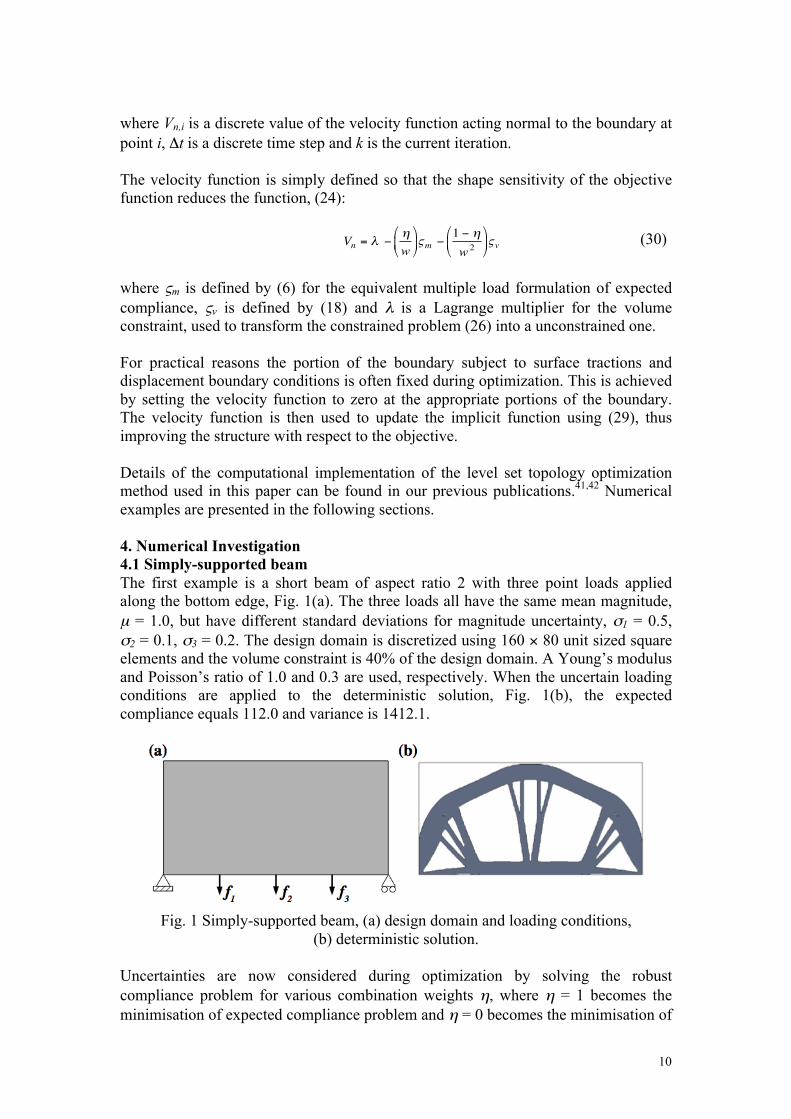
where ςm is defined by (6) for the equivalent multiple load formulation of expected compliance, ςv is defined by (18) and λ is a Lagrange multiplier for the volume constraint, used to transform the constrained problem (26) into a unconstrained one. For practical reasons the portion of the boundary subject to surface tractions and displacement boundary conditions is often fixed during optimization. This is achieved by setting the velocity function to zero at the appropriate portions of the boundary. The velocity function is then used to update the implicit function using (29), thus improving the structure with respect to the objective. Details of the computational implementation of the level set topology optimization method used in this paper can be found in our previous publications.41,42 Numerical examples are presented in the following sections. 4. Numerical Investigation 4.1 Simply-supported beam The first example is a short beam of aspect ratio 2 with three point loads applied along the bottom edge, Fig. 1(a). The three loads all have the same mean magnitude, µ = 1.0, but have different standard deviations for magnitude uncertainty, σ1 = 0.5, σ2 = 0.1, σ3 = 0.2. The design domain is discretized using 160 × 80 unit sized square elements and the volume constraint is 40% of the design domain. A Young’s modulus and Poisson’s ratio of 1.0 and 0.3 are used, respectively. When the uncertain loading conditions are applied to the deterministic solution, Fig. 1(b), the expected compliance equals 112.0 and variance is 1412.1.

Fig. 1 Simply-supported beam, (a) design domain and loading conditions,

(b) deterministic solution. Uncertainties are now considered during optimization by solving the robust compliance problem for various combination weights η, where η = 1 becomes the minimisation of expected compliance problem and η = 0 becomes the minimisation of

  11

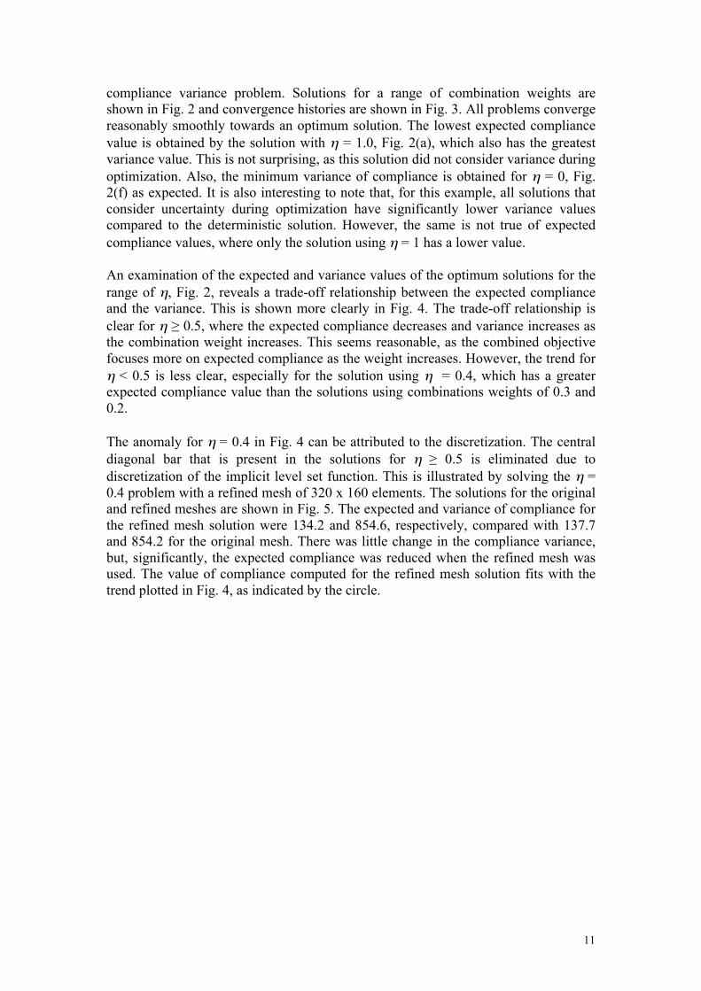
compliance variance problem. Solutions for a range of combination weights are shown in Fig. 2 and convergence histories are shown in Fig. 3. All problems converge reasonably smoothly towards an optimum solution. The lowest expected compliance value is obtained by the solution with η = 1.0, Fig. 2(a), which also has the greatest variance value. This is not surprising, as this solution did not consider variance during optimization. Also, the minimum variance of compliance is obtained for η = 0, Fig. 2(f) as expected. It is also interesting to note that, for this example, all solutions that consider uncertainty during optimization have significantly lower variance values compared to the deterministic solution. However, the same is not true of expected compliance values, where only the solution using η = 1 has a lower value. An examination of the expected and variance values of the optimum solutions for the range of η, Fig. 2, reveals a trade-off relationship between the expected compliance and the variance. This is shown more clearly in Fig. 4. The trade-off relationship is clear for η ≥ 0.5, where the expected compliance decreases and variance increases as the combination weight increases. This seems reasonable, as the combined objective focuses more on expected compliance as the weight increases. However, the trend for η < 0.5 is less clear, especially for the solution using η = 0.4, which has a greater expected compliance value than the solutions using combinations weights of 0.3 and 0.2. The anomaly for η = 0.4 in Fig. 4 can be attributed to the discretization. The central diagonal bar that is present in the solutions for η ≥ 0.5 is eliminated due to discretization of the implicit level set function. This is illustrated by solving the η = 0.4 problem with a refined mesh of 320 x 160 elements. The solutions for the original and refined meshes are shown in Fig. 5. The expected and variance of compliance for the refined mesh solution were 134.2 and 854.6, respectively, compared with 137.7 and 854.2 for the original mesh. There was little change in the compliance variance, but, significantly, the expected compliance was reduced when the refined mesh was used. The value of compliance computed for the refined mesh solution fits with the trend plotted in Fig. 4, as indicated by the circle.

  12

Fig. 2 Robust solutions for the beam example using various combination weights.

  13

Fig. 3 Convergence histories for the robust solutions of the simply-supported beam.

Fig. 4 Expectancy and variance of compliance for a range of combination weights.

  14

Fig. 5 Comparison of solution for η = 0.4, (a) Original mesh - 160 × 80, (b) Refined

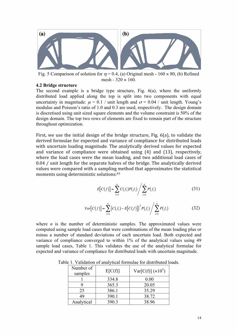
mesh - 320 × 160. 4.2 Bridge structure The second example is a bridge type structure, Fig. 6(a), where the uniformly distributed load applied along the top is split into two components with equal uncertainty in magnitude: µ = 0.1 / unit length and σ = 0.04 / unit length. Young’s modulus and Poisson’s ratio of 1.0 and 0.3 are used, respectively. The design domain is discretised using unit sized square elements and the volume constraint is 50% of the design domain. The top two rows of elements are fixed to remain part of the structure throughout optimization. First,  we  use   the   initial  design  of   the  bridge  structure,  Fig.  6(a),   to  validate   the  derived  formulae  for  expected  and  variance  of  compliance  for  distributed  loads  with  uncertain   loading  magnitude.  The  analytically  derived  values   for  expected  and   variance   of   compliance   were   obtained   using   (4)   and   (13),   respectively,  where   the   load   cases  were   the  mean   loading,   and   two  additional   load   cases  of  0.04  /  unit  length  for  the  separate  halves  of  the  bridge.  The  analytically  derived  values  were  compared  with  a  sampling  method  that  approximates  the  statistical  moments  using  deterministic  solutions:43

€

E C f( )[ ] ≈ C fi( )P fi( )i=1

n

∑ P fi( )i=1

n

∑ (31)

€

Var C f( )[ ] ≈ C fi( ) − E C f( )[ ]( )2P fi( )

i=1

n

∑ P fi( )i=1

n

∑ (32)

where n is the number of deterministic samples. The approximated values were computed using sample load cases that were combinations of the mean loading plus or minus a number of standard deviations of each uncertain load. Both expected and variance of compliance converged to within 1% of the analytical values using 49 sample load cases, Table 1. This validates the use of the analytical formulae for expected and variance of compliance for distributed loads with uncertain magnitude.

Table 1. Validation of analytical formulae for distributed loads. Number of

samples E[C(f)] Var[C(f)] (×103)

1 334.8 0.00 9 365.3 20.05 25 386.1 35.29 49 390.1 38.72

Analytical 390.3 38.96

  15

We now consider the optimization of the bridge structure. The deterministic solution is shown in Fig. 6(b). When the uncertain loading conditions are applied to the deterministic solution, the expected compliance is 1320.6 and variance is 1326.0×103. Uncertainty is now considered during optimization and the solutions for η = 1.0, 0.5, 0.0 are shown in Fig. 7(a), (b) and (c), respectively. Values for expected compliance are: 635.1, 633.7, 633.5 and values for variance are: 100.7×103, 100.3×103, 100.2×103, for η = 1.0, 0.5, 0.0, respectively. All solutions are similar to the deterministic solution, except for the addition of two lower horizontal bars. These bars support the potentially unsymmetrical loading conditions and significantly reduce the expected compliance and the variance, compared to the deterministic solution. All robust solutions are very similar in design and have compliance values within 1%. This suggests that, for this problem, the expected and variance values of compliance are mutual, such that minimizing one also minimises the other. Furthermore, the problem was solved for a range of objective weighting factors and almost identical solutions were obtained in each case. The behavior of the bridge structure is in contrast to the previous example of a simply supported beam, where there was a trade-off between the expected and variance of compliance. The two examples demonstrate that the effect of introducing compliance variance into the objective is problem dependent and it is not clear what specific features of the two examples produce this contrasting behaviour when variance is introduced. Further studies are underway to investigate and provide a more in-depth understanding for the robust optimization formulation of the expected and variance of compliance as a multi-objective problem.

Fig. 6 Optimization of the bridge structure, (a) design domain and loading conditions, (b) deterministic solution.

  16

Fig. 7 Robust optima of the bridge structure (a) expected compliance objective, (b) combined objective η = 0.5, (c) variance of compliance objective.

5 Conclusions This paper introduces an exact formulation for compliance variance under loading magnitude uncertainty for robust topology optimization. The robust objective for normally distributed uncertain loads can be computed by considering only a small number of additional load cases. This makes the robust topology optimization computational tractable (using a standard PC) and accessible by any topology optimization method. The numerical examples show substantial benefits and significant topological changes can be expected from robust optimization in comparison with the equivalent deterministic optimization. The objectives of expectancy and variance may or may not be conflicting and this depends on the specific structural design problems. Understanding of this a priori to optimization does not appear to be obvious. Acknowledgements The authors would like to thank the Numerical Analysis Group at the Rutherford Appleton Lab for their FORTRAN HSL packages. Reference 1 Kim, H., Querin ,O.M., Steven, G.P., “On development of structural optimisation

and its relevance in engineering design,” Design Studies, Vol. 23, No. 1, 2002, pp. 85-102.

2 Bendsøe, M.P., Kikuchi, N., “Generating optimal topologies in structural design using a homogenization method,” Computer Methods in Applied Mechanics and Engineering, Vol. 71, No. 2, 1988, pp. 197-224.

3 MSC Software, MSC Nastran, Santa Ana, CA, USA, 2012. 4 Dassault Systemes, Abaqus, Vélizy-Villacoublay, France, 2012. 5 COMSOL Group, COMSOL Multiphysics, Stockholme, Sweden, 2012.

  17

6 Altair Engineering Inc., Optistruct, Troy, MI, USA, 2012. 7 Schuëller, G.I., Jensen, H.A., “Computational methods in optimization considering

uncertainties – an overview,” Computer Methods in Applied Mechanics and Engineering, Vol. 198, No. 1, 2008, pp. 2-13

8 Kharmanda, G., Olhoff, N. (2001). Reliability-based Topology Optimization, Institute of Mechanical Engineering, Aalborg University, Denmark.

9 Bae, K.R., Wang, S., Choi, K.K., “Reliability-based topology optimization,” the 9th AIAA/ISSMO Symposium and Exhibit on Multidisciplinary Analysis and Optimization, Atlanta, GA, 2002.

10 Moon, H., Kim, C., Wang, S., “Reliability-based topology optimization of thermal systems considering convection heat transfer,” the 10th AIAA/ISSMO Multidisciplinary Analysis and Optimization Conference, Albany, New York, 2004.

11 Kharmanda, G., Olhoff, N., Mohamed, A., Lemaire, M., “Reliability-based topology optimization,” Structural and Multidisciplinary optimization, Vol. 26, No. 5, 2004, pp. 295–307.

12 Jung, H.S., Cho, S., “Reliability-based topology optimization of geometrically nonlinear structures with loading and material uncertainties,” Finite Element in Analysis and Design, Vol. 41, No. 3, 2004, pp. 311–331.

13 Wang, S., Moon, H., Kim, C., Kang, J., Choi, K.K., “Reliability-based topology optimization (RBTO),” IUTAM Symposium on Topological Design Optimization of Structures, Machines and Materials: Solid Mechanics and its Applications, Springer, 2006.

14 Kim, C., Wang, S.Y., Bae, K.R., Moon, H., Choi, K.K., “Reliability-based topology optimization with uncertainties,” Journal of Mechanical Science and Technology, Vol. 20, No. 4, 2006, pp. 494-504.

15 Mogami, K., Nishiwaki, S., Izui, K., Yoshimura, M., Kogiso, N., “Reliability-based structural optimization of frame structures for multiple failure criteria using topology optimization techniques,” Structural and Multidisciplinary Optimization, Vol. 32, No. 4, 2006, pp. 299-311.

16 Maute, K., Frangopol, D.M., “Reliability-based design of MEMS mechanisms by topology optimization,” Computers and Structures, Vol. 81, No. 8-11, 2003, pp. 813-824.

17 Kang, J., Luo, Y., “Non-probabilistic reliability-based topology optimization of geometrically nonlinear structures using convex models,” Computer Methods in Applied Mechanics and Engineering, Vol. 198, No. 41-44, 2009, pp. 3228-3238.

18 Choi, S., Grandhi, R.V., Canfield, R.A. (2007). Reliability-based Structural Design. London, Springer.

19 Ben-Tal, A., Nemirovski, A., “Robust truss topology design via semidefinite programming,” SIAM Journal on Optimization, Vol. 7, No. 4, 1997 pp. 991-1016.

20 Alvarez, F., Carrasco, M., “Minimization of the expected compliance as an alternative approach to multiload truss optimization,” Structural and Multidisciplinary optimization, Vol. 29, No. 6, 2005, pp. 470–476.

21 Christiansen, S., Patriksson, M., Wynter, L. “Stochastic bilevel programming in structural optimization,” Structural and Multidisciplinary Optimization, Vol. 21, No. 5, 2001, pp. 361–371.

22 Guest J.K., Igusa, T., “Structural optimization under uncertain loads and nodal locations,” Computer Methods in Applied Mechanics and Engineering, Vol. 198, No. 1, 2008, pp. 116-124.

23 Ben-Haim, Y., Elishakoff, I. (1990). Convex Models of Uncertainty in Applied

  18

Mechanics. Amsterdam: Elsevier. 24 Conti, S., Held, H., Pach, M., Pumpf, M., Schultz, R., “Optimization under

uncertainty – A stochastic programming perspective,” SIAM Journal on Optimization, Vol. 19, No. 4, 2009, pp. 1610-1632.

25 Kanno, Y., Takewaki, I., “Semidefinite programming for uncertain linear equations in static analysis of structures,” Computer Methods in Applied Mechanics and Engineering, Vol. 198, No. 1, 2008, pp. 102-115.

26 Kocvara, M., Zowe, A., Nemirovski, A, “Cascading - an approach to robust material optimization”, Computers and Structures, Vol. 76, No. 1-3, 2000, pp. 431-442.

27 Cherkaev, E., Cherkaev, A., “Minimax optimization problem of structural design,” Computers and Structures, Vol. 86, No. 13-14, 2008, pp. 1426-1435.

28 Takezawa, A, Nii, S., Kitamura, M., Kogiso, N., “Topology optimization for worst load conditions based on the eigenvalue analysis of an aggregated linear system,” Computer Methods in Applied Mechanics and Engineering, Vol. 200, No. 25-28, 2011, pp. 2268-2281.

29 Dunning, P. D., Kim, H. A., Mullineux G, “Introducing Loading Uncertainty in Topology Optimization,” AIAA Journal, Vol. 49, No. 4, 2011, pp. 760-768.

30 Asadpoure , A., Tootkaboni, M., Guest, J.K., “Robust topology optimization of structures with uncertainties in stiffness – Application to truss structures,” Computers and Structures, Vol. 89, 2011, pp.1131–1141.

31 Tootkaboni, M., Asadpoure , A., Guest, J.K., “Topology optimization of continuum structures under uncertainty – A Polynomial Chaos approach,” Computer Methods in Applied Mechanics and Engineering, Vol. 201–204, 2012, pp. 263–275.

32 Kogiso, N., Ahn, W., Nishiwaki, S., Izui, K., Yoshimura, M. “Robust topology optimization for compliant mechanisms considering uncertainty of applied loads. Journal of Advanced Mechanical Design Systems and Manufacturing, Vol. 2, No.1, 2008, pp. 96-107.

33 Chen, S., Chen, W., Lee, S., “Level set based robust shape and topology optimization under random field uncertainties,” Structural and Multidisciplinary Optimization, Vol. 41, No. 4, 2010, pp. 507-24.

34 Seepersad C. C., Alien, J. K., Mcdowell, D. L., Mistree, F. “Robust design of cellular materials with topological and dimensional imperfections,” Transactions of the American Society of Mechanical Engineers, Journal of Mechanical Design, Vol. 128, No. 6, 2006, pp. 1285-1297.

35 Carrasco, M., Ivorra, B., Ramos, A. M., “A variance-expected compliance model for structural optimization”, Journal of Optimization Theory and Applications, Vol. 152, No. 1, 2012, pp. 136-151.

36 Allaire, G., Jouve, F., “A level-set method for vibration and multiple loads structural optimization.” Computer Methods In Applied Mechanics and Engineering, Vol. 194, 2005, pp. 3269-3290.

37 Allaire, G., Jouve, F., Toader, A.M., “Structural optimization using sensitivity analysis and a level-set method,” Journal of Computational Physics, Vol. 194, No. 1, 2004, pp. 363-393.

38 Su, J., Renaud, J. E., “Automatic differentiation in robust optimization,” AIAA Journal, Vol. 35, No. 6, 1997, pp. 1072-1079.

39 Wang, M.Y., Wang, X., Guo, D., “A level set method for structural topology optimization,” Computer Methods In Applied Mechanics and Engineering, Vol 192, No. 1-2, 2003, pp. 227-246.

  19

40 Sethian, J., Wiegmann, A. “Structural boundary design via level-set and immersed interface methods,” Journal of Computational Physics, Vol. 163, 2000, pp. 489-528.

41 Dunning, P.D., Kim, H.A., “A new hole insertion method for level set based structural topology optimization”, International Journal for Numerical Methods in Engineering, Vol. 93, 2013, pp. 118–134.

42 Dunning, P.D., Kim, H.A., Mullineux, G., “Investigation and improvement of sensitivity computation using the area-fraction weighted fixed grid FEM and structural optimization,” Finite Elements in Analysis and Design, Vol. 47, 2011, pp. 933-941.

43 Park, G-J., Lee, T-H., Lee, K.H., Hwang, K-H., “Robust design: An overview”, AIAA Journal, Vol. 44, No. 1, 2006, pp. 181-191.