A new fully three-dimensional numerical model for ice dynamics

Alberto DEPONTI, Vincenzo PENNATI, Lucia DE BIASE, Valter MAGGI, Fabio BERTADipartimento di Scienze dell’Ambiente e del Territorio, University of Milano–Bicocca, I-20126 Milan, Italy

E-mail: alberto.deponti@unimib.it

ABSTRACT. The problem of describing ice dynamics has been faced by many researchers; in this paper afully three-dimensional model for ice dynamics is presented and tested. Using an approach followed byother researchers, ice is considered a non-linear incompressible viscous fluid so that a fluid-dynamicapproach can be used. The model is based on the full three-dimensional Stokes equations for thedescription of pressure and velocity fields, on the Saint-Venant equation for the description of the free-surface time evolution and on a constitutive law derived from Glen’s law for the description of iceviscosity. The model computes the complete pressure field by considering both the hydrostatic andhydrodynamic pressure components; it is time-evolutive and uses high-order numerical approximationfor equations and boundary conditions. Moreover it can deal with both constant and variable viscosity.Three theoretical tests and two applications to Priestley Glacier, Antarctica, are presented in order toevaluate the performance of the model and to investigate important phenomena of ice dynamics such asthe influence of viscosity on pressure and velocity fields, basal sliding and flow over perturbed bedrocks.All these applications demonstrate the importance of treating the complete pressure and stress fields.

LIST OF SYMBOLS

a ¼ as � að�bÞNet accumulation/ablation rate

að�bÞ Basal melting/refreezing rate

as Surface accumulation/ablation rateB0 Viscosity parameter�b Bedrock depthC Basal sliding coefficient

g ¼ ½gx , gy , gz �TGravity acceleration vector

n Glen’s law exponent

n ¼ ½nx , ny , nz �TOutward normal unitary vector

p Kinematic pressureQ Creep activation energyq Time indexR Perfect gas constantS ¼ sðx, y, tÞ � z

Free-surface functions Free-surface elevations0 Undisturbed reference levelT Temperaturet Time

u ¼ ½u, v, w�TVelocity vector

uð�bÞ ¼ ½uð�bÞ, vð�bÞ, wð�bÞ�TBasal velocity vector

x ¼ ½x, y, z�TSpace coordinates

� Difference of a quantity between two successiveiterates

�t Time-step�x, �y, �z

Control volume dimensions

_"0 Small number to prevent singularities in Glen’s law� Non–hydrostatic part of p� Density of ice

�ð�bÞ ¼ �� ðnT � � � nÞI� � � nBasal stress vector

� Stress tensor

�e ¼ 12 tr ð�þ �pIÞ2h in o1

2

Effective stress�ij Stress tensor components

� Kinematic viscosity� ¼ ½�, �, ��

Space coordinates of a local reference systemr Gradient operatorr� Divergence operator

1. INTRODUCTIONOne of the main challenges in glaciological sciences isunderstanding glacier dynamics, in terms of mass andthermal flows, basal processes and responses to climatechange. Many authors have faced the problem of describingice dynamics through numerical modelling. Most of thelarge-scale ice-sheet models are based on the shallow-iceapproximation (SIA) which, by assuming a small aspectratio between vertical and horizontal dimensions of thedomain, neglects part of the stresses and considers thepressure hydrostatic. After the original work of Mahaffy(1976), a number of models have been proposed andapplied to studying ice-sheet dynamics (Jenssen, 1977;Huybrechts 1990; Greve,1997; Ritz and others, 1997;Calov and others, 1998). SIA models have also been usedto study the motion field in valley glaciers (Hubbard andothers, 1998; Le Meur and Vincent, 2003). The hypothesisof a small aspect ratio, on which the SIA relies, may fail onmedium- and small-scale applications. A way to improvethese models is represented by the higher-order models in

Journal of Glaciology, Vol. 52, No. 178, 2006 365

which second-order stresses are considered (Gudmunds-son, 1997a, b; Colinge and Blatter, 1998; Pattyn, 2002). Atwo-dimensional method, in which the equations areintegrated line by line over the ice depth in order tocompute the basal conditions, is proposed by Van derVeen (1989) and Van der Veen and Whillans (1989). Atwo-dimensional ice-sheet model in which a projectionmethod is used for the time-advancing scheme andclassical second-order finite-difference formulae are usedfor the space discretization is presented by Mangeney andothers (1997). Commercial finite-element codes have alsobeen used for modelling ice dynamics (Gudmundsson,1999; Luthi and Funk, 2000, 2001). Some finite-differencetime-advancing schemes are presented and compared inGreve and Calov (2002). A recent work (Martın andothers, 2004) includes a complete treatment of thepressure field.

The target of the present work is the implementation of ageneral three-dimensional method capable of working onlarge- and small-scale applications. For this reason a fluid-dynamic approach has been considered and a methodcapable of modelling the full stress and pressure fields ispresented. The full pressure field is computed by splitting thepressure into hydrostatic and hydrodynamic components(Casulli, 1999; Casulli and Zanolli, 2002). It should benoticed that no stress component is neglected in theproposed method. The use of fully three-dimensional equa-tions requires the imposition of boundary conditions on allthe domain boundaries, not only on surface and bedrock asusually done in SIA and higher-order models thanks to thesmall-aspect-ratio hypothesis. The model is based on theStokes equations and the Saint-Venant equation which arediscretized in space by means of the finite-volume methodin order to guarantee both local and global mass andmomentum conservation. High-order approximations areused for the discretization of equations and boundaryconditions. The equations are discretized in time by amodified projection method that can take the free-surfacetime evolution into account.

The paper is organized as follows: In section 2 thegoverning equations are presented. In section 3 the spaceand time discretization of these equations is presentedtogether with the description of the boundary conditions. Forclarity, in this section only the time semi-discretization of thefield equations is presented; the space- and time-discretizedequations and the formulae for the approximation of thederivatives are given in Appendices A and B, respectively. Insection 4 three theoretical applications are presented and insection 5 the model is applied to the real case of PriestleyGlacier, Antarctica. Finally in section 6 some conclusionsare drawn.

2. GOVERNING EQUATIONSFollowing the approach proposed by Nye (1952) andcommonly accepted and used in glaciological studies, iceis a non-Newtonian viscous fluid, governed by the Navier–Stokes equations. If a meso- or large-scale model isinvestigated, then convective terms are negligible since theyact on a much smaller space- and timescale (Colinge andBlatter, 1998); however, when small-scale phenomena are tobe investigated (frontal movements, crevasse opening, etc.),convective terms might be retained. In what follows, theunsteady Stokes equations for an incompressible fluid will

be considered; the equations written in conservation formare:

@u@t

�r � � ruð Þ þ ruð ÞTh in o

¼ �rp þ g, ð1Þr � u ¼ 0, ð2Þ

where u ¼ ½u, v,w�T is the three-dimensional velocityvector, t is the time, r� is the divergence operator, r isthe gradient operator, � is the kinematic viscosity,p ¼ trð�Þ=3� is the kinematic pressure and g is the gravityacceleration vector. The strain-rate tensor is represented by

ruð Þ þ ruð ÞTh i.

2:

For temperate ice masses, when large- or mesoscaleapplications are investigated, the term @u=@t can beneglected, the only transient development being surfaceevolution. In these cases the time derivative can be used tonumerically solve Equations (1) and (2) until a steady state isreached (Mangeney and others, 1997).

The momentum equation (1) can be written as

@u@t

�r � � ruð Þ½ � ¼ �rp þ gþ r� � ruð ÞTh i

, ð3Þ

so that the momentum equation for the single velocitycomponents can be solved separately. The term r � � ruð Þ½ �will be called the ‘diffusive term’.

Ice viscosity is described by the following relation derivedfrom Glen’s law:

� ¼ 12�

B0 expQnRT

� �� 1

2@u@x

� �2

þ @v@y

� �2

þ @w@z

� �2" #(

þ14

@u@y

þ @v@x

� �2

þ @u@z

þ @w@x

� �2

þ @v@z

þ @w@y

� �2" #)1

2

þ _"0

!1�nn

, ð4Þ

where B0 is the viscosity parameter, Q is the activationenergy for creep, R is the perfect gas constant, T is thetemperature, n is the exponent in Glen’s law and _"0 is asmall number (e.g. 10–30 a–1) used to avoid singular be-haviour where the stress vanishes.

The surface of an ice mass is a stress-free surface that canevolve in time. The surface evolution can be caused bychanges in the inner motion field as well as by changes inthe accumulation/ablation rate. Denoting the surface eleva-tion above an undisturbed reference level by s, the kinematicboundary condition for the free surface is

@s@t

þ u@s@x

þ v@s@y

�w ¼ as, ð5Þ

where as is the accumulation/ablation rate at the surfacemultiplied by the modulus of the gradient of the free surfacefunction ðjrSj ¼ j @s=@x, @s=@y, �1ð ÞTjÞ. Denoting thedepth of the bedrock with respect to the undisturbedreference level by �b, the kinematic boundary conditionfor the ice/bedrock interface is

u@ð�bÞ@x

þ v@ð�bÞ@y

�w ¼ að�bÞ, ð6Þ

where að�bÞ is the basal melting/refreezing rate multiplied bythe modulus of the bedrock gradient.

Deponti and others: A new fully 3-D numerical model for ice dynamics366

Integration of the incompressibility equation (2) from thebedrock to the surface and substitution of Equations (5)and (6) lead to the Saint-Venant equation:

@s@t

þ @

@x

Z s

ð�bÞu dz þ @

@y

Z s

ð�bÞv dz ¼ a, ð7Þ

where a ¼ as � að�bÞ. This equation describes the freesurface evolution in time as a function of the unit-dischargesand incorporates the physical law of mass conservation.

3. NUMERICS3.1. Space discretizationA solution in closed form for the unsteady three-dimensionalStokes problem is not known, even in simple cases; thus anapproximated solution has to be computed by numericalmethods. Conservation of mass and momentum is crucial forthe stability and the accuracy of the solution, especially inthe presence of a moving boundary such as the free surface(Deponti and others, 2004). The finite-volume method isused for the discretization of the field equations since itguarantees both local and global conservation of mass andmomentum.

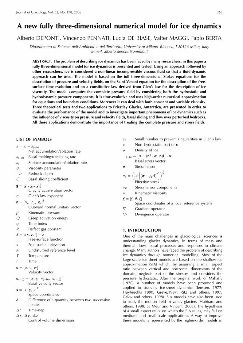
An undisturbed reference level s0 coincident with thelinear least-squares approximation of the physical surface isconsidered. In the reference system used, the x-y plane lieson s0, the x axis is oriented along the mean flow directionand points downhill, the z axis points upward and the y axisis consequently determined. The domain is partitioned bymeans of cell-centred control volumes in the shape ofrectangular prisms (Fig. 1); each control volume face isorthogonal to one coordinate axis, and the union of all thecontrol volumes determines the computational domain. Thedimensions of each control volume are �x, �y and �z. Thevolume horizontal dimensions are chosen on the basis of apriori knowledge of the domain peculiarities and are fixedthroughout computation. The volume height is also fixedwith the same criterion for the volumes far from the freesurface, but, due to its evolution, the height of thoseincluding the free surface can change in time and it may benecessary to add or suppress some volumes; this is why thedimension �z will be time-indexed from now on. Controlvolumes filled with ice are called active.

The field equations are integrated on each controlvolume; by the Green–Gauss theorem this leads to com-puting the surface integral of the flux of the diffusive terms(diffusive fluxes). These are calculated by summing thecontributions of each control volume face, i.e. using theproduct of the representative value of the diffusive term andof the face area (integral mean value theorem). Hence,diffusive fluxes are to be approximated on each controlvolume face; this is done by a four-point centred differencingscheme (see Appendix B for details). The scheme is generalenough to allow for non-uniform spacing between adjacentpoints and is third-order accurate. The volume integrals areapproximated using the integral mean value theorem.

3.2. Time-advancing schemeA method for time integration of Stokes equations withoutparticular assumptions on the pressure field is the projectionmethod (a particular type of fractional step method) in whichthe equations are integrated in two or more steps. Thismethod is widely used in fluid dynamics, and many

formulations have been proposed in the literature (e.g.Gresho, 1991; Guermond and Quartapelle, 1998; Armfieldand Street, 2002).

The projection method alone cannot describe the freesurface evolution, and direct calculation of the kinematicboundary condition at the surface (Equation (5)) or of theSaint-Venant equation (7) may lead to physical inconsis-tency and to numerical instability. Indeed, the kinematicboundary condition and the Saint-Venant equation are to becomputed on the basis of a velocity field consistent with thenew surface elevation in spite of its being unknown; thiscould become important in the presence of accumulation/ablation or in the presence of varying dynamic boundaryconditions at the surface. For these reasons, a modifiedprojection method in which the Saint-Venant equation iskept in order to calculate the free-surface evolution isproposed in this work.

As mentioned in the Introduction, the pressure in an icemass is not always hydrostatic; in particular, in the presenceof bedrock perturbations or of changes in the basal slidingconditions a hydrodynamic pressure occurs. This phenom-enon is also called the ‘bridging effect’ (Van der Veen andWhillans, 1989; Blatter and others, 1998). The totalkinematic pressure, p, is divided into the hydrostatic part,jgjðs � zÞ, and the hydrodynamic part, �,

p ¼ jgjðs � zÞ þ �: ð8ÞIn the first step, provisional velocities ~uqþ1 are calculated byconsidering the contribution of the hydrostatic pressure atthe preceding time-step, q, and neglecting the contributionof the hydrodynamic pressure:

~uqþ1 �uq

�t�r � �qr ~uqþ1� �

¼ �jgjrSq þ gþ r�q � ruqð ÞTh i

, ð9Þ

where rSq ¼ @sq=@x, @sq=@y, �1ð ÞT is the gradient of thefree surface function and the superscripts represent the timeindices. The physical boundary conditions for the threevelocity components are imposed on all boundaries. In thefirst step the incompressibility equation is not considered sothat the provisional velocity field is, in general, non-divergence-free.

The target of the second step of the projection method isthe formulation of a second-order equation for the totalpressure or for a part of it, in which the mass conservation

Fig. 1. Sketch of a three-dimensional control volume.

Deponti and others: A new fully 3-D numerical model for ice dynamics 367

principle (expressed by the null-divergence constraint) isaccounted for. In our formulation the second-order equationfor the hydrodynamic pressure, �, is obtained by applyingthe divergence operator to the momentum equation writtenin the form

uqþ1 � ~uqþ1

�t¼ �r�qþ1 ð10Þ

and considering the null-divergence constraint

r � r�qþ1 ¼ 1�t

r � ~uqþ1 : ð11Þ

This equation holds for the control volumes not connectedto the surface. In the presence of a moving surface, the massconservation and the compatibility between the velocityfield and the surface geometry are guaranteed by acombination of the incompressibility equation (2) and theSaint-Venant equation (7). Hence, the discretized form of theequation for � at the surface control volumes is obtained bycombining the discretized form of Equations (2) and (7)(Equation (A13) in Appendix A). The second-order discre-tized equation for � is thus given by the conjunction of thediscretized form of Equation (11) (Equation (A8) inAppendix A) and the discretized equation at the surface(Equation (A13) in Appendix A). Homogeneous Neumannboundary conditions are imposed at all boundaries.

Once the hydrodynamic pressure is calculated, the finalvelocity field is computed by Equation (10); assuming thepressure to be hydrostatic only in the surface controlvolumes, the final free-surface elevation is computed by

sqþ1 ¼ sq þ �qþ1

jgj : ð12Þ

The final velocity field is divergence-free since the massconservation has been imposed in the second step; more-over the free-surface elevation is consistent with the innervelocity field since the Saint-Venant equation has beenconsidered.

3.3. Boundary conditionsAs said above, physical boundary conditions for the threecomponents of the velocity field are applied at all bound-aries in the first step, while homogeneous Neumannboundary conditions are imposed in the second step for

the hydrodynamic pressure at all boundaries. Let us focus onthe boundary conditions for the velocity field. At the openboundaries (inflow and outflow sections), homogeneousNeumann boundary conditions are applied. At the surfacethe stress-free condition applies. At lateral solid walls and atthe bedrock the impenetrability condition holds for thenormal velocity component, while a sliding condition isrequired for the tangential and binormal velocity com-ponents. The relation between basal stress and slidingvelocity is expressed by

uð�bÞ � C�2ð�bÞ�ð�bÞ ¼ 0, ð13Þ

where uð�bÞ is the basal velocity vector, C is a slidingparameter and

�ð�bÞ ¼ ½�� ðnT � � � nÞI� � n ð14Þis the basal stress vector, I being the identity matrix. Thethree-dimensional sliding relation (13) automatically satis-fies the impenetrability condition expressed by Equation (6)where að�bÞ ¼ 0 (Hutter, 1983). If C ¼ 0 the relationtranslates into the no-slip condition, i.e. homogeneousDirichlet; if C ! 1 the condition translates into the perfectslip condition, i.e. homogeneous Neumann. In all othercases the condition is a Robin boundary condition andallows the computation of stress and sliding velocity at thesame time.

Numerical boundary conditions are approximated bymeans of high-order (second and third) generalized finite-difference formulae (presented in Appendix B); this yields agood approximation of the boundary conditions and allowsfor non-uniform volume dimensions. In particular, thecontrol volumes can be smaller where a better accuracy ofthe solution is required.

4. THEORETICAL APPLICATIONSThe applications presented in this section aim to evaluatethe method performance and to investigate importantaspects in ice dynamics such as the influence of viscosityon velocity and pressure fields, basal sliding and flow overundulating bedrocks. For these targets it is useful to considertheoretical tests in which the aspect being investigated canbe emphasized; hence two-dimensional tests are consid-ered. Even though the problems are two-dimensional, theyare modelled in a complete three-dimensional setting wherehomogeneous Neumann conditions are imposed in thetransverse direction (y direction). Results will be presentedin vertical sections (x-z planes).

Steady-state solutions are calculated starting from anundisturbed situation; the time discretization is chosen onthe basis of the desired accuracy and of the stabilityconditions imposed by the method. The iterations arestopped when the difference, �, between two successiveiterates is smaller than a fixed tolerance. This difference iscomputed on the whole domain by

� ¼

ffiffiffiffiffiffiffiffiffiffiffiffiffiffiffiffiffiffiffiffiffiffiffiffiffiffiffiffiffiffiffiffiffiffiffiffiffiffiffiffiffiffiffiffiffiffiffiffiPjP

i ðuqþ1i � uq

i Þ2h i

j

rffiffiffiffiffiffiffiffiffiffiffiffiffiffiffiffiffiffiffiffiffiffiffiffiffiffiffiffiffiffiffiffiffiP

jP

i ðuqi Þ2

h ij

r , ð15Þ

where the i index describes the three velocity componentsand the j index extends to all control volumes.

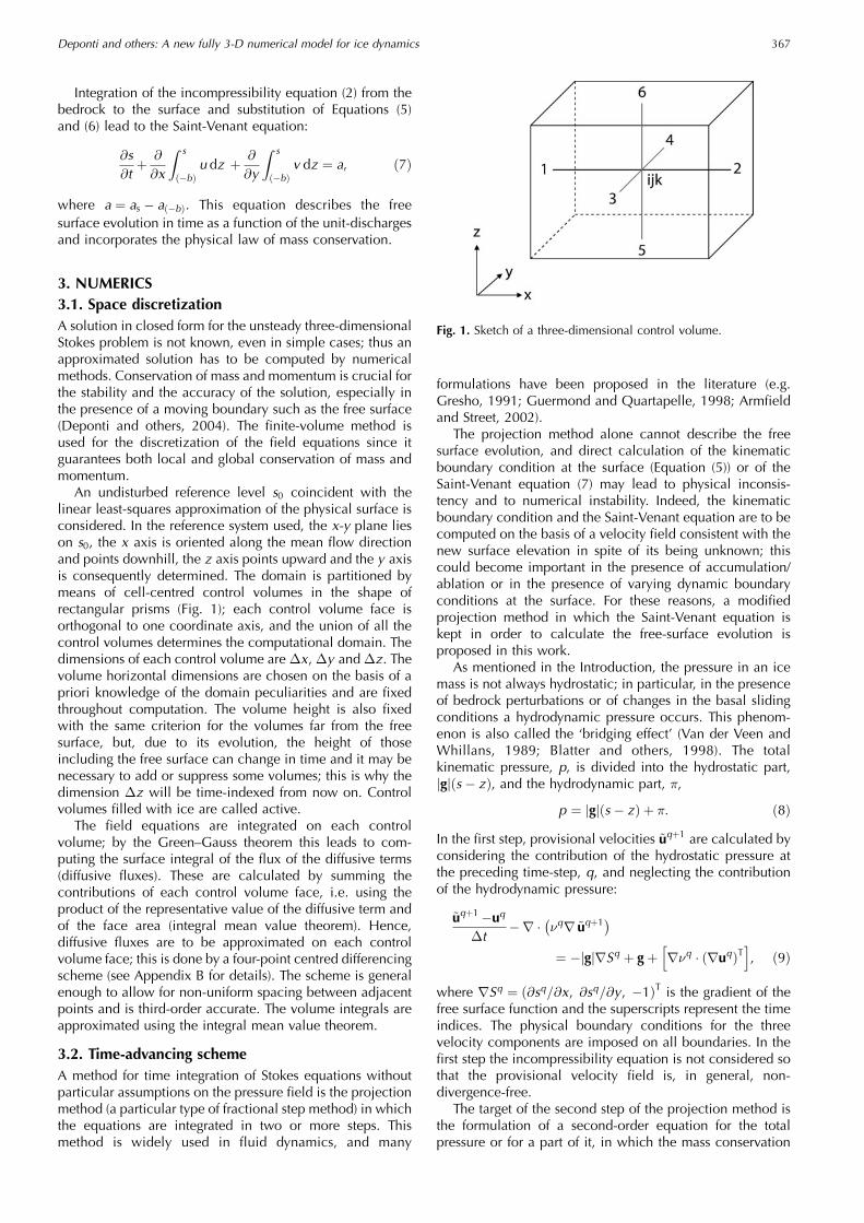
Fig. 2. Vertical profile of the longitudinal velocity for threekinematic viscosities: � ¼ 1011m2 s–1 (solid line), � ¼ 1012m2 s–1

(dashed line), � ¼ 1013m2 s–1 (dotted line).

Deponti and others: A new fully 3-D numerical model for ice dynamics368

4.1. Uniformly inclined plane

In the first application a section of an infinite slab isconsidered. Surface and bedrock are flat, parallel andinclined at a small angle (58). The expected solution is theso-called ‘laminar flow regime’ (Nye, 1952; Paterson, 1994)in which the vertical and transverse velocity components arenull and the free surface remains undisturbed. The domain ispartitioned into 1575 control volumes (21 rows in thex direction, 25 in the z direction and 3 in the y direction),of which 1512 are active; the time-step, Dt, is 0.5 years.Iterations are stopped for � � 10�4. Different sliding par-ameters, ranging from the no-slip condition to the perfect slip

condition, are tested. In all cases the velocity field agreeswiththe expected solution, the free surface remains undisturbedand the velocity divergence is null everywhere. Differentconstant values of the kinematic viscosity are tested.

In Figure 2 the vertical profile of the horizontal velocitycomponent for the no-slip case is presented for threedifferent kinematic viscosities: � ¼ 1011, 1012, 1013m2 s–1.The number of iterations performed to reach the steady statewere 508, 134 and 26 for the three viscosity values,respectively. The model sensitivity to viscosity changes canbe appreciated. It can be seen that the lower the viscosity,the higher the surface velocity; since no-sliding conditionsapply, for lower viscosity vertical deformations are larger.

Fig. 3. (a) Velocity field, (b) free surface and (c) hydrodynamicpressure field of the flow in the presence of variations in basalslipperiness. The components of the gravity acceleration vector inthe considered reference system are gx ¼ 0:855, gy ¼ 0:000,gz ¼ �9:773 (see section 3.1). Negative and positive hydrodynamicpressures arise in the vicinity of slipperiness variations; thesekinematic pressures are related to vertical velocities and free-surface perturbations. Note the different scales of horizontal andvertical axes.

Fig. 4. (a) Velocity field, (b) free surface and (c) hydrodynamicpressure field of the flow over an undulating bedrock. Thecomponents of the gravity acceleration vector in the consideredreference system are gx ¼ 0:855, gy ¼ 0:000, gz ¼ �9:773 (seesection 3.1). The velocities in the vicinity of the bedrock follow thebasal undulations; positive hydrodynamic pressure upstream andnegative hydrodynamic pressure downstream of undulations can beappreciated. The free surface presents perturbations similar tobedrock undulations.

Deponti and others: A new fully 3-D numerical model for ice dynamics 369

4.2. Variations in basal slipperinessIn the second application the influence of variations in basalslipperiness on pressure and velocity fields and, conse-quently, on the free-surface geometry are investigated. Theproposed test is similar to the one presented in Blatter andothers (1998) and Colinge and Blatter (1998): an infinite slabis considered but in this case the sliding parameter C varieslocally. In particular, an 8 km long and 1 km deep domain isconsidered; the bedrock is inclined at 58 with respect to thehorizontal direction. Perfect slip conditions are prescribed ina 1 km long central portion of the domain while no-slipconditions are prescribed elsewhere. The domain is parti-tioned into 3024 active control volumes (72 rows in thex direction, 14 in the z direction and 3 in the y direction);the time-step, Dt, is 0.5 years. Iterations are stopped for� � 10�4; a total of 470 iterations were performed to reachsteady state.

In Figure 3 the results of the simulation with a constantkinematic viscosity � ¼ 1012 m2 s–1 are presented. InFigure 3a the velocity field is shown: it can be seen how,in the vicinity of the slipperiness variations, verticalvelocities increase. These vertical velocities produce aperturbation of the free surface that can be appreciated inFigure 3b. The apparent positive local slope of the freesurface (in this and in subsequent figures) is due to theinclined reference system adopted and to the differingvertical and horizontal scales. Finally, in Figure 3c thehydrodynamic pressure field is presented: it can be seen thatin the presence of slipperiness variations the pressure field isnot purely hydrostatic. Indeed, where the sliding conditions

change from no-slip to perfect slip, a longitudinal extension(accompanied by negative hydrodynamic pressure) occurswhile a longitudinal compression (accompanied by positivehydrodynamic pressure) occurs when the sliding conditionschange from perfect slip to no-slip. As mentioned insection 3.2, this phenomenon is called the bridging effect.Even if the hydrodynamic pressure is about two orders ofmagnitude smaller than the total pressure, it is related tovertical velocities and surface perturbations. This testconfirms the importance of a complete treatment of pressureand stress fields in the solution of the full Stokes problem.

4.3. Undulating bedrockIn the third application the influence of bedrock undulationson pressure and velocity fields and, consequently, on thefree-surface geometry are investigated. Similar investigationshave been performed by Gudmundsson (1997a, b, 2003),Schoof (2002) and Hindmarsh (2004). In our simulation a4 km long domain is considered. The mean domainthickness is 1 km, while the mean bedrock inclinationis 58. The amplitude of the bedrock undulations is 100m;viscous-slip conditions are imposed on the whole bedrockwith sliding parameter C ¼ 1019m s–1 Pa–2. In the firstsimulation a constant kinematic viscosity, � ¼ 1012m2 s–1,is considered. Iterations are stopped for � � 10�4; a total of286 iterations were performed to reach steady state. Thedomain is partitioned into 2160 control volumes (36 rows inthe x direction, 20 in the z direction and 3 in they direction), of which 1515 are active; the time-step, Dt, is0.5 years. In Figure 4a the velocity field is presented: it can

Fig. 5. (a) Velocity field, (b) free surface, (c) hydrodynamic pressure field and (d) viscosity distribution of the flow over an undulating bedrockwith variable viscosity. The presence of positive and negative hydrodynamic pressures and of vertical velocities following the bedrock can beappreciated. Minimum viscosity (�1011m2 s–1) is found near the bedrock, while maximum viscosity (�1013m2 s–1) is found at the surface.Because of the higher velocities, the free surface is more inclined than with constant viscosity.

Deponti and others: A new fully 3-D numerical model for ice dynamics370

be seen that the velocities in the vicinity of the bedrockfollow the basal undulations. The vertical velocity com-ponent influences the free-surface geometry that, as shownin Figure 4b, exhibits perturbations similar to thosepresented by the bedrock but with smaller amplitude. InFigure 4c the kinematic hydrodynamic pressure field ispresented; it can be seen that longitudinal compressions(accompanied by positive pressures) occur upstream of thebedrock undulations while longitudinal extensions (accom-panied by negative pressures) occur downstream; thishydrodynamic pressure is related to vertical velocitieswhich, in turn, are responsible for surface perturbations.

In the second simulation the same domain and thesame partition are considered but viscosity is computedby Equation (4); the value of B ¼ B0 exp ðQ=nRT Þ=2 is

1.3�105 s1/3 kPa. The term r�q � ruqð ÞTh i

on the righthand

side of Equation (9) is neglected, as is usual in fluiddynamics; for variable viscosity this implies neglecting partof the stress field. Results are presented in Figure 5. Iterationsare stopped for � � 10�3; 768 iterations were performed toreach steady state. It can be seen that the results aresignificantly different from those with constant viscosity. Inparticular, from Figure 5a, it can be seen that the velocityfield is higher since the viscosity is smaller near the bedrockdue to high strain rates. Minimum viscosity (�1011m2 s–1) isindeed found near the bedrock; maximum viscosity(�1013m2 s–1) is found near the surface. In Figure 5d it isworth noting that near-surface viscosity is not constant dueto deformations of different amplitudes. Since the velocityfield is higher than in the preceding simulation, the free-surface geometry tends to be more inclined than the meanbedrock due to the high mass flow at the inflow boundary(Fig. 5b). Moreover, due to the combined effect of a highervelocity field and a higher viscosity at the surface, theperturbations at the free surface are smaller. In thisapplication more than one volume layer is affected by thefree-surface evolution; the shortwave perturbations near theinflow are produced by the inclusion of new controlvolumes and by the particular discretization of the surface;they have no physical meaning, nor are they numericalinstabilities. The higher velocity produces higher absolute

values of the kinematic hydrodynamic pressure in thevicinity of bedrock undulations (Fig. 5c). In Figure 6 thevertical profiles of the longitudinal velocity at the domaincentre (x ¼ 2.056 km, y ¼ 0.075 km) in conditions of con-stant (solid line) and variable (dashed line) viscosity arecompared. It can be seen that for variable viscosity theprofile shows the typical shape expected for non-linearfluids; ice is indeed stiffer near the surface and softer nearthe bedrock; for this reason, vertical variations in thelongitudinal velocity are concentrated near the bedrockwhile they are comparatively small near the surface.

5. A REAL CASE APPLICATION: PRIESTLEY GLACIERPriestley Glacier is an Antarctic glacier that starts fromVictoria Land Plateau and flows into Nansen Ice Sheet; it isabout 96 km long. It flows into a narrow valley which isabout 7 km wide, and its flow is almost unidirectional. Inthis application we consider a portion of Priestley Glacier13 km long and 6 km wide, around a reference point P withcoordinates 74819’ S, 162891’ E (Baroni, 1996). Since thedomain is narrower than the valley, some ice/ice interfacesoccur on lateral walls. Surface topography is calculatedusing the RAMP (RADARSAT-1 Antarctic Mapping Project)database, while bedrock topography is calculated by inte-grating BEDMAP data and radio-echo soundings (personalcommunication from I. Tabacco, 2004).

Fig. 6. Comparison between the vertical profiles of the longitudinalvelocity of the simulation with constant viscosity (solid line) andvariable viscosity (dashed line) in the centre of the domain withundulating bedrock. The sliding velocity is 1.3ma–1 for theconstant viscosity case and 0.9ma–1 for the variable viscosity case.

Fig. 7. (a) Velocity field in the central longitudinal section(y ¼ 3000m) and (b) free surface of case A of the application toPriestley Glacier. The components of the gravity acceleration vectorin the considered reference system are gx ¼ 0:170, gy ¼ 0:012,gz ¼ �9:809 (see section 3.1). The velocities are strongly affectedby the bedrock geometry, and the surface undulations are of thesame amplitude as the measured ones. Shortwave undulations ofthe surface are due to the coarse discretization.

Deponti and others: A new fully 3-D numerical model for ice dynamics 371

The study is performed with two different spacediscretizations in order to evaluate the model performanceand the computational effort; calculated velocities arecompared to the measured surface velocity at P. It shouldbe noted that the bedrock geometry may change whenusing different discretizations; indeed the use of smallercontrol volumes allows for a better representation of thebedrock.

In the first case (case A) the domain is partitioned into3528 control volumes (21 rows in the x direction, 12 in they direction and 14 in the z direction), of which 2301 areactive. In the second case (case B) the domain is partitionedinto 13 860 control volumes (66 rows in the x direction, 15in the y direction and 14 in the z direction), of which 9202are active. In both cases the time-step, Dt, is 0.1 years. Thesolution is calculated starting from an unperturbed situationwith constant viscosity and no-slip conditions on all solid

walls; after the velocity field is developed, the viscosity iscalculated by Equation (4), with sliding coefficients chosenin order to calculate the steady-state solution. The highsurface velocities allow the hypothesis of basal slidingconditions; on this basis an average temperature of –108C isused so that the value of B is 1.3�105 s1/3 kPa. The slidingparameters on all control volume faces lying on the bedrockare C ¼ 6� 1018m s–1 Pa–2 and C ¼ 2�1018m s–1 Pa–2 forcases A and B, respectively. On lateral walls where ice/iceinterface occurs C ! 1 is used in both cases. Timeiterations are 10 000 for case A and 12810 for case B; inboth cases the final � is less than 10�4.

Unlike the preceding theoretical tests, in this applicationnone of the righthand-side terms are neglected, � iscomputed by Equation (23) on all control volumes andhomogeneous Dirichlet boundary conditions are imposed atinflow and outflow for v, w and �.

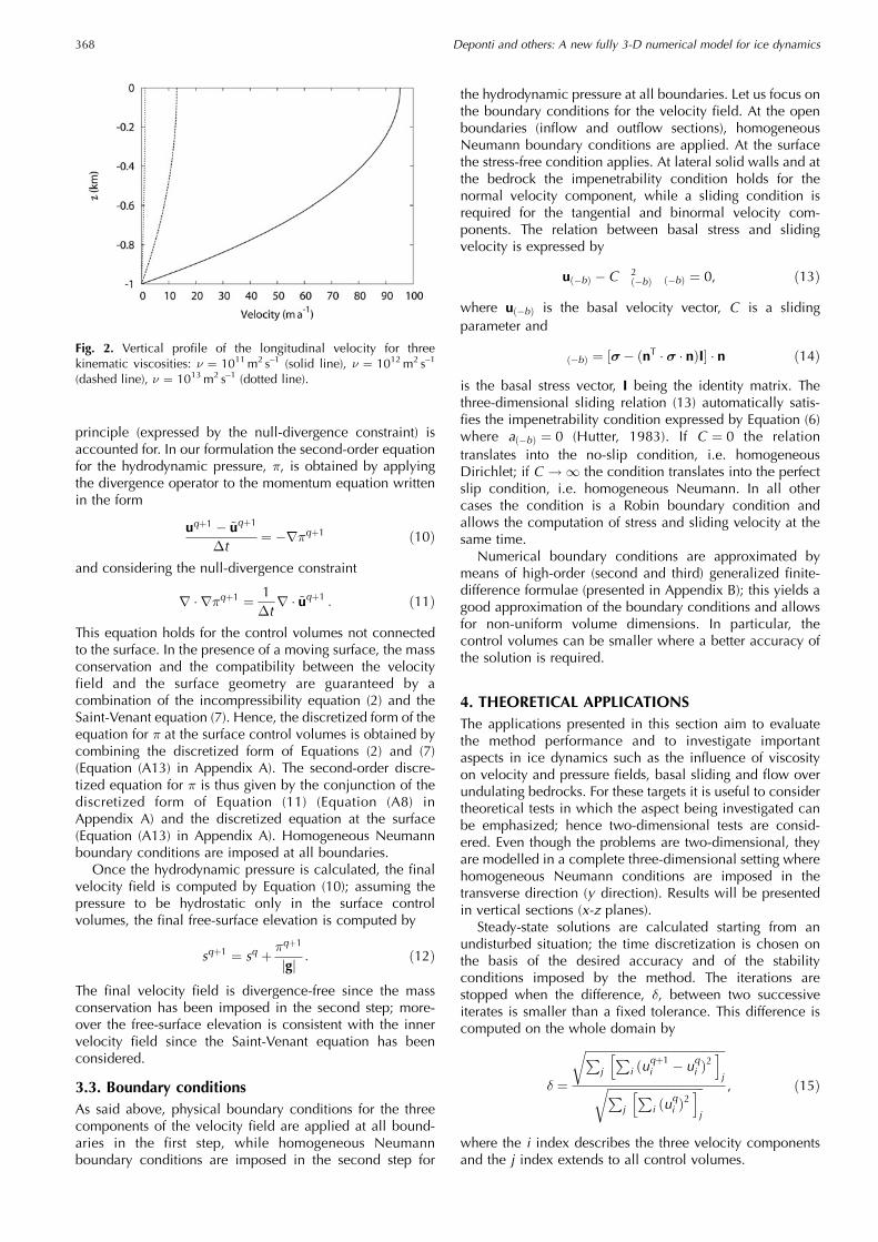
Fig. 8. (a) Discretized bedrock geometry, (b) free surface, (c) velocity field in the central longitudinal section (y ¼ 3000m), (d) surfacevelocity field, (e) hydrodynamic pressure field in the central longitudinal section and (f) effective stress �e in the central longitudinal sectionof case B of the application to Priestley Glacier. The components of the gravity acceleration vector in the considered reference system aregx ¼ 0:170, gy ¼ 0:012, gz ¼ �9:809 (see section 3.1). Pressure and velocity fields are strongly affected by the bedrock geometry and arefully three-dimensional; variations in all directions are evident. The surface undulations are of the same amplitude as the measured ones. Thestress is maximum at the base and minimum at the surface.

Deponti and others: A new fully 3-D numerical model for ice dynamics372

The measured surface velocity at P is 81ma–1; thecalculated velocity at the central point of the nearest controlvolume is 77.5ma–1 for case A and 83.8ma–1 for case B.The simulations were performed on a Dell Precision 670equipped with an Intel Xeon 3.4GHz and 2GB RAM. Thetotal time for A simulation was 2.75 hours, while the totaltime for B simulation was 33.8 hours. This increase ofcomputational time is due to the use of an iterative method(the preconditioned biconjugate gradient method) for thesolution of the algebraic systems.

For case A, only surface elevation and velocity field arepresented in Figure 7. For case B, more results are presentedin Figure 8. In all cases the numerical results are in goodagreement with physical values.

6. CONCLUSIONSA numerical model for ice dynamics is presented and tested.The model is based on a fluid-dynamic approach, and istime-evolutive and fully three-dimensional. The full pressurefield is computed by considering both the hydrostatic andhydrodynamic pressure components, all the stresses arecalculated and the velocity field is calculated by applyingboundary conditions at all the domain boundaries (i.e. atsurface, bedrock, lateral walls, inflow and outflow sections).The model uses high-order approximations for field equa-tions and boundary conditions. It can deal with bothconstant and variable viscosity thanks to a constitutive lawbased on Glen’s law. The presented theoretical applicationsinvestigate basal processes such as flow in the presence ofslipperiness variations or of bedrock undulations. The testsshow that the pressure is not always hydrostatic and, inparticular cases, a hydrodynamic pressure component arisesand plays an important role in basal processes and icedynamics. Further investigations of the role of the hydro-dynamic pressure could be of interest and provide importantinformation about ice dynamics.

The application to Priestley Glacier shows the capabilityof the model to deal with real cases, and the importance ofconsidering the three-dimensional Stokes equations in orderto have a good description of ice dynamics where three-dimensional effects are not negligible.

ACKNOWLEDGEMENTSThis work was financially supported by Ministerodell’Istruzione dell’Universita e della Ricerca through theCOFIN Project and by IMONT (Italian National MountainInstitute) through the CryoAlp Project. We thank an anony-mous referee, G.H. Gudmundsson and the scientific editor,J. Meyssonnier, for valuable comments that improved themanuscript.

REFERENCESArmfield, S. and R. Street. 2002. An analysis and comparison of the

time accuracy of fractional step methods for the Navier–Stokesequations on staggered grids. Int. J. Numer. Meth. Fl., 38,255–282.

Baroni, C. 1996. Mount Melbourne Quadrangle (Victoria Land).(Antarctic Geomorphological and Glaciological 1 : 250,000Map Series.) Siena, Museo Nazionale dell’Antartide.

Blatter, H., G.K.C. Clarke and J. Colinge. 1998. Stress and velocityfields in glaciers: Part II. Sliding and basal stress distribution.J. Glaciol., 44(148), 457–466.

Calov, R., A. Savvin, R. Greve, I. Hansen and K. Hutter. 1998.Simulation of the Antarctic ice sheet with a three-dimensionalpolythermal ice-sheet model, in support of the EPICA project.Ann. Glaciol., 27, 201–206.

Casulli, V. 1999. A semi-implicit finite difference method for non-hydrostatic, free-surface flows. Int. J. Numer. Meth. Fl., 30(4),425–440.

Casulli, V. and P. Zanolli. 2002. Semi-implicit numerical modelingof non-hydrostatic free-surface flows for environmental prob-lems. Math. Comput. Model., 36, 1131–1149.

Colinge, J. and H. Blatter. 1998. Stress and velocity fields inglaciers: Part I. Finite-difference schemes for higher-order glaciermodels. J. Glaciol., 44(148), 448–456.

Deponti, A. 2003. Mass and thermal flows in Alpine glaciers.Application to Lys Glacier (Monte Rosa, Italian Alps). (PhDthesis, University of Milano–Bicocca.)

Deponti, A., V. Pennati and L. de Biase. 2004. A 3D FV method forAlpine glaciers. In Sunden, B., C.A. Brebbia and A.C. Mendes,eds. Advanced computational methods in heat transfer VIII.Boston, MA, WIT Press.

Deponti, A., V. Pennati and L. de Biase. 2006. A fully 3D finitevolume method for incompressible Navier–Stokes equations.Int. J. Numer. Meth. Fl. 52(1). (10.1002/fld.1190.).

Gresho, P.M. 1991. Some current CFD issues relevant to theincompressible Navier–Stokes equations. Comput. Method.Appl. M., 87, 201–252.

Greve, R. 1997. A continuum-mechanical formulation for shallowpolythermal ice sheets. Philos. T. Roy. Soc. A. 355(1726),921–974.

Greve, R. and R. Calov. 2002. Comparison of numerical schemesfor the solution of the ice-thickness equation in a dynamic/thermodynamic ice-sheet model. J. Comput. Phys., 179,649–664.

Gudmundsson, G.H. 1997a. Basal-flow characteristics of a linearmedium sliding frictionless over small bedrock undulations.J. Glaciol., 43(143), 71–79.

Gudmundsson, G.H. 1997b. Basal-flow characteristics of a non-linear flow sliding frictionless over strongly undulating bedrock.J. Glaciol., 43(143), 80–89.

Gudmundsson, G.H. 1999. A three-dimensional numerical modelof the confluence area of Unteraargletscher, Bernese Alps,Switzerland. J. Glaciol., 45(150), 219–230.

Gudmundsson, G.H. 2003. Transmission of basal variability to aglacier surface. J. Geophys. Res., 108(B5), 2253. (10.1029/2002JB0022107.)

Guermond, J.-L. and L. Quartapelle. 1998. On stability andconvergence of projection methods based on pressure Poissonequation. Int. J. Numer. Meth. Fl., 26(9), 1039–1053.

Hindmarsh, R.C.A. 2004. A numerical comparison of approxima-tions to the Stokes equations used in ice sheet and glaciermodeling. J. Geophys. Res., 109(F1), F01012. (10.1029/2003JF000065.)

Hubbard, A., H. Blatter, P. Nienow, D. Mair and B. Hubbard. 1998.Comparison of a three-dimensional model for glacier flow withfield data from Haut Glacier d’Arolla, Switzerland. J. Glaciol.,44(147), 368–378.

Hutter, K. 1983. Theoretical glaciology; material science of ice andthe mechanics of glaciers and ice sheets. Dordrecht, etc.,D. Reidel Publishing; Terra Scientific Publishing.

Huybrechts, P. 1990. A 3-D model for the Antarctic ice sheet: asensitivity study on the glacial–interglacial contrast. ClimateDyn., 5(2), 79–92.

Jenssen, D. 1977. A three-dimensional polar ice-sheet model.J. Glaciol., 18(80), 373–389.

Le Meur, E. and C. Vincent. 2003. A two-dimensional shallow ice-flow model of Glacier de Saint-Sorlin, France. J. Glaciol.,49(167), 527–538.

Luthi, M. and M. Funk. 2000. Dating of ice cores from a highAlpine glacier with a flow model for cold firn. Ann. Glaciol., 31,69–79.

Deponti and others: A new fully 3-D numerical model for ice dynamics 373

Luthi, M.P. and M. Funk. 2001. Modelling heat flow in a cold, high-altitude glacier: interpretation of measurements from ColleGnifetti, Swiss Alps. J. Glaciol., 47(157), 314–324.

Mahaffy, M.W. 1976. A three-dimensional numerical model of icesheets: tests on the Barnes Ice Cap, Northwest Territories.J. Geophys. Res., 81(6), 1059–1066.

Mangeney, A., F. Califano and K. Hutter. 1997. A numerical study ofanisotropic, low Reynolds number, free surface flow for icesheet modeling. J. Geophys. Res., 102(B10), 22,749–22,764.

Martın, C., F.J. Navarro, J. Otero, M.L. Cuadrado and M.I. Corcuera.2004. Three-dimensional modelling of the dynamics of JohnsonsGlacier (Livingston Island, Antarctica). Ann. Glaciol., 39, 1–8.

Nye, J.F. 1952. The mechanics of glacier flow. J. Glaciol., 2(12),82–93.

Paterson, W.S.B. 1994. The physics of glaciers. Third edition.Oxford, etc., Elsevier.

Pattyn, F. 2002. Transient glacier response with a higher-ordernumerical ice-flow model. J. Glaciol., 48(162), 467–477.

Pennati, V. and S. Corti. 1994. Generalized finite-differencesolution of 3-D elliptical problems involving Neumann bound-ary conditions. Commun. Numer. Meth. En., 10(1), 43–58.

Pennati, V., L. de Biase and F. Feraudi. 1992. A generalized finite-difference solution of parabolic 3-D problems on multi-connected regions. Communications in Applied NumericalMethods, 8(6), 361–371.

Ritz, C., A. Fabre and A. Letreguilly. 1997. Sensitivity of aGreenland ice sheet model to ice flow and ablation parameters:consequences for the evolution through the last glacial cycle.Climate Dyn., 13(1), 11–24.

Schoof, C. 2002. Basal perturbations under ice streams: form dragand surface expression. J. Glaciol., 48(162), 407–416.

Van der Veen, C.J. 1989. A numerical scheme for calculatingstresses and strain rates in glaciers.Math. Geol., 21(3), 363–377.

Van der Veen, C.J. and I.M. Whillans. 1989. Force budget: I. Theoryand numerical methods. J. Glaciol., 35(119), 53–60.

APPENDIX AIn this appendix the space and time discretization of theproposed scheme is presented in detail.

In Figure 1 a sketch of a three-dimensional controlvolume is presented. Although the control volumes arelabeled at their central points with a proper number (as inthe finite-element method), for clarity in this paper eachcontrol volume is labelled by the three indices ijk of itscentre. Faces 1 and 2 of the control volume are orthogonalto the x axis, faces 3 and 4 to the y axis and faces 5 and 6 tothe z axis.

In the first step the discretized component-wise form ofEquation (9) is solved:

~uqþ1ijk �zqijk �

�t�xijk

X2f¼1

�qijk

@~uqþ1

@x

� �ijk�zqijknx

" #f

� �t�yijk

X4f¼3

�qijk

@~uqþ1

@y

� �ijk�zqijkny

" #f

��tX6f¼5

�qijk

@~uqþ1

@z

� �ijknz

" #f

¼ uqijk�zqijk þ�t�zqijk �jgj @sq

@x

� �ijþ gx þ @uq

@x� r�q

� �ijk

" #,

ðA1Þ

~vqþ1ijk �zqijk �

�t�xijk

X2f¼1

�qijk

@~vqþ1

@x

� �ijk�zqijknx

" #f

� �t�yijk

X4f¼3

�qijk

@~vqþ1

@y

� �ijk�zqijkny

" #f

��tX6f¼5

�qijk

@~vqþ1

@z

� �ijknz

" #f

¼ vqijk�zqijk þ�t�zqijk �jgj @sq

@y

� �ijþ gy þ @uq

@y� r�q

� �ijk

" #,

ðA2Þ

~wqþ1ijk �zqijk �

�t�xijk

X2f¼1

�qijk

@ ~wqþ1

@x

� �ijk�zqijknx

" #f

� �t�yijk

X4f¼3

�qijk

@ ~wqþ1

@y

� �ijk�zqijkny

" #f

��tX6f¼5

�qijk

@ ~wqþ1

@z

� �ijknz

" #f

¼ wqijk�zqijk þ�t�zqijk jgj þ gz þ @uq

@z� r�q

� �ijk

" #: ðA3Þ

The sums are extended over the control volume faces, �½ �frefers to quantities calculated on a control volume face,and nx , ny , nz are the components of the outward vectornormal to each control volume face. Details on theapproximation of the diffusive term on control volumefaces are presented in Appendix B. The superscriptsrepresent the time indices; as said above, the dimension�z is time-indexed because it is allowed to vary in time forsurface control volumes. In the computation of the fluxes,�z of faces in common between two surface controlvolumes is calculated by the weighted mean value of the�z of the two control volumes.

In the second step the following discretized form ofEquation (10) is considered:

uqþ1ijk ¼ ~uqþ1

ijk ��t@�qþ1

@x

� �ijk, ðA4Þ

vqþ1ijk ¼ ~vqþ1

ijk ��t@�qþ1

@y

� �ijk, ðA5Þ

wqþ1ijk ¼ ~wqþ1

ijk ��t@�qþ1

@z

� �ijk: ðA6Þ

The discrete incompressibility equation is

1�xijk

X2f¼1

uqþ1ijk �zqijknx

� fþ 1�yijk

X4f¼3

vqþ1ijk �zqijkny

� f

þX6f¼5

wqþ1ijk nz

� f¼ 0: ðA7Þ

Formal substitution of Equations (A4–A6) into Equation (A7)

Deponti and others: A new fully 3-D numerical model for ice dynamics374

gives the discrete equations for the hydrodynamic pressure,�qþ1, for the volumes not connected to the free surface:

�t1

�xijk

X2f¼1

@�qþ1

@x

�ijk�zqijknx

( )f

þ 1�yijk

X4f¼3

@�qþ1

@y

�ijk

�zqijkny

( )f

þX6f¼5

@�qþ1

@z

�ijk

nz

( )f

!

¼ 1�xijk

X2f¼1

~uqþ1ijk �zqijknx

n of

þ 1�yijk

X4f¼3

~vqþ1ijk �zqijkny

n ofþX6f¼5

~wqþ1ijk nz

n of,

for k ¼ m, m þ 1, . . . , M � 1, ðA8Þ

where m and M are the k index of the lower and uppercontrol volume layer respectively.

In order to calculate the hydrodynamic pressure, �qþ1, onthe surface control volumes together with the final free-surface elevation, the following discretized form of theSaint-Venant equation (7) is considered:

sqþ1ij ¼ sqij �

XMk¼m

�t�xij

X2f¼1

uqþ1ijk �zqijknx

� f

"

þ �t�yij

X4f¼3

vqþ1ijk �zqijkny

� f

#: ðA9Þ

Formal substitution of Equation (A7) into Equation (A9) gives

sqþ1ij � sqij�t

þ 1�xijM

X2f¼1

uqþ1ijM �zqijMnx

h if

þ 1�yijM

X4f¼3

vqþ1ijM �zqijMny

h ifþ ðwqþ1

ijM �wqþ1ijm Þnz

h if¼5

¼ 0:

ðA10Þ

Formal substitution of the momentum equations (A4–A6)into Equation (A10) gives:

sqþ1ij

�t��t

1�xijM

X2f¼1

@�qþ1

@x

� �ijM

�zqijMnx

" #f

(

þ 1�yijM

X4f¼3

@�qþ1

@y

� �ijM

�zqijMny

" #f

þ @�qþ1

@z

� �ijM

nz

" #f¼5

)

¼sqij�t

� 1�xijM

X2f¼1

~uqþ1ijM �zqijMnx

h if

� 1�yijM

X4f¼3

~vqþ1ijM �zqijMny

h if� ð ~wqþ1

ijM � ~wqþ1ijm Þnz

h if¼5

:

ðA11Þ

In this equation, two unknowns are present: namely the newsurface elevation sqþ1

ij and the hydrodynamic pressure at the

surface control volumes �qþ1ijM . In order to solve this equation,

the pressure in the surface control volumes is consideredhydrostatic, i.e. jgjðsqþ1 � zÞ ¼ jgjðsq � zÞ þ �qþ1, whence

sqþ1 ¼ sq þ �qþ1

jgj : ðA12Þ

Substitution of Equation (A12) into Equation (A11) gives thediscrete equation for �qþ1 in the surface control volumes:

��qþ1ijM

jgj�tþ�t

1�xijM

X2f¼1

@�qþ1

@x

� �ijM

�zqijMnx

" #f

(

þ 1�yijM

X4f¼3

@�qþ1

@y

� �ijM

�zqijMny

" #f

þ @�qþ1

@z

� �ijM

nz

" #f¼5

)

¼ 1�xijM

X2f¼1

~uqþ1ijM �zqijMnx

h ifþ 1�yijM

X4f¼3

~vqþ1ijM �zqijMny

h if

þ ð ~wqþ1ijM � ~wqþ1

ijm Þnzh i

f¼5: ðA13Þ

Finally, the system of discrete equations for �qþ1 is given bythe conjunction of Equations (A8) and (A13).

After the hydrodynamic pressure is calculated, the finalvelocity field is computed by Equations (A4–A6) and thefinal free-surface elevation is computed by Equation (A12).

APPENDIX BIn this appendix the details of the approximation of diffusiveterms on control volume faces and of boundary conditionsare presented.

The approximation of the diffusive flux of the threevelocity components, u, v, w, and of the hydrodynamicpressure, �, on the control volume face requires theapproximation of the first derivative of each quantity onthe control volume face itself; this is done using a four-pointcentred formula; the formula is third-order accurate evenwith non-uniform grid spacing.

As an example, the first derivative, @u=@x, on controlvolume face 1 is presented here. Appropriate rotations andtranslations of the presented scheme allow the approxima-tion of all derivatives on all control volume faces. Applica-tion to the other field variables allows the approximation ofall diffusive fluxes. In order to approximate @u=@x atpoint Pw placed on face 1 (Fig. 1), the stencil presented inFigure 9a is used. The distances of stencil points arecalculated on the basis of a local reference system (�, �, �)in which the origin is placed at point P2. The approximationof @u=@x is

@u@x

�Pw

¼X4i¼1

Diui , ðB1Þ

where ui are the u values to be calculated at points Pi and

Deponti and others: A new fully 3-D numerical model for ice dynamics 375

the Di coefficients are

D1 ¼ �234�1ð�1 þ �3Þð�1 þ �4Þ ,

D2 ¼ � 1�3

� �34�1�4

,

D3 ¼ �4�1�3 � 3�23 þ 4�1�4 þ 4�3�44�3ð�1 þ �3Þð�4 � �3Þ ,

D4 ¼ �234�4ð�3 � �4Þð�1 þ �4Þ :

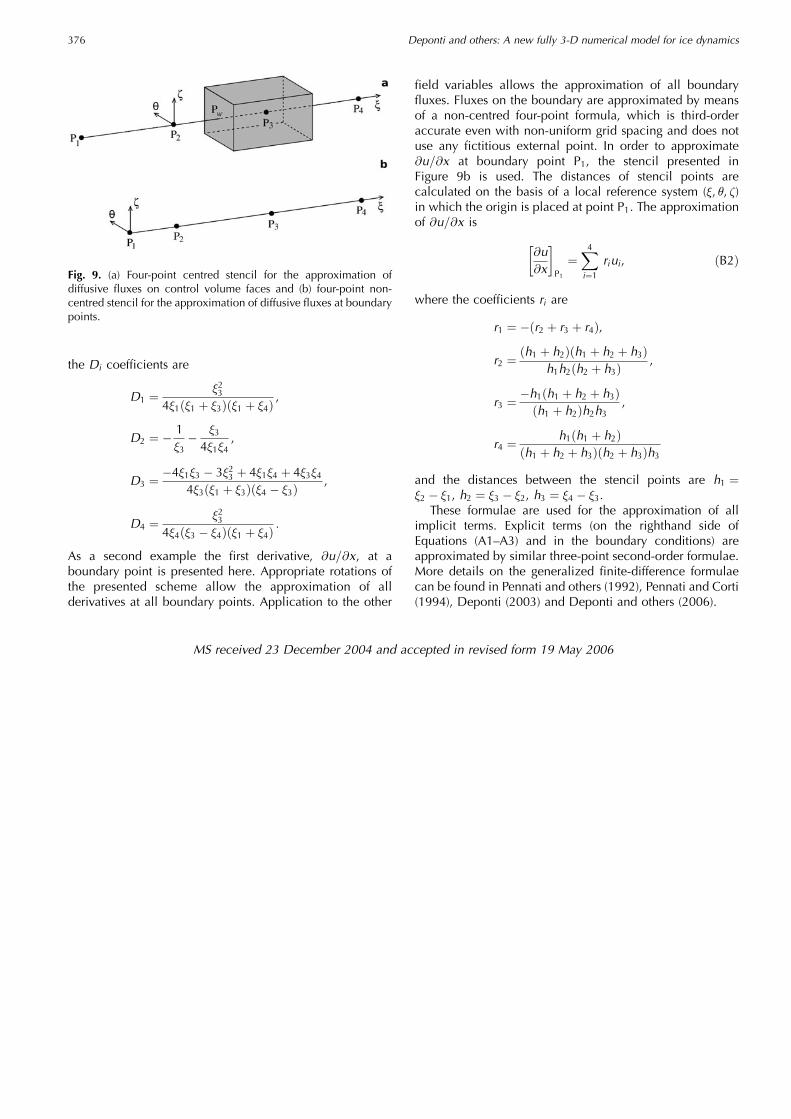
As a second example the first derivative, @u=@x, at aboundary point is presented here. Appropriate rotations ofthe presented scheme allow the approximation of allderivatives at all boundary points. Application to the other

field variables allows the approximation of all boundaryfluxes. Fluxes on the boundary are approximated by meansof a non-centred four-point formula, which is third-orderaccurate even with non-uniform grid spacing and does notuse any fictitious external point. In order to approximate@u=@x at boundary point P1, the stencil presented inFigure 9b is used. The distances of stencil points arecalculated on the basis of a local reference system (�, �, �)in which the origin is placed at point P1. The approximationof @u=@x is

@u@x

�P1

¼X4i¼1

riui, ðB2Þ

where the coefficients ri are

r1 ¼ �ðr2 þ r3 þ r4Þ,

r2 ¼ ðh1 þ h2Þðh1 þ h2 þ h3Þh1h2ðh2 þ h3Þ ,

r3 ¼ �h1ðh1 þ h2 þ h3Þðh1 þ h2Þh2h3 ,

r4 ¼ h1ðh1 þ h2Þðh1 þ h2 þ h3Þðh2 þ h3Þh3

and the distances between the stencil points are h1 ¼�2 � �1, h2 ¼ �3 � �2, h3 ¼ �4 � �3.

These formulae are used for the approximation of allimplicit terms. Explicit terms (on the righthand side ofEquations (A1–A3) and in the boundary conditions) areapproximated by similar three-point second-order formulae.More details on the generalized finite-difference formulaecan be found in Pennati and others (1992), Pennati and Corti(1994), Deponti (2003) and Deponti and others (2006).

MS received 23 December 2004 and accepted in revised form 19 May 2006

Fig. 9. (a) Four-point centred stencil for the approximation ofdiffusive fluxes on control volume faces and (b) four-point non-centred stencil for the approximation of diffusive fluxes at boundarypoints.

Deponti and others: A new fully 3-D numerical model for ice dynamics376