82

A new global tactical asset allocation approach to implement in a global macro hedge fund

Juan LAbordA HerreroAbante Asesoresricardo LAbordA HerreroIbercaja

Abstract: We present a new Global Tactical Asset Allocation (GTAA) approach to implement in a Global Macro Hedge Fund, taking into account the modern portfolio theory. The methodology we introduce is based on new advanced analytics, which will give us a clear advantage to exploit opportunities, in a period where the indexed household wealth growth will be low and the active management will be needed. First, we propose state variable selection using classification and regression trees. Second, we detail a novel approach to estimate optimal portfolio weighs without explicitly modelling the underlying return distribution. Finally, we will apply a procedure to reduce the risk of high losses, proposing a coherent measure of risk: the expected loss exceeding value at risk (Conditional VaR).

Key Words: Global Tactical Asset Allocation (GTAA), Global Macro Hedge Fund, Classification and Regression Trees, Optimal Parametric Weight, Conditional Value at Risk (CVaR).

Título: Un nuevo enfoque dentro la Asignación Global Táctica de Activos: Implementación de un Global Macro Hedge Fund

resumen: Presentamos un nuevo enfoque de Asignación Global Táctica de Activos aplicable a la creación de un Global Macro Hedge Fund, que incorpora la teoría moderna de formación de carteras. Nuestra metodología basada en herramientas de análisis cuantitativo nos posibilita explotar las oportunidades del mercado, en un periodo en el que el crecimiento de la riqueza de los consu-midores será reducido y un management activo será especialmente valorado. Primero, proponemos la elección de las variables de estado relevantes mediante la clasificación y regresión por árboles (CART). Segundo, detallamos un nuevo enfoque para estimar la relación entre las variables de estado y los pesos óptimos de los activos, que consideramos en un contexto long/short por pares de activos, sin necesidad de modelizar la distribución de rendimientos de los activos subyacentes. Finalmente, aplicamos un método para asignar la riqueza del fondo entre las apuestas tácticas long/short, que reduce el downsiderisk ó riesgo de grandes pérdidas, utilizando una medida coherente de riesgo: la pérdida esperada más allá del VaR (CVaR).

Palabras claves: Asignación Global Táctica de Activos, Global Macro Hedge Fund, Clasificación y Árboles de Regresión, Selección dinámica de activos, Función de utilidad CRRA, CVaR.

JeL código: G11

Nota: Trabajo recibido el 10 de diciembre 2008. Aceptado el 30 de enero 2009

83

Colaboración

A N

ew G

loba

l Tac

tical

Ass

et A

lloca

tion

App

roac

h to

...

Colaboración

1. INTrodUCTIoN

The development of a financial literature focused on the time varying nature of asset returns and the ample evidence that these asset returns are predictable has motivated the increase of the portfolio advice related to the market timing and the influence of the time horizon on optimal porfolios. One of the consequences of this new modern portfolio theory has been the spectacular growth of the hedge fund industry in recent years, becoming the primary source of active manage-ment, specially when best managers are forming hedge funds. However that raises the question whether they have become so large that they have eliminated the opportunities they are seeking to exploit. Although opportunities are disappearing fastest where hedge funds are very active, and where the same trading rules have been used for some time, opportunities remain ample where there are fewer hedge funds, or where funds use new trade rules, property information, or advanced analytics.

We will focus in this paper in the field of models for alpha generation, proposing a new and original Global Tactical Asset Allocation (GTAA) approach to implement in a Global Macro Hedge Fund. The methodology we propose is based on new advanced analytics, which will give us a clear advantage to exploit opportunities, in a period where the indexed household wealth growth will be low and the active management will be needed.

The GTAA’s objective is to obtain better-than-benchmark returns, the target alpha, as well as a “classic” or benchmark-plus products (S&P 500 + 6%) or as absolute return or Euribor-plus prod-ucts (example: EURIBOR 3 months + 10%), but with, possibly, lower-than-benchmark volatility. That means minimize tracking error. Although our methodology is included in the Global Tactical Asset Allocation techniques, however it is a novel approach to dynamic portfolio selection with clear advantages we will detail. There are three steps. First we propose state variable selection us-ing classification and regression trees. Second we detail a novel approach related to a very recent literature (Brandt and Santa Clara (2006), Brandt, Santa Clara, and Valkanov (2007)) on drawing inferences about optimal portfolio weighs without explicitly modelling the underlying return distribution. We will model directly the portfolio weight in each of our asset pairs as a function of the bet’s predictors. The coefficients of this function are found by optimizing the investor’s aver-age utility of the portfolio return over the sample period. That implies the achievement of high Information Ratios but taking into account higher order moments of the excess return distribution (skewness and kurtosis), related to downside risks. Finally we will apply an approach to reduce the risk of high losses, proposing a coherent measure of risk: the expected loss exceeding value at risk (Conditional VaR).

This document is organised as follows. Section 2 details an overview of our new GTAA approach. Section 3 develops the state variables selection, through classification and regres-sion trees, that we will use as predictors in each of our asset pairs. Section 4 presents an ap-proach on drawing inferences about optimal portfolio weights without explicitly modelling the underlying return distribution (Brandt, Santa Clara and Valkanov (2007)). We will model directly the portfolio weight in each of our asset pairs as a function of the bet’s predictors. Section 5 gives an approach to reduce the risk of high losses and allocate the initial wealth among the different tactical bets, proposing a coherent measure of risk: the expected loss exceeding value at risk or CVaR (Rockafellar and Uryasev, (2001)). Section 6 sums up the main conclusions.

84

2. AN oVerVIeW oF A NeW GLobAL TACTICAL ASSeT ALLoCATIoN APProACH To IMPLeMeNT IN A GLobAL MACro HedGe FUNd

In this section we will focus on the philosophy of our GTTA approach, detailing the GTAA investment process in practice, previously to explain in the following sections the three steps of our methodology.

2.1. GTAA Philosophy: from Research to Investment

The philosophy of the methodology we propose rest on the following basic principles:

• The consistent application of modern portfolio theory provides a fundamental discipline for asset allocation.

• Markets with improving economic climate, trading below fundamental value, and favourable market conditions tend to outperform.

• Investment decisions should be based on forward looking views.• Excess return analysis is the key to performance measurement.• Global efficiency should be currency and benchmark independent.• We will measure and test strategies. On-going research into current and new strategies.

The analytical quant approach we propose will be applied to our fundamental analysis on valuation, economic climate and behavioral finance. The purpose is to understanding the stable dynamic which drives each asset pair, calculating the different bets’ size, extrapolating the final target alpha which could be our objective for different constant relative risk aversion (CRRA) levels, and reducing the risk of high losses or black swan. But what do valuation, economic climate, and market climate mean?

Value provides long information horizon, and is the most consistently rewarded strategy over the long term. Market pressure acts to return markets back to equilibrium.

Economic climate will give us medium information horizon. Value is not enough because market can remain over or undervalued for long periods of time. In this sense, economic condi-tions affect the speed with which markets return to fundamental value. We will use only financial variables which will provide us information about economic cycle, modeling market respond to these financial variables. We will not forecast them.

Market climate provides short term information. Markets are not always rational, and investors behavior and sentiment produce markets over-and undershooting, and could affect the speed with which markets return to fundamental value. There are informed investors that lead the market. Market prices dynamic and changes and revisions in expectations provide the climate information.

2.2. GTAA in practice

Our GTAA investment process in practice is based on the following basic principles:

i-. All the forecasts to compute will be made on asset pairs.

85

Colaboración

A N

ew G

loba

l Tac

tical

Ass

et A

lloca

tion

App

roac

h to

...

Our dependent variable is the 1 month forward excess returns, for every asset pair, at the end of each month. Our predictive variables are ordered variables and they are relevant for excess return prediction in financial literature. There is a large number of possible inputs, which then required various algorithms to reduce the inputs to a manageable and relevant number. For better capturing the dynamic of the models, we propose to use the predictive variables well known in the literature in levels but also in momentum, defined as the variation of the variable on 3 and 12 months: Dividend yield Short term/long term interest rates, the slope of the Yield Curve, Credit Spreads, Earning Yield/Bond Yield,Earnings/Dividends ratio, Momentum and mean reversion dynamics, Book to market, Idiosyncratic volatility, Skew, VIX, Gold, oil and commodity prices, Small versus large performance, Value versus growth performance, Transportation and utilities versus industrial or index performance.

ii.- We will add a reasonably number of bets

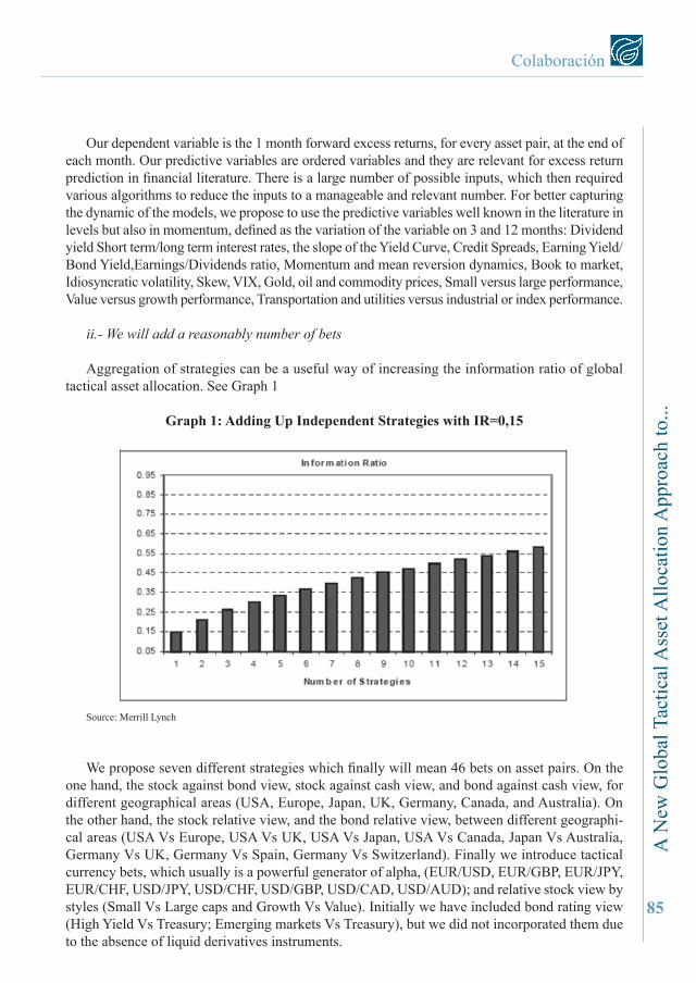
Aggregation of strategies can be a useful way of increasing the information ratio of global tactical asset allocation. See Graph 1

Graph 1: Adding Up Independent Strategies with Ir=0,15

Source: Merrill Lynch

We propose seven different strategies which finally will mean 46 bets on asset pairs. On the one hand, the stock against bond view, stock against cash view, and bond against cash view, for different geographical areas (USA, Europe, Japan, UK, Germany, Canada, and Australia). On the other hand, the stock relative view, and the bond relative view, between different geographi-cal areas (USA Vs Europe, USA Vs UK, USA Vs Japan, USA Vs Canada, Japan Vs Australia, Germany Vs UK, Germany Vs Spain, Germany Vs Switzerland). Finally we introduce tactical currency bets, which usually is a powerful generator of alpha, (EUR/USD, EUR/GBP, EUR/JPY, EUR/CHF, USD/JPY, USD/CHF, USD/GBP, USD/CAD, USD/AUD); and relative stock view by styles (Small Vs Large caps and Growth Vs Value). Initially we have included bond rating view (High Yield Vs Treasury; Emerging markets Vs Treasury), but we did not incorporated them due to the absence of liquid derivatives instruments.

86

iii.- The use of futures as investment tools.

The implementation will be made through futures and forwards to minimize transaction costs. In this sense, we must take into account that a long future bet is equivalent to a hedge tactical bet, that is, to a long position in the asset and a short one in the cash of that asset market. So, the dependent variable will be the difference between excess returns of each asset over the cash of its market.

iv.- The distribution of the optimal portfolio weights changes with the level of risk aversion.

Not surprisingly, the differences in the optimal portfolio weights translate into equally striking differences in the distribution of the optimized portfolio (average returns, volatility, alpha, and information ratio): they decrease with the investor’s level of risk aversion.

3. STATe VArIAbLeS SeLeCTIoN USING CLASSIFICATIoN ANd reGreSSIoN TreeS

In this section we introduce the state variables selection, through classification and regression trees, that we will use as predictors in each of our asset pairs.

Given the statistical characteristics of financial series, Laborda (2004) proposed a methodol-ogy that allowed us to accurately forecast the relative returns of financial assets and to implement tactical asset allocation (TAA) strategies, as part of a basic portfolio management model (equities, bonds and cash). They focused on that line of investigation which, with the implication of predict-ability in series of returns, allows us, on the basis of fundamental variables, to exploit the set of information that these offer in order to segment and classify homogenous areas, on the basis of which we can predict higher returns from one asset relative to another. The proposed technique was classification and regression trees. Once the forecast relative returns are calculated, a TAA system is developed from which they derive the structure of the optimal aggressiveness factors of the various tactical strategies, which allowed us, using a benchmark portfolio, to calculate the weightings to hold in each of the assets.

The relevant features of this approach are described as follow. First, input variable weights should be allowed to vary with time. Moreover, the relative influence of each input variable should depend on its interrelation with other variables, defining non-linear dynamic system. Second, the non-linear algorithm should identify homogeneous zones for the relative returns, relevant for our analysis, using the predictor variables to split the sample and define these homogeneous zones. Third, in a sequential process the algorithm chooses the input variable with higher discrimination power for each tree primary node. In addition, is repeated to identify secondary homogeneous zones.

The method that best suits these main guidelines is part of a global set of models of pattern recognition, and it is called “Classification and Regression Trees”. Regression trees are used to forecast the number of elements in each of the different homogeneous zones of a categorical vari-able, using one or more predictive variables. Consequently they are very useful to explain and/or forecast the responses of the dependent categorical variable, and have a lot in common with traditional methods of discriminant and cluster analysis or with more sophisticated techniques as non-linear and non-parametric estimation.

87

Colaboración

A N

ew G

loba

l Tac

tical

Ass

et A

lloca

tion

App

roac

h to

...

Although all the classification methods already described produce optimal classifiers, the main advantage of the regression trees methodology is that allow us also to have an overview of the predic-tive structure of the problem. They accomplish all the properties common to general classification models (precision, intuitive structure, unbiased inference and quick learning) incorporating also two additional characteristics very attractive for our purpose: flexibility and hierarchical structure. This hierarchy is estimated in the form of binary trees that produces combinations that reduce the dimensionality of the data and improve the predictive capacity. The tree is a set of “if-then clauses” that guide us to better understanding the decision problem. Thus, there are two essential elements in regression trees: the input variable thresholds and decision equation. An additional advantage of this methodology comes from their dynamic structure, and their capacity to analyse separately the impact of one variable impact at the time” t”, and not only the global effect. Furthermore, it is easy to exploit additional information from new variables or additional categories. Finally, clas-sification trees can be used for continuous, categorical or mixed predictors. The main references for this literature are Breiman et al. (1984), Loh y Shih, (1997), y Gehrke y Loh (1999).

The results as part of a basic portfolio management model (equities, bonds and cash) are spectaculars. But what happens if we have not only 3 asset pairs but 46 as in our case. The in-stability problem of CART, that is, small variations on learning sample may produce different trees, is more difficult to solve with so many bets. But the main disadvantage has to do with the traditional approach to optimizing portfolios in a two step process: first modelling the joint distribution of returns, excess returns or alphas; second solving for the corresponding optimal portfolio weights. That is not only difficult to implement for a large number of assets or asset pairs, but also yields notoriously noisy and unstable results. On the one hand, in a alpha-T.E. framework that means estimating for each date t a large number of tN conditional expected alphas and ( ) 22 tNtN + conditional variance an covariance of alphas. On the other hand, besides the fact that the number of these moments grow quickly with the number of bets, making robust estimation a real problem, it is extremely challenging to parameterize the covariance matrix of alphas in a way that guarantees its positive definiteness. Furthermore, extending the traditional approach beyond first and second moments is practically impossible because it requires modelling not only the conditional skewness and kurtosis of each asset or asset pairs, but also the numerous higher- order cross-moments.

We propose a new methodology for solving these problems. We will model directly the port-folio weight in each of our asset pairs as a function of the best’s predictors. The coefficients of this function are found by optimizing the investor’s average utility of the portfolio return over the sample period. That implies the achievement of high Information Ratios but taking into account higher order moments of the excess return distribution (skewness and kurtosis), related to downside risks. Finally we will apply an approach to reduce the risk of high losses, proposing a coherent measure of risk: the expected loss exceeding value at risk (Conditional VaR). Previously we will select the state variables, through classification and regression trees, that we will use as predictors in each of our asset pairs. We will justify and detail how to do that.

3.1. Heuristic Search Modeling Systems (CART and QUEST) in Model Input Selection

Model input selection is the process of choosing the input variables that will be used to create a model for making predictions and arriving at recommendations. We must solve the following trade-off: adding inputs gives the model more things to consider, but extra variables can confuse and

88

dilute the outcomes. In this sense the number of required examples for uncorrelated inputs grows exponentially with the number of input variables. This is termed the “curse of dimensionality”. Since practical experience clearly shows that paring down the number of inputs often results in models that are more accurate, it is necessary to find sound ways to reduce the quantity of candi-date inputs. To assist in this searching process several automated strategies have been developed, including among others Exhaustive Search, Ordered Search, Genetic Search, and Heuristic Search.

Exhaustive Search is too slow for more practical situations and runs the risk of overfitting by building myriad models.

Ordered Search involves systems like forward selection and backward elimination, which are often employed with multiple linear regression. One variation is the stepwise regression, which is a combination of forward and backward searches, and can either add or remove variables at any given stage of the search. For nonlinear problems these searches fail to find good combinations of inputs.

Genetic Search is a procedure driven by genetic algorithms and although they are very good finding useful combinations of inputs, required more stringent testing to unsure they have not ac-cidentally stumbled onto a bad solution which merely looks good.

Heuristic Search modeling systems, as CART and QEST, perform their own input selection as part of the modeling process, and can be operated either on their own or as variable selectors for other modeling systems. In this sense CART help build models that isolate the most important variables. One of the great strengths of CART is its ability to pick out the significant variables, even when they are hidden among hundreds or thousands of irrelevant variables. This is the procedure we have chosen using to that the STATISTICA software package from StatSoft.

In Laborda and Munera (2000) there is a description of the basic regression trees structure and the construction of classification trees. Basically, CART generates a binary decision tree based on yes/no answers and produces nodes until it has created the largest tree that fits the data. This ensures that the node-generating process is not halted too soon and important structures are not overlooked. Upon creating the structure, the system prunes back the tree and uses a self-test procedure to ensure that the model is not over-fitting. This produces a smaller optimal-sized tree. A sum-up of the decision trees algorithm component can be seen in table 1. For more details see Laborda and Munera (2000).

Table 1. Algorithm Components of a decision Tree.

1. Criteria to measure the Accuracy of the Forecast.• Misclassification costs.

2. Splitting Rule: • CART (Breiman et alt 1984)• QUEST (Loh and Shih 1997)• Others: CHAID, GUIDE, C45, RANDOM FORESTS…

3. Stopping Rule. • Minimum number of cases• Fraction of cases

4. Pruning Rule:• Replacement error method• Cross-validation error• Cost-Complexity reduction

89

Colaboración

A N

ew G

loba

l Tac

tical

Ass

et A

lloca

tion

App

roac

h to

...

In order to understand how that works to pick out the significant explanatory variables, we will see two examples of our final 46 bets on asset pairs: Stock against Bonds in USA, and small caps vs large caps. Tables 2 and 3 show final state variables selected in these bets.

Table 2: Final State Variables Selected Using CArT for Stock Vs bonds USA. Predictor variable importance ranking using Univariate splits.

Variable Level

Earning yield/Bond yield (EYG) 99

Slope of Yield Curve 86

Skew Momentum 88

Credit spread 90

EYG Momentum 100

Gold Momentum 73

VIX Momentum 82

0 low importance; 100 high importance

Table 3: Final State Variables Selected Using CArT for Small caps vs Large caps. Predictor variable importance ranking using Univariate splits.

Variable Level

Lagged return 83

Spread High yield vs 10 Y 93

Slope of Yield Curve 81

EUR/USD Momentum 85

G7 Equity Momentum 83

VIX Momentum 81

Fed rate 100

0 low importance; 100 high importance

This selection of predictors are not only based on the level of importance of each state variable, which refers to the individual explanation, in terms of powerful forecasts, of t+1 forward excess returns for the bet. We will take into account the tree obtained by CART: the relative influence of each input variable should depend on its interrelation with other variables, defining a non–linear dynamic system. Although there could be some individual state variable with higher ranking im-portance, the final state variables chosen depends on its interrelation with other variables to define a non-linear dynamic using CART. Let us to explain this using the first example.

90

Graph 2: Final Tree Using CArT for Stock Vs bonds USA.

In graph 2 we can see the final tree for the asset pair bet of Stock against Bond in USA, using

• CART splitting rule, • fraction of cases of 0.10 as stopping rule, • FACT-style pruning rule, and misclassification costs to measure accuracy of forecasts.

Variables 8, 5, and 14 refer to earning yield/bond yield, credit spreads, and yield curve levels, respectively, while variables 21, 26, 38, has to do with skew, gold and earning yield/bond yield momentum. Taking into account the importance level for the possible state variables, and this final tree, we finally select the state variables of the table 2.

4. LoNG/SHorT STrATeGIeS: oPTIMAL PArAMeTrIC WeIGTHS

After the Classification and Regression Tree has determined the crucial state variables in each of our asset pairs, the next step in our approach to create a macro hedge fund is to parameterize, in a long/short context, the portfolio weight as a function of the bet’s predictors1 (Brandt, Santa Clara and Valkanov (2007)). The coefficients are found by optimizing the investor’s average utility of the portfolio return over the sample period chosen.

1 We obtain 46 different parametric weights linked to the 46 tactical bets we’ve considered.

91

Colaboración

A N

ew G

loba

l Tac

tical

Ass

et A

lloca

tion

App

roac

h to

...

Given a tactical bet on Assets 1 and 2, the investor’s problem is to choose the portfolio weight, tAssetbetAsset ,2/1α , to maximize the conditional expected utility of the portfolio return, 1, +tpr :

( )[ ] ( )( )[ ]2,11,12/11, 1

,arg/ AssettlAssettAssetbetAssetfttpt RRrUErUEMaxtelallrelativosm +++ −++= αα (1)

where fr is the return of the risk free asset and Asset 1 and 2 have return 2,11,1 , AssettAssett RR ++

We parameterize the optimal portfolio weights as a function of the state variables, tZ , fol-lowing a simple linear specification (Brandt, Santa Clara and Valkanov (2007)).

( ) ββαα '

,2/1 ; tttAsssetbetAsset ZZ == (2)

We assume that the coefficientsβ are constant through the time, what means that the coef-ficients that maximize the investor’s conditional expected utility also maximize the investor’s unconditional expected utility. This implies that we can rewrite the the problem (1) as the following unconditional optimization with respect to the coefficientsβ

( )[ ] ( )( )( )[ ]2,11,1

´1, 1 AssettAssetttftp RRZrUErUEMax +++ −++= ββ (3)

We can estimate the coefficientsβ by maximizing the corresponding sample analog.

( ) ( )( )( )2,11,1´

1

01,

1

0111

AssettAssetttf

T

ttp

T

tRRZrU

TrU

TMax ++

−

=+

−

=

−++= ∑∑ ββ (4)

The maximum expected utility estimate∧

β defined by the optimization problem (3), with the linear portfolio problem (2) satisfies the first order conditions:

( ) ( )( )( ) ( )( )( ) 011;,12,11,1

´2,11,1

´1

0

'1

01 =−−++= ++++

−

=

−

=+ ∑∑ AssettlAssetttAssettAssetttf

T

t

T

ttt RRZRRZrU

TZrh

Tββ (5)

and can therefore be interpreted as a method of moments estimator. From Hansen (1982), the asymptotic covariance matriz of this estimator is

[ ]∑ −−∧

=

=

ββ

111 GVGT

AsyVaR T (6)

92

where

( ) ( ) ( )( ) ( )( )'1;,12,11,1

'1

02,11,1

'1,

''1

0

1AssettAssettt

T

tAssettAssettttp

T

t

tt RRZRRZrUT

ZrhT

G ++

−

=+++

−

=

+ −−=∂

∂= ∑∑ β

β (7)

and V is a consistent estimator of the covariance matriz of ( )β;, Zrh

Assuming that marginal utilities are uncorrelated we can consistently estimate V by:

∑−

=

∧

+

∧

+

1

11 ';,;,1 T

ttttt ZrhZrh

Tββ (8)

We assume that the investor’ utility funcion is isoelastic or CRRA,

( )γ

γ

−=

−+

+ 1

11

1t

tW

WU

whereγ is the investor’s relative risk aversion coefficient. It’s important to outline that the optimization takes into account the relation between the state variables and the expected returns, variances, and even higher order moments, to the extent that they affect the distribution of the optimized portfolio’s returns and therefore the investor’s expected utility of the investor. (Brandt, Santa Clara and Valkanov (2007)).

Using monthly data of the state variables and the asset returns from january 1987 through December 2007, we estimate the coefficients of the optimal portfolio weights for each of our as-set pairs as a function of the state variables, following the linear specification (2), by solving the investor’s problem (3). Given different levels of risk aversion coefficients, , and the 46 different tactical bets, we solve 46 long/short problems: the GMM estimator provides us the estimate ∧

β for each different tactical bet, giving us 46 simple and effective portfolio long/short rule.

We provide two examples of this methodology. The first example consists of determining the optimal parametric weight between Stocks and Bonds. So, Asset 1=Stock and Asset 2=Bonds. The CART has chosen the following state variables as the more important in the relative return Stock/Bond (Table 2): Earning Yield/Bond Yield (EYG), Slope of the Yield Curve 10 Y-3 m, Credit Spread, the three month EYG momentum, the three month Skew momentum, the three month Gold momentum, the three month VIX momentum. The table 4 shows the estimated model: on the one hand, the EYG level and momentum and the Skew momentum has a positive impact on the optimal stock vs bond allocation; on the other hand, the slope of the yield curve and the increase of the uncertainty proxied by the VIX momentum has a negative impact on the optimal stock vs bond allocation.

93

Colaboración

A N

ew G

loba

l Tac

tical

Ass

et A

lloca

tion

App

roac

h to

...

Table 4

This table shows estimates of the long/short portfolio policy between stocks and bonds, optimized for a power utility with different relative risk aversion coefficients.:

where EYG is the 12 month Earning yield forward/Bond Yield (Yield of T-Note), R10Y-R3m is the slope of the yield curve, CS is the level of the spread high yield vs TIR 10 años, MEYG is the three month EYG momentum, MSkew is the three month Skew momentum, MGold is the three month Gold momentum, CVIX is the three month VIX momentum.The sample period is from jan 1987 through nov 2007 .

EYG R10y-R3m CS MEYG MSkew Mgold CVIX2 5.83 -1.06 -0.97 3.84 7.56 4.54 -1.80

t-est. (5.07) (-2.96) (-1.05) (2.61) (1.79) (0.93) (-2.55)5 2.97 -0.54 -0.48 1.96 3.96 2.53 -0.93

t-est. (5.13) (-3.02) (-1.05) (2.74) (1.89) (1.02) (-2.75)10 1.99 -0.36 -0.32 1.32 2.68 1.74 -0.63

t-est. (5.13) (-3.02) (-1.05) (2.74) (1.89) (1.02) (-2.75)15 1.50 -0.27 -0.24 0.99 2.03 1.33 -0.47

t-est. (5.13) (-3.02) (-1.05) (2.74) (1.89) (1.02) (-2.75)20 1.00 -0.18 -0.16 0.66 1.36 0.90 -0.32

t-est. (5.13) (-3.02) (-1.05) (2.74) (1.89) (1.02) (-2.75)40 0.75 -0.14 -0.12 0.50 1.03 0.68 -0.24

t-est. (5.13) (-3.02) (-1.05) (2.74) (1.89) (1.02) (-2.75)

Table 5

This table shows estimates of the long/short portfolio policy between small and large caps, optimized for a power utility with different relative risk aversion coefficients.:

where Fed is the Fed level of interest rate, HY is the level of the spread high yield vs TIR 10 años, EUR/USD is the three month change of the dollar vs the Euro, CVIX is the one month change of the VIX, RVG7 is the three month change of a G7 Equity Index, R10Y-R3m is the slope of the yield curve and Ret is the one month lagged Russell 2000 vs S&P 500 return.The sample period is from january 1987 through november 2007 .

Fed HY EUR/USD CVIX RVG7 R10y-R3m Ret2 -2.08 7.22 -43.49 0.55 24.08 -0.49 -35.16

t-est. (-3.31) (2.29) (-2.51) (0.15) (1.85) (-0.33) (-2.75)5 -0.90 3.22 -18.23 0.12 10.43 -0.31 -13.85

t-est. (-3.49) (2.44) (-2.65) (0.08) (1.94) (-0.5) (-3.07)10 -0.46 1.67 -9.22 0.04 5.33 -0.18 -6.82

t-est. (-3.85) (2.51) (-2.70) (0.05) (1.98) (-0.56) (-3.21)15 -0.31 1.13 -6.16 0.02 3.58 -0.12 -4.51

t-est. (-3.61) (2.53) (-2.71) (0.04) (1.99) (-0.59) (-3.26)20 -0.23 0.85 -4.63 0.01 2.69 -0.09 -3.37

t-est. (-3.63) (2.55) (-2.72) (0.03) (2.01) (-0.6) (-3.29)40 -0.12 0.43 -2.32 0.01 1.35 -0.05 -1.67

t-est. (-3.66) (2.57) (-2.73) (0.02) (2.02) (-0.63) (-3.33)

94

The second example consists of determining the optimal parametric weight between small caps and large caps (Asset 1=small caps and Asset 2=large caps). We assume that the Russel 2000 and the S&P 500 are a good proxy of the small caps and large caps universe. The CART has chosen the following state variables as the more important in the small caps/large caps relative return (Table 3): the Fed rate, the level of the spread high yield vs 10 Y Note, the three month USD/EUR momentum, the one month change of the VIX, the three month G7 Equity Index momentum, the slope of the yield curve and the one month lagged Russell 2000 vs S&P 500 return . The table 5 shows that the level of the Fed rate, the depreciation of the USD vs Euro, a positive lagged Rus-sell 2000 vs S&P 500 return and a negative G7 equity index momentum have a negative impact on the small caps vs large caps allocation given the long/short approach; the level of spread high yield vs 10 Y Note has a positive impact on the small caps allocation.

5. CoNdITIoNAL VALUe AT rISK oPTIMIZATIoN oF LoNG/SHorT STrATeGIeS

The last step to create our Macro Hedge Fund is to determine the allocation of the initial wealth among the differents long/short strategies. Given each of our asset pairs, the CART al-lowed us to infer the crucial state variables driving the relative return of two assets; the approach of optimal parametric weights was used to determine the relation between the state variables and the N different long/short strategies. This section deals with the problem of finding an optimal combination of the N “optimal” different long/short strategies found in the previous section . We choose to minimize the CVaR, also called mean excess loss, (Rockafellar and Uryasev, (2001)), which is a suitable approach given the high number of tactical bets we consider.

Following Rockafellar and Uryasev (2001), let ( )yxf , the loss associated with the decision vector nRx∈ and the random vector mRy∈ . The vector x can be interpreted as the portfolio of the “optimal” long/short strategies, with X as the set of available portfolios. The vector y stands for the uncertainties that can affect the loss. The underlying probability distribution of mRy∈ will be assumed for convenience to have a density, we denote by ( )yp .

The probability of ( )yxf , not exceeding a threshold α is

(9)

As a function of α , and given a fixed nRx∈ , ( )αψ ,x is the cumulative distribution func-tion for the loss associated with x. It’s fundamental in determining the VaR and the CVaR. The VaR and the CVaR, with respect to a probability level ( )1,0∈β , VaR−β and the ,CVaR−βwill be denoted by

( ) ( ){ }βαψααβ ≥∈= ,:min xRx (10)

95

Colaboración

A N

ew G

loba

l Tac

tical

Ass

et A

lloca

tion

App

roac

h to

...

(11)

It’s posible the characterization of ( )xβα and ( )xβφ in terms of the next function, defined on RX × , which plays a crucial role (Rockafellar and Uryasev (2001)).

(12)

where 0, >=+ ttt and 0,0 <=+ tt

Rockafellar and Uryasev, (2001) show that as a function of α , ( )αβ ,xF is convex and continuosly differentiable. The CVaR−β or the loss associated with the vector nRx∈ is

( ) ( )αφ βαβ ,min xFxR∈

= (13)

Rockafellar y Uryasev (2001) also show that minimizing the CVaR−β of the loss associated with x over all Xx∈ , is equivalent to minimize ( )αβ ,xF over all the ( ) RXx ×∈α, in the sense that

( )( )

( )αφ βαβ ,minmin,

xFxRXxXx ×∈∈

= (14)

This equivalence let us minimize the CVaR−β using linear programming techniques applied to the function ( )αβ ,xF (Rockafellar and Uryasev (2001)); we will find the optimal portfolio x associated to the long/short strategies and the VaR which minimizes the CVaR given a confidence level β and the restrictions described below.

In order to evaluate the losses related to a portfolio Xx∈ , we consider the historical returns, which we denote by jy , delivered by the j=1....N “optimal” long/short strategies which follow the rules described in the previous section, originating the vector ( )Nyyyy ,...., 21= . The return on a portfolio x is the sum of the returns on the “optimal” long/short bets. The loss, being the negative of this is given by

( ) [ ] yxyxyxyxyxf TNN −=+++−= ......, 2211

(15)

Given our historical sample set qyyy ,...., 21 , we can approximate the function ( )αβ ,xF , by

96

( ) [ ]∑=

+≈

−−

+=q

kk

T yxq

xF1)1(

1, αβ

ααβ (16)

In terms of auxiliary variables ku for k=1...r, it is equivalent to minimizing the linear expres-sion (Rockafellar and Uryasev (2001))

∑=−

+q

kku

q 1)1(1β

α (17)

subject to

rkuyxu kkT

k ,....1,0,0 =≥++≥ α (18)

Njx j ,...1,0 =≥ (19)

11

=∑=

N

jjx (20)

( ) Rx ≥µ (21)

The expressions (19), (20) and (21) mean that the optimal weights are not negative, sum up to one and deliver an expected return larger or equal than R (the desired target).

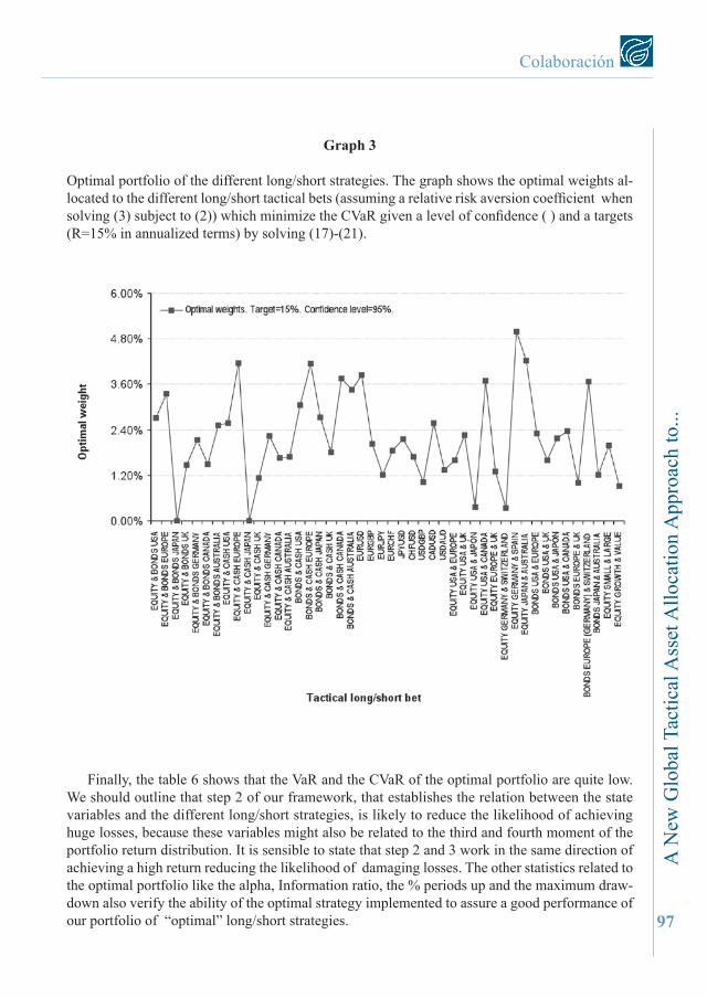
We provide an example of this methodology: we choose the optimal portfolio of the different long/short strategies which minimizes the CVaR given a level of confidence ( ) and a target (R=15% in annualized terms) by solving the problem (17)-(21). The graph 3 shows, assuming in the step 2 a relative risk averion coefficient of 10, the optimal weights of the 46 bets which minimize the CVaR of the portfolio. The bets are related to the seven different strategies we consider: the stock against bond view, stock against cash view, bond against cash view, the stock relative view, and the bond relative view, between different geographical areas, currency bets and relative stock view by styles. We observe that the optimal weigths allocated to the long/short strategies do not deliver extreme solutions, so all of them may offer a good diversification against downside risk.

97

Colaboración

A N

ew G

loba

l Tac

tical

Ass

et A

lloca

tion

App

roac

h to

...

Graph 3

Optimal portfolio of the different long/short strategies. The graph shows the optimal weights al-located to the different long/short tactical bets (assuming a relative risk aversion coefficient when solving (3) subject to (2)) which minimize the CVaR given a level of confidence ( ) and a targets (R=15% in annualized terms) by solving (17)-(21).

Finally, the table 6 shows that the VaR and the CVaR of the optimal portfolio are quite low. We should outline that step 2 of our framework, that establishes the relation between the state variables and the different long/short strategies, is likely to reduce the likelihood of achieving huge losses, because these variables might also be related to the third and fourth moment of the portfolio return distribution. It is sensible to state that step 2 and 3 work in the same direction of achieving a high return reducing the likelihood of damaging losses. The other statistics related to the optimal portfolio like the alpha, Information ratio, the % periods up and the maximum draw-down also verify the ability of the optimal strategy implemented to assure a good performance of our portfolio of “optimal” long/short strategies.

98

Table 6

This table shows the VaR and the CVaR of the optimal portfolio assuming and target (R=15% in annualized terms). It also shows other statistics of the optimal portfolio.

Confidence level=95%VaR 1,99%

CVaR 2,16%Annualized return 15%

Annualized Volatility 5,10%Alpha 9,92%

Tracking error 5,14%Information Ratio 1.93

Periods up%/down% 87,21%/12,79%Maximum Drawdown 14,13%

6. CoNCLUSIoN

We deal with the problem of creating a Global Macro Hedge Fund which considers a large number of possible tactical bets. Our procedure consists of three steps: 1) First, we propose a state variable selection using classification and regression trees. 2) Second, we model directly the portfolio weight in each of our asset pairs as a function of the bet’s predictors (Brandt, Santa Clara, and Valkanov (2007)). 3) Finally, we apply an approach to combine the different long/short strategies focused in reducing the risk of high losses: minimize the expected loss exceeding value at risk (Conditional VaR) given a confidence level (Rockafellar and Uryasev (2001)). A framework that could integrate steps 2 and 3 is required for future research.

7. reFereNCeS

Brandt, M., Santa Clara P., 2006, Dynamic Portfolio Selection by Augmenting the Asset Space, The Journal of Finance Vol LXI, Nº 5, 2187-2216.Brandt, M., Santa Clara P., Valkanov R., 2007, Parametric portfolio policies: exploiting character-istics in the cross section of equity returns, Proximamente Review of Financial Studies.Breiman, L., et al. (1998): Classification And Regression Trees. Chapman & Hall / CRC Press.Gehrke, J., and Loh, W.-Y. (1999): Data Mining with Decision and Regression Trees. KDD1999 Tutorial.Hansen, L., 1982, Large sample properties of Generalized Method of Moments estimators. Econo-metrica, 50, 1029-1054.Laborda, J., and Munera, A. (2001): “Tactical Asset Allocation with Classification and Regression Trees”. Proceedings Eight International Conference Forecasting Financial Markets: Advances for Exchange Rates, Interest Rates and Asset Management.Laborda, J. (2004): “Colocación Táctica de Activos y Estrategias Long-Short con Árboles de Clasificación.” Revista de Economía Financiera, Diciembre, 84-114.Loh, W.-Y., and Shih, Y.-S. (1997): “Split Selection Methods for Classification Trees”. Statistica Sinica, 7, 815-840.Rockafellar, R.T, Uryasev, S., 2001, “Optimization of conditional value at risk”, journal of Risk, 2.3 (Spring 2000), 21-41.