Page 1
A New Tool for Rock Mass Discontinuity Mapping from Digital Images: VTtrace
Alfred Vinod Antony
Thesis submitted to the faculty of the Virginia Polytechnic Institute and State University in partial fulfillment of the requirements for the degree of
Master of Science In
Civil Engineering
Dr. Joseph E. Dove Dr. Marte S. Gutierrez Dr. Matthew Mauldon
25 April 2005 Blacksburg, Virginia.
Keywords: Automated Fracture Mapping, Rock Mass Characterization, Digital Imaging, Digital Image Processing
Page 2
Rock Mass Discontinuity Trace Detection Using VTtrace
Alfred Vinod Antony
ABSTRACT
Manual fracture mapping in tunnels, caverns, mines or other underground spaces is a
time intensive and sometimes dangerous process. A system that can automate this task could
minimize human exposure to rockfalls, rockbursts or instabilities and facilitate the use of new
methods of data visualization such as virtual environments. This research was undertaken to
develop VTtrace; a semi-automatic fracture mapping algorithm based on image processing
and analysis techniques. Images of a rock exposure surface are made using a “prosumer”
grade digital camera. The grayscale images are preprocessed to remove color information
and any noise or distortion. The smoothed images are converted into binary images. The
binary images are then thinned to extract the fracture map. The fractures are then
separated and stored as different images. Fracture properties such as the length, width,
orientation and large-scale roughness are determined using photogrammetric techniques.
Results from test images shows the VTtrace is effective in extracting rock discontinuity
traces. Additional enhancements to the program are proposed to allow feature attributes
from the three-dimensional surface to be determined.
Page 3
iii
Acknowledgements The author wishes to express his ultimate gratitude to the Almighty for giving an
opportunity to work and complete this research.
The author presents a bouquet of thanks and appreciation to his advisor, Dr.
Joseph E. Dove, for his guidance, encouragement, and support throughout the research
and for the intensive review of the thesis.
The author is also grateful to:
Dr. Marte S. Gutierrez, for giving him the opportunity to work on this research
project and for his kind cooperation and support during the research.
Dr. Matthew Mauldon for his guidance and advice.
His wife, Veena Jose for her love, support and encouragement.
His associates, Jeramy Decker, Sotirios Vardakos and Imsoo Lee for their support
and friendship.
A special thanks to National Science Foundation for funding this research project.
Finally, the author expresses his sincere thanks to Virginia Tech for providing all
the facilities, infrastructure and research friendly environment.
Page 4
iv
Table of Contents
Chapter 1 Introduction..................................................................................................... 1
1.1 Motivation & Objective ...................................................................................... 1
1.2 Terminology........................................................................................................ 2
1.3 Application of Digital Image Processing and Analysis Techniques................... 2
1.4 Organization and structure.................................................................................. 2
Chapter 2 Review of Previous Related Research ............................................................ 4
Chapter 3 Overview of Imaging and Image Processing .................................................. 9
3.1 Early Cameras and Image Formation ................................................................. 9
3.1.1 Cameras with Lenses ................................................................................ 10
3.1.2 Digital Cameras ........................................................................................ 10
3.1.3 Image Representation................................................................................ 11
3.2 Image Processing Operations............................................................................ 13
3.2.1 Smoothing ................................................................................................. 13
3.2.2 Thresholding ............................................................................................. 14
3.2.3 Edge Detection.......................................................................................... 16
3.2.4 Thinning.................................................................................................... 19
Chapter 4 Detection of Rock Mass Discontinuity Traces ............................................. 20
4.1 Imaging Acquisition and Equipment ................................................................ 21
4.2 Image Processing Overview ............................................................................. 21
4.2.1 Smoothing ................................................................................................. 22
4.2.2 Thresholding ............................................................................................. 23
4.2.3 Thinning.................................................................................................... 24
4.2.4 Fracture Separation ................................................................................... 30
4.2.5 Fracture Properties .................................................................................... 31
4.3 Programming platform and User Interface ....................................................... 32
Chapter 5 Test Cases and Results.................................................................................. 38
5.1 Image Smoothing Algorithm ............................................................................ 38
5.1.1 Methodology............................................................................................. 38
5.2 Thresholding Algorithm.................................................................................... 44
Page 5
v
5.3 Thinning Algorithm .......................................................................................... 51
5.3.1 Methodology............................................................................................. 51
5.3.2 Results....................................................................................................... 51
5.3.3 Discussion................................................................................................. 51
5.4 Feature characterization algorithm ................................................................... 63
5.5 Integration Testing ............................................................................................ 66
5.5.1 Methodology............................................................................................. 66
5.5.2 Results....................................................................................................... 66
5.5.3 Discussion................................................................................................. 66
Chapter 6 Conclusions and Recommendations ............................................................. 71
6.1 Recommendations for Future Enhancements ................................................... 71
Chapter 7 References..................................................................................................... 73
Page 6
vi
List of Figures Figure 3.1 Illustration of a pinhole camera…...………………………………………....9
Figure 3.2. Illustration of the Perspective Projection model. .......................................... 10
Figure 3.3. A grayscale image and its histogram…...…………………………………...12
Figure 3.4. Various box filters. ....................................................................................... 13
Figure 3.5. Result of the 5X5 Linear smoothing operation . ........................................... 14
Figure 3.6. Examples of thresholding..………..…...…………………………………...15
Figure 3.7. Intensity plot for a single row of pixels......................................................... 17
Figure 3.8. Illustration of the edge detection operation.………………………………...18
Figure 4.1. Sequence of processes to extract the fracture map……………………..…...20
Figure 4.2. AMADEUS rock mass imaging system. ....................................................... 21
Figure 4.3. Illustration of a 3X3 window median filter………………………………....23
Figure 4.4. Four possible arrangements of pixels……….……………………………....25
Figure 4.5. Numbering sequence of neighborhood pixels……………………………....25
Figure 4.6. Example of Hilditch's crossing number calculation...……………………....26
Figure 4.7. Example of pixel configuration for extreme cases….……………………....28
Figure 4.8. Additional examples of pixel configuration for extreme cases..…………....28
Figure 4.9. Neighborhood pixels while identifying nodes……………………………....30
Figure 4.10. Examples of nodes………………….……….……………………………..30
Figure 4.11. Direction in which the trace width is determined...……………………......31
Figure 4.12 Illustration of large scale roughness calculation .......................................... 32
Figure 4.13 Screen capture of the user interface.............................................................. 33
Figure 4.14. Screen Capture of the User Interface with a test image open...................... 34
Figure 4.15. Screen Capture of the User Interface with a test image after smoothing. ... 35
Figure 4.16 Screen Capture of the User Interface with a test image after thresholding. .. 36
Figure 4.17 Screen Capture of the User Interface with a test image after thinning.......... 37
Figure 5.1. Original Image made in natural light conditions. Note the regions with lichen
growth resulting in tonal differences. ....................................................................... 40
Figure 5.2. After a single pass of the 3X3 median smoothing algorithm. ....................... 40
Figure 5.3. After two passes of the 3X3 median smoothing algorithm. .......................... 41
Figure 5.4. After three passes of the 3X3 median smoothing algorithm. ........................ 41
Page 7
vii
Figure 5.5. After four passes of the 3X3 median smoothing algorithm. ......................... 42
Figure 5.6. After five passes of the 3X3 median smoothing algorithm............................ 42
Figure 5.7. Image with artificial “Salt and Pepper” noise. .............................................. 43
Figure 5.8. Smoothed Image with the “Salt and Pepper” noise removed......................... 43
Figure 5.9. Binary image with threshold value of 150 after single pass 3X3 median
smoothing.................................................................................................................. 45
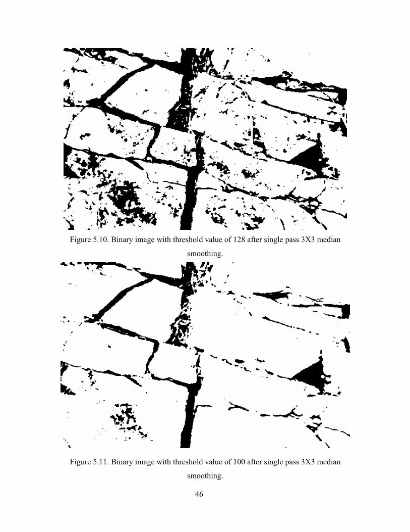
Figure 5.10. Binary image with threshold value of 128 after single pass 3X3 median
smoothing.................................................................................................................. 46
Figure 5.11. Binary image with threshold value of 100 after single pass 3X3 median
smoothing.................................................................................................................. 46
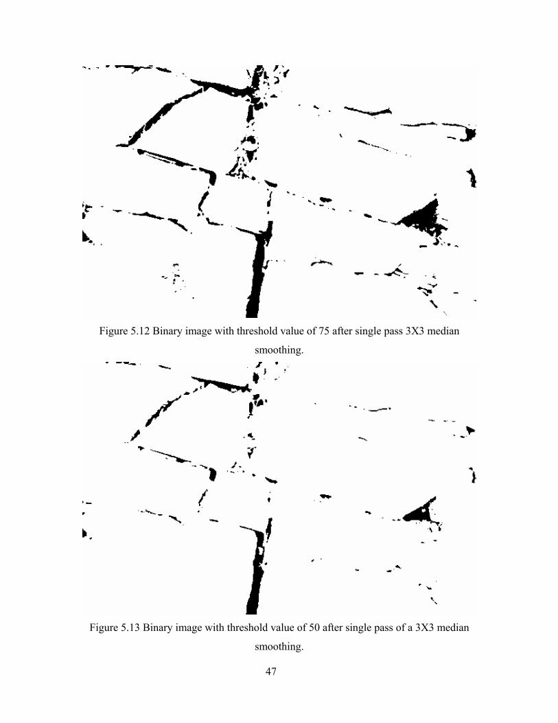
Figure 5.12 Binary image with threshold value of 75 after single pass 3X3 median
smoothing.................................................................................................................. 47
Figure 5.13 Binary image with threshold value of 50 after single pass of a 3X3 median
smoothing.................................................................................................................. 47
Figure 5.14 Binary image with threshold value of 128 after five pass 3X3 median
smoothing.................................................................................................................. 48
Figure 5.15 Binary image with threshold value of 100 after five pass 3X3 median
smoothing.................................................................................................................. 48
Figure 5.16. Binary image with threshold value of 150 without smoothing. ................... 49
Figure 5.17. Binary image with threshold value of 128 without smoothing. ................... 49
Figure 5.18. Binary image with threshold value of 100 without smoothing. ................... 50
Figure 5.19. Binary image with threshold value of 50 without smoothing. ..................... 50
Figure 5.20. Thinned image using Hilditch’s algorithm after single pass 3X3 smoothing
and threshold of 150.................................................................................................. 52
Figure 5.21. Thinned image using Hilditch’s algorithm after single pass 3X3 smoothing
and threshold of 128.................................................................................................. 53
Figure 5.22. Thinned image using Hilditch’s algorithm after single pass 3X3 smoothing
and threshold of 100.................................................................................................. 53
Figure 5.23. Thinned image using Hilditch’s algorithm after single pass 3X3 smoothing
and threshold of 50.................................................................................................... 54
Page 8
viii
Figure 5.24. Thinned image using Zhang & Suen algorithm after single pass 3X3
smoothing and threshold of 150................................................................................ 54
Figure 5.25. Thinned image using Zhang & Suen algorithm after single pass 3X3
smoothing and threshold of 128................................................................................ 55
Figure 5.26. Thinned image using Zhang & Suen algorithm after single pass 3X3
smoothing and threshold of 100................................................................................ 56
Figure 5.27. Thinned image using Zhang & Suen algorithm after single pass 3X3
smoothing and threshold of 50.................................................................................. 56
Figure 5.28. Thinned image using Hilditch’s algorithm after threshold of 120 without
smoothing.................................................................................................................. 57
Figure 5.29. Thinned image using Hilditch’s algorithm after threshold of 100 without
smoothing.................................................................................................................. 57
Figure 5.30. Thinned image using Zhang & Suen algorithm after threshold of 128 without
smoothing.................................................................................................................. 58
Figure 5.31. Thinned image using Zhang & Suen algorithm after threshold at 100 without
smoothing.................................................................................................................. 58
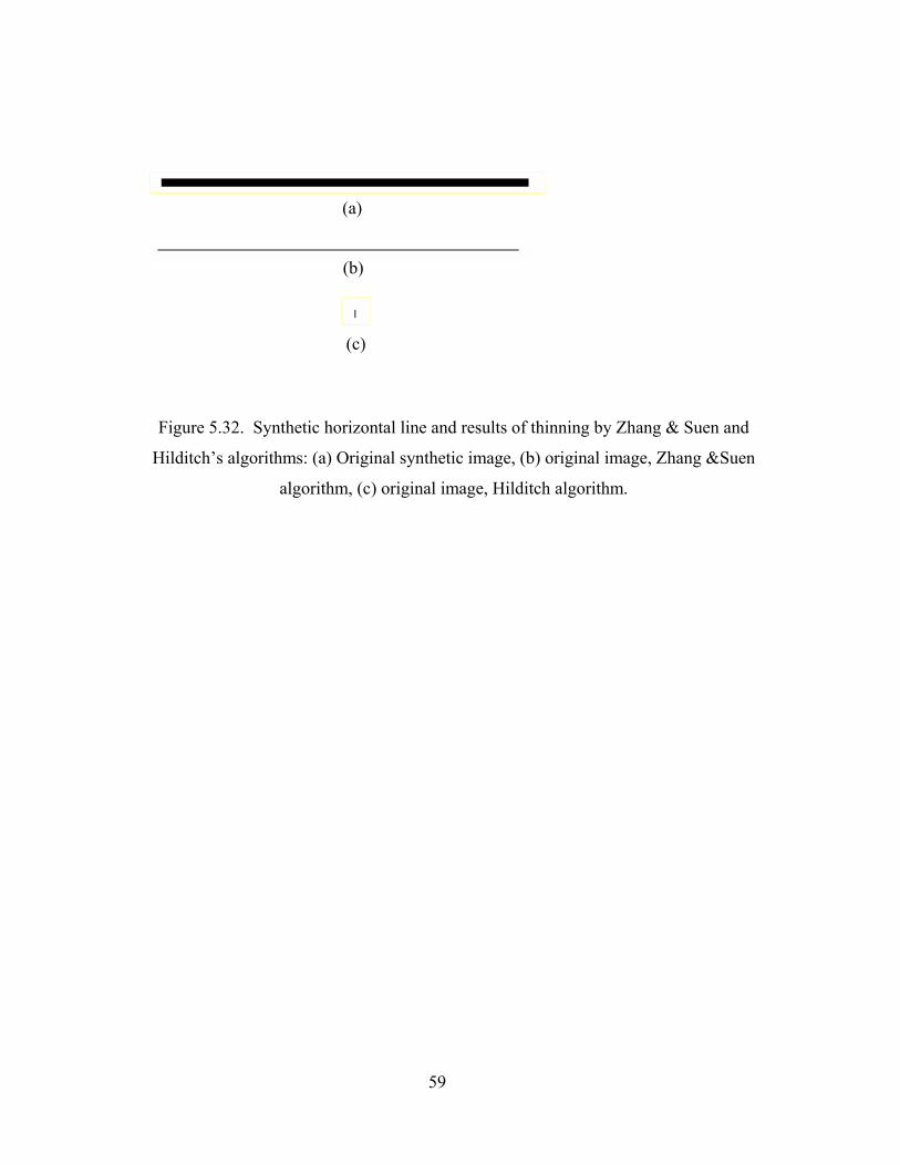
Figure 5.32. Synthetic horizontal line and results of thinning by Zhang & Suen and
Hilditch’s algorithms……………………………………………………………….59
Figure 5.33. Synthetic vertical line and results of thinning by Zhang & Suen and
Hilditch’s algorithms ……..…………………………………………………….….60
Figure 5.32. Synthetic grid pattern and results of thinning by Zhang & Suen and
Hilditch’s algorithms …………….………………………………………………...61
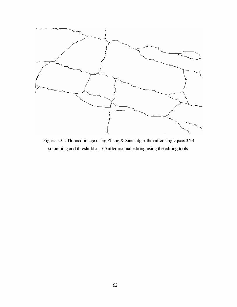
Figure 5.35. Thinned image using Zhang & Suen algorithm after single pass 3X3
smoothing and threshold at 100 after manual editing using the editing tools. ......... 62
Figure 5.36. Original synthetic image and result of the feature characterization
algorithm. .................................................................................................................. 65
Figure 5.37. Original image. ............................................................................................ 67
Figure 5.38. Results of single pass 3X3 median smoothing filter. .................................. 68
Figure 5.39. Smoothed binary image at threshold value of 100. ..................................... 68
Figure 5.40. Result of the Zhang & Suen thinning method. ............................................ 69
Figure 5.41. Final fracture trace map after some manual editing. ................................... 69
Page 9
ix
Figure 5.42. Individual features with their associated properties. ................................... 70
Page 10
1
Chapter 1 Introduction
Accurately recording the distribution, pattern and attributes of rock mass
discontinuities is an important problem in geoengineering. Fractures, joints and faults
largely control the engineering behavior of rock masses and their intersections can create
deadly rockfall hazards. In addition, there is a need within the geoengineering
community for tools that will allow better storage, retrieval, visualization and use of
discontinuity information.
This thesis presents the research undertaken to develop VTtrace, a semi-automatic
program for rock mass discontinuity trace detection using digital image processing and
analysis techniques. The research is a part of the overall research and development effort
for the project “Adaptive Real-Time Geologic Mapping Analysis and Design of
Underground Space” (AMADEUS) supported by the National Science Foundation.
This chapter highlights the importance of this research, motivation for
accomplishing the work and the problems for which it is intended to solve. A brief
overview of the methodology used is also provided.
1.1 Motivation & Objective
Manually mapping discontinuities on the faces of rock exposures is a time intensive
and sometimes dangerous process. Mapping requires that the geoengineer or geologist be
directly adjacent to a rock face and in the zone of influence for events such as rock falls,
rockbursts or other instabilities. Moreover manual measurements are confined to the area
of reach and thus may not be an accurate representation of the entire surface. There is
also a limitation on the amount of data that can be collected manually due to time and
budget constraints.
By extracting traces and attributes of rock discontinuities from images of the same
rock face made at a safe distance, there will be benefits in terms of safety and
productivity. Digital segmentation and storage of discontinuities and attributes will also
facilitate the use of new methods of data visualization, such as virtual environments.
Therefore such a system has great practical significance to the geoengineering profession
and society at large.
Page 11
2
The objective of this research effort is to develop a semi-automated system to
extract discontinuity traces on rock surfaces using digital processing and analysis
techniques. The system is able to estimate fracture properties such as the length, width,
roughness and orientation.
1.2 Terminology
The term discontinuity as applied to a rock mass refers to faults, joints, fractures
and bedding planes that form abrupt structural boundaries. A joint is a break in the rock
mass, which has not had any noticeable movement or displacement. A fault is a break in
the rock mass that has had noticeable movement or displacement along the break. A
bedding plane is the surface parallel to the surface of deposition (Reid 1998). Bedding
planes are features of sedimentary rocks.
The act of creating a digital representation of a rock mass is referred to as imaging.
An image is the actual digital representation that is available on a storage medium.
Image processing involves sequentially modifying the original image using various
mathematical filters. Much of the work described in this thesis involves image
processing. Image analysis is the quantitative measurement and/or estimation of
parameters or features in the image.
1.3 Application of Digital Image Processing and Analysis Techniques
Digital image processing has been used since early 1920’s. In the 1960’s with the
arrival of digital computers, there was rapid advancement in the algorithms and
methodologies for image processing and analysis. Image processing techniques found
application in various fields like industrial inspection, biomedical engineering, remote
sensing, optical character recognition, metrology and photogrammetry, aid for people
with disabilities and many more. The application of image processing techniques in rock
mechanics has been an area of active research as described in the next chapter.
1.4 Organization and structure
This thesis is divided into six chapters. Chapter 2 examines the literature on
previous work on automated discontinuity trace detection. The literature review is also
compared with this research and the similarities and the uniqueness of this research is
Page 12
3
presented. Chapter 3 gives an introduction to the image processing and analysis concept.
Fundamental concepts of the image processing techniques used in this research such as
thresholding, smoothing, thinning and edge detection are explained in detail. Chapter 4
presents the new methodology for the semi-automated detection of discontinuity traces
using digital images. The proposed imaging system and the algorithm for each process is
outlined. Chapter 5 provides the test cases and results for the new system with different
rock mass images and varying user selected parameters. Conclusions are drawn as to the
success and accuracy of the system. Chapter 6 states the practical problems and
challenges that could be encountered while implementing this system and lists
recommendations for future research.
Page 13
4
Chapter 2 Review of Previous Related Research
The use of digital imaging, image processing and photogrammetry methods as tools
for geological and geomechanical rock characterization is a developing area of research.
Enabling technologies for developing this tool come from the fields of computer science
and geoengineering. By fusing technologies from the fields, methods of characterization
can be developed that add to value and quality of project engineering. This chapter
documents previous research results that were found to the most relevant for developing a
semiautomatic fracture mapping tool.
Several studies have been published regarding fracture mapping and rock mass
characterization of rock surfaces using digital images. Lemy and Hadjigeorgiou (2003)
demonstrated the advantages and use of image analysis techniques for rock mass
characterization. Their approach to this problem was to construct the discontinuity trace
maps with the aid of artificial neural networks. The superfluous segments of the trace
map that do not constitute the discontinuity trace are recognized by the neural network
algorithm and are removed. The final step is to identify and connect segments delineating
the same trace. This is achieved by linking all the recognized segments into a continuous
line representing a discontinuity trace.
Rock mass characterization parameters like the Rock Quality Description (RQD),
discontinuity trace length and discontinuity frequency are determined by implementing
photogrammetric techniques, where a digital elevation map of the rock surface is created.
The neural network algorithm used in this research requires a training database that
contains features expected in the actual images. It was found that the algorithm could not
recognize all features in images, which then required human intervention to complete the
trace map. The use of neural networks for the current research was determined to be
cumbersome with little added value at this time. In addition VTtrace is not intended to be
a fully automatic mapping system, as it is believed that human input is needed. However,
neural networks might possibly be the best solution for developing automatic systems.
Page 14
5
Reid and Harrison (2000) presented a methodology for semi-automatic detection
of discontinuity traces in grayscale digital images of rock mass exposures. This
methodology detects discontinuity traces as individual objects, and by doing so
distinguishes one discontinuity trace from another. Discontinuity trace detection is
achieved by using the concept of 'topographic feature labeling', developed by Reid
(1998), and through the development of a method to link together the curvilinear features
in digital images of rock mass exposures. The basic requirement for the discontinuity
trace is that it must have a different brightness from the intact rock surface. It is evident
that a change in pixel value occurs as a discontinuity is crossed. On either side of the
discontinuity, pixel values change in a continuous manner until the minimum pixel value
is reached. If pixel values are envisioned as a continuous surface, the minimum pixel
values would be located in “ravines”.
By calculating the first and second derivatives, the curvature of a plane normal to
the surface is obtained. As the plane is rotated about the surface normal to itself, the
curvature varies (provided that the surface is neither planar nor spherical). When the
curvature becomes either a maximum or a minimum it is called principal curvature, and
the directions in which this occurs are called principal axes of curvature. These principal
directions are represented by the eigenvectors of a symmetric matrix and are therefore
mutually orthogonal. The local shape of the surface is established by considering the first
and second derivatives of the plane curve in the directions of maximum curvature. A
point on a surface can be assigned a topographic label, such as ravine, ridge, peak or pit
The most important aspect of the Reid and Harrison approach is the separation of
the line segments into different objects. This is accomplished by identifying the ravine
pixels, tracing the line segments formed by connecting the ravine pixels and then labeling
the ravine line segments. A linking algorithm is used to connect gaps in the fracture
traces. However, the selection of end pixels that has to be linked with to another pixel has
to be done manually. Manual selection of the end pixel will become very tedious for
some cases especially when there are many images to be processed. To make this
method truly automatic, an algorithm to connect the loose ends of the line segments is
required.
Page 15
6
Kemeny et al. (2003) studied the use of Digital Imaging combined with laser
scanning technologies for field fracture characterization. This method has been developed
into a commercial software package called “Split FX” marketed by Split Engineering,
Inc. The program is able to use digital images or 3-D laser scanning information. It can
delineate fracture traces, determine joint sets, provide 3-D orientation information for
joints and can perform block analysis.
The fracture traces are delineated from the digital images using a modified Hough
transform. Fractures are then separated into sets using an algorithm developed
specifically for this purpose. Once the fracture sets have been identified, several kinds of
information are determined for each fracture set. The most important is the extraction of
3D orientation from the fracture trace information. 3D fracture information is obtained
with the information acquired from two or more non-parallel faces.
The second method suggested by the authors is to use Lidar laser scanning
technology to acquire the digital elevation map of the field surface. The laser scanner
gives a point cloud from which specific information about the fractures in the rock mass
such as orientation, density, size, spacing, roughness etc. are determined. The digital
images used for the analysis of traces should be taken with the camera set up
perpendicular to the rock wall. Correction for inclined camera view is not incorporated in
this system. The orientations of the fractures can also be calculated using image
processing and photogrammetry techniques. The use of laser scanning technology for
fracture traces is a great advancement but there are concerns over the efficiency of the
laser scanner on wet surfaces and the time required for processing the point clouds. The
laser scanner gives a 3D point cloud from which the trace maps and the 3D mesh is
developed using a statistical model.
It is not possible from the literature published on Split FX to determine how well
the components function and the areas of development are required. It does seem to yield
those parameters and information that are most important to geomechanical
characterization.
Gaich et al. (http://www.ifb.tugraz.at/situ/) developed an "Electronic Imaging
System" to capture high-resolution stereoscopic image for tunnel construction. The
Page 16
7
system uses calibrated rotating color line scan cameras and photogrammetric orientation
principles for 3D site measurements. The system uses images from on-site mapping. Each
image represents a surface area of about 10 m width and 8 m in height. Features, such as
fractures, in the range of a few centimeters can be resolved.
The imaging system consists of two digital CCD-line sensor cameras with 6000
elements mounted on rotating camera heads. These are fixed with a rigid frame on a
vehicle. Rotation of the cameras projects panoramic images onto a cylindrical surface.
This imaging technique and the correct seaming of single image parts is used within the
various components of the application.
The interior orientation of the cameras and the geometry of the imaging set-up are
calibrated in the laboratory. Rigid transformations between the cameras and a world
respective tunnel co-ordinate system are also set. The 3D measurement and
reconstruction is based on the epipolar principal. From the known interior and exterior
orientation of the cameras and the calculation of the corresponding picture points the
object point is reconstructed. The analysis results in a triangulated irregular network
(TIN) map.
Accuracy of the 3D reconstruction depends on proper laboratory calibration of
cameras and imaging set-up in the field, co-ordinates of the geotechnical convergence
marks used for computing the exterior camera orientation being precisely determined,
resolution of the images, image quality, and localization of corresponding points in the
stereo images (automatic and interactive).
An interactive program called GeoEDIT was developed for geomechanical
characterization. It allows the geologist to evaluate structural features of tunnel face
images. Traces of discontinuities, boundaries between different lithologies etc. can be
identified with this tool. To distinguish between different structures in an image,
grouping by a layer concept is adopted and displayed in different colors. Visualization of
the tunnel face can be accomplished by using shutter glasses.
Soole and Poropat (2000) applied photogrammetry methods to highwall
mapping, visualization and landslide assessment. The terrestrial photogrammetry system
is targeted at data collection and mapping requirements for highwall mapping, general
Page 17
8
mine site documentation and validation and interpretation of mine data. The system
developed by the authors has simple field procedures, is capable of making direct
measurements of position in orientation parameters using an integrated GPS, orientation
sensors and digital camera hardware for quick data capture and has easy to use digital
photogrammetry software.
Using the data and digital image of a rock mass a separate commercial program
(SIROJOINT) is used to identify, map, annotate and analyze visible structural features.
With this program, the user can identify and measure the orientation, area and position of
joint faces and joint traces; identify and measure geological features such as bedding
planes, faults etc.; identify dominant joint sets using contoured stereonets of orientation
vectors; classify joints according to orientation; calculate spacing for joint sets and
bedding planes and annotate joints with termination information.
Based on the above previous research, the following points are made regarding
development of VTtrace:
• A practical and easy to use fully automatic detection system may not be possible
at this time. Semiautomatic methods may offer more flexibility for the geologist
or engineer in selection and representation of discontinuities but at a higher time
price.
• Either line scan or prosumer digital cameras are suitable for image collection.
Lidar systems can also be used but are expensive at the present.
• A system that uses 'off-the-shelf' technology has the potential for greater
acceptance in the geoengineering community.
Page 18
9
Chapter 3 Overview of Imaging and Image Processing
This chapter provides the reader with a brief overview of how images are created
and acquired, and a discussion of basic image processing methods. There are numerous
books and papers available on this topic. Technologies for image processing are largely
from the computer science and electrical engineering fields; however, they are used in
many crosscutting applications.
3.1 Early Cameras and Image Formation
The first cameras were known as “pinhole cameras”. Essentially this was a box
with a small hole in one of its sides, and a photographic plate on the opposite side. Rays
of light travel in straight lines from the 3D scene onto the photographic plate Forsyth et
al. (2003). The working of a pinhole camera is schematically illustrated in Figure 3.1
The image in a pinhole camera is formed by light rays that issue from the scene
facing the box. The image is formed by the principle of perspective projection, also
known as “pinhole perspective or “central perspective” projection model (Forsyth et al.
2003). Perspective projection model is illustrated in Figure 3.2. Perspective projection
creates inverted images.
Figure 3.1. Illustration of a pinhole camera.
Pinhole
Photographic Plate
3D Scene
Page 19
10
Figure 3.2. Illustration of the Perspective Projection model.
3.1.1 Cameras with Lenses
There are two major reasons why cameras are equipped with lenses. First, lenses
are used to gather more light than just a single ray as in the pinhole camera. Real
pinholes have a finite size, so each point in the image plane is illuminated by a cone of
light rays subtending a finite solid angle. The larger the hole, the wider the cone and the
brighter the image. However, a larger pinhole produces a blurry image. Shrinking the
pinhole produces sharper images but reduces the amount of light reaching the image
plane and may introduce diffraction effects Forsyth et al. (2003).
The second main reason for using the lens is to keep the picture in sharp focus
while gathering the light from the object. Therefore, the problem with pinhole size is
eliminated.
3.1.2 Digital Cameras
A digital camera is similar to a conventional camera in that it has a series of
lenses that focus light to create an image of an object. But instead of focusing the image
light onto a photo-chromatic film, an electronic sensor is used that converts light to
electrical charges. The image sensor employed by most digital cameras is a charge
coupled device (CCD). A CCD sensor uses a rectangular grid of electron-collection sites
laid over a thin silicon wafer to record a measure of the amount of energy reaching each
of them. Each site is formed by growing a layer of silicon dioxide on the wafer and then
Focal Length, (f)
Optical axis
Object (“scene”) point (3-dimensional)
Line of projection
Image point (2-dimensional)
Image plane
Point of projection
Page 20
11
depositing a conductive gate structure over the dioxide. When light photons strike the
silicon, electron-hole pairs are generated (photo-conversion), and the electrons are
captured by the potential well formed by applying a positive electrical potential to the
corresponding gate. The electrons generated at each site are collected over a fixed period
of time.
The charges stored at the individual sites are moved using charge coupling where
charge packets are transferred from site to site by manipulating 'gate potentials' that
preserve the separation of the packets. The image is read out of the CCD one row at a
time, each row being transferred to a serial output register with one element in each
column. Between two row reads, the register transfers its charges one at a time to an
output amplifier that generates a signal proportional to the charge it receives. This
process continues until the entire image has been read out. It can be repeated 30 times per
second for video applications or at a much slower pace, leaving ample time for electron
collection in low light level applications such as astronomy. The digital output of most
CCD cameras is transformed internally into an analog video signal before being passed to
a frame grabber that constructs the final digital image.
3.1.3 Image Representation
A digital image is a 2-dimensional array of intensity values. Each element in the
array in known as “pixel” (picture element). The position of each element in the array
represents spatial co-ordinates in the scene, and the value of each cell represents the pixel
intensity values or brightness value. Common image sizes are 480 pixels (rows) by 640
pixels (columns) and 512 pixels by 512 pixels. The resolution of the digital image is
related to the physical size of the sensor array within the camera, which is usually
specified in terms of the horizontal and vertical pixels or may be specified as the total
number of pixels.
A histogram is a representation of the distribution of observed pixel values. For an
image, the histogram indicates the number of pixels having a particular value. The
histogram of an image h(i) can be represented as follows:
h(i) =1N
p r,c, i( )c∑
r∑ , (3.1)
Page 21
12
where p(r,c,i) = 0 otherwise
N = Number of pixels.
Usually the division by N is omitted for convenience. Histogram is often used as
an estimate of the probability distribution of image intensities. It does not contain the
information of the position of the pixels. It is commonly assumed to have a Gaussian
distribution. Histogram analysis is used in various image processing operations like
thresholding, edge detection etc. An example of an image histogram is shown in Figure
3.3.
1 if pixel value at (r,c) = i
Figure 3.3. A grayscale image and its histogram.
Page 22
13
3.2 Image Processing Operations
Image processing techniques are applied in various fields such as pattern
matching, quality control in an assembly, special effects, and automated tracking. More
recently image processing techniques have been developed for rock mass fracture trace
mapping. Image processing is conduced in stages and some of most common stages are
explained below.
3.2.1 Smoothing
Images typically have the property that the value of a pixel is usually similar to
that of its neighbor. If the image is affected by noise in the form of dead pixels or other
defects the effects of noise is reduced by replacing the pixel value by the weighted
average value of its neighbors. This process is known as smoothing, blurring or noise
reduction. Various filters can be used to perform this operation. Some of the common
filters, known as box or linear filters, are shown in Figure 3.4
Figure 3.4. Various box filters.
91
•
1 1 1
1 1 1
1 1 1
128
•
1 4 1
4 8 4
1 4 1
251
•
1 1 1 1 1
1 1 1 1 1
1 1 1 1 1
1 1 1 1 1
1 1 1 1 1
Page 23
14
These filters are very popular because of their simplicity. The effect of 5X5
smoothing filter is shown in Figure 3.5.
Figure 3.5. Result of the 5X5 Linear smoothing operation.
3.2.2 Thresholding
Thresholding is the process of converting a gray scale image to binary image. A
binary image is an image in which there can be only two possible pixel values. These are
called the “foreground” and the “background” values. Usually the foreground is black
(value = 1) and background is white (value = 0). The simplest way to make this
conversion is to compare each pixel value in the gray scale image to a fixed threshold
value. If the pixel value is less than the threshold value, then the pixel is assigned to the
foreground and if it is greater than the threshold assign it to background, or vice versa.
If T is the threshold value then:
251
•
1 1 1 1 1
1 1 1 1 1
1 1 1 1 1
1 1 1 1 1
1 1 1 1 1
Page 24
15
INEW r,c( )=1 if I r,c( )≤ T
0 if I r,c( )> T
, (3.2)
where I is pixel value and r and c refer to image matrix row and column, respectively. In
some situations, the conditions may be reversed as follows:
INEW r,c( )=1 if I r,c( )> T
0 if I r,c( )≤ T .
(3.3)
Examples of images with different threshold values are shown in Figure 3.6.
Picking the threshold value is critical, as it will determine the actual image used
for subsequent analysis. A threshold level that captures the features critical to the
application should be used. Possibly the best to ensure the desired image is to manually
enter a threshold value for each image. However there are also automatic ways of picking
the threshold value. One of the most popular methods is known as the “Otsu’s Method”
(Otsu 1969). Otsu’s method assumes that the histogram of the grayscale image is bimodal
with modes representing dark and light areas. The thresholding problem is to pick up the
threshold value, T, separating the two modes of the histogram from each other. Each T
Figure 3.6. Examples of thresholding.
Original Image T = 100 T = 128 T = 205
Page 25
16
determines a variance for the group of values that are less than or equal to T and a
variance for the group of values greater than T. The definition for the best threshold
suggested by Otsu (1969) is that threshold for which the weighted sum of group variances
is minimum. The weights are the probabilities of the respective groups. This method will
be described in detail in following chapters.
3.2.3 Edge Detection
Points in the image where brightness changes rapidly are often called “edges” or
“edge points”. Many different edge detection methods have been developed over the
years. Edge detection begins by plotting the intensity values of a single image row as
shown in Figure 3.7. Change in the intensity values can be detected by estimating the
first derivative of the image intensity. Since it is a single row, the problem is one-
dimensional.
Let f(x) represent the intensity profile, the first derivative is given by:
∂fdx
= lim∆x→0
f x + ∆x( )− f x( )∆x
, (3.5)
and can be approximated as:
∂fdx
=f x + ∆x( )− f x( )
∆x. (3.6)
For a two dimensional image array I(x,y) with a pixel distance of ∆x, the
derivatives can be estimated as follows:
∂Idx
≈f x + ∆x, y( )− f x, y( )
∆x, (3.7)
and
∂Idy
≈f x, y + ∆y( )− f x, y( )
∆y. (3.8)
Page 26
17
Figure 3.7. Intensity plot for a single row of pixels.
For discrete image array I(r,c), if ∆x is the width of one pixel, the derivative can
be expressed as follows:
∂fdx
≈I x + ∆x,y( )− I x,y( )
∆x Ix r,c( )= I r,c +1( )− I r,c( ), (3.9)
where:
Ix r,c( )= I r,c +1( )− I r,c( )can be written asIx r,c( )= I r,c( )⋅ −1+ I r,c +1( )⋅1. This
latter term can be used as the 'mask' for Equation 3.9 and can be rewritten in matrix
notation as: [-1 1].
During the edge detection operation, the mask is moved over the original image
and a new image is created. This process is illustrated in Figure 3.9.
26
76
126
176
226
0 50 100 150
Column Number
Pix
el V
alue
Page 27
18
Some commonly used edge detection filters include:
Sobel Operator
-1 0 1
-2 0 2
-1 0 1
Prewitt
-1 0 1
-1 0 1
-1 0 1
Roberts
1 0
0 -1
Some of the advanced non linear edge detectors are the Gaussian operator, Laplacian of
Gaussian (LoG), Canny edge detectors.
Original image I(r,c) New image Ix(r,c)
Figure 3.8. Illustration of the edge detection operation.
Page 28
19
3.2.4 Thinning
For a wide rock discontinuity, the width of the image element is greater than one
pixel. It is convenient to reduce the width so that subsequent operations are easier and
more accurate. Thinning is the process of reducing the width of an image element to just
a single pixel. The process erases the black pixels such that an object without holes
erodes to minimally connected stroke located equidistance from its nearest boundaries
(Pitas 2000). Minimally connected means that adjacent black pixels share common corner
or side. No single pixel has more than two neighboring pixels. Standard thinning
algorithms proposed by Zhang et al. (1999) and Hildtich (1969) are explained in detail in
the following chapter.
A skeleton or stick figure representation of an object is often used to describe its
structure (Pitas 2000). Sometimes the outcomes of thinning and skeletoning will be
unique but it is not always the case.
Page 29
20
Chapter 4 Detection of Rock Mass Discontinuity Traces
The digital image processing techniques explained in the previous chapter can be
used to generate rock mass discontinuity trace maps. A description of the methodology
and algorithms used in VTtrace are described in this chapter. In the present program, the
length, width, roughness and orientation of the discontinuities in the two-dimensional
image plane are determined from the traces. Continuing work will employ
photogrammetry techniques to determine the fracture attributes such as the true length,
width, roughness and orientation of the discontinuity plane.
The sequence of steps adopted to generate the discontinuity trace map is show in
the flow diagram in Figure 4.1.
Initial Image
Preprocessing (Noise Reduction
Smoothing)
Binarization (Thresholding)
Thinning
Separate individual fractures
Figure 4.1 Sequence of processes to extract the fracture trace map.
Page 30
21
4.1 Imaging Acquisition and Equipment
A schematic diagram showing the configuration of the final imaging system is
shown in Figure 4.2. The system will have two digital cameras, a laser distance meter
and a target projector all mounted on a rigid bar capable of rotating the equipment
through a vertical arc of 180 degrees. A portable computer will be used for image
acquisition, control of the cameras and initial image processing. Currently, for this first
portion of the project, a single “prosumer” grade Nikon D-100 digital camera with a
resolution of up to 6.1 megapixels mounted on a conventional tripod is used to capture
images. This camera uses an 18 – 35mm wide angle lens. In the final system, it is
envisioned that images will made to overlap for stereo matching.
Figure 4.2. AMADEUS rock mass imaging system.
4.2 Image Processing Overview
The captured digital image of a fractured rock mass is converted to a grayscale
image by removal of the color information. The grayscale image is first preprocessed to
remove noise and distortion by the process of smoothing. An algorithm is then used to
threshold the image resulting in a binary image. A threshold value is selected such that
pixels below the threshold value are converted to black and all the pixels above the
threshold value are converted to white. The binary image will have only black or white
pixels. The binary image is then thinned to extract the fracture maps. Capabilities are
Page 31
22
provided so that the fracture maps can be edited and annotated manually with the help of
drawing tools, such as a pencil and an eraser, to remove any unnecessary lines. The
individual fractures on the edited image are then separated from the fracture map and
saved as separate image files. Lastly, the individual fracture attributes like the length,
width, orientation and large scale roughness are determined. Each stage of image
processing is explained in detail in the following paragraphs.
4.2.1 Smoothing
This is the first step of the image processing stage. A non-linear low pass
smoothing filter such as the median filter was implemented to reduce the noise in the
image. Non-linear filters were used since they are very effective and preserve the image
edges and details. The median filter not only smoothes noise in homogenous image
regions but tends to produce regions of constant or nearly constant intensity.
The two-dimensional median filter is defined as:
y(i, j) = med x i + r, j + s( ), r, s( )∈A, i, j( )∈Z 2{ }, (4.1)
where Z2 = Z * Z denotes the rectangular digital image plane. The set A∈Z2
defines the filter window. The border pixels are ignored.
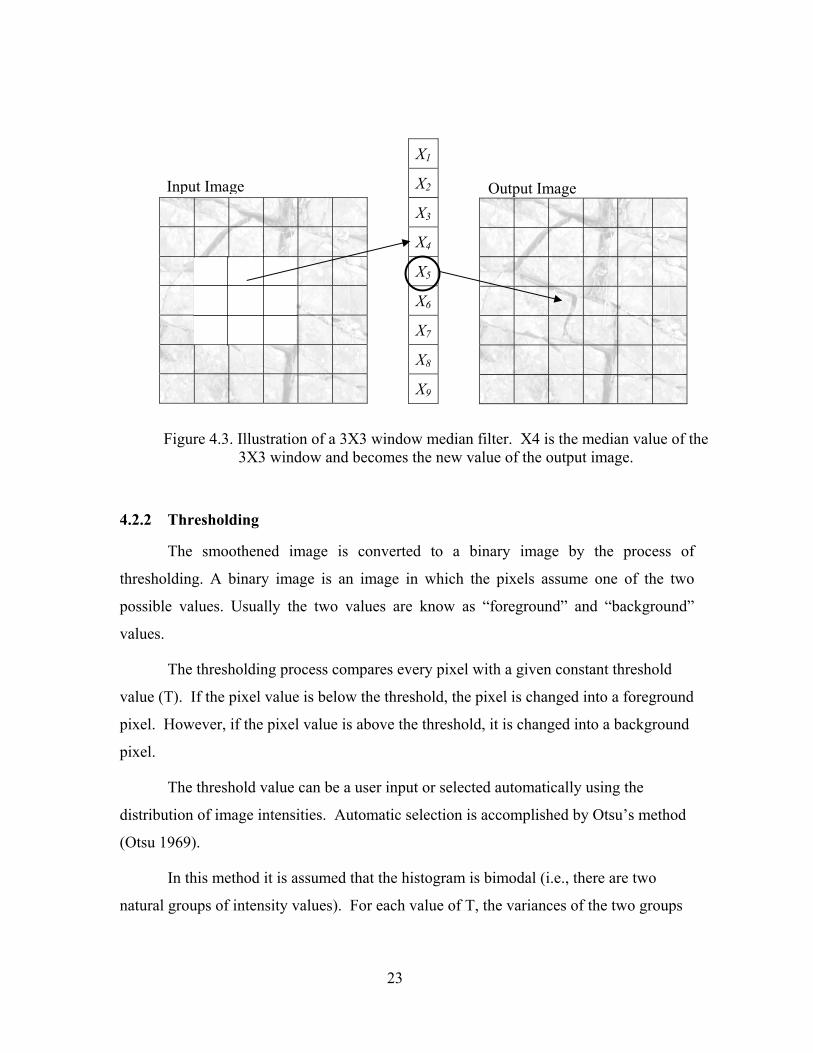
To implement a median smoothing filter, the user must first specify a window size
such as 3X3. Then, for each position of the window within the original image, the
algorithm sorts the pixel values in order then computes the statistical median of those
pixel values. This median value is the new pixel value on the output image. This process
is illustrated on Figure 4.3.
Page 32
23
4.2.2 Thresholding
The smoothened image is converted to a binary image by the process of
thresholding. A binary image is an image in which the pixels assume one of the two
possible values. Usually the two values are know as “foreground” and “background”
values.
The thresholding process compares every pixel with a given constant threshold
value (T). If the pixel value is below the threshold, the pixel is changed into a foreground
pixel. However, if the pixel value is above the threshold, it is changed into a background
pixel.
The threshold value can be a user input or selected automatically using the
distribution of image intensities. Automatic selection is accomplished by Otsu’s method
(Otsu 1969).
In this method it is assumed that the histogram is bimodal (i.e., there are two
natural groups of intensity values). For each value of T, the variances of the two groups
X1
X2
X3
X4
X5
X6
X7
X8
X9
Output Image
Input Image
Figure 4.3. Illustration of a 3X3 window median filter. X4 is the median value of the 3X3 window and becomes the new value of the output image.
Page 33
24
are computed. The threshold value is the value of T for which the expected value of the
group variance is minimum.
It can be mathematically expressed as follows:
q1 t( )= h i( ),i=0
t
∑ (4.2)
and
q2 t( )= h i( )i= t+1
255
∑ . (4.3)
The group variance, σ2 (t), is written as:
σw2 t( )= q1 t( )σ1
2 t( )+ q2 t( )σ 22 t( ). (4.4)
4.2.3 Thinning Thinning is used to obtain the fracture traces on the rock surface. Two thinning
algorithms are included in the program and the user can opt for either. The first thinning
algorithm is a sequential raster scanning algorithm also known as Hilditch algorithm,
Hilditch (1969). The second method is a parallel algorithm developed by Zhang and Suen
(1984). Each method is discussed below.
4.2.3.1 Hilditch’s Algorithm The Hilditch algorithm determines pixels for deletion from the image. Deletion in
this case means transferring from an object pixel to background pixel based on the
specified conditions described below. The algorithm traverses the image in a raster
scanning sequence from top to bottom and left to right. After each raster scan the
identified object points are transferred into background pixels. The algorithm stops when
no pixels are found that fulfills the criteria.
A pixel is removed if it satisfies all of the following conditions:
Condition 1. It is a foreground pixel, where:
I(r,c) = 1. (4.5)
Condition 2. It is located on the boundary. This is satisfied if at least one of its
four neighbors belongs to the background or has been removed from the
Page 34
25
foreground pixels. A pixel is considered to be on the background at the end of the
iteration. Figure 4.4 shows four possible arrangements of pixels, where P is the
pixel currently being considered by the algorithm.
The numbering sequence of the pixels is shown in Figure 4.5. The algorithm in
this step computes the value of the function f1(p) = a1 + a3 + a5 + a7 . If the pixel value at
ni =1 (foreground), then ai = 0 , otherwise ai = 1 . If f1(p) ≥ 1 then the pixel P will be
changed to background (value = 0).
Condition 3. It is not at the end of a thin line. This requires that at least two of its
eight neighbors not belong to the background nor have been removed from the
foreground pixels. This is determined as follows:
f2 (p) = bii=1
8
∑ , where bi = 1 if I(r,c) = 1 and bi = 0 otherwise.
If f2 (p) ≥ 2 , then the pixel P will be changed to background. (4.7)
Condition 4. It is not an isolated point, (at least one of its eight neighbors is a
foreground pixel).
1
1 P 1
0
Figure 4.4. Four possible arrangements of pixels.
Figure 4.5. Numbering sequence of the neighborhood pixels.
n4 n3 n2
n5 P n1
n6 n7 n8
0
1 P 1
1
1
1 P 0
1
1
0 P 1
1
Page 35
26
f3(p) = bii=1
8
∑ ,
where bi = 1 if I(r,c) = 1 and bi = 0 otherwise, and
f3( p) ≥ 1. (4.8)
Condition 5. If the removal of a pixel does not alter connectivity of the
foreground pixels. The number of connected components in the eight neighbor region is
determined using the Hilditch’s crossing number. The Hilditch‘s crossing number of a
pixel is calculated by determining how many neighbors belong to the background (value
=0) and has either one of their next two neighbors in the eight-neighborhood region that
is a foreground pixel or have been removed.
f4 (p) = XH (p) = cii=1
4
∑ , where ci = 1 if f (n2i−1) = 0 and either f (n2i ) > 0
or f (n2i+1) > 0 , ci = 0 otherwise) and,
f5 (p) = 1. (4.9)
The calculation of Hilditch’s crossing number is further illustrated in the
following example shown in Figure 4.6.
In the above example, though both the cases have four foreground pixels, the
crossing number is a minimum for one and a maximum for the other. In the example on
0 1 0
1 p 1
0 1 0
1 0 1
0 p 0
1 0 1
(a) Crossing Number XH(P) = 0
(b) Crossing Number XH(P) = 4
Figure 4.6. Example of Hilditch’s crossing number calculation.
Page 36
27
the left, each of the four adjacent neighbors are black pixels. In the example on the right,
the four diagonal neighbors, n2, n4, n6 and n8,of the 8-neighbor region are black pixels.
4.2.3.2 Parallel Algorithm
The second thinning algorithm provided in this application is a parallel algorithm
by Zhang and Suen (1984). This algorithm removes identified pixels from the foreground
region except those points that belong to the skeleton. Each iteration consists of two sub-
iterations also referred to as 'sub-cycles'. The first sub-iteration identifies the pixels to be
removed that are located on the south-east boundary and the north-west corners. The
second sub-iteration identifies the pixels to be removed that are located on the north-west
boundary and the south-east corners. Both the sub-iterations are necessary to preserve the
connectivity of the original regions on its skeleton because identified points are
transferred in parallel. The thinning process terminates when no additional points are
identified for deletion by both sub-iterations.
First Sub-Iteration. Each pixel in the image is examined and is deleted if it
satisfies all of the following conditions:
Condition 1. The pixel belongs to the foreground region (pixel value = 1).
f1(p) = 1 (4.10)
Condition 2. It is a pixel identified for deletion but not an isolated point or the
end of a thin line. The number of 8-neighbors that belong to the foreground region, is
greater than or equals to two, and less than or equals to six.
f2 (p) = nii=1
8
∑ , where 2 ≤ f2 (p) ≤ 6 (4.11)
Condition 3. The number of white pixels located before a black pixel within its 8-
neighbor region being equal to one. The 8-neighbors are ordered in the following
sequence: n3, n2, n1, n8, n7, n6, n5 and n4.
Equation 4.11 is calculated by counting the number of transitions from a pixel on
the foreground region to a pixel on the background and vice versa when traversing its 8-
neighbors in anti-clockwise direction. It can only be an even integer, because transitions
Page 37
28
must occur in pairs. If there is a transition between two pixels, there must be another
transition associated with it. The valid crossing number in this case is 2.
f3(p) = XR (p) = ni+1 − nii=1
8
∑ , f3(p) = 2 . (4.12)
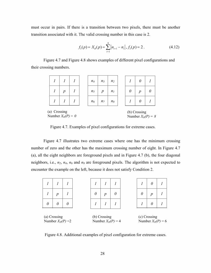
Figure 4.7 and Figure 4.8 shows examples of different pixel configurations and
their crossing numbers.
Figure 4.7 illustrates two extreme cases where one has the minimum crossing
number of zero and the other has the maximum crossing number of eight. In Figure 4.7
(a), all the eight neighbors are foreground pixels and in Figure 4.7 (b), the four diagonal
neighbors, i.e., n2, n4, n6 and n8 are foreground pixels. The algorithm is not expected to
encounter the example on the left, because it does not satisfy Condition 2.
n4 n3 n2
n5 p n1
n6 n7 n8
1 1 1
1 p 1
1 1 1
1 0 1
0 p 0
1 0 1
(a) Crossing Number XH(P) = 0
(b) Crossing Number XH(P) = 8
Figure 4.7. Examples of pixel configurations for extreme cases.
1 1 1
1 p 1
0 0 0
1 1 1
0 p 0
1 1 1
1 0 1
0 p 1
1 0 1
(a) Crossing Number XH(P) =2
(b) Crossing Number XH(P) = 4
(c) Crossing Number XH(P) = 6
Figure 4.8. Additional examples of pixel configuration for extreme cases.
Page 38
29
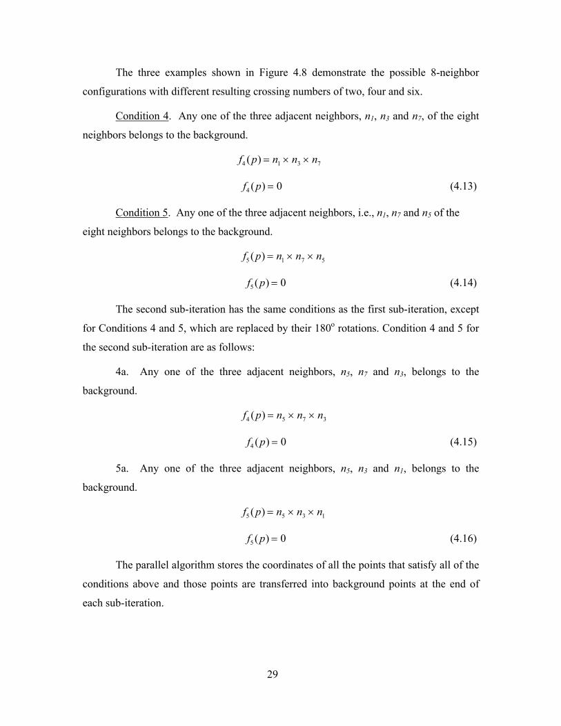
The three examples shown in Figure 4.8 demonstrate the possible 8-neighbor
configurations with different resulting crossing numbers of two, four and six.
Condition 4. Any one of the three adjacent neighbors, n1, n3 and n7, of the eight
neighbors belongs to the background.
f4 (p) = n1 × n3 × n7
f4 (p) = 0 (4.13)
Condition 5. Any one of the three adjacent neighbors, i.e., n1, n7 and n5 of the
eight neighbors belongs to the background.
f5 (p) = n1 × n7 × n5
f5 (p) = 0 (4.14)
The second sub-iteration has the same conditions as the first sub-iteration, except
for Conditions 4 and 5, which are replaced by their 180o rotations. Condition 4 and 5 for
the second sub-iteration are as follows:
4a. Any one of the three adjacent neighbors, n5, n7 and n3, belongs to the
background.
f4 (p) = n5 × n7 × n3
f4 (p) = 0 (4.15)
5a. Any one of the three adjacent neighbors, n5, n3 and n1, belongs to the
background.
f5 (p) = n5 × n3 × n1
f5 (p) = 0 (4.16)
The parallel algorithm stores the coordinates of all the points that satisfy all of the
conditions above and those points are transferred into background points at the end of
each sub-iteration.
Page 39
30
4.2.4 Fracture Separation
After the fracture trace map is extracted, the individual fracture traces are
separated and are saved as different image files. The starting point and the ending point
of the individual traces are determined by the following conditions.
1. Let P be the first foreground pixel encountered while performing raster scan.
2. If a node or junction is encountered then it is assumed that the endpoint of the
fracture is reached. Few examples of a node are shown in Figure 4.9. A pixel is identified
as a node if it has more than one foreground pixel in the neighborhood region represented
by n1, n2, n6, n7 and n8 as shown in Figure 4.10.
3. If a pixel does not have any foreground neighbors in the region shown in Figure
4.10 then, that pixel is identified as the end of the fracture trace.
n2
p n1
n6 n7 n8
1 0 0 0 1
0 1 0 1 0
0 0 1 0 0
0 0 1 0 0
0 0 1 0 0
1 0 0 0 1
0 1 0 1 0
0 0 1 0 0
0 1 0 0 0
1 0 0 0 0
Node
Figure 4.9. Neighborhood pixels while identifying nodes.
Figure 4.10. Examples of nodes.
Page 40
31
4. If the endpoint of the fracture trace is reached then the scanned fracture trace is
saved as a separate image file. The fracture properties are calculated and saved in a text
file.
4.2.5 Fracture Properties
Fracture properties such as length, orientation, width and large-scale roughness
are determined from the individual fracture traces. Length is determined by summing the
number of connected pixels in a fracture trace image multiplied by the size of the pixel.
Pixel size is determined from the scale of the image. If the length of the fracture trace is
less than a predefined length then the fracture trace is ignored. This is done to remove
noise. Orientation is determined by the slope of a straight line connecting the start and
end pixels of the trace map.
The width of the fracture trace is determined by returning to the threshold image.
Width is the number of foreground pixels in a direction perpendicular to the fracture trace
multiplied by the size of the pixel. This is illustrated in Figure 4.11.
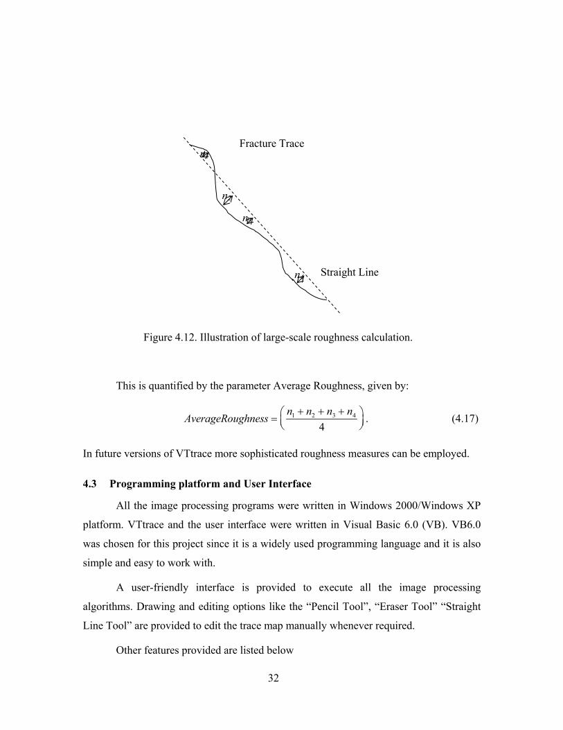
Large-scale average roughness is computed using a straight line connecting the
two end point pixels of the trace map (baseline). The perpendicular distance from the
baseline to the fracture trace is determined at random points. The average of all the
distances is a measure of large scale average roughness. This is illustrated in Figure 4.12.
Fracture trace from thresholded image
Direction of the trace
Direction in which width is determined
Figure 4.11. Direction in which the trace width is determined.
Page 41
32
This is quantified by the parameter Average Roughness, given by:
AverageRoughness =n1 + n2 + n3 + n4
4
. (4.17)
In future versions of VTtrace more sophisticated roughness measures can be employed.
4.3 Programming platform and User Interface
All the image processing programs were written in Windows 2000/Windows XP
platform. VTtrace and the user interface were written in Visual Basic 6.0 (VB). VB6.0
was chosen for this project since it is a widely used programming language and it is also
simple and easy to work with.
A user-friendly interface is provided to execute all the image processing
algorithms. Drawing and editing options like the “Pencil Tool”, “Eraser Tool” “Straight
Line Tool” are provided to edit the trace map manually whenever required.
Other features provided are listed below
n3
n4
Fracture Trace
Straight Line
n1
n2
Figure 4.12. Illustration of large-scale roughness calculation.
Page 42
33
• Zoom in.
• Pan.
• Undo.
• Redo.
• Options to change the pencil/line thickness.
The user can select the original image file using the “open” option on the main
menu. The sequence of process to extract the trace map can be done using the options
provided in the main menu. Option to print the trace map or the image is also provided.
Screen captures of the interface and the intermediate stages are shown in Figures 4.13 –
Figure 4.17.
Figure 4.13 Screen capture of the user interface.
Page 43
34
Figure 4.14. Screen Capture of the User Interface with a test image open.
Page 44
35
Figure 4.15. Screen Capture of the User Interface with a test image after
smoothing.
Page 45
36
Figure 4.16 Screen Capture of the User Interface with a test image after
thresholding.
Page 46
37
Figure 4.17 Screen Capture of the User Interface with a test image after thinning.
Page 47
38
Chapter 5 Test Cases and Results
This chapter presents results of a series of tests conducted to evaluate each image
processing algorithm and the performance of VTtrace as a whole. Each image processing
algorithm was tested with both synthetic images, prepared surfaces and natural rock
images. Synthetic images consisting of black lines on a white background were created
using the commercial program Adobe Illustrator. Images were also made of styrofoam
block discontinuity models consisting of black, hand-drawn lines on white background.
Images of natural surfaces were taken in local quarries and road cuts under daylight
conditions.
The user input for each stage of the individual image processing steps was varied
and the corresponding results are documented. After testing the individual algorithms, the
entire sequence of algorithms was executed with a set of test cases. This was done to
assess usability, process cycle length and resolve any algorithm integration issues.
For ease of reading, each of the following sections is written as stand-alone
discussions of each algorithm. Description of the test methodology particular to the
algorithm being tested, test results and interpretation of the results are presented in each
section. A critical discussion of the test results and each algorithm highlighting practical,
implementation issues is included.
5.1 Image Smoothing Algorithm
Smoothing is a process to reduce the noise or distortion in the image. Various
smoothing operators are available and were explained in Chapter 3. This section
describes the test cases used and results of the test sequence.
5.1.1 Methodology
A 3X3 median smoothing filter (Section 4.2.1) was implemented in VTtrace since
it is effective in enhancing edges and reducing noise with the least computational time.
The smoothing algorithm was tested with images of rock surfaces taken in ambient,
natural light conditions. The original image and the results after every pass of smoothing
are presented in Figures 5.1 to Figure 5.6. Artificial “salt and pepper” noise was
produced on some images and was tested for noise reduction using the smoothing
Page 48
39
program. The images with artificial salt-pepper noise and the results are shown in Figure
5.7 to Figure 5.8.
The criteria used for evaluating the effectiveness of the algorithm include the
distribution of the pixel intensity on the image and the sharpness of the edges forming the
fractures.
5.1.2 Results
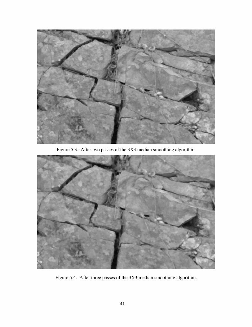
The results of the smoothing algorithm indicate its ability to reduce noise in the
image. It can be observed from the results that the smoothing operator makes the rock
surface more even and the edges are more prominent when compared to the original
image. By blending the values of the matrix pixels, it will be shown in the next section
that thresholding is simplified. The test on the image with the artificial salt and pepper
noise illustrates the capability of the algorithm to remove distortion and dead pixels.
5.1.3 Discussion
Practical issues with the smoothing operation include preservation of small
features, number of passes of the filter required, and the ability to automate the process.
One problem with the smoothing operation is that some thin or small features could be
lost, especially after multiple passes of the filter. Other practical problems are that the
number of passes of smoothing required and the window size (e.g., 3X3 or 5X5 or 7X7)
depends on the original image. The user is required to iterate using various combinations
of window size and choose whichever suits that particular image best.
At this time, it is not possible to fully automate this process for images of natural
surfaces in ambient light conditions. However where images are made in artificial light
conditions, it may be possible to impose some degree of smoothing by controlling the
intensity and type of lighting.
Page 49
40
Figure 5.1. Original image made in natural light conditions. Note the regions with lichen growth resulting in tonal differences.
Figure 5.2. After a single pass of the 3X3 median smoothing algorithm.
Page 50
41
Figure 5.3. After two passes of the 3X3 median smoothing algorithm.
Figure 5.4. After three passes of the 3X3 median smoothing algorithm.
Page 51
42
Figure 5.5. After four passes of the 3X3 median smoothing algorithm.
Figure 5.6. After five passes of the 3X3 median smoothing algorithm.
Page 52
43
Figure 5.7. Image with artificial “Salt and Pepper” noise.
Figure 5.8. Smoothed image with the “Salt and Pepper” noise removed.
Page 53
44
5.2 Thresholding Algorithm
Thresholding is the process of converting the grayscale image to a binary (black
and white) image. Due to the intensity difference between the pixels which form the
fracture trace and the pixels that form the rest of the rock surface, the fractures appear as
thick black lines. These lines form the basis of the fracture trace. The images are
smoothened before thresholding to reduce undesired noise.
5.2.1 Methodology
For testing the performance of this algorithm, the images were converted into
binary images after various levels of smoothing using different threshold values.
Threshold values ranged from 150 to 50. The algorithm was also tested on images
without smoothing for comparison.
5.2.2 Results
The results are presented in Figure 5.9 to Figure 5.19. It can be noticed in the
results that a high threshold value picks up any small intensity difference on the surface
and the width of the fracture is over represented. Low threshold value results in the
breaking fractures and width of the fracture is under represented. Selecting a correct
threshold value is crucial since it the basis of the fracture map and also the width of the
fractures are measure from the binary image.
5.2.3 Discussion
A high threshold value will result in some undesired spots on the binary image on
the other hand a low threshold value may result in some breaks on the fracture. The level
on smoothing also plays an important role in this process since smoothing alters the
intensity distribution in the image.
Practical problems for thresholding rock mass images include closely spaced
features, noise, and lighting irregularities. If the width of the fracture is small, the
thresholding operation will not detect that fracture. Also, if the fracture spacing is very
close, groups of fractures may be detected as a single feature. Although at the outset this
may seem a problem, it might prove to be a natural way for homogenizing the rock mass
into a numerically more tractable problem.
Page 54
45
Vegetation on the rock surfaces will require an additional step in processing to
remove. However for freshly excavated faces and for underground environments,
vegetation will not generally be present.
Figure 5.9. Binary image with threshold value of 150 after single pass 3X3 median
smoothing.
Page 55
46
Figure 5.10. Binary image with threshold value of 128 after single pass 3X3 median
smoothing.
Figure 5.11. Binary image with threshold value of 100 after single pass 3X3 median
smoothing.
Page 56
47
Figure 5.12 Binary image with threshold value of 75 after single pass 3X3 median
smoothing.
Figure 5.13 Binary image with threshold value of 50 after single pass of a 3X3 median
smoothing.
Page 57
48
Figure 5.14 Binary image with threshold value of 128 after five pass 3X3 median
smoothing.
Figure 5.15 Binary image with threshold value of 100 after five pass 3X3 median
smoothing.
Page 58
49
Figure 5.16. Binary image with threshold value of 150 without smoothing.
Figure 5.17. Binary image with threshold value of 128 without smoothing.
Page 59
50
Figure 5.18. Binary image with threshold value of 100 without smoothing.
Figure 5.19. Binary image with threshold value of 50 without smoothing.
Page 60
51
5.3 Thinning Algorithm
The binary image is thinned to extract the fracture trace map of the rock mass
exposure. The outcome of the thinning process is a network of lines that are a single pixel
in thickness which represent the fracture trace map.
5.3.1 Methodology
Two thinning algorithms namely the Hilditch’s algorithm (Stefanelli et al., 1971)
and the Zhang & Suen thinning method (Zhang et al. 1984) are provided. The user has
the option to select any of the algorithms for a particular image.
Both the thinning algorithms were tested with the images after different levels of
thresholding and smoothing. The effects of smoothing and thresholding can be clearly
visible on the thinned image. The results of the thinning algorithm are presented from
Figure 5.20 to Figure 5.31.
5.3.2 Results The result of the thinning algorithm shows that there are some basic differences
between the fracture trace maps produced by both the algorithms. Hilditch’s algorithm is
simple, fast and produces trace map of exactly one pixel thickness. Erosion of line
segments at the end points is more severe than the Zhang & Suen algorithm. If the image
has some isolated horizontal fractures, Hilditch’s algorithm cannot be used since it erodes
these features to a single pixel.
Objects such as a horizontal line, vertical line and a grid were created using
Adobe Illustrator and were thinned using both the algorithms. The results are compared
in Figures 5.32 to 5.34. The thinned images where edited using the editing options
provided in the program and the final fracture trace maps are shown in Figure 5.35.
5.3.3 Discussion The result of the thinning algorithm largely depends on the smoothing and
thresholding processes since there are no user input parameters for this process. The user
has the choice only to select one of the two algorithms for thinning. The results of the
thinning algorithm on the images with high threshold value generates a cluster of
Page 61
52
unwanted lines whereas the images with low threshold values generated broken traces.
Hence, thresholding is the critical process that determines the quality of the trace map.
Figure 5.20. Thinned image using Hilditch’s algorithm after single pass 3X3 smoothing
and threshold of 150.
Page 62
53
Figure 5.21. Thinned image using Hilditch’s algorithm after single pass 3X3 smoothing
and threshold of 128.
Figure 5.22. Thinned image using Hilditch’s algorithm after single pass 3X3 smoothing
and threshold of 100.
Page 63
54
Figure 5.23. Thinned image using Hilditch’s algorithm after single pass 3X3 smoothing
and threshold of 50.
Figure 5.24. Thinned image using Zhang & Suen algorithm after single pass 3X3
smoothing and threshold of 150.
Page 64
55
Figure 5.25. Thinned image using Zhang & Suen algorithm after single pass 3X3
smoothing and threshold of 128.
Page 65
56
Figure 5.26. Thinned image using Zhang & Suen algorithm after single pass 3X3
smoothing and threshold of 100.
Figure 5.27. Thinned image using Zhang & Suen algorithm after single pass 3X3
smoothing and threshold of 50.
Page 66
57
Figure 5.28. Thinned image using Hilditch’s algorithm after threshold of 120 without
smoothing.
Figure 5.29. Thinned image using Hilditch’s algorithm after threshold of 100 without
smoothing.
Page 67
58
Figure 5.30. Thinned image using Zhang & Suen algorithm after threshold of 128 without
smoothing.
Figure 5.31. Thinned image using Zhang & Suen algorithm after threshold of 100
without smoothing.
Page 68
59
(b)
(a)
(c)
Figure 5.32. Synthetic horizontal line and results of thinning by Zhang & Suen and
Hilditch’s algorithms: (a) Original synthetic image, (b) original image, Zhang &Suen
algorithm, (c) original image, Hilditch algorithm.
Page 69
60
(a) (b) (c)
Figure 5.33. Synthetic vertical line and results of thinning by Zhang & Suen and
Hilditch’s algorithms: (a) Original synthetic image, (b) Zhang & Suen algorithm, (c)
Hilditch algorithm.
Page 70
61
(a)
(b) (c)
Figure 5.34 Synthetic grid pattern and results of thinning by Zhang & Suen and
Hilditch’s algorithms: (a) Original synthetic image, (b) Zhang & Suen algorithm,
(c) Hilditch algorithm.
Page 71
62
Figure 5.35. Thinned image using Zhang & Suen algorithm after single pass 3X3
smoothing and threshold at 100 after manual editing using the editing tools.
Page 72
63
5.4 Feature characterization algorithm
The individual features are separated and stored as individual image files. The
feature attributes are determined from the separated features. The final trace map after
thinning and manual editing is used to obtain the feature properties such as trace length,
orientation, width and large-scale roughness. Synthetic images were tested and the results
are presented in Figure 5.36.
Page 73
64
Feature Properties: Length = 174 mm Orientation = 39 degrees Width = 2mm (c) Feature 1
Feature Properties: Length = 197 mm Orientation = 42 degrees Width = 2mm (d) Feature 2
(b) Thinned test image (a) Original test image before thinning
Page 74
65
Figure 5.36. Original synthetic image and result of the feature characterization algorithm.
Feature Properties: Length = 72 mm Orientation = -41.1805 degrees Width = 2mm (e). Feature 3
Feature Properties: Length = 186 mm Orientation = 41.1147 degrees Width = 2mm (f) Feature 4
Feature Properties: Length = 57 mm Orientation = -40.975 degrees Width = 2mm (g) Feature 5
Feature Properties: Length = 50 mm Orientation = -41.1339 degrees Width = 2mm (h). Feature 6
Feature Properties: Length = 59 mm Orientation = -41 degrees Width = 2mm (i) Feature 7
Page 75
66
5.5 Integration Testing
The complete sequence of stages was tested with test images of rock surfaces to
assess the program VTtrace as a whole.
5.5.1 Methodology To test the complete sequence of stages, an original image of a rock surface was
taken and all the algorithms were executed in sequence. Optimum parameters for each
algorithm were used as determined from the trials. For thinning, Zhang & Suen’s
algorithm was used since it gave better results than Hilditch’s algorithm. Total time taken
for the entire process and the ease of use were evaluated.
5.5.2 Results The total time taken to complete the entire sequence of steps was about 5 minutes.
The thinned image was edited manually to obtain the final trace map. The time taken for
manual editing is controlled by the thresholding operation since the binary image is the
basis for the thinning operation. In this case, a threshold value of 100 was selected and
the thinned image required less manual editing. The result of each stage is shown from
Figures 5.38 to 5.42. Some of the individual fractures with their properties are shown in
Figure 5.43.
5.5.3 Discussion VTtrace is an efficient way to extract the fracture trace map. However, there are
some practical problems associated with this approach that will need to be addressed in
future research. Lighting plays an important role in the accuracy of the trace map since
this approach utilizes the variation of light intensity levels at each pixel in the image.
The image processing cannot be fully automated at this time because human intervention
is required for selecting the required parameters at each stage of the process. For
example, the smoothing and thresholding process are trial and error based and the user
performs these operations iteratively and selects the parameter that results in the 'best'
image. The parameters for the two process varies for different images depending on
factors like lighting, surface texture and color, presence of vegetation and other
Page 76
67
interferences etc. The user should also make a choice of the thinning algorithm based on
which gives better results for a particular image.
Figure 5.37. Original image.
Page 77
68
Figure 5.38. Results of single pass 3X3 median smoothing filter.
Figure 5.39. Smoothed binary image at threshold value of 100.
Page 78
69
Figure 5.40. Result of the Zhang & Suen thinning method.
Figure 5.41. Final fracture trace map after some manual editing.
Page 79
70
Figure 5.42. Individual features with their associated properties.
Feature Properties: Length 65mm Orientation 17 degrees Width 3mm Roughness 3mm
Feature Properties: Length 26mm Orientation -59 degrees Width Roughness 2mm
Feature Properties: Length 12mm Orientation 20 degrees Width 2mm Roughness 2mm
Feature Properties: Length 55 mm Orientation – 86 degrees Width 4mm Roughness 2mm
Page 80
71
Chapter 6 Conclusions and Recommendations
VTtrace is an effective tool to aid in the solution of traditional problems in rock
mechanics. The system developed as a part of this research will require some
enhancement and optimization. Though the advantages of using such a system are quite
obvious, it is concluded that some practical challenges remain, as listed below.
1. Lighting plays a crucial role in the accuracy of this approach. High illumination
will wash out important features and low illumination will critically influence
thresholding and thinning which will also lead to the loss of important
information. If the system is used for underground excavations like tunneling
lighting can be controlled but for outcrops the amount of sunlight and the time
of the day must be considered.
2. Presence of shadows on the images can be a problem especially when the
images are taken at an inclined angle, the shadows of edges tend to make the
fractures thicker on the images.
3. The smoothing and thresholding operations require more than one trial with
different parameters to get satisfactory results. The number of iterations
required depends on the quality of image, texture and color of the rock surface,
illumination, etc.
4. Erosion of the lines during thinning process may lead to the underestimation of
the trace length.
5. Manual editing of the thinned image can be time consuming and laborious if
large number of complex images are used.
6.1 Recommendations for Future Enhancements
Enhancements and additional features aimed at improving the efficiency and
capabilities of the system are listed below.
1. Fully implement photogrammetry to obtain the feature properties in 3D space
such as true trace length, width and roughness. Currently these parameters are
determined in 2D image plane.
2. Optimization of the thinning algorithm to improve speed.
Page 81
72
3. Implementation of stereo matching techniques to extract the 3D coordinates of
key points on the features. This will be further used to develop the 3D model
of the rock mass.
4. Converting the individual fracture traces into vector objects so that the user
could pick a particular fracture trace and edit it. Currently raster editing is
implemented which appears to be more time consuming than vector editing in
many situations common to fracture mapping.
5. Implementation of an identification tool so that the user can pick a fracture
trace and the fracture properties would be displayed.
6. Migration to VB.Net since it has better image handling capabilities that VB 6.
7. Implement procedures and algorithms for tiling and georeferencing of images
for large rock exposures.
8. Creation of a database to store the fracture properties, images and any relevant
information.
9. Incorporate algorithm to obtain the dip and dip direction of the fractures.
10. Implement procedures and algorithms to identify and group joint sets.
With the implementation of the above additional features and the integration of
VTtrace into the AMADEUS system a significant contribution can be made in rock
mechanics. Other image processing techniques like edge detection and Hough transform
are some of the possible alternate solutions that might be incorporated in VTtrace. This
work has significantly improved our ability to detect discontinuity traces on rock surfaces
and will serve as a starting point for further research.
Page 82
73
Chapter 7 References Forsyth. A. D and Ponce, J. (2003). “Computer Vision A Modern Approach” Prentice
Hall Inc, New Jersey; United States of America.
Gaich, A., Fasching, A., and Gruber, M. (1999). “High Resolution Stereoscopic Imaging
for Tunnel Construction.” Rock and Soil Engineering Nr. 1/1999.
Gaich, A., Fasching, A., and Gruber, M. (http://www.ifb.tugraz.at/situ/). “Simulation in
Tunneling.” Research project report.
Jain, A. K. (1989). “Fundamentals of Digital Image Processing” Prentice Hall Inc, New
Jersey; United States of America.
Kemeny, J., Mofya, E., and Handy, J. (2003). “The use of Digital Imaging and laser
technologies for field rock Fracture Characterization.” Pan Am Conf 2003.
Klette, G. (2003). “A Comparative Discussion of Distance Transforms and Simple
Deformations in Digital Image Processing.” Project Report; University of Auckland;
Auckland; New Zealand.
Lemy, F., and Hadjigeorgiou, J., (2003). “Rock Mass Characterization Using Image
Analysis.” Pan Am Conf 2003.
Lewis, R. (1990). “Practical Digital Image Processing.” 1st Ed., Ellis Horwood Ltd., West
Sussex, England.
Soole, P. and Poropat, G. (2000). “SIRO 3D – A 3D Imaging for Geology &
Geotechnical Assessment.” report for CSIRO Exploration and Mining.
Pitas, I. (2000). “Digital Image Processing Algorithms and Applications.” 2nd Ed.,
Prentice Hall International, Great Britain.
Pratt, W. K. (2001). “Digital Image Processing” 3rd Ed., John Wiley & Sons, Inc.; United
States of America.
Reid, T.R. (1998). “Methodology for the detection of discontinuity traces in digital
images of rock mass exposures.” PhD thesis, University of London, London,
England.
Reid, T.R., and Harrison J.P., (2000). “A semi-automated methodology for discontinuity
trace detection in digital images of rock mass exposures.” International journal of
rock Mechanics and Mining Sciences 37 (2000) 1073-1089.
Page 83
74
Stefanelli, R and Rosenfeld, A. (1971). “Some Parallel Thinning Algorithms for Digital
Pictures.” Journal of the Association for Computing Machinery, Vol. 18, No. 2, April
1971, pp. 255-264.
Zhang, T. Y., and C. Y. Suen, C. Y. (1984). “A fast thinning algorithm for thinning
digital patterns.” Communications of the ACM; Vol. 27; Number 3; March 1984.