Munich Personal RePEc Archive A non-cooperative Pareto-efficient solution to a one-shot Prisoner’s Dilemma Wu, Haoyang 5 April 2011 Online at https://mpra.ub.uni-muenchen.de/34953/ MPRA Paper No. 34953, posted 24 Nov 2011 17:00 UTC
Transcript
Munich Personal RePEc Archive
A non-cooperative Pareto-efficient
solution to a one-shot Prisoner’s
Dilemma
Wu, Haoyang
5 April 2011
Online at https://mpra.ub.uni-muenchen.de/34953/
MPRA Paper No. 34953, posted 24 Nov 2011 17:00 UTC
A non-cooperative Pareto-efficient solution to
the one-shot Prisoner’s Dilemma
Haoyang Wu ∗
Abstract
The Prisoner’s Dilemma is a simple model that captures the essential contradictionbetween individual rationality and global rationality. Although the one-shot Pris-oner’s Dilemma is usually viewed simple, in this paper we will categorize it intofive different types. For the type-4 Prisoner’s Dilemma game, we will propose a self-enforcing algorithmic model to help non-cooperative agents obtain Pareto-efficientpayoffs. The algorithmic model is based on an algorithm using complex numbersand can work in macro applications.
The Prisoner’s Dilemma (PD) is perhaps the most famous model in the fieldof game theory. Roughly speaking, there are two sorts of PD: one-shot PD anditerated PD. Nowadays a lot of studies on PD are focused on the latter case.For example, Axelrod [1] investigated the evolution of cooperative behavior inwell-mixed populations of selfish agents by using PD as a paradigm. Nowakand May [2] induced spatial structure in PD, i.e., agents were restricted tointeract with his immediate neighbors. Santos and Pacheco [3] found that whenagents interacted following scale-free networks, cooperation would become adominating trait throughout the entire range of parameters of PD. Perc andSzolnoki [4] proposed that social diversity could induce cooperation as thedominating trait throughout the entire range of parameters of PD.
∗ Wan-Dou-Miao Research Lab, Suite 1002, 790 WuYi Road, Shanghai, 200051,China.
Compared with the iterated PD, the one-shot PD is usually viewed simple. Inthe original version of one-shot PD, two prisoners are arrested by a policeman.Each prisoner must independently choose a strategy between “Confessing”(denoted as strategy “Defect”) and “Not confessing” (denoted as strategy“Cooperate”). The payoff matrix of prisoners is shown in Table 1. As long astwo agents are rational, the unique Nash equilibrium shall be (Defect, Defect),which results in a Pareto-inefficient payoff (P, P ). That is the dilemma.
Table 1: The payoff matrix of PD, where T > R > P > S, and R > (T +S)/2.The first entry in the parenthesis denotes the payoff of agent 1 and the secondentry stands for the payoff of agent 2.XXXXXXXXXXXXagent 1
agent 2Cooperate Defect
Cooperate (R, R) (S, T)
Defect (T, S) (P, P)
In 1999, Eisert et al [5] proposed a quantum model of one-shot PD (denoted asEWL model). The EWL model showed “quantum advantages” as a result of anovel quantum Nash equilibrium, which help agents reach the Pareto-efficientpayoff (R,R). Hence, the agents escape the dilemma. In 2002, Du et al [6]gave an experiment to carry out the EWL model.
So far, there are some criticisms on EWL model: 1) It is a new game whichhas new rules and thus has no implications on the original one-shot PD [7]. 2)The quantum state serves as a binding contract which let the players choosesone of the two possible moves (Cooperate or Defect) of the original game. 3)In the full three-parameter strategy space, there is no such quantum Nashequilibrium [8] [9].
Besides these criticisms, here we add another criticism: in the EWL model,the arbitrator is required to perform quantum measurements to readout themessages of agents. This requirement is unreasonable for common macro dis-ciplines such as politics and economics, because the arbitrator should play aneutral role in the game: His reasonable actions should only receive agents’strategies and assign payoffs to agents. Put differently, if the arbitrator iswilling to work with an additional quantum equipment which helps agents toobtain the Pareto-efficient payoffs (R,R), then why does not he directly assignthe Pareto-efficient payoffs to the agents?
Motivated by these criticisms, this paper aims to investigate whether a Pareto-efficient outcome can be reached by non-cooperative agents in macro applica-tions. Note that a non-cooperative game is one in which players make decisionsindependently. Thus, while they may be able to cooperate, any cooperationmust be self-enforcing [10].
2
The rest of this paper is organized as follows: in Section 2 we will proposean algorithmic model, where the arbitrator does not have to work with someadditional quantum equipment (Note: here we do not aim to solve the firstthree criticisms on the EWL model, because these criticisms are irrelevant tothe algorithmic model). In Section 3, we will categorize the one-shot PD intofive different types, and claim that the agents can self-enforcingly reach thePareto-efficient outcome for the case of type-4 PD by using the algorithmicmodel. The Section 4 gives some discussions. The last section draws conclusion.
2 An algorithmic model
As we have pointed out above, for macro applications, it is unreasonable torequire the arbitrator act with some additional quantum equipment. In whatfollows, firstly we will amend the EWL model such that the arbitrator worksin the same way as he does in classical environments, then we will propose analgorithmic version of the amended EWL model.
2.1 The amended EWL model
Let the set of two agents be N = 1, 2. Following formula (4) in Ref. [9],two-parameter quantum strategies are drawn from the set:
(where γ is an entanglement measure, σx is the Pauli matrix, ⊗ is tensorproduct), I ≡ ω(0, 0), D ≡ ω(π, π/2), C ≡ ω(0, π/2).
Without loss of generality, we assume:1) Each agent j ∈ N has a quantum coin (qubit), a classical card and a chan-nel connected to the arbitrator. The basis vectors |C〉 = [1, 0]T , |D〉 = [0, 1]T
of a quantum coin denote head up and tail up respectively.2) Each agent j ∈ N independently performs a local unitary operation onhis/her own quantum coin. The set of agent j’s operation is Ωj = Ω. A
strategic operation chosen by agent j is denoted as ωj ∈ Ωj. If ωj = I, then
ωj(|C〉) = |C〉, ωj(|D〉) = |D〉; If ωj = D, then ωj(|C〉) = |D〉, ωj(|D〉) = |C〉.I denotes “Not flip”, D denotes “Flip”.3) The two sides of a card are denoted as Side 0 and Side 1. The messages writ-ten on the Side 0 (or Side 1) of card j is denoted as card(j, 0) (or card(j, 1)).
3
ψ
ψ
+
ω
ω
!
! " #
$
ψ %ψ
card(j, 0) represents “Cooperate”, and card(j, 1) represents “Defect”.4) There is a device that can measure the state of two quantum coins andsend messages to the designer.
Fig. 1 shows the amended version of EWL model (denoted as the A-EWLmodel). Its working steps are defined as follows:Step 1: The state of each quantum coin is set as |C〉. The initial state of thetwo quantum coins is |ψ0〉 = |CC〉.Step 2: Let the two quantum coins be entangled by J . |ψ1〉 = J |CC〉.Step 3: Each agent j independently performs a local unitary operation ωj on
his own quantum coin. |ψ2〉 = [ω1 ⊗ ω2]J |CC〉.Step 4: Let the two quantum coins be disentangled by J+. |ψ3〉 = J+[ω1 ⊗ω2]J |CC〉.Step 5: The device measures the state of the two quantum coins and sendscard(j, 0) (or card(j, 1)) as the message mj to the arbitrator if the collapsedstate of quantum coin j is |C〉 (or |D〉).Step 8: The arbitrator receives the overall message m = (m1,m2) and assignspayoffs to the two agents according to Table 1. END.
In the A-EWL model, the assumed device performs quantum measurementsand sends messages to the arbitrator on behalf of agents. Thus, the arbitra-tor needs not work with an additional quantum equipment as EWL modelrequires, i.e., the arbitrator works in the same way as before. It should be em-phasized that the A-EWL model does not aim to solve the criticisms on theEWL model as specified in the Introduction. We propose the A-EWL modelonly for the following simulation process, which is a key part of the algorithmicmodel.
Since quantum operations can be simulated classically by using complex num-bers, the A-EWL model can also be simulated. In what follows we will givematrix representations of quantum states and then propose an algorithmicversion of A-EWL model.
4
2.2 Matrix representations of quantum states
In quantum mechanics, a quantum state can be described as a vector. For atwo-level system, there are two basis vectors: [1, 0]T and [0, 1]T . In the begin-ning, we define:
Since only two values in ψ1 are non-zero, we only need to calculate the leftmostand rightmost column of ω1 ⊗ ω2 to derive ψ2 = [ω1 ⊗ ω2]ψ1.
Definition 2: ψ3 ≡ J+ψ2.
Suppose ψ3 = [η1, · · · , η4]T , let ∆ = [|η1|2, · · · , |η4|2]. It can be easily checked
that J , ω1, ω2 and J+ are all unitary matrices. Hence, |ψ3|2 = 1. Thus, ∆ canbe viewed as a probability distribution over the states |CC〉, |CD〉, |DC〉, |DD〉.
5
φξ
φξ
2.3 An algorithmic model
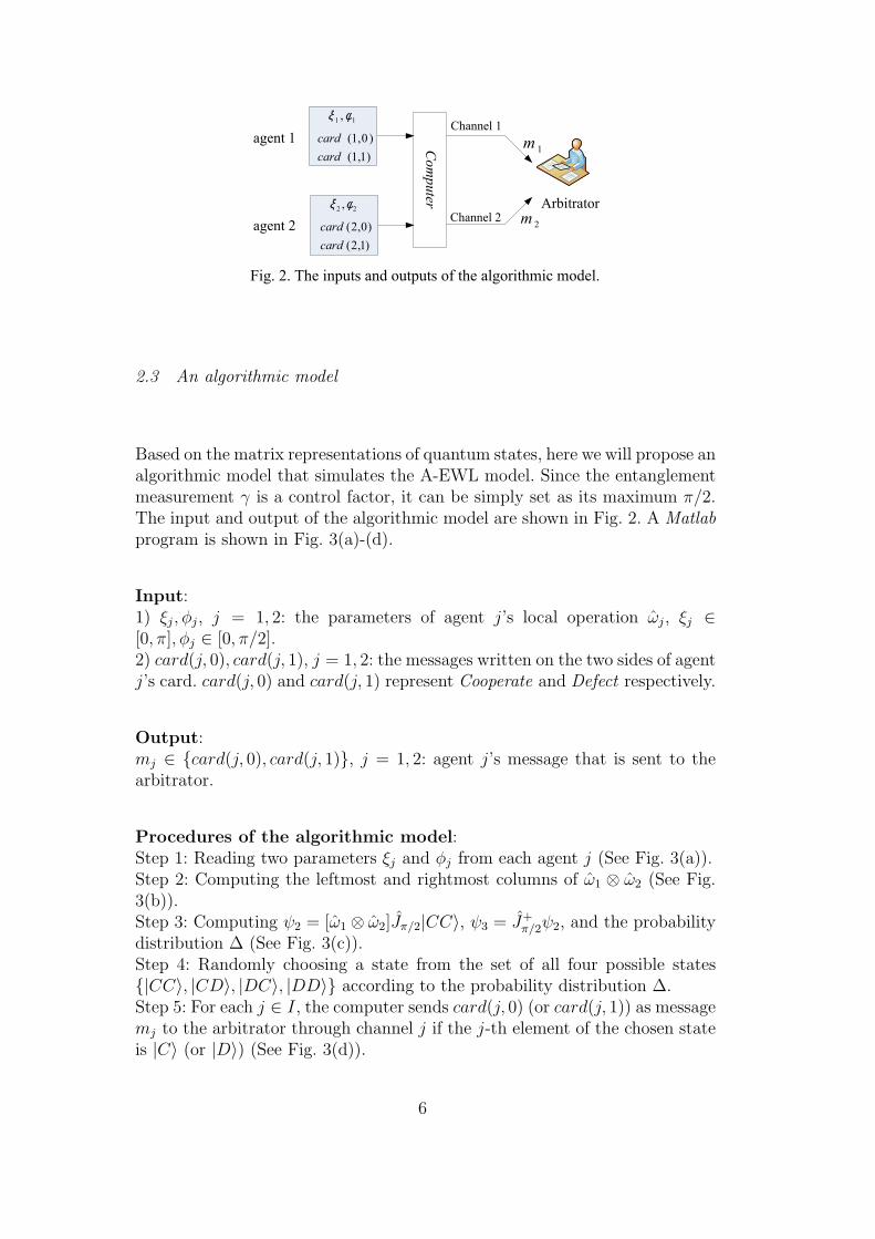
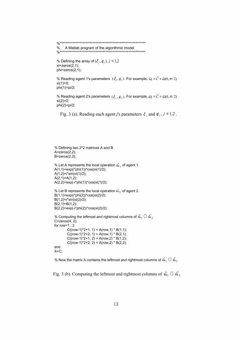
Based on the matrix representations of quantum states, here we will propose analgorithmic model that simulates the A-EWL model. Since the entanglementmeasurement γ is a control factor, it can be simply set as its maximum π/2.The input and output of the algorithmic model are shown in Fig. 2. A Matlabprogram is shown in Fig. 3(a)-(d).
Input:1) ξj, φj, j = 1, 2: the parameters of agent j’s local operation ωj, ξj ∈[0, π], φj ∈ [0, π/2].2) card(j, 0), card(j, 1), j = 1, 2: the messages written on the two sides of agentj’s card. card(j, 0) and card(j, 1) represent Cooperate and Defect respectively.
Output:mj ∈ card(j, 0), card(j, 1), j = 1, 2: agent j’s message that is sent to thearbitrator.
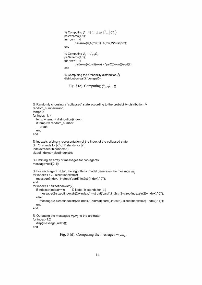
Procedures of the algorithmic model:Step 1: Reading two parameters ξj and φj from each agent j (See Fig. 3(a)).Step 2: Computing the leftmost and rightmost columns of ω1 ⊗ ω2 (See Fig.3(b)).Step 3: Computing ψ2 = [ω1 ⊗ ω2]Jπ/2|CC〉, ψ3 = J+
π/2ψ2, and the probability
distribution ∆ (See Fig. 3(c)).Step 4: Randomly choosing a state from the set of all four possible states|CC〉, |CD〉, |DC〉, |DD〉 according to the probability distribution ∆.Step 5: For each j ∈ I, the computer sends card(j, 0) (or card(j, 1)) as messagemj to the arbitrator through channel j if the j-th element of the chosen stateis |C〉 (or |D〉) (See Fig. 3(d)).
6
3 Five types of one-shot PD
Since its beginning, PD has been generalized to many disciplines such as pol-itics, economics, sociology, biology and so on. Despite these widespread ap-plications, people seldom care how the payoffs of agents are determined. Forexample, Axelrod [1] used the word “yield” to describe how the agents ob-tained the payoffs. Nowak and May [2] used the word “get”, and Santos andPacheco [3] used the word “receive” respectively.
One may think that such question looks trivial at first sight. However, as wewill show in this section, there exists an interesting story behind this question.In what follows, we will categorize the one-shot PD into five different types.
Type-1 PD:1) There are two agents and no arbitrator in the game.2) The strategies of agents are actions performed by agents. The agents’ payoffsare determined by the outcomes of these actions and satisfy Table 1.
For example, let us neglect the United Nation and consider two countries (e.g.,US and Russia) confronted the problem of nuclear disarmament. The strat-egy Cooperate means “Obeying disarmament”, and Defect means “Refusingdisarmament”. If the payoff matrix confronted by the two countries satisfiesTable 1, the nuclear disarmament game is a type-1 PD.
Type-2 PD:1) There are two agents and an arbitrator in the game.2) The strategies of agents are actions performed by agents. The arbitratorobserves the outcomes of actions and assign payoffs to the agents accordingto Table 1.
For example, let us consider a taxi game. Suppose there are two taxi driversand a manager. Two drivers drive a car in turn, one in day and the other innight. The car’s status will be very good, ok or common if the number of driverswho maintain the car is two, one or zero respectively. The manager observesthe car’s status and assigns rewards R2, R1, R0 to each driver respectively,where R2 > R1 > R0. The whole cost of maintenance is c. Let the strategyCooperate denote “Maintain”, and Defect denote “Not maintain”. The payoffmatrix can be represented as Table 2. If Table 2 satisfies the conditions inTable 1, the taxi game is a type-2 PD.
Table 2: The payoff matrix of type-2 PD.
7
XXXXXXXXXXXXagent 1agent 2
Cooperate Defect
Cooperate (R2 − c/2, R2 − c/2) (R1 − c, R1)
Defect (R1, R1 − c) (R0, R0)
Type-3 PD:1) There are two agents and an arbitrator in the game.2) The strategy of each agent is not an action, but a message that can be sentto the arbitrator through a channel. The arbitrator receives two messages andassign payoffs to the agents according to Table 1.3) Two agents cannot communicate with each other.
For example, suppose two agents are arrested separately and required to reporttheir crime information to the arbitrator through two channels independently.If the arbitrator assigns payoffs to agents according to Table 1, this game is atype-3 PD.
Type-4 PD:Conditions 1-2 are the same as those in type-3 PD.3) Two agents can communicate with each other.4) Before sending messages to the arbitrator, two agents can construct thealgorithmic model specified in Fig. 2. Each agent j can observe whether theother agent participates the algorithmic model or not: whenever the otheragent takes back his channel, agent j will do so and sends his message mj tothe arbitrator directly.
Remark 1 : At first sight, the conditions of type-4 PD is complicated. How-ever, these conditions are not restrictive when the arbitrator communicatewith agents indirectly and cannot separate them. For example, suppose thearbitrator and agents are connected by Internet, then all conditions of type-4PD can be satisfied in principle.
The type-4 PD works in the following way:Stage 1: (Actions of two agents) For each agent j ∈ N , he faces two strategies:• S(j, 0): Participate the algorithmic model, i.e., leave his channel to the com-puter, and submit ξj, φj, card(j, 0), card(j, 1) to the computer;• S(j, 1): Not participate the algorithmic model, i.e., take back his channel,and submit mj to the arbitrator directly.According to condition 4, the algorithmic model is triggered if and only if bothtwo agents participate it.Stage 2: (Actions of the arbitrator) The arbitrator receives two messages andassigns payoffs to agents according to Table 1.
In type-4 PD, from the viewpoints of the arbitrator, he acts in the same wayas before, i.e., nothing is changed. However, the payoff matrix confronted by
8
two agents is now changed to Table 3. For each entry of Table 3, we give thecorresponding explanation as follows:
Table 3: The payoff matrix of two agents by constructing the algorithmic model,where R,P are defined in Table 1, R > P .XXXXXXXXXXXXagent 1
agent 2S(2, 0) S(2, 1)
S(1, 0) (R, R) (P, P)
S(1, 1) (P, P) (P, P)
1) (S(1, 0), S(2, 0)): This strategy profile means two agents both participatethe algorithmic model and submit parameters to the computer. Accordingto Ref. [5], for each agent j ∈ N , his dominant parameters are ξj = 0 andφj = π/2, which result in a Pareto-efficient payoff (R,R).2) (S(1, 0), S(2, 1)): This strategy profile means agent 1 participates the algo-rithmic model, but agent 2 takes back his channel and submits a message tothe arbitrator directly. Since agent 1 can observe agent 2’s action, in the end,both agents will take back their channels and submit messages to the arbi-trator directly. Obviously, the dominant message of each agent j is card(j, 1),and the arbitrator will assign the Pareto-inefficient payoff (P, P ) to agents.3) (S(1, 1), S(2, 0)): This strategy profile is similar to the above case. The ar-bitrator will assign (P, P ) to two agents.4) (S(1, 1), S(2, 1)): This strategy profile means two agents both take backtheir channels and send messages to the arbitrator directly. This case is simi-lar to the case 2. The arbitrator will assign (P, P ) to two agents.
From Table 3, it can be seen that (S(1, 0), S(2, 0)) and (S(1, 1), S(2, 1)) are twoNash equilibria, and the former is Pareto-efficient. As specified by Telser (Page28, Line 2, [11]), “A party to a self-enforcing agreement calculates whether hisgain from violating the agreement is greater or less than the loss of future netbenefits that he would incur as a result of detection of his violation and the con-sequent termination of the agreement by the other party.” Since two channelshave been controlled by the computer in Stage 1, in the end (S(1, 0), S(2, 0))is a self-enforcing Nash equilibrium and the Pareto-efficient payoff (R,R) isthe unique Nash equilibrium outcome. In this sense, the two agents escape thedilemma.
Type-5 PD:Conditions 1-3 are the same as those in type-4 PD.4) The last condition of type-4 PD does not hold.For this case, although the two agents can communicate before moving andagree that collaboration is good for each agent, they will definitely choose(Defect, Defect) as if they are separated. Thus, the agents cannot escape thedilemma.
9
4 Discussions
The algorithmic model revises common understanding on the one-shot PD.Here we will discuss some possible doubts about it.
Q1 : The type-4 PD seems to be a cooperative game because in condition 4,the algorithmic model constructed by two agents acts as a correlation betweenagents.
A1 : From the viewpoints of agents, the game is different from the originalone-shot PD, since the payoff matrix confronted by the two agents has beenchanged from Table 1 to Table 3. But from the viewpoints of the arbitra-tor, nothing is changed. Thus, the so-called correlation between two agents isindeed unobservable to the arbitrator. Put differently, the arbitrator cannotprevent agents from constructing the algorithmic model.On the other hand, since each agent can freely choose not to participate thealgorithmic model and send a message to the arbitrator directly in Stage 1,the algorithmic model is self-enforcing and thus still a non-cooperative game.
Q2 : After the algorithmic model is triggered, can it simply send (card(1, 0),card(2, 0)) to the arbitrator instead of running Steps 1-5?
A2 : The algorithmic model enlarges each agent’s strategy space from the orig-inal strategy space Cooperate, Defect to a two-dimensional strategy space[0, π]× [0, π/2], and generates the Pareto-efficient payoff (R,R) in Nash equi-librium. The enlarged strategy space includes the original strategy space ofone-shot PD: the strategy (Cooperate, Cooperate), (Cooperate, Defect), (De-fect, Cooperate), (Defect, Defect) in the original PD correspond to the strategy((0, 0), (0, 0)), ((0, 0), (π, π/2)), ((π, π/2), (0, 0)), ((π, π/2), (π, π/2)) in the al-gorithmic model respectively, since I = ω(0, 0), D = ω(π, π/2).However, the idea in this question restricts each agent’s strategy space fromthe original strategy space Cooperate, Defect to a single strategy Cooperate.In this sense, two agents are required to sign a binding contract to do so. Thisis beyond the range of non-cooperative game.
Remark 2 : The algorithmic model is not suitable for type-1 and type-2 PD,because the computer cannot perform actions on behalf of agents. The algo-rithmic model is not applicable for type-3 PD either because two agents areseparated, thereby the algorithmic model cannot be constructed. For the caseof type-5 PD, the algorithmic model is not applicable because condition 4 intype-4 PD is vital and indispensable.
10
5 Conclusion
In this paper, we categorize the well-known one-shot PD into five types andpropose an algorithmic model to help two non-cooperative agents self-enforcinglyescape a special type of PD, i.e., the type-4 PD. The type-4 PD is justifiedwhen the arbitrator communicate with the agents indirectly through somechannels, and each agent’s strategy is not an action, but a message that canbe sent to the arbitrator. With the rapid development of Internet, more andmore type-4 PD games will be seen.
One point is important for the novel result: Usually people may think the twopayoff matrices confronted by agents and the arbitrator are the same (i.e.,Table 1). However we argue that for the case of type-4 PD, the two payoffmatrices can be different: The arbitrator still faces Table 1, but the agentscan self-enforcingly change their payoff matrix to Table 3 by virtue of thealgorithmic model, which leads to a Pareto-efficient payoff.
Acknowledgments
The author is very grateful to Ms. Fang Chen, Hanyue Wu (Apple), HanxingWu (Lily) and Hanchen Wu (Cindy) for their great support.
References
[1] R. Axelrod, W.D. Hamilton, The evolution of cooperation, Science, 211 (1981)1390-1396.
[2] M.A. Nowak, R.M. May, Evolutionary games and spatial chaos, Nature, 359(1992) 826-829.
[3] F.C. Santos, J.M. Pacheco, Scale-free networks provide a unifying frameworkfor the emergence of cooperation, Phys. Rev. Lett., 95 (2005) 098104.
[4] M. Perc and A. Szolnoki, Social diversity and promotion of cooperation in thespatial prisoner’s dilemma game, Phys. Rev. E, 77 (2008) 011904.
[5] J. Eisert, M. Wilkens, M. Lewenstein, Quantum games and quantum strategies,Phys. Rev. Lett., 83 (1999) 3077-3080.
[6] J. Du, H. Li, X. Xu, M. Shi, J. Wu, X. Zhou and R. Han, Experimentalrealization of quantum games on a quantum computer, Phys. Rev. Lett., 88(2002) 137902.
11
[7] S. J. van Enk and R. Pike, Classical rules in quantum games, Phys. Rev. A 66
(2002) 024306.
[8] S.C. Benjamin, P.M. Hayden, Comment on “Quantum Games and QuantumStrategies”, Phys. Rev. Lett. 87 (2001) 069801.
[9] A.P. Flitney and L.C.L. Hollenberg, Nash equilibria in quantum games withgeneralized two-parameter strategies, Phys. Lett. A 363 (2007) 381-388.
[10] http://en.wikipedia.org/wiki/Non-cooperative game
[11] L.G. Telser, A theory of self-enforcing agreements. Journal of Business 53
(1980) 27-44.
12
%************************************************************% A Matlab program of the algorithmic model%************************************************************
% Defining the array of xi=zeros(2,1);phi=zeros(2,1);
% Reading agent 1's parameters . For example,xi(1)=0;phi(1)=pi/2;
% Reading agent 2's parameters . For example, xi(2)=0;phi(2)=pi/2;
πωω ==
πωω ==
= φξ
φξ
φξ
ξ =φ
% Defining two 2*2 matrices A and BA=zeros(2,2);B=zeros(2,2);
% Let A represents the local operation of agent 1.A(1,1)=exp(i*phi(1))*cos(xi(1)/2);A(1,2)=i*sin(xi(1)/2);A(2,1)=A(1,2);A(2,2)=exp(-i*phi(1))*cos(xi(1)/2);
% Let B represents the local operation of agent 2.B(1,1)=exp(i*phi(2))*cos(xi(2)/2);B(1,2)=i*sin(xi(2)/2);B(2,1)=B(1,2);B(2,2)=exp(-i*phi(2))*cos(xi(2)/2);
% Computing the leftmost and rightmost columns of C=zeros(4, 2);for row=1 : 2
% indexstr: a binary representation of the index of the collapsed state% ‘0’ stands for , ‘1’ stands for indexstr=dec2bin(index-1);sizeofindexstr=size(indexstr);
% Defining an array of messages for two agentsmessage=cell(2,1);
% For each agent , the algorithmic model generates the messagefor index=1 : 2 - sizeofindexstr(2) messageindex,1=strcat('card(',int2str(index),',0)');endfor index=1 : sizeofindexstr(2) if indexstr(index)=='0' % Note: ‘0’ stands for message2-sizeofindexstr(2)+index,1=strcat('card(',int2str(2-sizeofindexstr(2)+index),',0)');