A Non-homogeneous Time Mixed Integer LP Formulation...

A Non-homogeneous Time Mixed Integer LPFormulation for Traffic Signal Control

Iain GuilliardNational ICT Australia7 London CircuitCanberra, ACT, [email protected]

Scott SannerOregon State University1148 Kelley Engineering CenterCorvallis, OR [email protected]

Felipe W. TrevizanNational ICT Australia7 London CircuitCanberra, ACT, [email protected]

Brian C. WilliamsMassachusetts Institute of Technology77 Massachusetts AvenueCambridge, MA [email protected]

5258 words + 8 figures + 0 table + 27 citations(Weighted total words: 7258 out of 7000 + 35 references)March 17, 2016

ABSTRACTAs urban traffic congestion is on the increase worldwide, it is critical to maximize capacity andthroughput of existing road infrastructure through optimized traffic signal control. To this end, webuild on the body of work in mixed integer linear programming (MILP) approaches that attempt tojointly optimize traffic signal control over an entire traffic network and specifically on improvingthe scalability of these methods for large numbers of intersections. Our primary insight in this workstems from the fact that MILP-based approaches to traffic control used in a receding horizon con-trol manner (that replan at fixed time intervals) need to compute high fidelity control policies onlyfor the early stages of the signal plan; therefore, coarser time steps can be employed to “see” overa long horizon to preemptively adapt to distant platoons and other predicted long-term changesin traffic flows. To this end, we contribute the queue transmission model (QTM) which blendselements of cell-based and link-based modeling approaches to enable a non-homogeneous timeMILP formulation of traffic signal control. We then experiment with this novel QTM-based MILPcontrol in a range of traffic networks and demonstrate that the non-homogeneous MILP formula-tion achieves (i) substantially lower delay solutions, (ii) improved per-vehicle delay distributions,and (iii) more optimal travel times over a longer horizon in comparison to the homogeneous MILPformulation with the same number of binary and continuous variables.

Guilliard, Sanner, Trevizan, and Williams 2

INTRODUCTIONAs urban traffic congestion is on the increase worldwide with estimated productivity losses in thehundreds of billions of dollars in the U.S. alone and immeasurable environmental impact (1), it iscritical to maximize capacity and throughput of existing road infrastructure through optimized traf-fic signal control. Unfortunately, many large cities still use some degree of fixed-time control (2)even if they also use actuated or adaptive control methods such as SCATS (3) or SCOOT (4).However, there is further opportunity to improve traffic signal control even beyond adaptive meth-ods through the use of optimized controllers (that incorporate elements of both adaptive and actu-ated control) as evidenced in a variety of approaches including mixed integer (linear) program-ming (5, 6, 7, 8, 9, 10), heuristic search (11, 12), queuing delay with pressure control (13) andlinear program control (14), to scheduling-driven control (15, 16), and reinforcement learning (2).Such optimized controllers hold the promise of maximizing existing infrastructure capacity byfinding more complex (and potentially closer to optimal) jointly coordinated intersection policiesin comparison to heuristically-adaptive policies such as SCATS and SCOOT. However, optimizedmethods are computationally demanding and often do not guarantee jointly optimal solutions overa large intersection network either because (a) they only consider coordination of neighboring in-tersections or arterial routes or (b) they fail to scale to large intersection networks simply for com-putational reasons. We remark that the latter scalability issue is endemic to many mixed integerprogramming approaches to optimized signal control.

In this work, we build on the body of work in mixed integer linear programming (MILP) ap-proaches that attempt to jointly optimize traffic signal control over an entire traffic network (ratherthan focus on arterial routes) and specifically on improving the scalability of these methods forlarge urban traffic networks. In our investigation of existing approaches in this vein, namely exem-plar methods in the spirit of (7, 9) that use a (modified) cell transmission model (CTM) (17, 18) fortheir underlying prediction of traffic flows, we remark that a major drawback is the CTM-imposedrequirement to choose a predetermined homogeneous (and often necessarily small) time step forreasonable modeling fidelity. This need to model a large number of CTM cells with a small timestep leads to MILPs that are exceedingly large and often intractable to solve.

Our primary insight in this work stems from the fact that MILP-based approaches to trafficcontrol used in a receding horizon control manner (that replan at fixed time intervals) need tocompute high fidelity control policies only for the early stages of the signal plan; therefore, coarsertime steps can be employed to “see” over a long horizon to preemptively adapt to distant platoonsand other predicted long-term changes in traffic flows. This need for non-homogeneous control inturn spawns the need for an additional innovation: we require a traffic flow model that permits non-homogeneous time steps and properly models the travel time delay between lights. To this end,we might consider CTM extensions such as the variable cell length CTM (19), stochastic CTM(20, 21), CTM extensions for better modeling freeway-urban interactions (22) including CTMhybrids with link-based models (23), assymmetric CTMs for better handling flow imbalances inmerging roads (24), the situational CTM for better modeling of boundary conditions (25), andthe lagged CTM for improved modeling of the flow density relation (26). However, despite thewidespread varieties of the CTM and usage for a range of applications (27), there seems to be noextension that permits non-homogeneous time steps as proposed in our novel MILP-based controlapproach.

For this reason, as a major contribution of this work to enable our non-homogeneoustime MILP-based model of joint intersection control, we contribute the queue transmission model


(a)

q1

q7

q9

pl6

: EW NS

t :

NS

n : 51 32 4 6 7 8

5.30.0 2.01.0 4.1 5.8 6.5 8.8

t : 0.51.0 2.11.0 1.2 0.7 2.3

dl6,EW

: 4.30.0 1.0 2.10.0 3.1 4.3 4.3 4.3

dl6,NS

: 0.00.0 1.0 1.01.0 1.0 0.5 1.2 3.5

0

max

0

0

max

EW EW EW NS NS NS

(b)

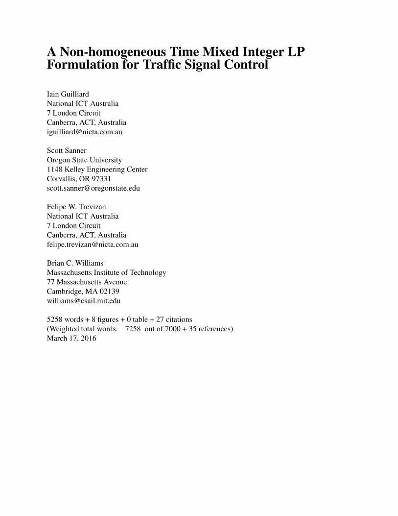
FIGURE 1 (a) Example of a real traffic network modeled using the QTM. (b) A previewof different QTM model parameters as a function of non-homogeneous discretized time in-tervals indexed by n. For each n, we show the following parameters: the elapsed time t,the non-homogeneous time step length �t, the cumulative duration d of two different lightphases for l

6

, the phase p of light l6

, and the traffic volume of different queues q linearly in-terpolated between time points. There is technically a binary p for each phase, but we abusenotation and simply show the current active phase: NS for north-south green and EW foreast-west green assuming the top of the map is north. Here we see that traffic progresses fromq1

to q7

to q9

according to light phases and traffic propagation delay with non-homogeneoustime steps only at required changepoints. We refer to the QTM model section for precisenotation and technical definitions.

(QTM) that blends elements of cell-based and link-based modeling approaches as illustrated andsummarized in Figure 1. The QTM offers the following key benefits:

• Unlike previous CTM-based joint intersection signal optimization (7, 9), the QTM isintended for non-homogeneous time steps that can be used for control over large horizons.

• Any length of roadway without merges or diverges can be modeled as a single queueleading to compact QTM MILP encodings of large traffic networks (i.e., large numbers ofcells and their associated MILP variables are not required between intersections). Further,the free flow travel time of a link can be modeled exactly, independent of the discritizaitontime step, while CTM requires a further increased discretization to approach the sameresolution.

• The QTM accurately models fixed travel time delays critical to green wave coordinationas in (5, 6, 8) through the use of a non-first order Markovian update model and furthercombines this with fully joint intersection signal optimization in the spirit of (7, 9, 10).

In the remainder of this paper, we first formalize our novel QTM model of traffic flowwith non-homogeneous time steps and show how to encode it as a linear program for computingtraffic flows. Next we proceed to allow the traffic signals to become discrete phase variables thatare optimized subject to a delay minimizing objective and standard minimum and maximum time


constraints for cycles and phases; this results in our final MILP formulation of traffic signal control.We then experiment with this novel QTM-based MILP control in a range of traffic networks anddemonstrate that the non-homogeneous MILP formulation achieves (i) substantially lower delaysolutions, (ii) improved per-vehicle delay distributions, and (iii) more optimal travel times over alonger horizon in comparison to the homogeneous MILP formulation with the same number ofbinary and continuous variables.

THE QUEUE TRANSMISSION MODEL (QTM)A Queue Transmission Model (QTM) is the tuple (Q,L, ~�t, I), where Q and L are, respectively,the set of queues and lights; ~

�t is a vector of size N representing the homogeneous, or non-homogeneous, discretization of the problem horizon [0,T] and the duration in seconds of the n-thtime interval is denoted as �t

n

; and I is a matrix |Q| ⇥ T in which I

i,n

represents the flow ofvehicles requesting to enter queue i from the outside of the network at time n.

A traffic light ` 2 L is defined as the tuple (

min

`

,

max

`

,P`

,

~

�

min

`

,

~

�

max

`

), where:

• P`

is the set of phases of `;

• min

`

( max

`

) is the minimum (maximum) allowed cycle time for `; and

• ~

�

min

`

(~�max

`

) is a vector of size |P`

| and �min

`,k

(�max

`,k

) is the minimum (maximum) allowedtime for phase k 2 P

`

.

A queue i 2 Q represents a segment of road that vehicles traverse at free flow speed; oncetraversed, the vehicles are vertically stacked in a stop line queue. Formally, a queue i is defined bythe tuple (Q

i

,T

prop

i

,F

out

i

,

~

F

i

,

~

Pr

i

,QPi

) where:

• Q

i

is the maximum capacity of i;

• T

prop

i

is the time required to traverse i and reach the stop line;

• F

out

i

represents the maximum traffic flow from i to the outside of the modeled network;

• ~

F

i

and ~

Pr

i

are vectors of size |Q| and their j-th entry (i.e., Fi,j

and Pr

i,j

) represent themaximum flow from queue i to j and the turn probability from i to j (where

Pj2Q Pr

i,j

=

1), respectively; and

• QPi

is the set of traffic light phases controlling the outflow of queue i, where the pair,(`, k) 2 QP

i

, denotes phase k of light `.

Differently than the CTM (9, 17), the QTM does not assume that�t

n

= T

prop

i

for all n, thatis, the QTM can represent non-homogeneous time intervals (Figure 1(b)). The only requirementover �t

n

is that no traffic light maximum phase time is smaller than any �t

n

since phase changesoccur only between time intervals; formally, �t

n

min

`2L,k2P`�

max

`,k

for all n 2 {1, . . . ,N}.


Computing Traffic Flows with QTMIn this section, we present how to compute traffic flows using QTM and non-homogeneous timeintervals �t. We assume for the remainder of this section that a valid control plan for all trafficlights is fixed and given as parameter; formally, for all ` 2 L, k 2 P

`

, and interval n 2 {1, . . . , N},the binary variable p

`,k,n

is known a priori and indicates if phase k of light ` is active (i.e., p`,k,n

=

1) or not on interval n. Each phase k 2 P`

can control the flow from more than one queue, allowingarbitrary intersection topologies to be modelled, including “all red” phases as a switching penaltyand modeling lost time from amber lights.

We represent the problem of finding the maximal flow between capacity-constrained queuesas a Linear Program (LP) over the following variables defined for all intervals n 2 {1, . . . ,N} andqueues i and j:

• q

i,n

2 [0,Q

i

]: traffic volume waiting in the stop line of queue i at the beginning ofinterval n;

• f

in

i,n

2 [0, I

i,n

]: inflow to the network via queue i during interval n;

• f

out

i,n

2 [0,F

out

i

]: outflow from the network via queue i during interval n; and

• f

i,j,n

2 [0,F

i,j

]: flow from queue i into queue j during interval n.

The maximum traffic flow from queue i to queue j is enforced by constraints (C1) and (C2).(C1) ensures that only the fraction Pr

i,j

of the total internal outflow of i goes to j, and since eachf

i,j,n

appears on both sides of (C1), the upstream queue i will block if any downstream queue j

is full. (C2) forces the flow from i to j to be zero if all phases controlling i are inactive (i.e.,p

`,k,n

= 0 for all (l, k) 2 QPi

). If more than one phase p

`,k,n

is active, then (C2) is subsumed bythe domain upper bound of f

i,j,n

.

f

i,j,n

Pr

i,j

|Q|X

k=1

f

i,k,n

(C1)

f

i,j,n

F

i,j

X

(l,k)2QPi

p

`,k,n

(C2)

To simplify the presentation of the remainder of the LP, we define the helper variablesq

in

i,n

(C3), qouti,n

(C4), and t

n

(C5) to represent the volume of traffic to enter and leave queue i duringinterval n, and the time elapsed since the beginning of the problem until the end of interval �t

n

,respectively.

q

in

i,n

= �t

n

(f

in

i,n

+

|Q|X

j=1

f

j,i,n

) (C3)

q

out

i,n

= �t

n

(f

out

i,n

+

|Q|X

j=1

f

i,j,n

) (C4)

t

n

=

nX

x=1

�t

x

(C5)


In order to account for the misalignment of the different �t and T

prop

i

, we need to find thevolume of traffic that entered queue i between two arbitrary points in time x and y (x 2 [0,T],y 2 [0,T], and x < y), i.e., x and y might not coincide with any t

n

for n 2 {1, . . . , N}. Thisvolume of traffic, denoted as V

i

(x, y), is obtained by integrating q

in

i,n

over [x, y] and is defined in (1)where m and w are the index of the time intervals s.t. t

m

x < t

m+1

and t

w

y < t

w+1

. Becausethe QTM dynamics are piecewise linear, qin

i,n

is a step function w.r.t. time and this integral reducesto the sum of qin

i,n

over the intervals contained in [x, y] and the appropriate fraction of qini,m

and q

in

i,w

representing the misaligned beginning and end of [x, y].

V

i

(x, y) = (t

m+1

� x)

q

in

i,m

�t

m

+

w�1X

k=m+1

q

in

i,k

!+ (y � t

w

)

q

in

i,w

�t

w

(1)

Using these helper variables, (C6) represents the flow conservation principle for queue i

where Vi

(t

n�1

�T

prop

i

, t

n

�T

prop

i

) is the volume of vehicles that reached the stop line during�t

n

.Since ~

�t and T

prop

i

for all queues are known a priori, the indexes m and w used by V

i

can be pre-computed in order to encode (1); moreover, (C6) represents a non-first order Markovian updatebecause the update considers the previous w � m time steps. To ensure that the total volume oftraffic traversing i (i.e., V

i

(t

n

�T

prop

i

, t

n

)) and waiting at the stop line does not exceed the capacityof the queue, we apply (C7). When queue i is full, qin

i,n

= 0 by (C7), which forces fj,i,n

to 0 in (C3)and (C4). This in turn allows the queue in i to spill back into the upstream queue j.

q

i,n

= q

i,n�1

� q

out

i,n�1

+ V

i

(t

n�1

� T

prop

i

, t

n

� T

prop

i

) (C6)V

i

(t

n

� T

prop

i

, t

n

) + q

i,n

Q

i

(C7)

As with MILP formulations of CTM (e.g. Lin and Wang (9)), QTM is also susceptible towithholding traffic, i.e., the optimizer might prevent vehicles from moving from i to j even thoughthe associated traffic phase is active and j is not full, e.g., this may reserve space for traffic froman alternate approach that allows the MILP to minimize delay in the long-term even though itleads to unintuitive traffic flow behavior. We address this well-known issue through our objectivefunction (O1) by maximizing the total outflow q

out

i,n

(i.e., both internal and external outflow) of iplus the inflow f

in

i,n

from the outside of the network to i. This quantity is weighted by the remainingtime until the end of the problem horizon T to force the optimizer to allow as much traffic volumeas possible into the network and move traffic to the outside of the network as soon as possible.

max

NX

n=1

|Q|X

i=1

(T� t

n

+ 1)(f

out

i,n

+ f

in

i,n

) (O1)

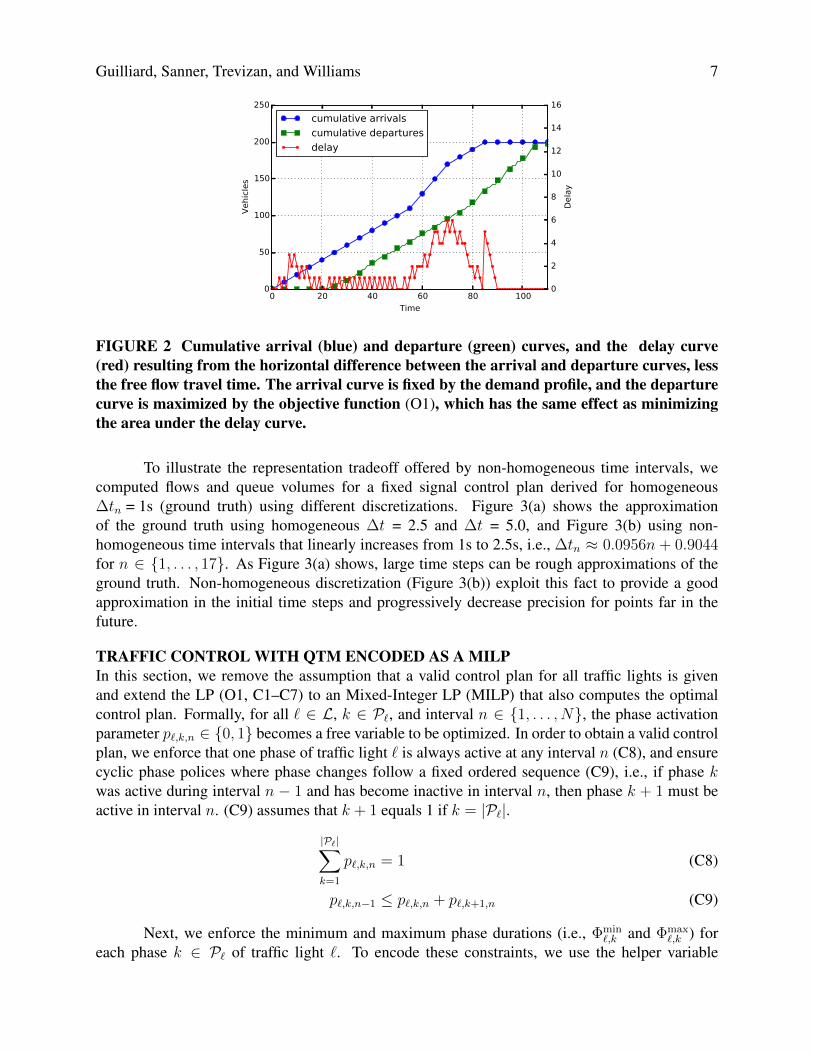
The objective (O1) corresponds to minimizing delay in CTM models, e.g., (O1) is equiva-lent to the objective function (O3) in Lin and Wang (9) for their parameters ↵ = 1, � = 1 for theorigin cells, and � = 0 for all other cells. Figure 2 depicts this equivalence using the cumulativenumber of vehicles entering and leaving a network as a function of time. The delay experienced bythe vehicles travelling through this network (red curve in Figure 2) equals the horizontal differenceat each point between the cumulative departure and arrival curves (less the free flow travel timethrough the network). Maximizing f

out

i,n

weighted by (T � t

n

+ 1) in (O1) is the same as forcingthe departure curve to be as close as possible to the arrival curve as early as possible; therefore, thearea between arrival and departure is minimized, which in turn minimizes the delay.


FIGURE 2 Cumulative arrival (blue) and departure (green) curves, and the delay curve(red) resulting from the horizontal difference between the arrival and departure curves, lessthe free flow travel time. The arrival curve is fixed by the demand profile, and the departurecurve is maximized by the objective function (O1), which has the same effect as minimizingthe area under the delay curve.

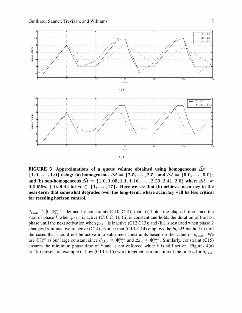
To illustrate the representation tradeoff offered by non-homogeneous time intervals, wecomputed flows and queue volumes for a fixed signal control plan derived for homogeneous�t

n

= 1s (ground truth) using different discretizations. Figure 3(a) shows the approximationof the ground truth using homogeneous �t = 2.5 and �t = 5.0, and Figure 3(b) using non-homogeneous time intervals that linearly increases from 1s to 2.5s, i.e., �t

n

⇡ 0.0956n + 0.9044

for n 2 {1, . . . , 17}. As Figure 3(a) shows, large time steps can be rough approximations of theground truth. Non-homogeneous discretization (Figure 3(b)) exploit this fact to provide a goodapproximation in the initial time steps and progressively decrease precision for points far in thefuture.

TRAFFIC CONTROL WITH QTM ENCODED AS A MILPIn this section, we remove the assumption that a valid control plan for all traffic lights is givenand extend the LP (O1, C1–C7) to an Mixed-Integer LP (MILP) that also computes the optimalcontrol plan. Formally, for all ` 2 L, k 2 P

`

, and interval n 2 {1, . . . , N}, the phase activationparameter p

`,k,n

2 {0, 1} becomes a free variable to be optimized. In order to obtain a valid controlplan, we enforce that one phase of traffic light ` is always active at any interval n (C8), and ensurecyclic phase polices where phase changes follow a fixed ordered sequence (C9), i.e., if phase k

was active during interval n � 1 and has become inactive in interval n, then phase k + 1 must beactive in interval n. (C9) assumes that k + 1 equals 1 if k = |P

`

|.

|P`|X

k=1

p

`,k,n

= 1 (C8)

p

`,k,n�1

p

`,k,n

+ p

`,k+1,n

(C9)

Next, we enforce the minimum and maximum phase durations (i.e., �min

`,k

and �max

`,k

) foreach phase k 2 P

`

of traffic light `. To encode these constraints, we use the helper variable


(a)

(b)

FIGURE 3 Approximations of a queue volume obtained using homogeneous ~�t ={1.0, . . . , 1.0} using: (a) homogeneous ~�t = {2.5, . . . , 2.5} and ~�t = {5.0, . . . , 5.0};and (b) non-homogeneous ~�t = {1.0, 1.05, 1.1, 1.16, . . . , 2.29, 2.41, 2.5} where�tn ⇡0.0956n + 0.9044 for n 2 {1, . . . , 17}. Here we see that (b) achieves accuracy in thenear-term that somewhat degrades over the long-term, where accuracy will be less criticalfor receding horizon control.

d

`,k,n

2 [0,�

max

`,k

], defined by constraints (C10–C14), that: (i) holds the elapsed time since thestart of phase k when p

`,k,n

is active (C10,C11); (ii) is constant and holds the duration of the lastphase until the next activation when p

`,k,n

is inactive (C12,C13); and (iii) is restarted when phase kchanges from inactive to active (C14). Notice that (C10–C14) employs the big-M method to turnthe cases that should not be active into subsumed constraints based on the value of p

`,k,n

. Weuse �max

`,k

as our large constant since d

`,k,n

�

max

`,k

and �t

n

�

max

`,k

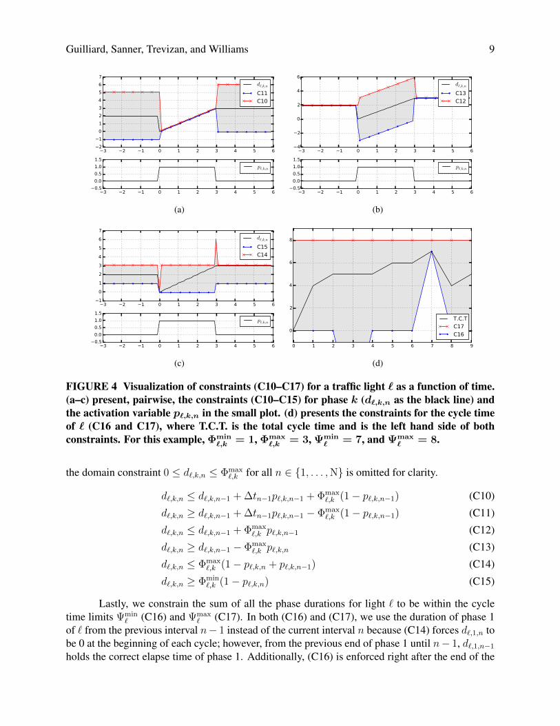
. Similarly, constraint (C15)ensures the minimum phase time of k and is not enforced while k is still active. Figures 4(a)to 4(c) present an example of how (C10–C15) work together as a function of the time n for d

`,k,n

;


(a) (b)

(c) (d)

FIGURE 4 Visualization of constraints (C10–C17) for a traffic light ` as a function of time.(a–c) present, pairwise, the constraints (C10–C15) for phase k (d`,k,n as the black line) andthe activation variable p`,k,n in the small plot. (d) presents the constraints for the cycle timeof ` (C16 and C17), where T.C.T. is the total cycle time and is the left hand side of bothconstraints. For this example, �min

`,k = 1, �max

`,k = 3, min

` = 7, and max

` = 8.

the domain constraint 0 d

`,k,n

�max

`,k

for all n 2 {1, . . . ,N} is omitted for clarity.

d

`,k,n

d

`,k,n�1

+�t

n�1

p

`,k,n�1

+ �

max

`,k

(1� p

`,k,n�1

) (C10)d

`,k,n

� d

`,k,n�1

+�t

n�1

p

`,k,n�1

� �max

`,k

(1� p

`,k,n�1

) (C11)d

`,k,n

d

`,k,n�1

+ �

max

`,k

p

`,k,n�1

(C12)d

`,k,n

� d

`,k,n�1

� �max

`,k

p

`,k,n

(C13)d

`,k,n

�max

`,k

(1� p

`,k,n

+ p

`,k,n�1

) (C14)d

`,k,n

� �min

`,k

(1� p

`,k,n

) (C15)

Lastly, we constrain the sum of all the phase durations for light ` to be within the cycletime limits min

`

(C16) and max

`

(C17). In both (C16) and (C17), we use the duration of phase 1of ` from the previous interval n� 1 instead of the current interval n because (C14) forces d

`,1,n

tobe 0 at the beginning of each cycle; however, from the previous end of phase 1 until n� 1, d

`,1,n�1

holds the correct elapse time of phase 1. Additionally, (C16) is enforced right after the end of the


each cycle, i.e., when its first phase is changed from inactive to active. The value (C16) and (C17)over time for a traffic light ` is illustrated in Figure 4(d).

d

`,1,n�1

+

|P`|X

k=2

d

`,k,n

� min

`

(p

`,1,n

� p

`,1,n�1

) (C16)

d

`,1,n�1

+

|P`|X

k=2

d

`,k,n

max

`

(C17)

The MILP that encodes the problem of finding the optimal traffic control plan in a QTM networkis defined by (O1, C1–C17).

EMPIRICAL EVALUATIONIn this section we compare the solutions for traffic networks modeled as a QTM using homo-geneous and non-homogeneous time intervals w.r.t. to two evaluation criteria: the quality of thesolution and convergence to the optimal solution vs. the number of time steps. Specifically, wecompare the quality of solutions based on the total travel time and we also consider the third quar-tile and maximum of the observed delay distribution. The hypotheses we wish to evaluate in thispaper are: (i) the quality of the non-homogeneous solutions is at least as good as the homoge-neous ones when the number of time intervals N is fixed; and (ii) the non-homogeneous approachrequires less time intervals (i.e., smaller N) than the homogeneous approach to converge to theoptimal solution. In the remainder of this section, we present the traffic networks considered in theexperiments, our methodology, and the results.

NetworksWe consider three networks of increasing complexity (Figure 5): an avenue crossed by three sidestreets; a 2-by-3 grid; and a 3-by-3 grid with a diagonal avenue. The queues receiving vehiclesfrom outside of the network are marked in Figure 5 and we refer to them as input queues. Themaximum queue capacity (Q

i

) is 60 vehicles for non-input queues and infinity for input queues toprevent interruption of the input demand due to spill back from the stop line. The traversal time ofeach queue i (Tprop

i

) is set at 9s (a distance of 125m with a free flow speed of 50km/h). For eachstreet, flows are defined from the head of each queue i into the tail of the next queue j; there is noturning traffic (Pr

i,j

= 1), and the maximum flow rate between queues, Fi,j

, is set at 5 vehicles/s.All traffic lights have two phases, north-south and east-west, and lights 2, 4 and 6 of network 3have the additional northeast-southwest phase to control the diagonal avenue. For networks 1 and2, �min

`,k

is 1s, �max

`,k

is 3s, min

`

is 2s, and max

`

is 6s, for all traffic light ` and phase k. For network3, �min

`,k

is 1s and �max

`,k

is 6s for all ` and k; and min

`

is 2s and max

`

is 12s for all lights ` exceptfor lights 2, 4 and 6 (i.e., lights also used by the diagonal avenue) in which min

`

is 3s and max

`

is18s.

Experimental MethodologyFor each network, a constant background level traffic is injected in the network in the first 55s toallow the solver to settle on a stable policy. Then a spike in demand is introduced in the queuesmarked as � (Figure 5) from time 55s to 70s to trigger a policy change. From time 70s to 85s,the demand is returned to the background level, and then reduced to zero for all input queues. We


(a) (b)

(c) (d)

FIGURE 5 (a–c) Networks used to evaluate the QTM performance. (d) Demand profile ofthe queues marked as }, |, and � for our experiments.

extend the problem horizon T until all vehicles have left the network. By clearing the network,we can easily measure the total travel time for all the traffic as the area between the cumulativearrival and departure curves measured at the boundaries of the network. The background levelfor the input queues are 1, 4 and 2 vehicles/s for queues marked as }, | and � (Figure 5(d)),respectively; and during the high demand period, the queues � receive 4 vehicles/s.

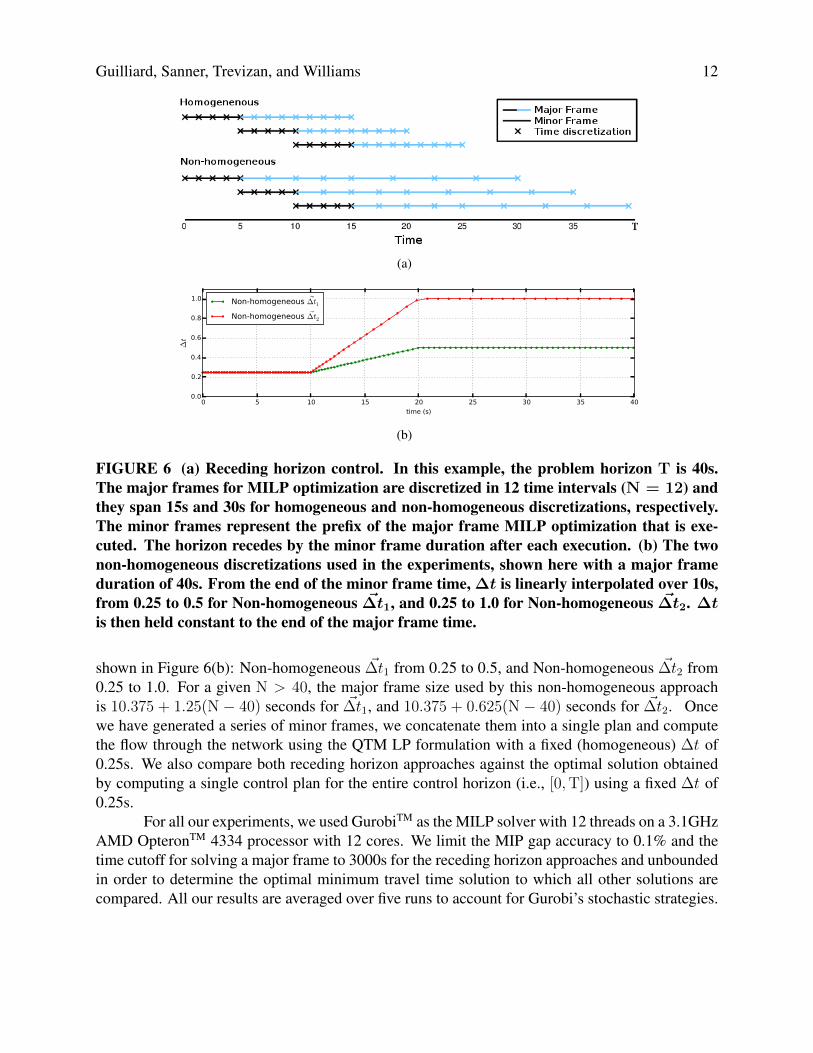
For both homogeneous and non-homogeneous intervals, we use the MILP QTM formula-tion in a receding horizon manner: a control plan is computed for a pre-defined horizon (smallerthan T) and only a prefix of this plan is executed before generating a new control plan. Figure 6(a)depicts our receding horizon approach and we refer to the planning horizon as a major frame andits executable prefix as a minor frame. Notice that, while the plan for a minor frame is beingexecuted, we can start computing the solution for the next major frame based on a forecast model.

To perform a fair comparison between the homogeneous and non-homogeneous discretiza-tions, we fix the size of all minor frames to 10s and force it to be discretized in homogeneousintervals of 0.25s. For the homogeneous experiments, �t is kept at 0.25s throughout the majorframe; therefore, given N, the major frame size equals N/4 seconds for the homogeneous ap-proach. For the non-homogeneous experiments, we increase�t linearly from the end of the minorframe for 10s and then hold it constant to the end of the major frame. We use two discretizations as


(a)

(b)

FIGURE 6 (a) Receding horizon control. In this example, the problem horizon T is 40s.The major frames for MILP optimization are discretized in 12 time intervals (N = 12) andthey span 15s and 30s for homogeneous and non-homogeneous discretizations, respectively.The minor frames represent the prefix of the major frame MILP optimization that is exe-cuted. The horizon recedes by the minor frame duration after each execution. (b) The twonon-homogeneous discretizations used in the experiments, shown here with a major frameduration of 40s. From the end of the minor frame time,�t is linearly interpolated over 10s,from 0.25 to 0.5 for Non-homogeneous ~�t

1

, and 0.25 to 1.0 for Non-homogeneous ~�t2

. �tis then held constant to the end of the major frame time.

shown in Figure 6(b): Non-homogeneous ~

�t

1

from 0.25 to 0.5, and Non-homogeneous ~

�t

2

from0.25 to 1.0. For a given N > 40, the major frame size used by this non-homogeneous approachis 10.375 + 1.25(N � 40) seconds for ~

�t

1

, and 10.375 + 0.625(N � 40) seconds for ~

�t

2

. Oncewe have generated a series of minor frames, we concatenate them into a single plan and computethe flow through the network using the QTM LP formulation with a fixed (homogeneous) �t of0.25s. We also compare both receding horizon approaches against the optimal solution obtainedby computing a single control plan for the entire control horizon (i.e., [0,T]) using a fixed �t of0.25s.

For all our experiments, we used GurobiTM as the MILP solver with 12 threads on a 3.1GHzAMD OpteronTM 4334 processor with 12 cores. We limit the MIP gap accuracy to 0.1% and thetime cutoff for solving a major frame to 3000s for the receding horizon approaches and unboundedin order to determine the optimal minimum travel time solution to which all other solutions arecompared. All our results are averaged over five runs to account for Gurobi’s stochastic strategies.


(a) (b)

(c) (d)

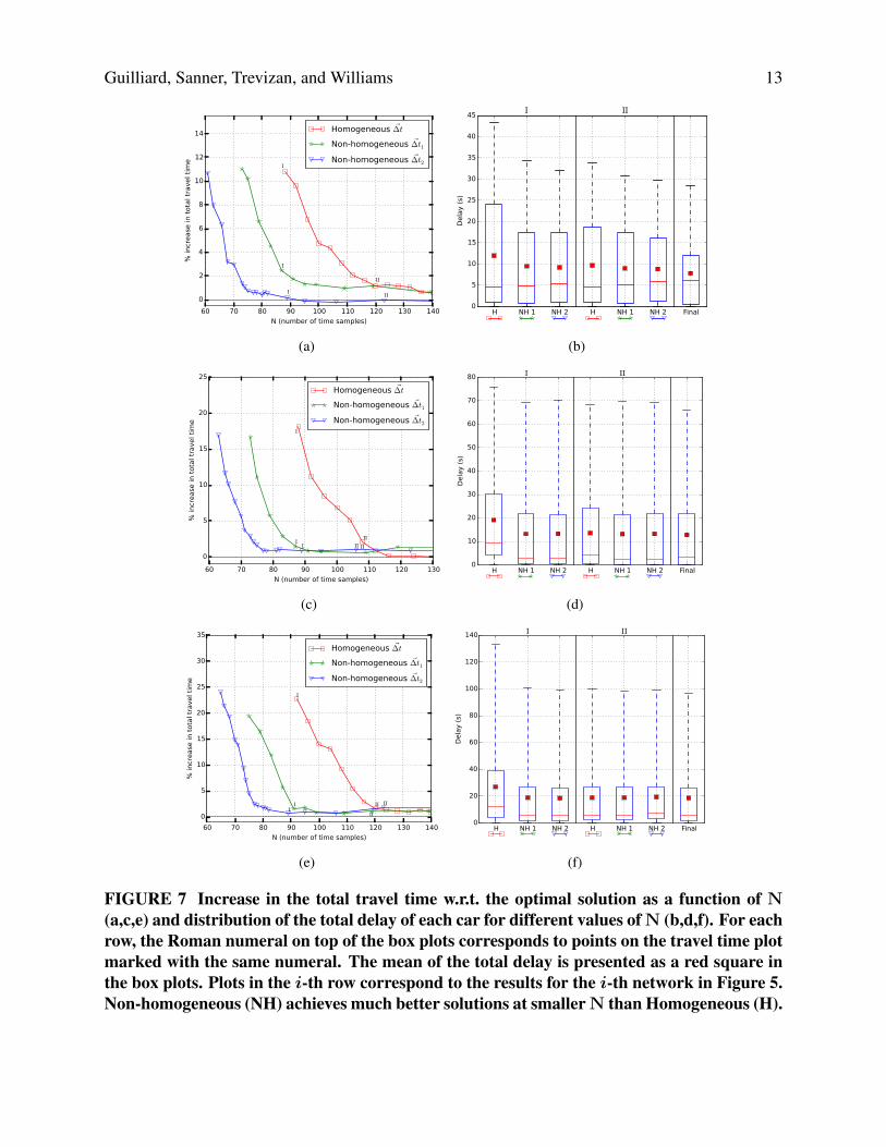
(e) (f)

FIGURE 7 Increase in the total travel time w.r.t. the optimal solution as a function of N(a,c,e) and distribution of the total delay of each car for different values of N (b,d,f). For eachrow, the Roman numeral on top of the box plots corresponds to points on the travel time plotmarked with the same numeral. The mean of the total delay is presented as a red square inthe box plots. Plots in the i-th row correspond to the results for the i-th network in Figure 5.Non-homogeneous (NH) achieves much better solutions at smaller N than Homogeneous (H).


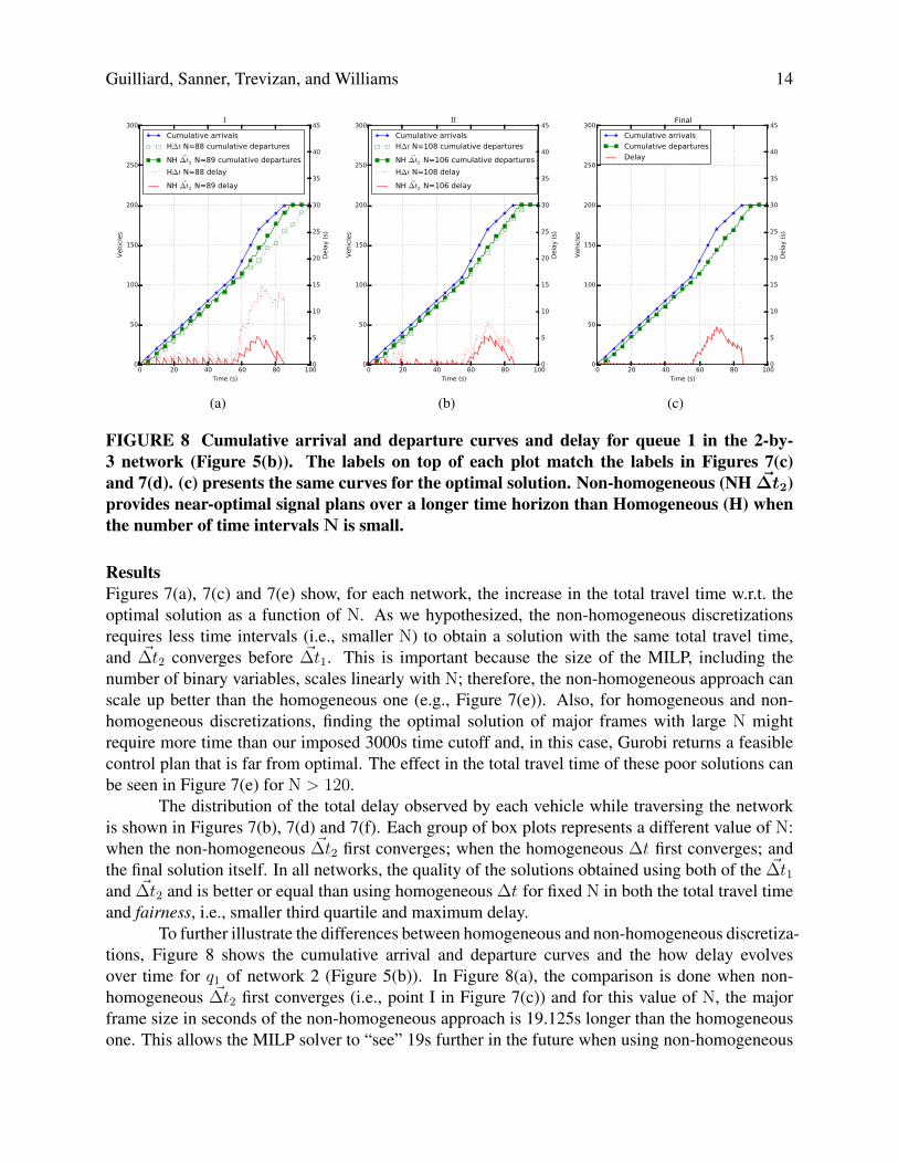
(a) (b) (c)

FIGURE 8 Cumulative arrival and departure curves and delay for queue 1 in the 2-by-3 network (Figure 5(b)). The labels on top of each plot match the labels in Figures 7(c)and 7(d). (c) presents the same curves for the optimal solution. Non-homogeneous (NH ~�t

2

)provides near-optimal signal plans over a longer time horizon than Homogeneous (H) whenthe number of time intervals N is small.

ResultsFigures 7(a), 7(c) and 7(e) show, for each network, the increase in the total travel time w.r.t. theoptimal solution as a function of N. As we hypothesized, the non-homogeneous discretizationsrequires less time intervals (i.e., smaller N) to obtain a solution with the same total travel time,and ~

�t

2

converges before ~

�t

1

. This is important because the size of the MILP, including thenumber of binary variables, scales linearly with N; therefore, the non-homogeneous approach canscale up better than the homogeneous one (e.g., Figure 7(e)). Also, for homogeneous and non-homogeneous discretizations, finding the optimal solution of major frames with large N mightrequire more time than our imposed 3000s time cutoff and, in this case, Gurobi returns a feasiblecontrol plan that is far from optimal. The effect in the total travel time of these poor solutions canbe seen in Figure 7(e) for N > 120.

The distribution of the total delay observed by each vehicle while traversing the networkis shown in Figures 7(b), 7(d) and 7(f). Each group of box plots represents a different value of N:when the non-homogeneous ~

�t

2

first converges; when the homogeneous �t first converges; andthe final solution itself. In all networks, the quality of the solutions obtained using both of the ~

�t

1

and ~

�t

2

and is better or equal than using homogeneous�t for fixed N in both the total travel timeand fairness, i.e., smaller third quartile and maximum delay.

To further illustrate the differences between homogeneous and non-homogeneous discretiza-tions, Figure 8 shows the cumulative arrival and departure curves and the how delay evolvesover time for q

1

of network 2 (Figure 5(b)). In Figure 8(a), the comparison is done when non-homogeneous ~

�t

2

first converges (i.e., point I in Figure 7(c)) and for this value of N, the majorframe size in seconds of the non-homogeneous approach is 19.125s longer than the homogeneousone. This allows the MILP solver to “see” 19s further in the future when using non-homogeneous


discretization and find a coordinated signal policy along the avenue to dissipate the extra trafficthat arrives at time 55s. The shorter major frame of the homogeneous discretization does not allowthe solver to adapt this far in advance and its delay observed after 55s is much larger than thenon-homogeneous one. Once the homogeneous �t has converged (Figure 8(b)), it is also able toanticipate the increased demand and adapt well in advance and both approaches generate solutionsclose to optimum (Figure 8(c)).

CONCLUSIONIn this paper, we showed how to formulate a novel queue transmission model (QTM) of trafficflow with non-homogeneous time steps as a linear program. We then proceeded to allow the traf-fic signals to become discrete variables subject to a delay minimizing optimization objective andstandard traffic signal constraints leading to a final MILP formulation of traffic signal control withnon-homogeneous time steps. We experimented with this novel QTM-based MILP control in arange of traffic networks and demonstrated that the non-homogeneous MILP formulation achieved(i) substantially lower delay solutions, (ii) improved per-vehicle delay distributions, and (iii) moreoptimal travel times over a longer horizon in comparison to the homogeneous MILP formulationwith the same number of binary and continuous variables. Altogether, this work represents a majorstep forward in the scalability of MILP-based jointly optimized traffic signal control via the use ofa non-homogeneous time traffic models and thus helps pave the way for fully optimized joint urbantraffic signal controllers as an improved successor technology to existing signal control methods.

Our future work includes learning the QTM parameters (e.g., turn probabilities Pr

i,j

andexpected incoming flows I

i,n

) from loop detector data, and evaluating the impact in scalability ofdifferent non-homogeneous discretizations and size of the computer cluster used for computing thecontrol plans.

ACKNOWLEDGMENTThis work is part of the Advanced Data Analytics in Transport programme, and supported by Na-tional ICT Australia (NICTA) and NSW Trade & Investment. NICTA is funded by the AustralianGovernment through the Department of Communications and the Australian Research Councilthrough the ICT Centre of Excellence Program. NICTA’s role is to pursue potentially economi-cally significant ICT related research for the Australian economy. NSW Trade & Investment is thebusiness development agency for the State of New South Wales.

REFERENCES[1] Bazzan, A. L. C. and F. Klügl, Introduction to Intelligent Systems in Traffic and Transporta-

tion. Synthesis Lectures on Artificial Intelligence and Machine Learning, Morgan & ClaypoolPublishers, 2013.

[2] El-Tantawy, S., B. Abdulhai, and H. Abdelgawad, Multiagent reinforcement learning forintegrated network of adaptive traffic signal controllers (MARLIN-ATSC): methodologyand large-scale application on downtown Toronto. Intelligent Transportation Systems, IEEETransactions on, Vol. 14, No. 3, 2013, pp. 1140–1150.

[3] Sims, A. G. and K. W. Dobinson, SCAT–The Sydney co-ordinated adaptive traffic system:Philosophy and benefits. IEEE Transactions on Vehicular Technology, Vol. 29, 1980.


[4] Hunt, P. B., D. I. Robertson, R. D. Bretherton, and R. I. Winton, SCOOT–A traffic responsivemethod of coordinating signals. Transportation Road Research Lab, Crowthorne, U.K., 1981.

[5] Gartner, N., J. D. Little, and H. Gabbay, Optimization of traffic signal settings in networks bymixed-integer linear programming. DTIC Document, 1974.

[6] Gartner, N. H. and C. Stamatiadis, Arterial-based control of traffic flow in urban grid net-works. Mathematical and computer modelling, Vol. 35, No. 5, 2002, pp. 657–671.

[7] Lo, H. K., A novel traffic signal control formulation. Transportation Research Part A: Policyand Practice, Vol. 33, No. 6, 1998, pp. 433–448.

[8] He, Q., K. L. Head, and J. Ding, PAMSCOD: Platoon-based Arterial Multi-modal SignalControl with Online Data. Procedia-Social and Behavioral Sciences, Vol. 17, 2011, pp. 462–489.

[9] Lin, W.-H. and C. Wang, An enhanced 0-1 mixed-integer LP formulation for traffic signalcontrol. Intelligent Transportation Systems, IEEE Transactions on, Vol. 5, No. 4, 2004, pp.238–245.

[10] Han, K., T. L. Friesz, and T. Yao, A link-based mixed integer LP approach for adaptive trafficsignal control. arXiv preprint arXiv:1211.4625, 2012.

[11] Lo, H. K., E. Chang, and Y. C. Chan, Dynamic network traffic control. Transportation Re-search Part A: Policy and Practice, Vol. 35, No. 8, 1999, pp. 721–744.

[12] He, Q., W.-H. Lin, H. Liu, and K. L. Head, Heuristic algorithms to solve 0–1 mixed integerLP formulations for traffic signal control problems. In Service Operations and Logistics andInformatics (SOLI), 2010 IEEE International Conference on, IEEE, 2010, pp. 118–124.

[13] Varaiya, P., Max pressure control of a network of signalized intersections. TransportationResearch Part C: Emerging Technologies, Vol. 36, 2013, pp. 177–195.

[14] Li, J. and H. Zhang, Coupled Linear Programming Approach for Decentralized Control of Ur-ban Traffic. Transportation Research Record: Journal of the Transportation Research Board,, No. 2439, 2014, pp. 83–93.

[15] Xie, X.-F., S. F. Smith, and G. J. Barlow, Schedule-Driven Coordination for Real-Time TrafficNetwork Control. In ICAPS, 2012.

[16] Smith, S., G. Barlow, X.-F. Xie, and Z. Rubinstein, SURTRAC: Scalable Urban Traffic Con-trol. In Transportation Research Board 92nd Annual Meeting Compendium of Papers, Trans-portation Research Board, 2013.

[17] Daganzo, C. F., The cell transmission model: A dynamic representation of highway trafficconsistent with the hydrodynamic theory. Transportation Research Part B: Methodological,Vol. 28, No. 4, 1994, pp. 269–287.

[18] Daganzo, C. F., The cell transmission model, part II: network traffic. Transportation ResearchPart B: Methodological, Vol. 29, No. 2, 1995, pp. 79–93.


[19] Xiaojian, H., W. Wei, and H. Sheng, Urban traffic flow prediction with variable cell trans-mission model. Journal of Transportation Systems Engineering and Information Technology,Vol. 10, No. 4, 2010, pp. 73–78.

[20] Sumalee, A., R. Zhong, T. Pan, and W. Szeto, Stochastic cell transmission model (SCTM): Astochastic dynamic traffic model for traffic state surveillance and assignment. TransportationResearch Part B: Methodological, Vol. 45, No. 3, 2011, pp. 507–533.

[21] Jabari, S. E. and H. X. Liu, A stochastic model of traffic flow: Theoretical foundations.Transportation Research Part B: Methodological, Vol. 46, No. 1, 2012, pp. 156–174.

[22] Huang, K. C., Traffic Simulation Model for Urban Networks: CTM-URBAN. Ph.D. thesis,Concordia University, 2011.

[23] Muralidharan, A., G. Dervisoglu, and R. Horowitz, Freeway traffic flow simulation using thelink node cell transmission model. In American Control Conference, 2009. ACC’09., IEEE,2009, pp. 2916–2921.

[24] Gomes, G. and R. Horowitz, Optimal freeway ramp metering using the asymmetric cell trans-mission model. Transportation Research Part C: Emerging Technologies, Vol. 14, No. 4,2006, pp. 244–262.

[25] Kim, Y., Online traffic flow model applying dynamic flow-density relation. Int. At. EnergyAgency, 2002.

[26] Lu, S., S. Dai, and X. Liu, A discrete traffic kinetic model–integrating the lagged cell trans-mission and continuous traffic kinetic models. Transportation Research Part C: EmergingTechnologies, Vol. 19, No. 2, 2011, pp. 196–205.

[27] Alecsandru, C., A. Quddus, K. C. Huang, B. Rouhieh, A. R. Khan, and Q. Zeng, An as-sessment of the cell-transmission traffic flow paradigm: Development and applications. InTransportation Research Board 90th Annual Meeting, 2011, 11-1152.

Date post:	01-May-2018
Category:	Documents
Upload:	dinhkhuong
View:	220 times
Download:	1 times

A Non-homogeneous Time Mixed Integer LP Formulation...

Documents