A NONLINEAR ELIMINATION PRECONDITIONED INEXACT NEWTON METHOD FOR HETEROGENEOUS HYPERELASTICITY * SHIHUA GONG † AND XIAO-CHUAN CAI ‡ Abstract. We propose and study a nonlinear elimination preconditioned inexact Newton method for the numerical simulation of diseased human arteries with a heterogeneous hyperelas- tic model. We assume the artery is made of layers of distinct tissues and also contains plaque. Traditional Newton methods often work well for smooth and homogeneous arteries, but suffer from slow or no convergence due to the heterogeneousness of diseased soft tissues when the material is quasi-incompressible. The proposed nonlinear elimination method adaptively finds a small number of equations causing the nonlinear stagnation and then eliminates them from the global nonlinear system. By using the theory of affine invariance of Newton method, we provide insight into why the nonlinear elimination method can improve the convergence of Newton iterations. Our numerical results show that the combination of nonlinear elimination with an initial guess interpolated from a coarse level solution can lead to the uniform convergence of Newton method for this class of very difficult nonlinear problems. Key words. Finite elements, nonlinearly preconditioned Newton method, hyperelasticity, arte- rial walls AMS subject classifications. 65F08, 65N55, 65N22, 74S05 1. Introduction. Nonlinearly preconditioned inexact Newton algorithms [7, 8, 14, 15] have been applied with significant success to solve difficult nonlinear problems in computational fluid dynamics involving boundary layers, local singularities or shock waves. In this paper, we consider applying nonlinear preconditioning techniques to solve a heterogeneous hyperelastic problem arising from the modeling of diseased arteries. Arterial walls are composed of three distinct tissue layers from inside to outside: the intima, the media, and the adventitia. The mechanical properties of the intima can be negligible. The other two layers can be modeled as fiber-enforced materials composed of a nearly incompressible matrix embeded with collagen fibers. For the disease of atherosclerosis, some plaque components of calcification and lipids may build up inside the arteries. In [6], the authors consider several material models for diseased arterial walls in order to study the mechanical response and the influence on the nonlinear iterations. It is reported that both the heterogeneousness of diseased soft tissues and the quasi-incompressibility have negative effects on the convergence of Newton method. To accelerate the convergence of Newton iteration, nonlinear preconditioning is introduced as a built-in machinery for the inexact Newton algorithm (IN) [9, 11] in order to deal with the unbalanced nonlinearities. It can be applied on the left or on the right of the nonlinear function. The additive Schwarz preconditioned inexact Newton algorithm (ASPIN) [7] is an example of the left preconditioning, and was observed in [7] to provide a more “balanced” system. On the other hand, right preconditioning techniques such as nonlinear elimination (NE) [8, 14, 15, 20] effectively modifies the variables of the nonlinear system. NE is easier to implement than ASPIN since the nonlinear function does not have to be changed and the nonlinear elimination step * The work of the first author was supported in part by National Natural Science Foundation of China No.91430215. The work of the second author was supported in part by NSF DMS-1720366. † Department of Mathematical Sciences, University of Bath, Bath BA2 7AY, UK. ‡ Department of Computer Science, University of Colorado Boulder, Boulder, CO 80309, USA, ([email protected]). 1
Transcript
A NONLINEAR ELIMINATION PRECONDITIONED INEXACTNEWTON METHOD FOR HETEROGENEOUS HYPERELASTICITY∗
SHIHUA GONG† AND XIAO-CHUAN CAI‡
Abstract. We propose and study a nonlinear elimination preconditioned inexact Newtonmethod for the numerical simulation of diseased human arteries with a heterogeneous hyperelas-tic model. We assume the artery is made of layers of distinct tissues and also contains plaque.Traditional Newton methods often work well for smooth and homogeneous arteries, but suffer fromslow or no convergence due to the heterogeneousness of diseased soft tissues when the material isquasi-incompressible. The proposed nonlinear elimination method adaptively finds a small numberof equations causing the nonlinear stagnation and then eliminates them from the global nonlinearsystem. By using the theory of affine invariance of Newton method, we provide insight into whythe nonlinear elimination method can improve the convergence of Newton iterations. Our numericalresults show that the combination of nonlinear elimination with an initial guess interpolated froma coarse level solution can lead to the uniform convergence of Newton method for this class of verydifficult nonlinear problems.
1. Introduction. Nonlinearly preconditioned inexact Newton algorithms [7, 8,14, 15] have been applied with significant success to solve difficult nonlinear problemsin computational fluid dynamics involving boundary layers, local singularities or shockwaves. In this paper, we consider applying nonlinear preconditioning techniques tosolve a heterogeneous hyperelastic problem arising from the modeling of diseasedarteries. Arterial walls are composed of three distinct tissue layers from inside tooutside: the intima, the media, and the adventitia. The mechanical properties ofthe intima can be negligible. The other two layers can be modeled as fiber-enforcedmaterials composed of a nearly incompressible matrix embeded with collagen fibers.For the disease of atherosclerosis, some plaque components of calcification and lipidsmay build up inside the arteries. In [6], the authors consider several material modelsfor diseased arterial walls in order to study the mechanical response and the influenceon the nonlinear iterations. It is reported that both the heterogeneousness of diseasedsoft tissues and the quasi-incompressibility have negative effects on the convergenceof Newton method.
To accelerate the convergence of Newton iteration, nonlinear preconditioning isintroduced as a built-in machinery for the inexact Newton algorithm (IN) [9, 11] inorder to deal with the unbalanced nonlinearities. It can be applied on the left or on theright of the nonlinear function. The additive Schwarz preconditioned inexact Newtonalgorithm (ASPIN) [7] is an example of the left preconditioning, and was observed in[7] to provide a more “balanced” system. On the other hand, right preconditioningtechniques such as nonlinear elimination (NE) [8, 14, 15, 20] effectively modifies thevariables of the nonlinear system. NE is easier to implement than ASPIN since thenonlinear function does not have to be changed and the nonlinear elimination step
∗The work of the first author was supported in part by National Natural Science Foundation ofChina No.91430215. The work of the second author was supported in part by NSF DMS-1720366.†Department of Mathematical Sciences, University of Bath, Bath BA2 7AY, UK.‡Department of Computer Science, University of Colorado Boulder, Boulder, CO 80309, USA,
doesn’t have to be called at every outer Newton iteration. Moreover, more efficientand sophisticated linear solvers can be applied to the unchanged Jacobian.
An early work on NE is presented in [20], where the authors discussed how NEcan retain the higher-order convergence of Newton method near the root of the sys-tem of nonlinear equations. It is still a nontrivial task to choose some subfunctions orvariables to eliminate such that the convergence of Newton method becomes faster.For some computational fluid dynamics problems, the robustness and the effectivenessof NE are demonstrated in [14, 15]. Here the NE is applied to those variables withhigh local nonlinearity as characterized by the local Lipschitz constant. The nonlin-ear FETI-DP (Finite Element Tearing and Interconnecting Dual-Primal) and BDDC(Balancing Domain Decomposition by Constraint) [16, 17, 18] domain decompositionmethods also use the concept of NE and obtain satisfying parallel scalability usingdifferent nonlinear elimination strategies.
However, a straightforward application of NE to hyperelasticity does not work wellprobably because it introduces sharp jumps in the residual near the boundary of theeliminating subdomains. We refer to this as the thrashing phenomenon. Such jumpsdeteriorate the performance of nonlinear preconditioning. To resolve this problem,we use the theory of affine invariance [10] to analyze the convergence of the dampedNewton method with exact nonlinear elimination, and then provide some insight intohow to design the nonlinear elimination preconditioner. Our proposed algorithm is atwo-level method with two key components: an adaptive nonlinear elimination schemeand a nodal-value interpolation operator. The interpolation operator provides an ini-tial guess with a coarse level approximation to deal with the global nonlinearity. Notethat, for quasi-incompressible linear elasticity, the nodal interpolation is unstable sinceit does not preserve the volume. Thus, the inexact Newton method fails even withan initial guess interpolated from a coarse level solution, which is observed from ournumerical experiments. Another reason for this may be due to the different geometryapproximations by different level meshes for a curved domain. The interpolation mayintroduce local pollution to the initial guess. Whereas, with the help of an adaptivenonlinear elimination scheme, we can capture the local pollution causing unbalancednonlinearity and then eliminate it from the global system. We numerically show thatthis combination leads to a uniform convergence for Newton iterations.
The rest of the paper is organized as follows. We present the model and the dis-cretization for arterial walls in Section 2. The nonlinear elimination preconditionedNewton method is proposed and discussed in Section 3. In Section 4, some numericalexperiments are presented to demonstrate the performance of the nonlinear elimina-tion preconditioning. The concluding remarks are given in the last section.
2. Model and discretization. We consider a hyperelastic model for arterialwalls and its finite element discretization. First, we introduce some basic notationsin continuum mechanics. The body of interest in the reference configuration is de-noted by Ω ∈ R3, parameterized by X, and the current configuration by Ω ∈ R3,parametrized by x. The deformation map φ(X) = X + u : Ω 7→ Ω is a differentialisomorphism between the reference and current configuration. Here u is the displace-ment defined on the reference configuration. The deformation gradient F is definedby
F (X) = ∇φ(X) = I +∇u,
with the Jacobian J(X) = detF (X) > 0. The right Cauchy-Green tensor is definedby
C = F TF .
NONLINEAR ELIMINATION PRECONDITIONED NEWTON METHOD 3
The hyperelastic materials postulate the existence of an energy density functionψ defined per unit reference volume. By the principle of material frame indifference[19], one can prove that the energy function is a function of C, i.e., ψ = ψ(C). Basedon a specific form of the energy function, the first and second Piola-Kirchhoff stresstensor are
P = FS and S = 2∂ψ
∂C.
And the Cauchy stress is given by σ = J−1FSF T . The balance of the momentum isgoverned by the following hyperelastic equation
(2.1)
−div(FS) = f, on Ω,
u = u, on Γg,
PN = t, on Γh,
where f is the body force vector, N denotes unit exterior normal to the boundarysurface Γh and ∂Ω = Γg ∪ Γh with Γg ∩ Γh = ∅. In the rest of the paper, we alwaysconsider homogeneous Dirichlet boundary condition u = 0 and the situation wherethe deformation is driven by external applied pressure load. The simple pressureboundary condition is a distributed load normal to the applied surface in the referenceconfiguration; reads as t = −pN. We are also interested in the follower pressure load[5], which is applied to the current deformed state; reads as
t = −p(cofF )N.
Here cofF = JF−T is the cofactor of F . It concerns the change in direction of thenormals as well as the area change. The dependence on the deformed geometry makesthis a nonlinear boundary condition, which brings extra challenge for the convergenceof the nonlinear solvers.
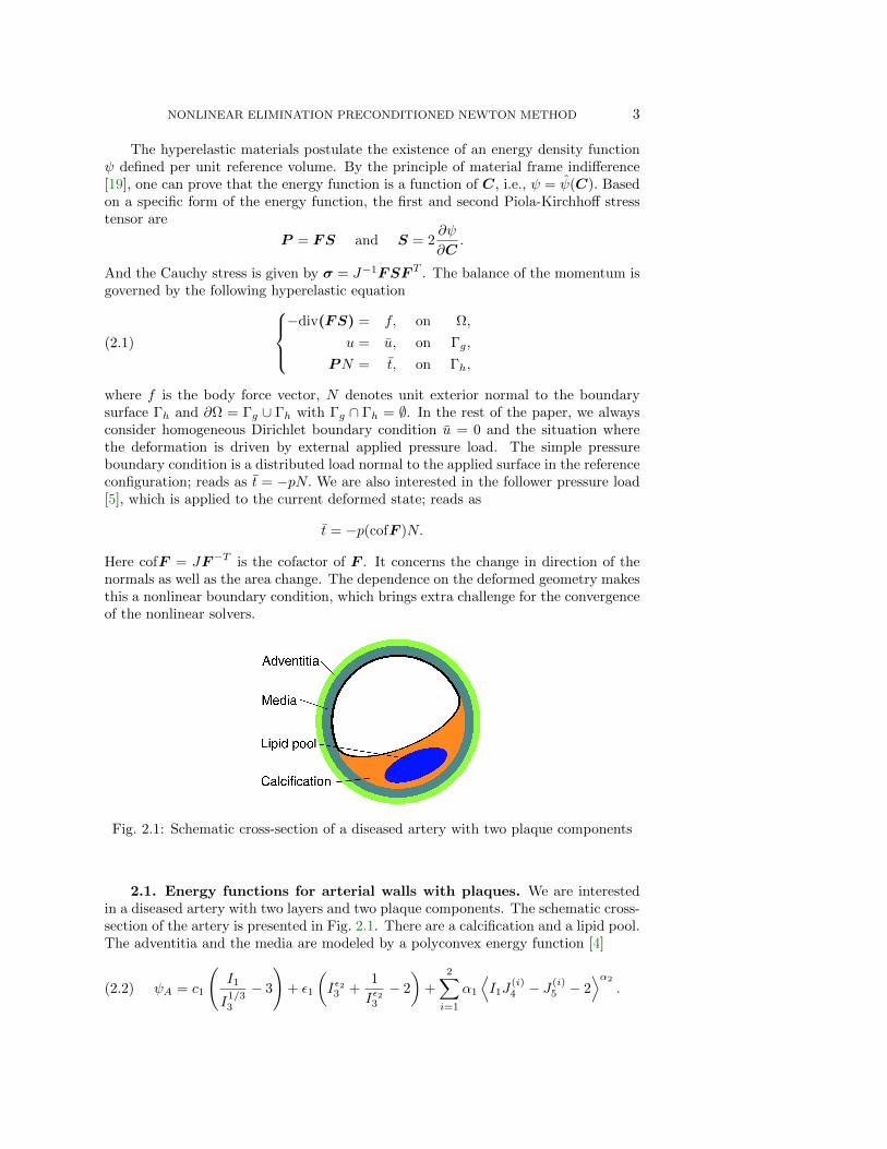
Fig. 2.1: Schematic cross-section of a diseased artery with two plaque components
2.1. Energy functions for arterial walls with plaques. We are interestedin a diseased artery with two layers and two plaque components. The schematic cross-section of the artery is presented in Fig. 2.1. There are a calcification and a lipid pool.The adventitia and the media are modeled by a polyconvex energy function [4]
(2.2) ψA = c1
(I1
I1/33
− 3
)+ ε1
(Iε23 +
1
Iε23
− 2
)+
2∑i=1
α1
⟨I1J
(i)4 − J
(i)5 − 2
⟩α2
.
4 SHIHUA GONG AND XIAO-CHUAN CAI
Here, 〈b〉 denotes the Macaulay brackets defined by 〈b〉 = (|b|+ b)/2, with b ∈ R. AndI1, I2, I3 are the principal invariants of C; i.e.,
I1 := tr(C), I2 := tr(cofC), I3 := detC.
The additional mixed invariants J(i)4 , J
(i)5 characterize the anisotropic behavior of
arterial wall and are defined as J(i)4 = tr[CM (i)], J
(i)5 := tr[C2M (i)], i = 1 : 2, where
M (i) := a(i) ⊗ a(i) are the structural tensors with a(i), i = 1, 2 denoting the directionfields of the embedded collagen fibers. This is based on the fact that only weakinteractions between the two fibre directions are observed; for further arguments, see[13]. The polyconvexity condition in the sense of [2] is the essential condition to ensurethe existence of energy minimizers and the material stability.
Following [6], the lipid is modeled by the isotropic part of ψA used for the ad-ventitia and media. The calcification area is modeled as an isotropic Mooney-Rivlinmaterial with the following energy function
ψC = β1I1 + η1I2 + δ1I3 − δ2 ln I3.
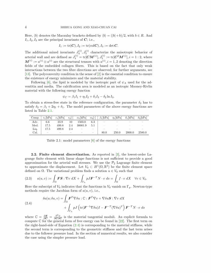
To obtain a stress-free state in the reference configuration, the parameter δ2 has tosatisfy δ2 = β1 + 2η1 + δ1. The model parameters of the above energy functions arelisted in Table 2.1.
Table 2.1: model parameters [6] of the energy functions
2.2. Finite element discretization. As reported in [3], the lowest-order La-grange finite element with linear shape functions is not sufficient to provide a goodapproximation for the arterial wall stresses. We use the P2 Lagrange finite elementto approximate the displacement. Let V0 ⊂ H1(Ω,R3) be the finite element spacedefined on Ω. The variational problem finds a solution u ∈ V0 such that
(2.3) a(u, v) :=
∫Ω
FS : ∇v dX +
∫Γh
pJF−TN · v ds =
∫Ω
f · v dX ∀v ∈ V0.
Here the subscript of V0 indicates that the functions in V0 vanish on Γg. Newton-typemethods require the Jacobian form of a(u, v), i.e.,
(2.4)
δa(u; δu, v) =
∫Ω
F T∇δu : C : F T∇v +∇δuS : ∇v dX
+
∫Γh
pJ(
tr(F−1∇δu)I − F−T (∇δu)T)F−TN · v ds
where C = ∂S∂C = ∂2ψ
∂C∂C is the material tangential moduli. An explicit formula tocompute C for the general form of free energy can be found in [22]. The first term onthe right-hand-side of Equation (2.4) is corresponding to the material stiffness, whilethe second term is corresponding to the geometric stiffness and the last term arisesdue to the follower pressure load. In the section of numerical results, we also considerthe case using the simpler pressure load.
NONLINEAR ELIMINATION PRECONDITIONED NEWTON METHOD 5
3. Inexact Newton method with nonlinear elimination precondition-ing. In this section, we first describe the motivation of nonlinear preconditioningbased on an affine invariant convergence theorem of Newton-type methods. Afterthat, we analyze the precondtioning effect of nonlinear elimination and then givea detailed description of the nonlinear elimination preconditioned inexact Newtonmethod (NEPIN).
We rewrite (2.3) as a system of n equations
(3.1) F (u∗) = 0,
where F ∈ C1(D), F : D 7→ Rn with an n by n Jacobian J = F ′(u) and D ⊂ Rn openand convex. Given an initial guess u0 of a solution u∗, the damped Newton methodfinds a sequence of iterates uk computed through
(3.2) F ′(uk)pk = −F (uk),
(3.3) uk+1 = uk + λkpk, λk ∈ (0, 1]
Here pk is the Newton direction and λk is a scalar determined by a monotonicity testsuch that
(3.4) T (uk+1) ≤ θT (uk),
where θ ∈ (0, 1) and T (u) is a level function measuring how close u is to the solutionu∗. In most cases, one sets T (u) = 1
2‖F (u)‖22. We use ‖ · ‖ to denote a generic normand ‖ · ‖p for the `p-norm.
The convergence of uk to u∗ is quadratic if the initial guess is close enough tothe desired solution and λk → 1. However, a good initial guess is generally unavailableand the monotonicity test (3.4) often results in a really small step length λk. Thisphenomenon is described rigorously in the Theorem 3.1 under the framework of affineinvariance [10] with a localized version of the affine contravariant Lipschitz condition.The first assumption of our analysis is given as follows:
Assumption 1. Assume the affine contravariant Lipschitz condition holds
(3.5) ‖ (F ′(v)− F ′(u)) (v − u)‖ ≤ ωF ‖F ′(u)(v − u)‖2, for any v, u ∈ D.
Here we call ωF a global affine contravriant Lipschitz constant.
Let p be the Newton direction of F at u and set v − u = λp in (3.5) for anyλ ∈ (0, 1]. Thus, for any u ∈ D and λ ∈ (0, 1], let ωF,u,λ be the minimum constantsuch that
Here we call ωF,u,λ a local affine contravriant Lipschitz constant. We also denoteωF,u = supλ∈(0,1] ωF,u,λ and ωF = supu∈D ωF,u. Note that ωF,u,λ ≤ ωF by Assump-tion 1. Thus, the supremums ωF,u and ωF taken over a set of values bounded fromabove are well-defined.
Theorem 3.1. Let F ′(u) be nonsingular for all u ∈ D and Assumption 1 holds.With the notation hk := ωF,uk‖F (uk)‖, and λ ∈ (0,min(1, 2/hk)], we have
(3.7) ‖F (uk + λpk)‖ ≤ tk(λ)‖F (uk)‖,
6 SHIHUA GONG AND XIAO-CHUAN CAI
where tk(λ) := 1− λ+ 12λ
2hk. Moreover, if hk < 2, we have
(3.8) ‖F (uk + pk)‖ ≤ 1
2ωF ‖F (uk)‖2.
Proof. The proof here is presented for completeness; see [10] for the original one.By applying the Newton-Leibniz formula and Assumption 1, we obtain the estimate(3.7):
‖F (uk + λpk)‖ = ‖F (uk) +
∫ λ
t=0
F ′(uk + tp)p dt‖
= ‖(1− λ)F (uk) +
∫ λ
t=0
(F ′(uk + tpk)− F ′(uk)
)pk dt‖
≤ ‖(1− λ)F (uk)‖+
∫ λ
t=0
tωF,uk‖F (uk)‖2 dt
= (1− λ+1
2λ2hk)‖F (uk)‖
To get a reduction on the norm of residual, the step length should be chosen in theinterval (0,min(1, 2/hk)]. Moreover, if hk < 2, let λ = 1 and then we obtain thequadratic convergence (3.8).
According to the theorem, the convergence is quadratic when hk < 2. For hk ≥ 2,the optimal step size is λk := 1
hk. And then the optimal reduction rate of the residual,
i.e., the minimal value of tk(λ) in (3.7), is tk := 1 − 12hk
. If hk has a uniform upperbound for all k, then the convergence of the damped Newton iteration would beacceptable.
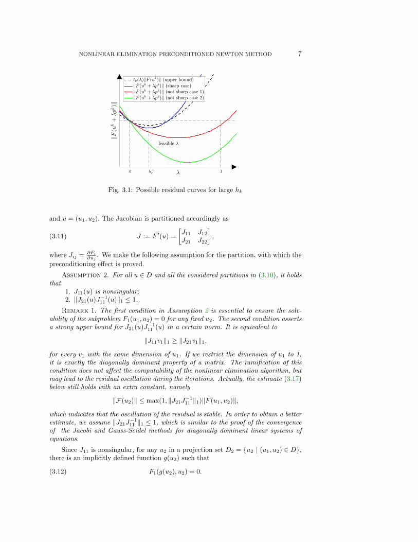
However, if there are some iterations for which hk is too large, stagnation in thenonlinear iteration may occur. Our main objective is to introduce a built-in machinery(nonlinear preconditioning) to prevent the stagnation. The nonlinear residual curvebehaves in several different ways:
• The estimate (3.7) is sharp; see the blue curve in Fig. 3.1. The feasible stepsize λ that satisfies the monotonicity test (3.4) should be very small, and ourtheoretical analysis applies well in such a situation.
• The estimate (3.7) is not sharp; see the red and green curves in Fig. 3.1. Forthe green one, there is no stagnation. For the red one, stagnation occurs andwe need to apply nonlinear preconditioning, but our analysis is not able toexplain the performance of the algorithm.
Based on the above discussion, an intuitive idea to precondition Newton method(to prevent the stagnation) is to make the quantity
(3.9) hk := ωF,uk‖F (uk)‖
smaller. In the following, we transform the nonlinear function F (uk) to F(uk) vianonlinear elimination. Under appropriate assumptions, we prove that the local affinecontravariant Lipschitz constant ωF,uk,λ of F as well as the new residual ‖F(uk)‖ issmaller than that of the original nonlinear function F (uk).
3.1. Exact nonlinear elimination. Assume F (u) is partitioned as
(3.10) F (u) =
[F1(u1, u2)F2(u1, u2)
],
NONLINEAR ELIMINATION PRECONDITIONED NEWTON METHOD 7
Fig. 3.1: Possible residual curves for large hk
and u = (u1, u2). The Jacobian is partitioned accordingly as
(3.11) J := F ′(u) =
[J11 J12
J21 J22
],
where Jij = ∂Fi∂uj
. We make the following assumption for the partition, with which the
preconditioning effect is proved.
Assumption 2. For all u ∈ D and all the considered partitions in (3.10), it holdsthat
1. J11(u) is nonsingular;2. ‖J21(u)J−1
11 (u)‖1 ≤ 1.
Remark 1. The first condition in Assumption 2 is essential to ensure the solv-ability of the subproblem F1(u1, u2) = 0 for any fixed u2. The second condition assertsa strong upper bound for J21(u)J−1
11 (u) in a certain norm. It is equivalent to
‖J11v1‖1 ≥ ‖J21v1‖1,
for every v1 with the same dimension of u1. If we restrict the dimension of u1 to 1,it is exactly the diagonally dominant property of a matrix. The ramification of thiscondition does not affect the computability of the nonlinear elimination algorithm, butmay lead to the residual oscillation during the iterations. Actually, the estimate (3.17)below still holds with an extra constant, namely
‖F(u2)‖ ≤ max(1, ‖J21J−111 ‖1)‖F (u1, u2)‖,
which indicates that the oscillation of the residual is stable. In order to obtain a betterestimate, we assume ‖J21J
−111 ‖1 ≤ 1, which is similar to the proof of the convergence
of the Jacobi and Gauss-Seidel methods for diagonally dominant linear systems ofequations.
Since J11 is nonsingular, for any u2 in a projection set D2 = u2 | (u1, u2) ∈ D,there is an implicitly defined function g(u2) such that
(3.12) F1(g(u2), u2) = 0.
8 SHIHUA GONG AND XIAO-CHUAN CAI
Then our preconditioned nonlinear problem reads as: finding u2 such that
(3.13) F(u2) := F2(g(u2), u2) = 0.
We call u = (g(u2), u2) as the cut-extension of u2. Next, we analyze the convergenceof Newton method applied to the preconditioned system.
To derive the Jacobian of F , one can first take the derivative of (3.12) with respectto u2 and then have J11g
′(u2) + J12 = 0. Since J11 is nonsingular, we have
(3.14) g′(u2) = −J−111 J12.
Then, by differentiating (3.13) and using (3.14), we have
Note that J (u2) is the Schur complement of J(u), where u = (g(u2), u2) is the cut-extension of u2. Let p2 := −J−1(u2)F(u2) be the Newton direction of F . We definea harmonic extension of p2 by p = (h(p2), p2) such that h(p2) satisfying
J11(u)h(p2) + J12(u)p2 = 0,
or equivalently h(p2) = g′(u2)p2. Thus, we have the linear approximation property
g(u2 + λp2) ≈ g(u2) + g′(u2)λp2 = g(u2) + λh(p2),
for sufficiently small λ.Moreover, one can show that p actually is the Newton direction of F at u since
(3.16) J(u)p =
[J11 J12
J21 J22
] [h(p2)p2
]=
[0
J (u2)p2
]=
[−F1 (g(u2), u2)−F2 (g(u2), u2)
]= −F (u).
Thus, we can obtain the precondtioned Newton direction p2 directly by solving theoriginal Jacobian system J(u)p = −F (u) without assembling the Schur complementJ (u2).
Lemma 3.2. If Assumption 2 holds, then for any u = (u1, u2) ∈ D, we have
NONLINEAR ELIMINATION PRECONDITIONED NEWTON METHOD 9
Lemma 3.3. If Assumption 2 holds, then for any u2 ∈ D2, we have
(3.18)‖(J (u2 + λp2)− J (u2))p2‖1
λ‖J (u2)p2‖21≤ ‖ (J(v)− J(u)) p‖1
λ‖J(u)p‖21.
Here p2 := −J−1(u2)F(u2) and p := −J−1(u)F (u) are the Newton directions of Fand F , respectively. And u := (g(u2), u2) and v := (g(u2 + λp2), u2 + λp2) are thecut-extension of u2 and u2 + λp2, respectively.
Proof. By (3.16), we have
(3.19) ‖J (u2)p2‖1 = ‖J up‖1.
Here we use the superscript u to indicate that the Jacobian is evaluated at u, i.e.,J u = J(g(u2), u2). Set v = (g(u2 + λp2), u2 + λp2) and v2 = u2 + λp2. We have
(3.21) ‖ (J (u2 + λp2)− J (u2)) p2‖1 ≤ ‖(J v − J u
)p‖1.
By (3.19) and (3.21), we complete the proof.
The analysis provides us some insight about how to design the nonlinear elimina-tion preconditioner:1. The nonlinear preconditioning effect. The convergence of Newton-type methods
relies on a certain form of Lipschitz condition. In (3.18) of Lemma 3.3, the left-hand side is a characterization of the affine contravariant Lipschitz constant of F .Whereas, for the right-hand side of F , it is not valid since the cut-extension
v :=
(g(u2 + λp2)u2 + λp2
)6= u+ λp =
(g(u2) + λh(p2)
u2 + λp2
).
However, we have g(u2 + λp2) = g(u2) + λh(p2) + O(λ2) and then v ≈ u + λp.Thus, let F be sufficiently smooth and by Lemma 3.3, we obtain, for small λ andin the sense of `1-norm,
ωF,u2,λ ≤ ωF,u,λ +O(λ).
If the stagnation in the nonlinear residual appears, Theorem 3.1 tells us that theoptimal step length λk = 1
hkshould be really small. In such situations, the non-
linear elimination accelerates the convergence of Newton iteration by making theresidual and the local affine contravariant Lipschitz constant smaller.
10 SHIHUA GONG AND XIAO-CHUAN CAI
2. How to perform nonlinear elimination? To apply a Newton step to the nonlinearelimination precondtioned system (3.13), one requires a solve of the Schur comple-ment system
J p2 = F
and several solves of g(u2 + λp2) during the line search step to satisfy
‖F(g(u2 + λp2), u2 + λp2)‖ ≤ θ‖F(g(u2), u2)‖.
This is often considered too expensive in realistic applications. Fortunately, accord-ing to our analysis, we can obtain the precondtioned Newton direction p2 directlyby solving the original Jacobian system
J(u)p = −F (u),
provided that F1(u) = F1(g(u2), u2) = 0. And then we have p = (h(p2), p2).Moreover, we have the approximation (g(u2 + λp2), u2 + λp2) ≈ u+ λp. Thus, theline search can be carried out approximately as
‖F (u+ λp)‖ ≤ θ‖F (u)‖.
From this point of view, the nonlinear elimination preconditioner only needs to up-date the approximate solution u = (u1, u2) to u = (g(u2), u2) before each Newtoniteration of the original problem, and the implementation of the Newton iterationdoes not change, including the assembling of the Jacobian matrix, the assemblingof the residual vector and the linear solver.
3. How to choose the eliminated equations? According to Lemma 3.2, the reductionrate on the residual is bounded by
‖F2‖1 + ‖J21J−111 ‖1‖F1‖1
‖F‖1.
Note that the subscripts in F1, F2, J11 and J21 correspond to a partition of the non-linear functions and variables. Assumption (2) ensures that there exists a uniformupper bound for ‖J21J
−111 ‖1 with respect to all partitions under consideration. If
the upper bound for ‖J21J−111 ‖1 is strictly smaller than 1, one should choose F1 to
be as large as possible such that these values are reduced through a multiplicationwith ‖J21J
−111 ‖1.
4. How to choose the eliminated variables? Assumption 2 asserts ‖J21J−111 ‖1 ≤ 1. A
weaker requirement is‖J21(u)‖1 ≤ ‖J11(u)‖1.
For some elliptic problems, it is usually satisfied due to the diagonally dominantproperty. In the cases of the finite element discretization, each equation is asso-ciated with a basis function and the variables are the coefficients of the solution.To maximize the norm ‖J11(u)‖1, one should choose the eliminated variables suchthat the eliminated equations and the eliminated variables are associated with thesame finite element basis functions. For the saddle-point problems, we should usesome point-block strategies, which means we group all physical components asso-ciated with a mesh point as a block and always perform elimination for this smallblock. This paper does not cover the point-block strategies; please see [14] for moredetails.
NONLINEAR ELIMINATION PRECONDITIONED NEWTON METHOD 11
3.2. Inexact nonlinear elimination. In this subsection, we first present abasic nonlinear solver: inexact Newton method (IN) [9, 11]. After that, we propose anonlinearity checking scheme to detect the eliminated equations and then embed thenonlinear elimination preconditioner into IN, which is briefly described here. Supposeuk is the current approximate solution, a new approximate solution uk+1 is computedthrough the following two steps
ALGORITHM 1 (IN).Step 1: Find the inexact Newton direction pk such that
‖F (uk) + F ′(uk)pk‖ ≤ max(ηa, ηr‖F (uk)‖),
Step 2: Compute the new approximate solution with suitable damping coefficient λk
uk+1 = uk + λkpk.
Here ηa and ηr ∈ [0, 1) are the absolute and relative tolerances that determinehow accurately the Jacobian system needs to be solved, and λk is another scalar thatdetermines how far one should go in the selected direction.
3.2.1. Nonlinearity checking and subproblem construction. As discussedfollowing the proof of Theorem 3.1, the nonlinear preconditioning is introduced toprevent the stagnation in the nonlinear iteration. Thus, before performing nonlinearelimination, we need to evaluate the local nonlinearity of the nonlinear function. Weuse the following criterion for the nonlinearity checking
‖F (uk)‖‖F (uk−1)‖
≤ ρrdt,
where ρrdt ∈ (0, 1) is a pre-chosen tolerance. If the reduction rate in the residual issmaller than ρrdt, the global inexact Newton iteration works well and the nonlinearelimination is not needed. Otherwise, we perform nonlinear elimination.
The nonlinear elimination substitutes the current guess uk by uk, which is ob-tained by solving a nonlinear subproblem. Next we construct the subproblem in analgebraic way. Let n be the size of the global nonlinear problem and
S = 1, · · · , n
be the global index set; i.e., one integer for each unknown ui and the correspondingFi. Note that, different to the subscripts in Section 3.1, here we abuse the notationof subscript to indicate a component of the vectors or the degree of freedom. Thefollowing index set collects the degrees of freedom with large residual components(which we call as bad components):
Sb := j ∈ S∣∣ |Fj(uk)| > ρres‖F (uk)‖∞.
Here ‖F (uk)‖∞ = maxni=1 |Fi(uk)| is the infinity norm taken over the global index setS and ρres ∈ (0, 1) is a pre-chosen tolerance.
According to our numerical tests, sharp jumps in the residual function would beintroduced if we only eliminate the equations and variables with indices in Sb. Atrick to prevent these jumps is to extend Sb to Sδb by adding the degrees of freedomwith overlapping δ to Sb. Here the overlapping δ is an integer corresponding to the
12 SHIHUA GONG AND XIAO-CHUAN CAI
connectivity in the graph characterized by the global Jacobian matrix. Thus, theresulting subspace is denoted by
V δb = v | v = (v1, · · · , vn)T ∈ Rn, vi = 0, if i 6∈ Sδ
b.
The corresponding restriction matrix is denoted by Rδb ∈ Rn×n, whose ith column iseither zero if i 6∈ Sδb or the ith column of the indentity matrix In×n.
Given an approximate solution uk and an index set Sδb , the nonlinear eliminationalgorithm finds the correction by approximately solving uδb ∈ V δb ,
(3.22) F δb (uδb) := RδbF (uδb + uk) = 0.
The new approximate solution is obtained as uk = uδb + uk. It is easy to see that the
Jacobian of (3.22) is Jδb (uδb) = RδbJ(uδb + u)(Rδb)T , where J = F ′ =
(∂Fi∂uj
)n×n
.
Before performing nonlinear elimination, we need to estimate the computationalcost for solving the subproblem (3.22). If the size of the subproblem is too large, itindicates that the residual is large in most of the domain and the current approximatesolution is really bad. We need to find a better initial guess or perform the globalinexact Newton iteration in such a situation. If the following condition is satisfied
#(Sδb ) < ρsizen,
we solve the subproblem (3.22) approximately such that
‖F δb (uδb)‖ ≤ max(γa, γr‖RδbF (uk)‖).
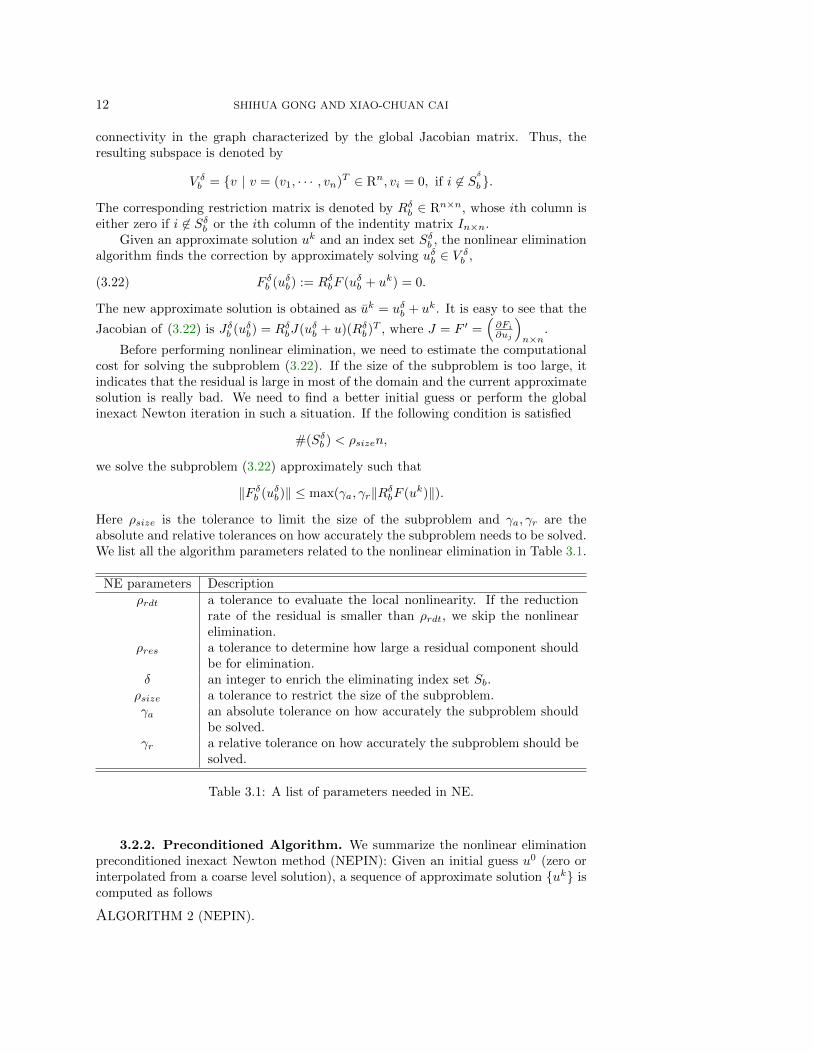
Here ρsize is the tolerance to limit the size of the subproblem and γa, γr are theabsolute and relative tolerances on how accurately the subproblem needs to be solved.We list all the algorithm parameters related to the nonlinear elimination in Table 3.1.
NE parameters Descriptionρrdt a tolerance to evaluate the local nonlinearity. If the reduction
rate of the residual is smaller than ρrdt, we skip the nonlinearelimination.
ρres a tolerance to determine how large a residual component shouldbe for elimination.
δ an integer to enrich the eliminating index set Sb.ρsize a tolerance to restrict the size of the subproblem.γa an absolute tolerance on how accurately the subproblem should
be solved.γr a relative tolerance on how accurately the subproblem should be
solved.
Table 3.1: A list of parameters needed in NE.
3.2.2. Preconditioned Algorithm. We summarize the nonlinear eliminationpreconditioned inexact Newton method (NEPIN): Given an initial guess u0 (zero orinterpolated from a coarse level solution), a sequence of approximate solution uk iscomputed as follows
ALGORITHM 2 (NEPIN).
NONLINEAR ELIMINATION PRECONDITIONED NEWTON METHOD 13
Step 1 Perform the nonlinearity checking:
1.1 If the reduction rate ‖F (uk)‖‖F (uk−1)‖ ≤ ρrdt, set uk = uk and go to Step 3.
1.2 Find the eliminated degrees of freedom and construct the index set Sδb .1.3 If #(Sδb ) < ρsizen, go to Step 2. Otherwise, set uk = uk and go to Step 3.
Step 2 Compute the correction uδb ∈ V δb by solving the subproblem approximately
F δb (uδb) := RδbF (uδb + uk) = 0,
with a tolerance tol = max(γa, γr‖RδbF (uk)‖). If ‖F (uδb + uk)‖ < ‖F (uk)‖,accept the correction and update uk ← uδb + uk. Go to Step 3.
Step 3 Compute the new approximate solution uk+1 by one step of IN for the originalnonlinear problem
F (u) = 0
with the current guess uk. If the global convergent condition is satisfied, stop.Otherwise, go to Step 1.
In a nonlinear elimination step, we only accept the correction by nonlinear elim-ination if the resulting residual norm is smaller. This is based on Lemma 3.2, whichtells us that an effective nonlinear elimination should reduce the global residual. Thisrequirement actually is very strong. Whereas, according to our numerical tests, it canbe satisfied if a good initial guess is provided or the tolerance δ is appropriately set.
3.2.3. Parallelization and global algebraic solvers. The index set Sδb forthe bad components is constructed in a purely algebraic fashion. And the nonlinearelimination step described in previous sections is carried out on the whole domain.For the purpose of parallel computing, we decompose the domain into non-overlappingsubdomains Ω = ∪Nl=1Ωl and construct index sets of bad components on every subdo-main. The nonlinear eliminations on the subdomains can be carried out in parallel.Moreover, the parallel iterative linear solver with restricted additive Schwarz (RAS)preconditioner is implemented based on the same data layout.
Firstly we discuss the parallelization of nonlinear elimination in detail. We assumethat S1, · · · , SN is a non-overlapping partition of S in the sense that
S = ∪Ni=lSl, Sl ∩ Sk = ∅ if l 6= k.
One can form the index set Si by collecting all the degrees of freedom located insubdomain Ωi. The index sets corresponding to the bad components are defined as
Sb,l = Sb ∩ Sl = j ∈ Sl∣∣ |Fj(uk)| > ρres‖F (uk)‖∞, l = 1 : N.
Note that the subscript b is an abbreviation of “bad”, while l is the index for thesubdomain. The selection procedure of Sb,l is carried out locally on subdomain Ωl,but the threshold ‖F (uk)‖∞ is evaluated globally on all processors. The extensionfrom Sb,l to Sδb,l is by adding the degrees of freedom with an algebraic distant δ to
Sb,l. Thus, Sδb,l may contain some ghost indices, which belong to other processors.We can then define the local spaces of bad components similarly as
V δb,l = v | v = (v1, · · · , vn)T ∈ Rn, vi = 0, if i 6∈ Sδ
b,l,
as well as the corresponding restriction (also prolongation) matrix Rδb,l. The subprob-
lem on each subdomain is to approximately find uδb,l ∈ V δb,l such that
F δb,l(uδb,l) := Rδb,lF (uδb,l + uk) = 0,
14 SHIHUA GONG AND XIAO-CHUAN CAI
with zero initial guess. In the situation of parallel computing, we do not restrictthe size of the subproblems. The parallel nonlinear elimination step is ended by arestricted update for the approximate solution
uk ← uk +
N∑l=1
R0b,lu
δb,l.
Note that we only accept the update if the global residual ‖F (uk)‖ is smaller than‖F (uk)‖.
Secondly, we discuss some basic components of the global algebraic solvers. Boththe IN and NEPIN algorithms involve a global Newton iteration, which we always usethe same global settings. The stopping criterion for the global Newton iterations is
‖F (uk)‖ ≤ max(1e−10, 1e−6‖F (u0)‖).
The backtracking line search strategy is used to determine the maximum step lengthto move along the approximate Newton direction. For solving the global Jacobiansystems, we use the right-preconditioned GMRES with zero initial guess and therestart is set to 200. The stopping criterion for the linear solver is
‖F (uk) + F ′(uk)pk‖ ≤ max(1e−10, 1e−5‖F (uk)‖).
The RAS preconditioner is implemented based on the same data layout as the non-linear elimination. Corresponding to the partition S = ∪Nl=1Sl, we denote the local
spaces by Vl, the local restriction (also prolongation) by Rδl . Thus, the RAS precon-ditioner can be written as
Bk =∑l
R0l (A
k,δl )−1Rδl ,
where Ak,δl = Rδl JkRδl . We set the overlap as δ = 3 and use LU factorization to solve
the subdomain problems. There are many other choices for the linear solver and thelinear preconditioner. Since the focus of the paper is on the nonlinear solver, we don’texploit the other possibilities related to the linear problems.
4. Numerical results and discussion. In this section, we present some nu-merical results for solving the nonlinear variational problem (2.3). Our 3D geometryis built through extruding the cross-section in Fig. 2.1 by 2mm. We assume the innerradius of the artery is 1cm. The thickness of the media and adventitia layers are1.32mm and 0.96mm (see [12]), whereas the mean thickness of the plaques of lipidpool and calcification are 3mm and 2mm. A pressure of up to 24kPa (≈ 180mmHg)is applied to the interior of the arterial segment, which is the upper range of thephysiological blood pressure. The discretization for hyperelasticity and the nonlinearsolvers described in the previous sections are implemented by using FEniCS [21] andPETSc [1], respectively.
We first validate our algorithm and implementation. Then we compare the per-formance of the classical inexact Newton method with our new algorithm. In the end,we discuss the robustness of the nonlinear elimination.
4.1. Validation of algorithm and software. It is hard to construct an ana-lytic solution for the nonlinear variational problems. One way to validate the resultis to observe the mesh convergence of the numerical solutions. We generate four
NONLINEAR ELIMINATION PRECONDITIONED NEWTON METHOD 15
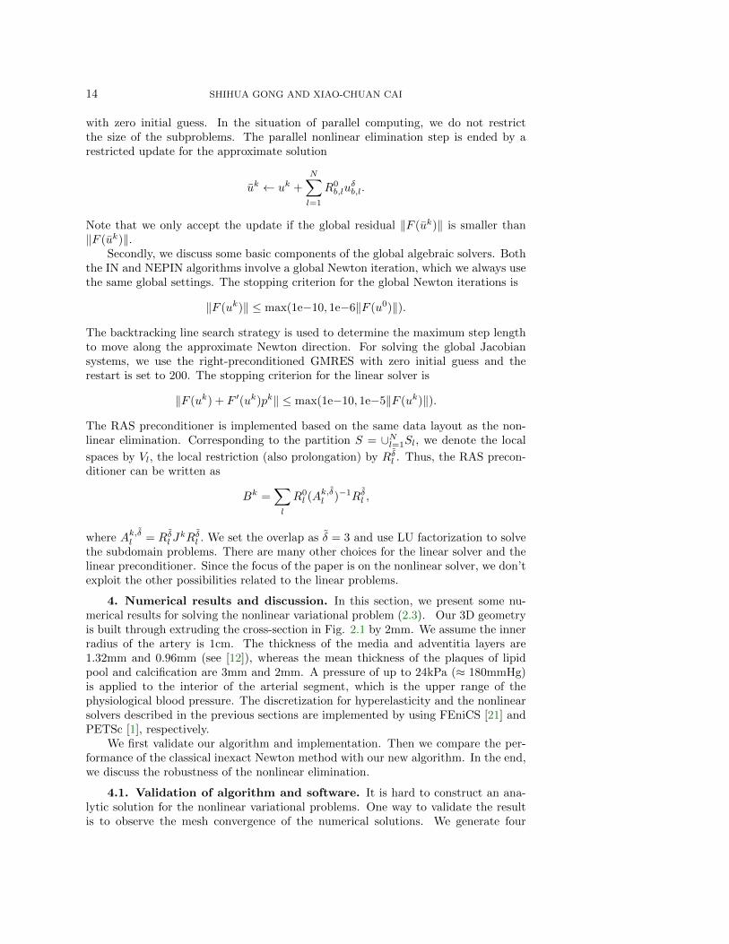
tetrahedral meshes for the arterial segment, denoting by M1, M2, M3, and M4. Thenumber of degrees of freedom defined on these meshes are 10080, 21693, 101046 and653601, respectively. Because of the curved boundary of the artery, the domains oc-cupied by these meshes are a little bit different. We plot the numerical solutions ofdisplacement in Fig. 4.1 for the case of the simple boundary load and the von Misesstresses in Fig. 4.2 for the case of follower boundary load. The deformation driven bythe simple pressure load is bigger than that driven by the follower pressure load, buttheir distributions and the stresses are similar.
Fig. 4.1: Numerical solutions of the displacement corresponding to meshes M1, M2,M3, M4 from left to right (simple boundary load)
Fig. 4.2: von Mises stresses on the deformed configurations corresponding to meshesM1, M2, M3, M4 from left to right (follower boundary load)
stands for the difference of numerical solutions obtained by IN and NEPIN.
We compute the difference of the numerical solutions obtained by IN and NEPIN,see Table 4.1. They are almost identical. We also consider the actual measurementsof the solution error by taking the numerical solution on the finest mesh as a referencesolution and interpolating the coarse-level solutions into the finest mesh. Table 4.1
16 SHIHUA GONG AND XIAO-CHUAN CAI
lists the errors in L2 and H1 norms. We denote by uhi as the numerical solution onMi driven by the simple pressure load, and uhi for that driven by the follower pressure
load. We also denote the nodal interpolation operator by Ihjhi
, which prolongates thenumerical solutions from Mi to Mj . Note that some nodal values are computed viaextrapolation since these nodes of the fine mesh are outside the domain occupied bythe coarse mesh. We can not compute the convergence orders since the meshes arenot quasi-uniform. But it is still clear that the computed solutions converge as themesh size goes to zero.
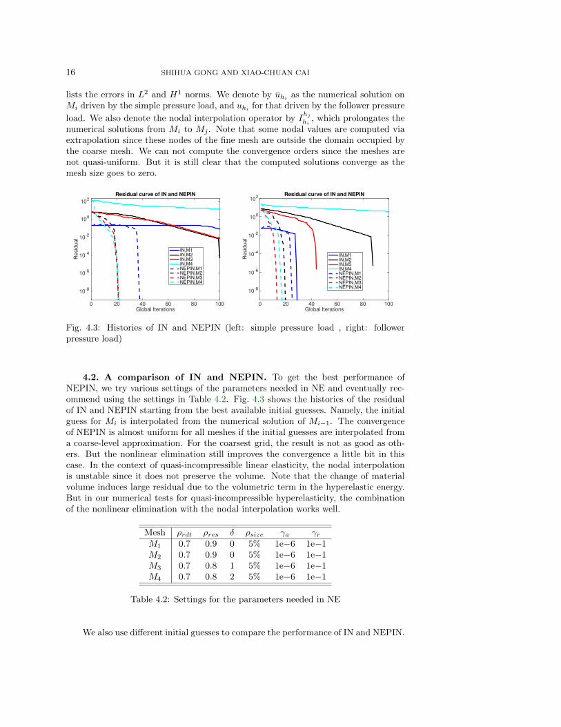
Fig. 4.3: Histories of IN and NEPIN (left: simple pressure load , right: followerpressure load)
4.2. A comparison of IN and NEPIN. To get the best performance ofNEPIN, we try various settings of the parameters needed in NE and eventually rec-ommend using the settings in Table 4.2. Fig. 4.3 shows the histories of the residualof IN and NEPIN starting from the best available initial guesses. Namely, the initialguess for Mi is interpolated from the numerical solution of Mi−1. The convergenceof NEPIN is almost uniform for all meshes if the initial guesses are interpolated froma coarse-level approximation. For the coarsest grid, the result is not as good as oth-ers. But the nonlinear elimination still improves the convergence a little bit in thiscase. In the context of quasi-incompressible linear elasticity, the nodal interpolationis unstable since it does not preserve the volume. Note that the change of materialvolume induces large residual due to the volumetric term in the hyperelastic energy.But in our numerical tests for quasi-incompressible hyperelasticity, the combinationof the nonlinear elimination with the nodal interpolation works well.
Table 4.2: Settings for the parameters needed in NE
We also use different initial guesses to compare the performance of IN and NEPIN.
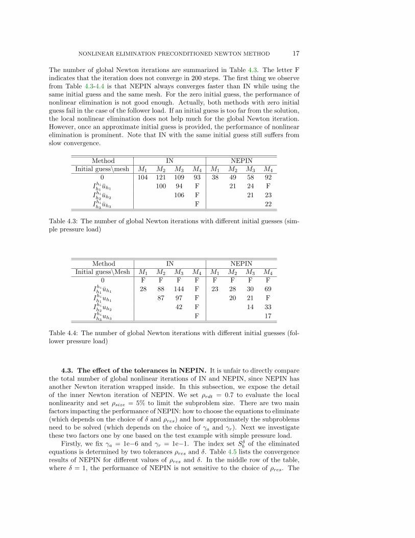
NONLINEAR ELIMINATION PRECONDITIONED NEWTON METHOD 17
The number of global Newton iterations are summarized in Table 4.3. The letter Findicates that the iteration does not converge in 200 steps. The first thing we observefrom Table 4.3-4.4 is that NEPIN always converges faster than IN while using thesame initial guess and the same mesh. For the zero initial guess, the performance ofnonlinear elimination is not good enough. Actually, both methods with zero initialguess fail in the case of the follower load. If an initial guess is too far from the solution,the local nonlinear elimination does not help much for the global Newton iteration.However, once an approximate initial guess is provided, the performance of nonlinearelimination is prominent. Note that IN with the same initial guess still suffers fromslow convergence.
Table 4.4: The number of global Newton iterations with different initial guesses (fol-lower pressure load)
4.3. The effect of the tolerances in NEPIN. It is unfair to directly comparethe total number of global nonlinear iterations of IN and NEPIN, since NEPIN hasanother Newton iteration wrapped inside. In this subsection, we expose the detailof the inner Newton iteration of NEPIN. We set ρrdt = 0.7 to evaluate the localnonlinearity and set ρsize = 5% to limit the subproblem size. There are two mainfactors impacting the performance of NEPIN: how to choose the equations to eliminate(which depends on the choice of δ and ρres) and how approximately the subproblemsneed to be solved (which depends on the choice of γa and γr). Next we investigatethese two factors one by one based on the test example with simple pressure load.
Firstly, we fix γa = 1e−6 and γr = 1e−1. The index set Sδb of the eliminatedequations is determined by two tolerances ρres and δ. Table 4.5 lists the convergenceresults of NEPIN for different values of ρres and δ. In the middle row of the table,where δ = 1, the performance of NEPIN is not sensitive to the choice of ρres. The
18 SHIHUA GONG AND XIAO-CHUAN CAI
Mesh M2 M3 M4
δ \ρres 0.7 0.8 0.9 0.7 0.8 0.9 0.7 0.8 0.9
0GN 25 23 21 30 34 47 31 52 50
ANE 2110
2214
2517
6817
5729
7742
6026
11847
10845
pct. 3.9% 4.4% 3.0% 3.3% 4.3% 0.8% 0.8% 0.5% 0.2%
1GN 25 32 30 24 21 26 24 28 34
ANE 425
304
7110
9912
13312
10821
11916
13522
17526
pct. 4.9% 4.9% 4.9% 4.0% 4.1% 4.1% 3.6% 1.9% 0.6%
2GN 100 69 56 29 30 22 26 21 30
ANE 00
81
503
16113
13112
11712
11012
12814
19923
pct. 0% 4.5% 4.9% 4.4% 3.6% 4.8% 3.0% 2.7% 1.2%
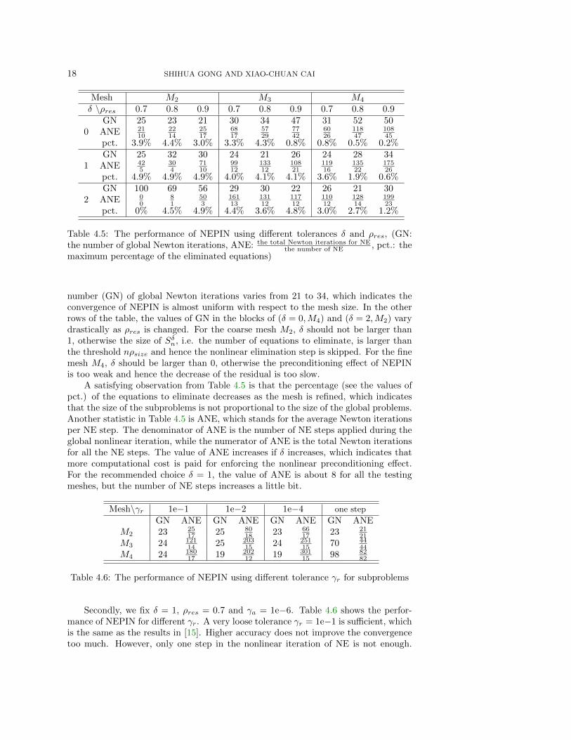
Table 4.5: The performance of NEPIN using different tolerances δ and ρres, (GN:the number of global Newton iterations, ANE: the total Newton iterations for NE
the number of NE , pct.: themaximum percentage of the eliminated equations)
number (GN) of global Newton iterations varies from 21 to 34, which indicates theconvergence of NEPIN is almost uniform with respect to the mesh size. In the otherrows of the table, the values of GN in the blocks of (δ = 0,M4) and (δ = 2,M2) varydrastically as ρres is changed. For the coarse mesh M2, δ should not be larger than1, otherwise the size of Sδn, i.e. the number of equations to eliminate, is larger thanthe threshold nρsize and hence the nonlinear elimination step is skipped. For the finemesh M4, δ should be larger than 0, otherwise the preconditioning effect of NEPINis too weak and hence the decrease of the residual is too slow.
A satisfying observation from Table 4.5 is that the percentage (see the values ofpct.) of the equations to eliminate decreases as the mesh is refined, which indicatesthat the size of the subproblems is not proportional to the size of the global problems.Another statistic in Table 4.5 is ANE, which stands for the average Newton iterationsper NE step. The denominator of ANE is the number of NE steps applied during theglobal nonlinear iteration, while the numerator of ANE is the total Newton iterationsfor all the NE steps. The value of ANE increases if δ increases, which indicates thatmore computational cost is paid for enforcing the nonlinear preconditioning effect.For the recommended choice δ = 1, the value of ANE is about 8 for all the testingmeshes, but the number of NE steps increases a little bit.
Mesh\γr 1e−1 1e−2 1e−4 one step
GN ANE GN ANE GN ANE GN ANEM2 23 25
17 25 8018 23 66
17 23 2121
M3 24 12114 25 203
15 24 25115 70 44
44M4 24 180
17 19 20212 19 301
15 98 8282
Table 4.6: The performance of NEPIN using different tolerance γr for subproblems
Secondly, we fix δ = 1, ρres = 0.7 and γa = 1e−6. Table 4.6 shows the perfor-mance of NEPIN for different γr. A very loose tolerance γr = 1e−1 is sufficient, whichis the same as the results in [15]. Higher accuracy does not improve the convergencetoo much. However, only one step in the nonlinear iteration of NE is not enough.
NONLINEAR ELIMINATION PRECONDITIONED NEWTON METHOD 19
Note that it is always the relative tolerance γr that stops the nonlinear iteration ofNE. If the residual is of magnitude γa = 1e−6, the quadratic convergence of New-ton’s method is observed for our test examples. That is why we do not expose theperformance of NEPIN for different γa.
5. Conclusions. The main contribution of this paper is to present a detailedanalysis of the preconditioning effect of nonlinear elimination and to apply the pro-posed method to 3D heterogeneous hyperelastic problems. In theory, we prove thatthe exact nonlinear elimination is able to reduce the residual and the local Lipschitzconstant of the nonlinear function and hence accelerates the convergence of Newtonmethod. For numerical computation, we propose a robust strategy to detect theequations causing the nonlinear stagnation. We also find two effective tricks to easethe thrashing phenomenon of nonlinear elimination: using an initial guess interpo-lated from a coarse level solution and extending the eliminating index set by addingthe neighboring d.o.f.. In future work, we will consider other arterial wall problemswith patient-specific geometry and the parallel performance of the algorithm.
REFERENCES
[1] S. Balay, S. Abhyankar, M. F. Adams, J. Brown, P. Brune, K. Buschelman, L. Dalcin,V. Eijkhout, W. D. Gropp, D. Kaushik, M. G. Knepley, L. C. McInnes, K. Rupp,B. F. Smith, S. Zampini, H. Zhang, and H. Zhang, PETSc users manual, Tech. ReportANL-95/11 - Revision 3.7, Argonne National Laboratory, 2018.
[2] J. M. Ball, Convexity conditions and existence theorems in nonlinear elasticity, Arch. forRation. Mech. Analysis, 63 (1976), pp. 337–403.
[3] D. Balzani, S. Deparis, S. Fausten, D. Forti, A. Heinlein, A. Klawonn, A. Quarteroni,O. Rheinbach, and J. Schroder, Numerical modeling of fluid–structure interaction in ar-teries with anisotropic polyconvex hyperelastic and anisotropic viscoelastic material modelsat finite strains, Int. J. Num. Methods Biomed. Eng., (2015).
[4] D. Balzani, P. Neff, J. Schroder, and G. A. Holzapfel, A polyconvex framework forsoft biological tissues. Adjustment to experimental data, Int. J. Solids Struct., 43 (2006),pp. 6052–6070.
[5] Y. Bazilevs, K. Takizawa, and T. E. Tezduyar, Computational Fluid-structure Interaction:Methods and Applications, John Wiley & Sons, 2013.
[6] D. Brands, A. Klawonn, O. Rheinbach, and J. Schroder, Modelling and convergencein arterial wall simulations using a parallel FETI solution strategy, Comput. MethodsBiomech. Biomed. Eng., 11 (2008), pp. 569–583.
[7] X.-C. Cai and D. E. Keyes, Nonlinearly preconditioned inexact newton algorithms, SIAM J.Sci. Comput., 24 (2002), pp. 183–200.
[8] X.-C. Cai and X. Li, Inexact Newton methods with restricted additive Schwarz based nonlinearelimination for problems with high local nonlinearity, SIAM J. Sci. Comput., 33 (2011),pp. 746–762.
[9] R. S. Dembo, S. C. Eisenstat, and T. Steihaug, Inexact Newton methods, SIAM J. Num.Anal. 19 (1982), pp. 400–408.
[10] P. Deuflhard, Newton Methods for Nonlinear Problems: Affine Invariance and AdaptiveAlgorithms, vol. 35, Springer Science & Business Media, 2011.
[11] S. C. Eisenstat and H. F. Walker, Globally convergent inexact Newton methods, SIAM J.Optim., 4 (1994), pp. 393–422.
[12] G. A. Holzapfel, Determination of material models for arterial walls from uniaxial extensiontests and histological structure, J. theoretical Bio., 238 (2006), pp. 290–302.
[13] G. A. Holzapfel, T. C. Gasser, and R. W. Ogden, A new constitutive framework for arterialwall mechanics and a comparative study of material models, J. Elasticity, 61 (2000), pp. 1–48.
[14] J. Huang, C. Yang, and X.-C. Cai, A nonlinearly preconditioned inexact Newton algorithmfor steady state lattice Boltzmann equations, SIAM J. Sci. Comput., 38 (2016), pp. A1701–A1724.
[15] F.-N. Hwang, Y.-C. Su, and X.-C. Cai, A parallel adaptive nonlinear elimination precondi-tioned inexact Newton method for transonic full potential equation, Computers & Fluids,
20 SHIHUA GONG AND XIAO-CHUAN CAI
110 (2015), pp. 96–107.[16] A. Klawonn, M. Lanser, and O. Rheinbach, Nonlinear FETI-DP and BDDC methods,
SIAM J. Sci. Comput., 36 (2014), pp. A737–A765.[17] A. Klawonn, M. Lanser, and O. Rheinbach, Toward extremely scalable nonlinear domain
decomposition methods for elliptic partial differential equations, SIAM J. Sci. Comput., 37(2015), pp. C667–C696.
[18] A. Klawonn, M. Lanser, O. Rheinbach, and M. Uran, Nonlinear FETI-DP and BDDCmethods: a unified framework and parallel results, SIAM J. Sci. Comput., 39 (2017),pp. C417–C451.
[19] P. Ciarlet, Mathematical Elasticity, Vol. I : Three-Dimensional Elasticity, Series “Studiesin Mathematics and its Applications”, North-Holland, Amsterdam, 1988.
[20] P. J. Lanzkron, D. J. Rose, and J. T. Wilkes, An analysis of approximate nonlinear elim-ination, SIAM J. Sci. Comput., 17 (1996), pp. 538–559.
[21] A. Logg, K.-A. Mardal, and G. Wells, Automated Solution of Differential Equations by theFinite Element Method: The FEniCS Book, vol. 84, Springer Science & Business Media,2012.
[22] J. Schroder and P. Neff, Invariant formulation of hyperelastic transverse isotropy based onpolyconvex free energy functions, Int. J. Solids Struct., 40 (2003), pp. 401–445.


![Constraint-Preconditioned Inexact Newton Method for ... · PDF filespace Newton method for hydraulic analysis of water distribution networks. ... gradient (CG) method to ... [14].](https://static.documents.pub/doc/80x56/5aa8d4947f8b9a72188c189f/constraint-preconditioned-inexact-newton-method-for-newton-method-for-hydraulic.jpg)


