HAL Id: hal-01515958 https://hal-enpc.archives-ouvertes.fr/hal-01515958 Submitted on 28 Apr 2017 HAL is a multi-disciplinary open access archive for the deposit and dissemination of sci- entific research documents, whether they are pub- lished or not. The documents may come from teaching and research institutions in France or abroad, or from public or private research centers. L’archive ouverte pluridisciplinaire HAL, est destinée au dépôt et à la diffusion de documents scientifiques de niveau recherche, publiés ou non, émanant des établissements d’enseignement et de recherche français ou étrangers, des laboratoires publics ou privés. A novel method for determining the small-strain shear modulus of soil using the bender elements technique Yejiao Wang, Nadia Benahmed, Yu-Jun Cui, Anh Minh Tang To cite this version: Yejiao Wang, Nadia Benahmed, Yu-Jun Cui, Anh Minh Tang. A novel method for determining the small-strain shear modulus of soil using the bender elements technique. Canadian Geotechnical Journal, NRC Research Press, In press, 54 (2), pp.280-289. 10.1139/cgj-2016-0341. hal-01515958
Transcript
HAL Id: hal-01515958https://hal-enpc.archives-ouvertes.fr/hal-01515958
Submitted on 28 Apr 2017
HAL is a multi-disciplinary open accessarchive for the deposit and dissemination of sci-entific research documents, whether they are pub-lished or not. The documents may come fromteaching and research institutions in France orabroad, or from public or private research centers.
L’archive ouverte pluridisciplinaire HAL, estdestinée au dépôt et à la diffusion de documentsscientifiques de niveau recherche, publiés ou non,émanant des établissements d’enseignement et derecherche français ou étrangers, des laboratoirespublics ou privés.
A novel method for determining the small-strain shearmodulus of soil using the bender elements technique
Yejiao Wang, Nadia Benahmed, Yu-Jun Cui, Anh Minh Tang
To cite this version:Yejiao Wang, Nadia Benahmed, Yu-Jun Cui, Anh Minh Tang. A novel method for determiningthe small-strain shear modulus of soil using the bender elements technique. Canadian GeotechnicalJournal, NRC Research Press, In press, 54 (2), pp.280-289. �10.1139/cgj-2016-0341�. �hal-01515958�
The small-strain shear modulus (Gmax) is a parameter of paramount importance in describing 42
the elastic properties of soil. It is widely used in the analysis of dynamic problems in 43
anti-seismic engineering (Zhou et al. 2005; Yang et al. 2009; Luke et al. 2013). It is also used 44
to assess the soil stiffness in geo-environmental engineering (Tang et al. 2011; Gu et al. 2013; 45
Hoyos et al. 2015). The value of Gmax is usually determined from shear wave velocity (Vs) 46
measurements either in the field or in the laboratory. 47
The measurement of Vs can be obtained from conventional laboratory experiments using 48
resonant column (Hardin and Richart 1963; Anderson and Stokoe 1978; Fam et al. 2002), 49
torsional shear tests (Iwasaki et al. 1978; Youn et al. 2008), flat transducers and 50
accelerometers (Brignoli et al. 1996; Mulmi et al. 2008; Wicaksono et al. 2008) and 51
piezoelectric bender elements technique (Dyvik and Madshus 1985; Viggiani and Atkinson 52
1995; Brignoli et al. 1996; Jovičić et al. 1996; Pennington et al. 2001; Lings and Greening 53
2001; Leong et al. 2005; Yamashita et al. 2009; Clayton 2011). The bender elements 54
technique was first introduced by Shirley and Hampton (1978) and Shirley (1978) to soil 55
testing, and due to its ability to measure the shear wave velocity of soil in a small-strain range, 56
less than 0.001%, and in a wide range of stress conditions, it has taken a lot of interest of 57
researchers. Nowadays, the bender elements transducers have been becoming a common 58
laboratory tool, and have been incorporated in many geotechnical testing devices, such as 59
oedometers (Dyvik and Olsen 1991; Zeng and Grolewski 2005; Sukolrat 2007), cubical and 60
conventional triaxial apparatuses (Gajo et al. 1997; Jovičić and Coop 1998; Kuwano et al. 61
1999; Pennington et al. 2001; Fioravante and Capoferri 2001; Sukolrat et al. 2006; Leong et 62
4
al. 2009; Finno and Cho 2011; Aris et al. 2012; Styler and Howie 2013), resonant column 63
apparatuses (Ferreira et al. 2007; Youn et al. 2008; Gu et al. 2013). 64
Despite the popularity of its use, difficulties of signal interpretation of bender elements 65
technique, mainly in the determination of the wave arrival time, are still remaining. Different 66
methods and frameworks for the signal interpretation were reported (Lee and Santamarina 67
2005; Viana da Fonseca et al. 2009; Leong et al. 2009; Arroyo et al. 2010), but none has been 68
widely accepted as a standard. In fact, the complex phenomena of wave propagation in a soil 69
sample have not been clearly understood yet, which represents an obstacle to the 70
determination of the arrival point accurately and objectively (Camacho-Tauta et al. 2013). 71
In the field of geotechnical engineering, most tested materials with bender elements are soils 72
with low stiffness, and generally, the chosen frequency of excitation voltage in most studies 73
ranges from 1 to 30 kHz (Lee and Santamarina 2005; Sukolrat 2007; Youn et al. 2008; Viana 74
da Fonseca et al. 2009; Leong et al. 2009). A few researchers used the bender elements 75
technique for stiffer materials, including sandstones (Alvarado 2007), cement treated clay 76
(Hird and Chan 2008), and argillaceous rocks (Arroyo et al. 2010). In these cases, the 77
working frequency range is different, and higher input frequency should be chosen due to the 78
higher resonant frequency of stiff material (Lee and Santamarina 2005). 79
This technical note puts forward an objective method for the signal interpretation of bender 80
elements technique, with respect to the determination of the first arrival time of shear wave. 81
This method is based on the comparison of both S-wave and P-wave received signals 82
obtained on the same sample with a single pair of bender elements to determine a unique 83
arrival point. In this study, the bender elements tests were performed on compacted 84
5
lime-treated silt samples extending, thus, this technique to stiff soils. The results obtained by 85
the proposed method are validated by comparing with those of other methods. 86
87
Background 88
Working principal of Bender Elements 89
The bender elements are piezo-electrical transducers, which consist of two thin piezo-ceramic 90
bimorph sheets with external conducting surfaces, mounted together with a conductive metal 91
shim at the centre. Details of the connection are given in Figure 1a. When an input waveform 92
voltage is applied on the S-wave transmitter, one piezoceramic sheet extends and the other 93
contracts, leading the transmitter to bend and generate a shear wave signal. The S-wave 94
receiver bends when the shear wave arrives, propagating an electrical signal that can be 95
visualised and measured by a digital oscilloscope. The operation of bender elements for 96
S-wave transmission was well described by other researchers (Dyvik and Madshus 1985; 97
Lings and Greening 2001; Lee and Santamarina 2005; Camacho Tauta et al. 2012). 98
Lings and Greening (2001) introduced a bender-extender element to transmit and receive 99
both S-wave and P-wave with a single pair of transducers. The bender (or S-wave) receiver 100
and transmitter in bender element testing also act as an extender (or P-wave) transmitter and 101
receiver, respectively. Specifically, when an input voltage is applied on the extender 102
transmitter, both two piezoceramic sheets with opposite polarisations extend or contract at the 103
same time, causing the propagation of P-wave in a longitudinal direction. The P-wave wiring 104
and transmitting are illustrated in Figure 1b. Note that the measurement of P-wave velocity is 105
6
mainly useful for unsaturated soils. Since in the saturated soils, P-wave usually travels much 106
faster through water than through soil skeletion (Leong et al. 2009). Nevertheless, in this 107
study, the degree of saturation of the tested material is lower than 95%. Bardet and Sayed 108
(1993) who studied the Ottawa sand reported that the P-wave velocity became close to the 109
value of dry sample when the degree of saturation decreased from 100% to 95%. 110
Determination of shear wave velocity 111
During bender elements testing, both the transmitted and received signals are recorded to 112
determine the travel time, t, of S-wave through a sample. The shear wave velocity, Vs, can 113
then be calculated from the tip-to-tip travel length between the bender elements, Ltt, and 114
travel time, t, as follows (Viggiani and Atkinson, 1995): 115
tLV tt
s = (1) 116
According to the theory of shear wave propagation in an elastic body, the small strain shear 117
modulus, Gmax, can be determined by the following formula: 118
2max sVG ρ= (2) 119
where ρ is the density of soil sample. 120
Interpretation of bender element tests usually takes the advantage of the knowledge and 121
experience gained into the development of in situ geophysical tests such as Down-Hole and 122
Cross-Hole tests or even surface tests such as SASW tests (Stokoe et al. 2004; Viana da 123
Fonseca et al. 2006). 124
Determination of travel time 125
An accurate determination of the travel time is a crucial issue to get a reliable value of Vs, 126
7
hence Gmax. The existing common methods for determining travel time can be classified into 127
two categories: time domain and frequency domain methods. 128
The time domain methods determine the travel time directly from the time lag between the 129
transmitted and received signals. Referring to different characteristic points, the time domain 130
methods can be divided into “arrival-to-arrival” method, “peak-to-peak” method and “cross 131
correlation method”. 132
The first method, based on the visual inspection of the received signal, is the most commonly 133
used one; however, the determination of an accurate arrival point using this method is still 134
controversial and quite subjective due to the complex received signal, wave’s reflexion and 135
the near field effect. Many studies reported that the near field effect decreases with the 136
increase of frequency or the ratio of the wave path length to wavelength, Ltt/λ. Arulnathan et 137
al. (1998) reported that the near field effect disappears when this ratio is larger than 1. 138
Pennington et al. (2001) pointed out that when the Ltt/λ values range from 2 to 10, a good 139
signal can be obtained. Wang et al. (2007) advocated a ratio greater than or equal to 2 to 140
avoid the near field effect. Similarly, a value of 3.33 was recommended by Leong et al. (2005) 141
to improve the signal interpretation. 142
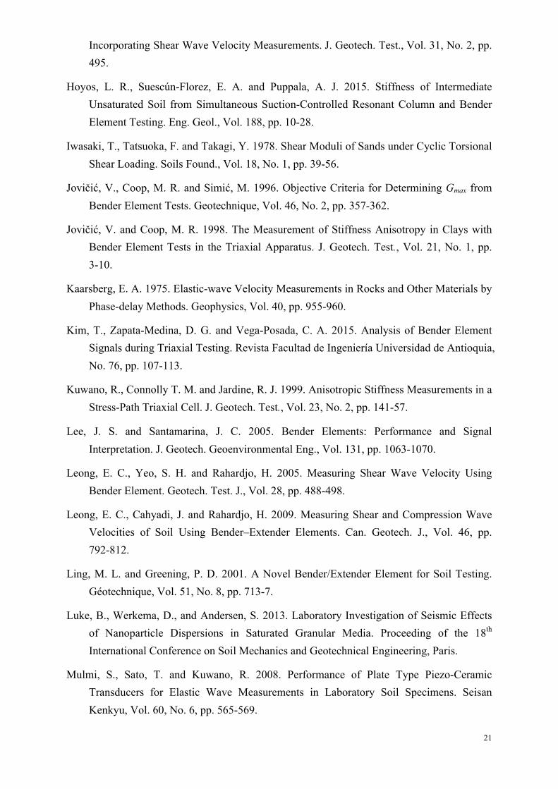
Figure 2 shows a typical single sinusoidal S-wave transmitted signal and its corresponding 143
received signal. Generally, point “a” (the first deflection) is taken as the arrival of the near 144
field component of received signal (Brignoli et al. 1996). Both point “b” (the first reversal) 145
and point “c” (zero after first reversal) are chosen as the arrival points of S-wave by most 146
researchers (Brignoli et al. 1996; Lee and Santamarina 2005; Youn et al. 2008; Yamashita et 147
al. 2009; Arroyo et al. 2010). 148
8
The “peak-to-peak” method is also widely applied in the signal interpretation. In this method, 149
time delay between the peak of transmitted signal and the first major peak of received signal 150
(point “d” in Figure 2) is regarded as the travel time (Clayton et al. 2004; Ogino et al. 2015). 151
Note that, since the frequency of received signal may be slightly different from that of 152
transmitted signal, and that the nature of the soil and size of the sample often affect the shape 153
of the signal which could present more than one peak, great attention should be paid to the 154
calculation of travel time by the “peak-to-peak” method. 155
“Cross-correlation” method is another kind of time domain method. It assumes the travel time 156
as the time shift corresponding to the peak value of cross-correlation function between the 157
transmitted and received signals. The cross-correlation approach, first adopted by Viggiani 158
and Atkinson (1995), is based on the following expression:: 159
( ) ( )dttytxT
CCT
Txy ττ += ∫→∞ 0
*1lim)( (3) 160
where x(t) and y(t) are the received and transmitted signals respectively, T is the time record 161
and τ is the time shift between two signals. First, the transmitted and received signals are 162
converted to their linear spectrums using Fast Fourier Transform. Then the cross-power 163
spectrum can be built based on the linear spectrum of received signal and the complex 164
conjugate of the linear spectrum of transmitted signal. Eventually, the maximum of the 165
cross-correlation function gives the travel time of shear wave. However, the accuracy of the 166
cross-correlation method is largely dependent on the quality of received signals. Many 167
limitations due to complex characteristics of received signal or incompatible transformation 168
have been reported by several researchers (Arulnathan et al. 1998; Viana da Fonseca et al. 169
2009; Chan 2012). 170
9
Frequency domain methods estimate the travel time according to the relationship between the 171
change in the phase angle, which corresponds to the phase shift between the transmitter and 172
receiver signals, and input frequency (Greening and Nash 2004; Viana da Fonseca et al. 2009; 173
Ogino et al. 2015). These methods can be applied using discrete method called “π-point” 174
method (Greening and Nash 2004; Viana da Fonseca et al. 2009), or continuous method such 175
as Frequency Spectral Analysis (Greening and Nash 2004; Viana da Fonseca et al. 2009; Kim 176
et al. 2015). They were first performed on rock and mud samples by Kaarberg (1975) and 177
later widely accepted by other researchers (Greening et al. 2003; Gutierrez 2007; Viana da 178
Fonseca et al. 2009), thanks to their negligible effect of extraneous signals. 179
In the “π-point” method, a continuous sinusoidal wave at a single frequency is used as an 180
input signal, the continuous sinuous wave transmitter and receiver are displayed in an X-Y 181
plot on an oscilloscope, and the phase shift between these two signals is measured. The 182
frequency of transmitter is increased very slightly from a low value, inducing a phase shift 183
between the two signals. When these signals are in phase or out of phase, i.e. the phase 184
differences are multiple N of π or (-π), the corresponding frequency, f, and the number of 185
wavelength, N, are recorded. 186
It is well known that velocity, V, can be determined from the wavelength, λ, and the 187
frequency (Viana da Fonseca et al. 2009): 188
NLffV == λ (4) 189
where the travel time, t, can be deduced from: 190
fNt = (5) 191
10
This indicates that the slope of the N-f plot represents the travel time. 192
Result given by this method is more objective than that obtained by time domain method. 193
However, it has the drawbacks of time consuming and limited interpretable points (Viana da 194
Fonseca et al. 2009). 195
Compared with the time-consuming “π-point” method, continuous method (Frequency 196
Spectral Analysis) provides more available information in a short period of time with less 197
effort. Continuous method applies a sweep signal which has a wide frequency spectrum (for 198
example: 0 – 20 kHz) as input wave and uses a spectrum analyzer to establish the relationship 199
between the frequency and the phase change, as introduced by Greening et al. (2003), 200
Greening and Nash (2004) and explained in details by Kim et al. (2015). Specifically, the 201
spectrum analyzer computes the coherence function between the transmitted and received 202
signals. Based on the coherence function and phase angle it provides, the travel time can be 203
determined directly from the slope of the linear line representing the relationship between the 204
frequency and phase angle. However, further analysis is necessary when applying this 205
method if the result convergence cannot be reached quickly (Viana da Fonseca et al. 2009). 206
Viana da Fonseca et al. (2009) also proposed a practical framework which combines both 207
time-domain and frequency-domain methods for an enhanced interpretation of the bender 208
element testing results. Nevertheless, the differences of the travel time determined by the time 209
domain method and frequency domain method are quite large, and the causes are still not 210
well understood (Greening et al. 2003; Greening and Nash 2004; Viana da Fonseca et al. 211
2009; Ogino et al. 2015). Therefore, there is still a strong need of searching a simple and 212
objective approach for the bender element testing interpretation with a reliable determination 213
11
of the arrival time. 214
In this study, the “arrival-to-arrival” method, “peak-to-peak” method, and “π-point” method 215
are evaluated through the interpretation of signals obtained on compacted lime treated soils. 216
Furthermore, based on the observation that the S-wave received signal presents an identical 217
travel time and opposite polarity compared with that of the S-wave components in P-wave 218
received signal, especially at high frequency, a novel method namely S+P method is 219
proposed and its accuracy is proved by the comparison with “π-point” method. 220
221
Experimental methods 222
Tested Material 223
The soil used in this study was a plastic silt, taken from an experimental embankment with 224
the ANR project TerDOUEST (Terrassements Durables - Ouvrages en Sols Traités, 2008 - 225
2012) at Héricourt, France. This soil was first air-dried, ground and sieved to 0.4 mm. 226
Quicklime was used in the treatment. The soil powder was first mixed thoroughly with 2% 227
lime, and then humidified to reach two target water contents (at dry or wet side of optimum). 228
More details about the geotechnical properties of this silt and the preparation process of 229
samples can be found in Wang et al. (2015). In this study, four compacted lime-treated 230
samples (50 mm in diameter and 50 mm in height) with degree of saturation, Sr = 72 % at dry 231
side and Sr = 93 % at wet side, were tested. The specific sample information is listed in Table 232
1. 233
Experimental Techniques 234
12
The bender element system used in this study consists of two bender elements (one S-wave 235
transmitter/P-wave receiver and one S-wave receiver/P-wave transmitter, as shown in Figure 236
3), installed at the two extremities of the soil sample. Beforehand, a slot was carried out on 237
the surface of each sample extremity with the same direction to facilitate the insertion of the 238
protruded part of the bender elements, and a good alignment of the latter. Afterwards, the 239
sample (50 mm in diameter and 50 mm in height) was placed on a home-made wooden 240
sample holder (see Figure 4a) specially designed to forbid any wave transmission outside the 241
soil sample, which may interfere with the signal arrival (Brignoli et al. 1996; Lee and 242
Santamarina 2005). Additional force was provided by the holder to enhance a good contact 243
between the benders and the sample. Special care was taken to avoid any cross-talk by 244
improving the shielding and grounding of the system. The output signal (± 20V sine pulse) 245
was generated by a function generator (TTi TG1010A) and amplified by a power amplifier. 246
Both the transmitter and the receiver signals were captured with an oscilloscope (Agilent 247
DSO-X 2004A). The set-up of the system used is presented in Figure 4a and details of the 248
arrangement of devices are illustrated in Figure 4b. All the four different interpretation 249
methods presented previously (“arrival-to-arrival”, “peak-to-peak”, “π-point” and S+P 250
methods) were applied for each sample. As for the conventional “arrival-to-arrival” and 251
“peak-to-peak” methods, a single pulse S-wave with various input frequency was used as 252
transmitted signal. In S+P method, both S-wave and P-wave signals transmitted through the 253
same sample by modifying the connection between the two benders, as illustrated in Figure 254
4b. A continuous sweep signal (frequency increased slowly from 20 kHz to 50 kHz) was 255
applied in the “π-point” method. 256
13
Prior to testing, calibration of bender elements (tip-to-tip calibration) was carried out by 257
holding the two benders (transmitter and receiver) in contact with each other directly without 258
sample. Both S-wave transmitter and P-wave transmitter were generated to measure the delay 259
times for these two transmitters (td_S = 5.5 µs and td_P = 3.5 µs). These delay times were 260
accounted for in the calculation of travel time when applying the time domain method. 261
262
Experimental Results 263
Figure 5 presents the results of sample D1 with the time domain methods (conventional 264
arrival-to-arrival method and peak-to-peak method). The S-wave transmitted signals with 265
various frequencies are considered (dashed lines) and the S-wave received signals are 266
presented in solid lines. In the arrival-to-arrival method, the first reversal in the received 267
signal is chosen as the arrival point of S-wave. Besides, the first major peak is highlighted to 268
calculate the time delay by the peak-to-peak method. It is observed that for the relatively low 269
frequencies used here (f = 5, 10 and 15 kHz), the interpretation of these received signals is 270
ambiguous because of the evident near field effect. However, the signals at higher 271
frequencies, from 20 kHz to 50 kHz, become quite clear and the near field less marked. These 272
cases correspond to a ratio of wave path length to wavelength, Ltt/λ, larger than or equal to 1.9, 273
and are in good agreement with those reported in the literature (Sanchez-Salinero et al. 1986; 274
Brignoli et al. 1996; Arulnathan et al. 1998; Pennington et al. 2001; Leong et al. 2005; Wang 275
et al. 2007). The results obtained from the “π-point” method on the sample (w = 17%, with a 276
curing time, tc = 25 h) are shown in Figure 6. A good linear relationship between the number 277
of wavelength and frequency is obtained. The travel time, t, can be determined as 0.1441 ms 278
14
directly from the slope of the matched line, according to Equation 5. Additionally, the good 279
linear relationship observed also highlights that the frequency ranging from 25 to 50 kHz is 280
reasonable and suitable for the determination of shear wave velocity by the time domain 281
method. 282
In Figure 7, the S-wave and P-wave transmitted signals and the corresponding received 283
signals are gathered. The arrival point of S-wave received signal can be determined by 284
referring to P-wave received signal. It is well known that P-wave component travels the 285
fastest, thus arrives first before the S-wave received signal. Specifically, the arrival point of 286
S-wave received signal (point S) corresponds to the initial main excursion (point S_p), which 287
is in the opposite direction of movement compared to that of point S in the S-wave received 288
signal. Apparently, the curvature of these points (S and S_p) becomes much sharper when the 289
input frequency increases up to 40 or 50 kHz, as shown in Figure 7c and 7d. Furthermore, the 290
arrival point of P-wave received signal (point P) just corresponds to the arrival point of the 291
near field components (point P_s) in the S-wave received signal. This is in good agreement 292
with the observation by Brignoli et al. 1996 - a “near field component” travelling at a similar 293
velocity as P-wave was observed on a dry sample. Therefore, we propose this method, 294
namely S+P method to determine the arrival point of S-wave: the arrival time is defined by 295
point S (corresponding point S_p in the P-wave received signal). 296
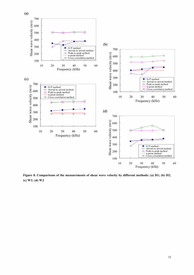
To verify the accuracy of this S+P method, Figure 8 collects all data of shear wave velocity 297
obtained from different interpretation methods. The results obtained from the S+P method are 298
compared with those from other methods. Note that in the arrival-to-arrival method, point b 299
(first reversal as mentioned above) is chosen as the arrival point of S-wave. As for the result 300
15
by π-point method in Figure 8, the straight line represents a unique value of travel time which 301
is determined as the input frequency slowly increasing from about 20 kHz to 50 kHz in each 302
case. The differences between the shear wave velocities (Vs) obtained from the conventional 303
time domain methods (arrival-to-arrival method and peak-to-peak method) and that from the 304
“π-point” method are about 30%. Similar ranges of difference are reported by other 305
researchers (Viggiani and Atkinson 1995; Viana da Fonseca et al. 2009; Ogino et al. 2015). 306
Nevertheless, the difference between the results obtained from S+P method and that taken 307
from “π-point” method is only around 10% in all tests; while this difference shows a good 308
agreement between the results obtained from S+P method and those from cross correlation 309
method, especially in the high frequency range, as illustrated in Figure 8. Therefore, the 310
accuracy of the proposed method (S+P method) can be confirmed. 311
312
Discussions 313
The results obtained in this study show that the S-wave received signals are unreadable at 314
lower frequencies (f = 5, 10 and 15 kHz), due to the influence of near field components. The 315
effect of the latter is usually significant insofar as it obscures the shear wave arrival time 316
point when the input frequency is low and the distance between the transmitter and receiver is 317
short. Many researchers used the ratio of wave path length to wavelength Ltt/λ as an essential 318
parameter to describe the near field effect. The near field effect can be reduced markedly with 319
the increase of Ltt/λ, by improving the input frequency of transmitter or enlarging the distance 320
between the transmitter and the receiver. 321
16
The results indicate also that the near field effect diminishes and a much clear received signal 322
appears as the Ltt/λ value reaches 1.91 (in the arrival-to-arrival method). Similar conclusion 323
can be made referring to the results of “π-point” method which shows a good linear 324
relationship between the number of wavelength and frequency when the input frequency 325
increases from 20 kHz (in case of Ltt/λ = 1.9). 326
A higher frequency makes the received signal more readable in case of testing on a stiff 327
material such as compacted lime-treated silt. However, the P-wave component can become 328
significant when the excitation frequency is high (Brignoli et al. 1996). This is different from 329
a near field component (Lee and Santamarina 2005). Bender element can also generate small 330
compressive displacements even though the main displacements produced are of shear nature 331
(Brignoli et al. 1996). More importantly, the small compressive components (P-wave 332
components) can be prominent in case of high frequency being excited on stiff materials, 333
resulting in slight interference with the shear components (S-wave components) which have 334
relatively slower travel velocity. Conversely, some shear displacements would be generated 335
simultaneously with the major excitation of compressive displacements. Note that the polarity 336
of S-wave components is always contrary to that of P-wave components in the same signal. It 337
is even important that the travel velocity of S-wave components in P-wave received signal is 338
identical with that of the S-wave received signals. 339
According to the analyses above, the determination of arrival point of S-wave received 340
signals becomes clear and objective using the S+P method. That is, based on the comparison 341
between S-wave and P-wave received signals, a unique point, S (as illustrated in Figure 7), 342
can be identified and it corresponds to the arrival point of S-wave. This point located in 343
17
S-wave received signal, corresponding exactly to the point S_p in P-wave received signal, 344
which shows opposite direction of movement in comparison with the point S in S-wave 345
signal. 346
The results from S+P method show a small effect of input frequency (in a range from 20 to 347
50 kHz) on the shear wave velocity. As Figure 8 shows, shear wave velocity increases 348
slightly as the input frequency increases. Similar phenomena were reported by other authors. 349
Youn et al. (2008) pointed out that the shear wave velocity obtained from time domain 350
method presents a small increasing trend with the increase of excitation frequency. Yamashita 351
et al. (2009) also noted that the shear modulus increases with the increase of excitation 352
frequency. To a certain extent, it might be a possible reason to explain why a slight 353
decreasing trend of arrival time is observed when the excitation frequency increases. 354
Specifically, when the frequency is relatively low (as shown in Figure 7a and 7b), point S 355
determined by S+P method as the arrival point is not very clear. By contrast, in the case of 356
high frequency (as shown in Figure 7c and 7d), point S is easy to be distinguished due to a 357
sharp curvature at point S_p in the P-wave received signal. Brignoli et al. (1996) also 358
recommended that high frequency should be used when measuring the P-wave components. 359
360
Conclusions 361
Due to the near field effect, reflected waves and soil properties, determining the shear wave 362
arrival time accurately and reliably in bender elements testing is difficult and still 363
controversial, and new methods need to be developed. 364
18
In this study, a novel method is proposed for a practical interpretation of the results from 365
bender element tests, for unsaturated or nearly saturated soil specimen. This method, namely 366
S+P method, is mainly based on the comparison between the S-wave and P-wave received 367
signals, and enables the determination of the arrival point of S-wave signal in a more 368
objective fashion. When a high frequency S-wave signal is excited, the P-wave components 369
become evident, and are easy to be distinguished from the S-wave received signal. Note that 370
the P-wave received signal also includes some S-wave components which arrive after the 371
P-wave components. Based on the identical travel velocity of S-wave components in both 372
S-wave received signal and P-wave received signal, and the opposite polarities between these 373
two different S-wave components, a unique arrival point of S-wave can be determined. 374
Comparisons between the results obtained by this method and those by the π-point method 375
and cross correlation method were made, indicating the relevance of the proposed method. It 376
is also worth noting that compared to the π-point method, the proposed method is less time 377
consuming. 378
19
Acknowledgements
The authors wish to thank the China Scholarship Council (CSC) and Ecole des Ponts
ParisTech for their financial supports. They also acknowledge the technical support provided
by IRSTEA Aix-en-Provence.
References
Alvarado, G. 2007. Influence of Late Cementation on the Behaviour of Reservoir Sands. Diss. PhD thesis, Imperial College London.
Anderson, D. G. and Stokoe, K. H. 1978. Shear Modulus: A Time-Dependent Soil Property. In: Dynamic Geotechnical Testing, ASTM International.
Arroyo, M., Pineda, J. A. and Romero, E. 2010. Shear Wave Measurements Using Bender Elements in Argillaceous Rocks. Geotech. Test. J., Vol. 33, pp. 1-11.
Arulnathan, R., Boulanger, R. W. and Riemer, M. F. 1998. Analysis of Bender Element Tests. Geotech. Test. J., Vol. 21, No. 2, pp. 120-131.
Aris M., Benahmed N. and Bonelli S. 2012. A Laboratory Study on the Behaviour of Granular Material Using Bender Elements. Euro. J. Environ. Civil. Engineer., Vol. 16, No. 1, pp. 97-110.
Bardet, J. P. and Sayed, H. 1993. Velocity and Attenuation of Compressional Waves in Nearly Saturated Soils. Soil Dyn. Earthq. Eng., Vol. 12, No. 7, pp. 391-401.
Brignoli, E. G. M., Gotti, M. and Stokoe, K. H. 1996. Measurement of Shear Waves in Laboratory Specimens by Means of Piezoelectric Transducers. Geotech. Test. J., Vol. 19, pp. 384-397.
Camacho-Tauta, J. F., Reyes-Ortiz, O. J. and Jimenez Alvarez, J. D. 2013. Comparison between Resonant-Column and Bender Element Tests on Three Types of Soils. Dyna, Vol. 80, No. 182, pp. 163-172.
Camacho-Tauta, J. F., Jimenez Alvarez, J. D. and Reyes-Ortiz, O. J. 2012 A Procedure to Calibrate and Perform Bender Element Test. Dyna, Vol. 79, No. 176, pp. 10-18,.
Chan, C. M. 2012. Variations of Shear Wave Arrival Time in Unconfined Soil Specimens Measured with Bender Elements. Geotech. Geo. Eng., Vol. 30, No. 2, pp. 461-468.
Clayton, C. R. I., Theron, M. and Best, A. I. 2004. The Measurement of Vertical Shear-Wave Velocity Using Side-Mounted Bender Elements in the Triaxial Apparatus. Géotechnique, Vol. 54, No. 7, pp. 495-498.
20
Clayton, C. R. I. 2011. Stiffness at Small Strain: Research and Practice. Géotechnique, Vol. 61, No. 1, pp. 5-37.
Dyvik, R. and Madshus, C. 1985. Lab Measurements of Gmax Using Bender Elements. Proceedings of the conference on the Advances in the Art of Testing Soil under Cyclic Conditions, New York: ASCE Geotechnical Engineering Division, pp. 186-196.
Dyvik, R. and Olsen, T. S.. 1991. Gmax Measured in Oedometer and DSS tests Using Bender Elements. Publikasjon-Norges Geotekniske Institutt, Vol. 181, pp. 1-4.
Fam, M. A., Cascante, G., and Dusseault, M. B. 2002. Large and Small Strain Properties of Sands Subjected to Local Void Increase. J. Geotech. Geoenviron., ASCE, Vol. 128, No. 12, pp. 1018-1025.
Ferreira, C., Viana da Fonseca, A. and Santos. J. A. 2007. Comparison of Simultaneous Bender Element Test and Resonant Column Tests on Porto Residual Soils. Soil Stress-Strain Behavior: Measurement, Modeling and Analysis, Springer Netherlands, pp. 523-535.
Finno, R. and Cho, W. 2011. Recent Stress-History Effects on Compressible Chicago Glacial Clays. J. Geotech. Geoenviron. Eng., Vol. 137, No. 3, pp. 197-207.
Fioravante, V., and Capoferri, R. 2001. On the Use of Multi-Directional Piezoelectric Transducers in Triaxial Testing. J. Geotech. Test., Vol. 24, No. 3, pp. 243-255.
Gajo, A., Fedel, A. and Mongiovi, L. 1997. Experimental Analysis of the Effects of Fluid-Solid Coupling on the Velocity of Elastic Waves in Saturated Porous Media. Géotechnique, Vol. 47, No. 5, pp. 993-1008.
Greening, P. D., Nash, D. F. T., Benahmed, N., Viana da Fonseca A. and Ferreira, C. 2003. Comparison of Shear Wave Velocity Measurements in Different Materials Using Time and Frequency Domain Techniques. Proceedings of Deformation Characteristics of Geomaterials, Lyon, France, pp. 381-386.
Greening, P. D. and Nash, D. F. T. 2004. Frequency Domain Determinantion of G0 Using Bender Elements. J. Geotech. Test., Vol. 27, No. 3, pp. 288-294.
Gu, X., Yang, J. and Huang, M. 2013. Laboratory Measurements of Small Strain Properties of Dry Sands by Bender Element. Soils Found., Vol. 53, No. 5, pp. 735-745.
Gutierrez, G. A. 2007. Influence of Late Cimentation on the Behaviour of Reservoir Sands. Diss. PhD thesis, Imperial College London.
Hardin, B. O. and Richart, Jr. F. E. 1963. Elastic Wave Velocities in Granular Soils. J. Soil Mech. Found. Div., Vol. 89, No. SM1, pp. 33-65.
Hird, C. and Chan, C. M. 2008. One-dimensional Compression Tests on Stabilized Clays
21
Incorporating Shear Wave Velocity Measurements. J. Geotech. Test., Vol. 31, No. 2, pp. 495.
Hoyos, L. R., Suescún-Florez, E. A. and Puppala, A. J. 2015. Stiffness of Intermediate Unsaturated Soil from Simultaneous Suction-Controlled Resonant Column and Bender Element Testing. Eng. Geol., Vol. 188, pp. 10-28.
Iwasaki, T., Tatsuoka, F. and Takagi, Y. 1978. Shear Moduli of Sands under Cyclic Torsional Shear Loading. Soils Found., Vol. 18, No. 1, pp. 39-56.
Jovičić, V., Coop, M. R. and Simić, M. 1996. Objective Criteria for Determining Gmax from Bender Element Tests. Geotechnique, Vol. 46, No. 2, pp. 357-362.
Jovičić, V. and Coop, M. R. 1998. The Measurement of Stiffness Anisotropy in Clays with Bender Element Tests in the Triaxial Apparatus. J. Geotech. Test., Vol. 21, No. 1, pp. 3-10.
Kaarsberg, E. A. 1975. Elastic-wave Velocity Measurements in Rocks and Other Materials by Phase-delay Methods. Geophysics, Vol. 40, pp. 955-960.
Kim, T., Zapata-Medina, D. G. and Vega-Posada, C. A. 2015. Analysis of Bender Element Signals during Triaxial Testing. Revista Facultad de Ingeniería Universidad de Antioquia, No. 76, pp. 107-113.
Kuwano, R., Connolly T. M. and Jardine, R. J. 1999. Anisotropic Stiffness Measurements in a Stress-Path Triaxial Cell. J. Geotech. Test., Vol. 23, No. 2, pp. 141-57.
Lee, J. S. and Santamarina, J. C. 2005. Bender Elements: Performance and Signal Interpretation. J. Geotech. Geoenvironmental Eng., Vol. 131, pp. 1063-1070.
Leong, E. C., Yeo, S. H. and Rahardjo, H. 2005. Measuring Shear Wave Velocity Using Bender Element. Geotech. Test. J., Vol. 28, pp. 488-498.
Leong, E. C., Cahyadi, J. and Rahardjo, H. 2009. Measuring Shear and Compression Wave Velocities of Soil Using Bender–Extender Elements. Can. Geotech. J., Vol. 46, pp. 792-812.
Ling, M. L. and Greening, P. D. 2001. A Novel Bender/Extender Element for Soil Testing. Géotechnique, Vol. 51, No. 8, pp. 713-7.
Luke, B., Werkema, D., and Andersen, S. 2013. Laboratory Investigation of Seismic Effects of Nanoparticle Dispersions in Saturated Granular Media. Proceeding of the 18th International Conference on Soil Mechanics and Geotechnical Engineering, Paris.
Mulmi, S., Sato, T. and Kuwano, R. 2008. Performance of Plate Type Piezo-Ceramic Transducers for Elastic Wave Measurements in Laboratory Soil Specimens. Seisan Kenkyu, Vol. 60, No. 6, pp. 565-569.
22
Ogino, T., Kawaguchi, T., Yamashita, S. and Kawajiri, S. 2015. Measurement Deviations for Shear Wave Velocity of Bender Element Test Using Time Domain, Cross-Correlation, and Frequency Domain Approaches. Soils Found., Vol. 55, pp. 329-342.
Pennington, D. S., Nash, D. F. T. and Lings, M. L. 2001. Horizontally Mounted Bender Elements for Measuring Anistropic Shear Moduli in Triaxial Clay Specimens. Geotech. Test. J., Vol. 24, No. 2, pp. 133-144.
Sanchez-salinero, I., Roesset, J. M. and Stokoe, K. H. 1986 Analytical Studies of Body Wave Propagation and Attenuation. Geotechnical Engineering Report No. GR86-15, Texas Univ at Austin Geotechnical Engineering Center.
Shirley, D. J. 1978. An improved shear wave transducer. J. Acoust. Soc. Am., Vol. 63, No. 5, pp. 1643-1645.
Shirley, D. J. and Hampton, L. D. 1978. Shear Wave Measurements in Laboratory Sediments. J. Acoust. Soc. Am., Vol. 63, No. 2, pp. 607-613.
Stokoe, K. H. Joh, S. H. and Woods, R. D. 2004. Some Contributions of in situ Geophysical Measurements to Solving Geotechnical Engineering Problems. Proceedings of ISC-2: Geotechnical and Geophysical Site Characterization. Viana da Fonseca and Mayne, Eds., Porto, Portugal, 19-22 September, Millpress Science Publishers, Rotterdam, Netherlands. Vol. 1, pp. 97-132.
Styler M. A. and Howie, J. A. 2013 Continuous Monitoring of Bender Element Shear Wave Velocities During Triaxial Testing. Geotech. Test. J., Vol. 36, No. 5, pp. 649-659.
Sukolrat J., Nash D.F.T., Ling, M.L. and Benahmed N. 2006 The Assessment of Destructuration of Bothkennar Clay Using Bender Elements. In Soft Soil Engineering: Proceedings of the Fourth International Conference on Soft Soil Engineering, Vancouver, Canada, pp.471.
Sukolrat J. 2007. Structure and Destructuration of Bothkennar Clay. Diss. PhD thesis, University of Bristol.
Tang, A., Vu, M. and Cui, Y. 2011. Effects of the Maximum Grain Size and Cyclic Wetting/Drying on the Stiffness of a Lime-Treated Clayey Soil. Géotechnique, Vol. 61, No. 5, pp. 421-429.
Viana da Fonseca, A. V., Carvalho, J., Ferreira, C., Santos, J. A., Almeida, F., Pereira, E., Feliciano, J., Grade, J. and Oliveira, A. 2006. Characterization of a Profile of Residual Soil from Granite Combining Geological, Geophysical and Mechanical Testing Techniques. Geotech. Geologic. Eng., Vol. 24, No. 5, pp.1307–1348.
Viana da Fonseca, A. V., Ferreira, C. and Fahey, M. 2009. A Framework Interpreting Bender Element Tests, Combining Time-Domain and Frequency-Domain Methods. Geotech.
23
Test. J., Vol. 32, pp. 91-107.
Viggiani, G. and Atkinson, J. H. 1995. Interpretation of Bender Element Tests. Géotechnique, Vol. 45, No. 1, pp. 149-154.
Wang, Y., Cui, Y. J., Tang, A. M., Tang, C. S. and Benahmed, N. 2015. Effects of Aggregate Size on Water Retention Capacity and Microstructure of Lime-Treated Silty Soil. Geotech. Lett., Vol. 5, No. 4, pp. 269-274.
Wang, Y. H., Lo K. F., Yan, W. M. and Dong, X. B. 2007. Measurement Biases in the Bender Element Test. J. Geotech. Geoenviron. Eng., Vol. 133, No. 5, pp. 564-574.
Wicaksono, R. I., Tsutsumi, Y., Sato, T., Koseki, J. and Kuwano, R.. 2008. Stiffness Measurements by Cyclic Loading, Triggger Accelerometer, and Bender Element on Sand & Gravel. Deformational Characteristics of Geomaterials, Atlanta, GA, Vol. 2, pp. 733-39.
Yamashita, S., Kawaguchi, T., Nakata, Y., Mikami, T., Fujiwara, T. and Shibuya, S. 2009. Interpretation of International Parallel Test on the Measurement of Gmax Using Bender Elements. Soils Found., Vol. 49, pp. 631-650.
Yang, J. and Yan, X. R. 2009. Site Response to Multi-Directional Earthquake Loading: A Practical Procedure. Soil. Dyn. Earthq. Eng., Vol. 29, No. 4, pp. 710-721.
Youn, J. U., Choo, Y. W. and Kim, D. S. 2008. Measurement of Small-Strain Shear Modulus Gmax of Dry and Saturated Sands by Bender Element, Resonant Column, and Torsional Shear Tests. Can. Geotech. J., Vol. 45, pp. 1426-1438.
Zeng, X. W., and Grolewski, B. 2005. Measurement of Gmax and Estimation of K0 of Saturated Clay Using Bender Elements in an Oedometer. Geotech. Test. J., Vol. 28, No. 3, pp. 264-274.
Zhou, Y. G., Chen, Y. M and Huang, B. 2005. Experimental Study of Seismic Cyclic Loading Effects on Small Strain Shear Modulus of Saturated Sands. J. Zhejiang Univ. Sci. A., Vol. 6, No. 3, pp. 229-236.
24
List of Tables
Table 1 Sample characteristics information ...................................................................................... 24
List of Figures
Figure 1 Sketch of bender and extender connection: (a) transmitting S-wave; (b) transmitting P-wave (after Lings and Greening 2001) ................................................................................... 25
Figure 2 Typical S-wave transmitted and received signals .............................................................. 26 Figure 3 Bender elements used in this study: (a) wiring of two bender elements; (b) GDS bender
elements waterproofed and encapsulated in pot .......................................................................... 27 Figure 4 Setup of the bender element testing: (a) photo of the setup; (b) schematic diagram of the
setup .............................................................................................................................................. 28 Figure 5 Measurements by traditional time d methods (arrival-to-arrival method and
peak-to-peak method) at different frequencies on a lime-treated sample .............................. 29 Figure 6 Measurements by "π-point" method on a lime-treated soil (D1) ..................................... 30 Figure 7 Determination of the arrival point by S+P method on a lime-treated soil (D1): (a) f = 20
kHz; (b) f = 30 kHz; (c) f = 40 kHz; (d) f = 50 kHz ................................................................... 31 Figure 8 Comparisons of the measurements of shear wave velocity by different methods: (a) D1;
Figure 1. Sketch of bender and extender connection: (a) transmitting S-wave; (b) transmitting P-wave (after Lings and Greening 2001)
+ - +
Three-wire parallel connection
- +
Two-wire series connection
+ -
Two-wire series connection
+ - +
Three-wire parallel connection
(a) (b)
Extend Constract
Motion
S-wave
Motion
P-wave
Motion
Motion
Extend Extend
Bender Transmitter Extender Receiver
Bender Receiver Extender Transmitter
+ - +
Three-wire parallel connection
- +
Two-wire series connection
+ -
Two-wire series connection
+ - +
Three-wire parallel connection
(a) (b)
Extend Constract
Motion
S-wave
Motion
P-wave
Motion
Motion
Extend Extend
Bender Transmitter Extender Receiver
Bender Receiver Extender Transmitter
27
28
a b cd
t
t
Peak-to-peak method
Arrival-to-arrival method
a b cd
t
t
Peak-to-peak method
Arrival-to-arrival method
Figure 2. Typical S-wave transmitted and received signals
29
(b)(a)
S-wavetransmitter
P-wavetransmitter10 mm
14 mm
(b)(a)
S-wavetransmitter
P-wavetransmitter10 mm
14 mm
Figure 3. Bender elements transducers: (a) wiring of two bender elements; (b) GDS bender elements waterproofed and encapsulated in pot
30
(a)
Function generator
Amplifier
Sample
Oscilloscope
Bender elements
(a)(a)
Function generator
Amplifier
Sample
Oscilloscope
Bender elements
Figure 4. Setup of the bender element testing: (a) photo of the setup; (b) schematic diagram of the setup
31
f = 5 kHzf = 10 kHz
f = 15 kHz
f = 20 kHz, Ltt/λ = 1.9
f = 25 kHz, Ltt/λ = 2.4
Arrival of S-wave
f = 30 kHz, Ltt/λ = 2.9
f = 40 kHz, Ltt/λ = 3.8
f = 50 kHz, Ltt/λ = 4.7
Peak-to-peak method
f = 5 kHzf = 10 kHz
f = 15 kHz
f = 20 kHz, Ltt/λ = 1.9
f = 25 kHz, Ltt/λ = 2.4
Arrival of S-wave
f = 30 kHz, Ltt/λ = 2.9
f = 40 kHz, Ltt/λ = 3.8
f = 50 kHz, Ltt/λ = 4.7
Peak-to-peak method
Figure 5. Measurements by traditional time domain methods (arrival-to-arrival method and peak-to-peak method) at different frequencies on a lime-treated sample (D1)
32
y = 0.1441x - 3.0122R2 = 0.9983
0
1
2
3
4
5
15 25 35 45 55Frequency (kHz)
Num
ber o
f wav
elen
gths
Figure 6. Measurements by “π-point” method on a lime-treated soil (D1)
33
P_s S
P S_p
Arrival of P_wavecomponent
Arrival of S_wavecomponent
P_s S
P S_p
Arrival of P_wavecomponent
Arrival of S_wavecomponent
P_s S
P S_p
Arrival of P_wavecomponent
Arrival of S_wavecomponent
P_s S
P S_p
Arrival of P_wavecomponent
Arrival of S_wavecomponent
P_s S
P S_p
Arrival of P_wavecomponent
Arrival of S_wavecomponent
P_s S
P S_p
Arrival of P_wavecomponent
Arrival of S_wavecomponent
P_s S
P S_p
Arrival of P_wavecomponent Arrival of S_wave
component
P_s S
P S_p
Arrival of P_wavecomponent Arrival of S_wave
component
34
Figure 7. Determination of the arrival point by S+P method on a lime-treated soil (D1): (a) f = 20 kHz; (b) f = 30 kHz; (c) f = 40 kHz; (d) f = 50 kHz