University of New Mexico UNM Digital Repository Nuclear Engineering ETDs Engineering ETDs 2-1-2016 A Novel Neutron Recoil Spectrometer Concept Utilizing Heavy-Ion Recoils and Time- and Spatially-Resolved Sensor Joel Long Follow this and additional works at: hps://digitalrepository.unm.edu/ne_etds is esis is brought to you for free and open access by the Engineering ETDs at UNM Digital Repository. It has been accepted for inclusion in Nuclear Engineering ETDs by an authorized administrator of UNM Digital Repository. For more information, please contact [email protected]. Recommended Citation Long, Joel. "A Novel Neutron Recoil Spectrometer Concept Utilizing Heavy-Ion Recoils and Time- and Spatially-Resolved Sensor." (2016). hps://digitalrepository.unm.edu/ne_etds/42
Transcript
University of New MexicoUNM Digital Repository
Nuclear Engineering ETDs Engineering ETDs
2-1-2016
A Novel Neutron Recoil Spectrometer ConceptUtilizing Heavy-Ion Recoils and Time- andSpatially-Resolved SensorJoel Long
Follow this and additional works at: https://digitalrepository.unm.edu/ne_etds
This Thesis is brought to you for free and open access by the Engineering ETDs at UNM Digital Repository. It has been accepted for inclusion inNuclear Engineering ETDs by an authorized administrator of UNM Digital Repository. For more information, please contact [email protected].
Recommended CitationLong, Joel. "A Novel Neutron Recoil Spectrometer Concept Utilizing Heavy-Ion Recoils and Time- and Spatially-Resolved Sensor."(2016). https://digitalrepository.unm.edu/ne_etds/42
Candidate Department This thesis is approved, and it is acceptable in quality and form for publication: Approved by the Thesis Committee: , Chairperson
A Novel Neutron Recoil SpectrometerConcept Utilizing Heavy-Ion Recoils and
Time- and Spatially-Resolved Sensor
by
Joel Long
B.S., University of New Mexico, 2012
THESIS
Submitted in Partial Fulfillment of the
Requirements for the Degree of
Master of Science
Nuclear Engineering
The University of New Mexico
Albuquerque, New Mexico
December, 2015
Dedication
To my parents, who always encouraged my curiosity and desire to improve things.
To my wife, who not only tolerated this long journey, but was a constant source of
encouragement, And to the Lord, the great Engineer.
iii
Acknowledgments
I would like to thank my advisor, Dr. Gary Cooper, and the neutron diagnostics andlaser diagnostics teams at Sandia National Labs, who provided a great deal of thebackground knowledge that makes this idea feasible. Thanks also to Dr. Ray Leeper,Dr. Brent Jones, and Dr. Ray Leeper who have helped support my education to thispoint. I would like to thank my parents, who worked to give me every opportunity ata great education, sometimes in spite of myself, and always encouraged the criticaland analytical thinking at the heart of engineering. I owe a great debt to my wife,who has stood by me on the long journey I have taken to get here, sharing theseemingly endless trail of triumphs and setbacks. And finally, thanks to the Lord,who gave me what gifts and abilities I possess.
iv
A Novel Neutron Recoil SpectrometerConcept Utilizing Heavy-Ion Recoils and
Time- and Spatially-Resolved Sensor
by
Joel Long
B.S., University of New Mexico, 2012
M.S., Nuclear Engineering, University of New Mexico, 2015
Abstract
This thesis describes a heavy-ion recoil neutron spectrometer as an alternative to
existing magnetic proton recoil neutron spectrometers for inertial confinement fusion
experiments. Whereas existing designs elastically scatter neutrons o↵ protons or
deuterons, which are then magnetically analyzed to infer energy, this device works by
elastically scattering neutrons in a nanometer-scale film of a higher-Z material. The
resulting heavy ions are then measured on a time- and space-resolved semiconductor
detector. Using this time and location information, coupled with the equations
governing the mechanics of elastic collisions, one can determine the energy of the
neutron that scattered the ion. This thesis considers the many influential design
factors, including cross sections, ion straggling, timing, and foil and sensor geometries
with respect to the resulting viability and performance. Finally, two reference designs
are presented for comparison with the magnetic proton recoil neutron spectrometer
currently fielded at the National Ignition Facility. For a monoenergetic 14-MeV
neutron source, the minimum achieved full-width-at-half-maximum is 0.33 MeV,
v
compared with 0.69 MeV for the currently fielded detector. The maximum e�ciency
is found to be 2.94x10�10, compared with a current maximum of 8.48x10�11.
4.1 A comparison of the performance of NIF Proton Recoil Neutron Spec-
trometer in its high resolution configuration and the propose heavy-
ion recoil spectrometer in its high resolution configuration. . . . . . 49
4.2 A comparison of the performance of NIF Proton Recoil Neutron Spec-
trometer in its high e�ciency configuration and the propose heavy-
ion recoil spectrometer in its high e�ciency configuration. . . . . . . 57
xiii
Chapter 1
Introduction
1.1 Neutron Spectroscopy for Intertial Confine-
ment Fusion
It is di�cult to measure the energy distribution of a neutron source. High-energy
neutrons have much lower cross-sections than charged particles (typically less than 2
barns at 10 MeV), so they barely interact in a moderately-sized detector. Interactions
deposit only a stochastically-determined fraction of their energy, so even if a neutron
is detected, ascertaining its energy is a challenge.
In many cases, however, information about the energy spectrum of neutrons
from an experiment is one of the best ways to assess what is happening. In inertial
confinement fusion experiments, huge amounts of energy are packed into a tiny pellet
of deuterium or mixed deuterium and tritium. This energy very briefly compresses
the pellets to incredible densities, resulting in a variety of exotic physical processes,
fusion amongst them. In the space of picoseconds to nanoseconds (depending on
the system), the compressed pellet blows apart in a wave of gamma, neutron, and
1
Chapter 1. Introduction
charged particle radiation. The neutrons that come out of this reaction are one of
the best known ways to assess what happens during that extremely brief period. The
number of neutrons that comes out of the reaction is called the yield, and is related
to how e�ciently energy was channeled into the pellet. Many neutrons lose energy
escaping the highly-condensed pellet, and the resulting down-scattered spectrum can
determine the compression achieved, termed the ⇢R. Finally, the energy spectrum
shows whether or not the fusions that occurred were from thermonuclear fusion and
what the ion temperature was. These provide ample motivation to determine the
energy spectrum of neutrons from these types of reactions.
Two of the most successful approaches to neutron spectroscopy are time-of-flight
spectrometers and proton recoil magnetic neutron spectrometers. The former use
large scintillation detectors to look at the total energy deposition versus time and
uses coincidence counting and sophisticated mathematics to unfold the energy spec-
trum of neutrons that passed through. The latter, which this thesis builds on, places
a micrometers-thin foil of a hydrogen- or deuteron-rich material in the neutron path.
When neutrons scatter in the foil, some of the resulting ions escape. The spectrome-
ter collimates theses ions down to just those which scattered nearly straight forward,
since their energy is related to the energy of the originating ions by
E
ion
=4 ⇤m
neutron
M
ion
(mneutron
+M
ion
)2(1.1)
These ions then pass through a strong magnetic field. Since the radius of cur-
vature of a charged particle in a magnetic field is a function of its velocity (and
consequently energy), the ions’ energy distribution is spatially resolved by the mag-
netic field. The particles are then measured by spatially-sensitive detectors. Coupled
with the energy relationship above, the neutron spectrum is resolved. This type of
system has been successfully implemented at several facilities, including the Joint
European Torus [10] and the National Ignition Facility [4].
2
Chapter 1. Introduction
The spectrometer fielded at the National Ignition Facility is a good reference
design to illustrate the limitations of recoil spectrometers, so it is worthwhile to
consider it in more detail. Starting from the point closest to the implosion, the
nearest component is a 1.57 millimeter tantalum plate, serving as a blast shield.
Next, 5 millimeters further (a total of 26 cm) from the implosion, is the foil, which
can be made from CH2 or CD2, depending on the energy range of interest. The
foil is the most flexible component of the spectrometer, and di↵erent foils can be
interchanged for di↵erent e�ciency/resolution requirements. In all configurations it
has an area of 12.8 square cm2 and thicknesses ranging from 47 um for the maximal
resolution to 259 um for the best e�ciency.
Protons (or deuterons, in CD2 configurations) that escape the foil then reach the
magnet, 570 cm from the foil. The aperature to enter the magnet is only 20 cm2,
arranged as a 2 by 10 cm slot. This represents an average accceptance angle of only
0.22�. Protons scattered outside this angle — the large majority — are rejected.
The magnet is a neodymium iron boron permanent magnet in a wedge shape, with
a peak field of 0.9 tesla. This magnet separates the beam according to energy before
it arrives at the CR39 detector array.
The detector array consists of nine blocks of CR39 positioned to collect a wide
range of ions coming out of the magnet. Since the magnet has altered the trajectory of
the ion according to its energy, the location where the ion strikes the CR39 determines
the ion’s energy. The ion leaves a trail of molecular damage in the CR39 which can
be scanned later to get a count of how many ions of each energy struck the CR39.
Since the forward-scattered ion energies are correlated to the originating neutron
energy, this also determines the neutron spectrum. CR39 is immune to damage
from gamma rays, which do not leave the type of molecular damage that ions do;
however, it is sensitive to neutrons, which elastically scatter in the plastic to produce
secondary ions and accompanying damage trails. To minimize this source of noise,
3
Chapter 1. Introduction
the whole assembly is surrounded with roughly 6000 pounds of polyethylene shielding
to attenuate the primary neutron signal.
This design has several inherent shortcomings. Most notably, a very low e�ciency,
on the order of 10�11. The powerful magnet is also expensive and inflexible. Other
designs use electromagnets to support a wider range of energy configurations, but this
introduces problems with field consistency and calibration. The resulting system can
be adjusted primarily by changing the foil thickness and using deuterium or hydrogen.
This gives it a slightly adjustable e�ciency and resolution, and two settings for the
neutron energy range it can measure. The heavy-ion recoil neutron spectrometer
concept presented here works to address some of these limitations.
1.2 Theory of Operation
The layout of the heavy-ion recoil neutron spectrometer is shown below in Figure 1.
Neutrons are created by a short-lived point source, typically an inertial confinement
fusion experiment such as those carried out on the Z-Machine or National Ignition
Facility. A short distance away is a foil of some relatively heavy material. Some
of the neutrons elastically scatter, creating heavy ions with one-to-one energy-angle
relationship imposed by the laws of mechanics. After some straggling as it escapes
the foil and passing through the intervening vacuum, the ion deposits its energy on
the space- and time-resolved sensor.
If the neutron source can be approximated as a delta source in time, then knowl-
edge of when and where each ion arrives at the sensor, along with the geometry of
the detector, is su�cient to determine the energy spectrum of source neutrons. The
location on the sensor at which the energy is deposited resolves the angle at which
the neutron was scattered, as well as the distance traveled to reach the detector.
This distance, combined with the time at which the energy is deposited, determines
4
Chapter 1. Introduction
Figure 1.1: A schematic of the components of the heavy-ion recoil neutron spectrom-eter.
the energy of the ion. This energy, combined with the angle, determines the energy
of the scattered neutron. More precisely, suppose we have a neutron source which is
e↵ectively flat-field over the solid angle of the detector. For simplicity, we will also
assume that the detector subtends a small enough solid angle that the neutrons may
be treated as perpendicular to the foil. This source is described as:
f(x, y, E) = f(E) =1
�
p2⇡
e
�(x�µ)2
2�2 (1.2)
where
� = E
peak
+ 0.4697881 T
23 + 0.37570337 T (1.3)
µ =p1.0018756 � T (1.4)
5
Chapter 1. Introduction
This is a gaussian approximation of the energy distribution of neutrons from a ther-
monuclear fusion source. In thermonuclear fusion, the energy spread of the neutrons
is determined by the temperature of the ions in the plasma, which is traditionally
expressed in units of energy. In this equation, T is the temperature, in keV. Existing
libraries [5] contain the di↵erential cross sections for the foil material, and mechanics
yields the equation relating the scattered angle to the ion energy,
E
ion
=4M
ion
m
neutron
(mneutron
+M
ion
)2sin(
⇡ � 2✓
2)2E
neutron
(1.5)
Where E
ion
is the ion energy, Mion
is the ion mass, mneutron
is the neutron mass, ✓
is the ion scattering angle, and E
neutron
is the pre-scatter energy of the neutron. All
values in this equation are in the lab frame, and it is assumed that the ion is non-
relativistic (since there is no relevant situation in which a neutrons would elastically
scatter to create relativistic ions). This information is su�cient to determine the
time and location at which the ion will reach the detector:
t
arrival
=d
q1 + tan
2(✓)q
2Eion
M
ion
(1.6)
r
arrival
= d tan(✓) (1.7)
Note that d is the shortest distance to the sensor from the foil. Because each of
these relationships is one-to-one, it is reversible: knowing the time and position is
su�cient to back out the original neutron energy. Combing Equation 1.5 with the
definition of nonrelativistic kinetic energy and solving for the neutron energy:
E
n
=(M
ion
+m
neutron
)2(r2arrival
+ d
2)
8mneutron
t
arrival
csc(⇡ � 2✓
2)2 (1.8)
Finally, given the detector e�ciency as a function of energy — since the cross
section contributes to the e�ciency, and varies with energy, the e�ciency is a func-
6
Chapter 1. Introduction
tion of energy as well — the measured spectrum is determined from the measured
spectrum:
F (En
)measured
=F (E
n
)detected
⌘(En
)(1.9)
Where F (En
)measured
is the actual number of neutrons at energy E
n
correlating to
the measured number of neutrons F (En
)detected
given the detector e�ciency ⌘ at that
energy.
The design is in keeping with the desired improvements of existing recoil spec-
trometers. It has a much larger acceptance angle (no collimation of the scattered
ions is necessary), which is expected to facilitate higher e�ciencies. No large-volume,
high-precision magnetic field is required, which simplifies constraints. Finally, and
most importantly, because the ions are much heavier and therefore slower than the
neutrons (or the protons scattered in a traditional scheme), they arrive at the de-
tector much later in time (potentially hundreds of nanoseconds later) than the rest
of the “clutter” from an ICF implosion. This improves the signal-to-noise on the
detector, potentially allowing for a clearer spectrum.
As with any system, there are sources of uncertainty, and tradeo↵s to be made
between accuracy and e�ciency. The following chapter will focus on the variables
inherent to each component and their impact on the overall performance of the
detector. Each component of the detector will be considered in the next chapter
with reference to its significance to the complete design.
7
Chapter 2
Design Considerations
2.1 Thin Foil Target
2.1.1 Mass/Energy Relationship
As the atomic mass of the isotope that comprises the thin foil increases, the maximal
possible energy transfer to the ion goes as:
E
max
=4M
ion
m
neutron
(mneutron
+M
ion
)2E
neutron
(2.1)
Assuming 14-MeV neutrons and maximum energy transfer (that is, a head-on
collision), this results in a range of ion energies as shown in Figure 2.1 as a function
of the ion mass.
Assuming a 5 cm separation between the foil and the detector, for an ion scattered
directly forward, the corresponding time of arrival verses mass is shown in Figure
2.2.
The time of arrival, assuming maximal energy transfer from a neutron of energy
8
Chapter 2. Design Considerations
Figure 2.1: The relationship between ion mass and the maximum energy when scat-tered by a 14-MeV neutron.
E
N
, over a distance d, is described by Equation 1.6. A later arrival time for the ion
is advantageous: it puts more time between the arrival of the ion and that of the
primary neutrons and burst of bremsstrahlung that accompany ICF experiments.
It is also useful to consider the time di↵erential resulting from a small di↵erence in
ion energy. Figure 2.3 shows di↵erence in arrival time for ions with a 5 keV di↵erence
in energy, as a function of ion mass.
This relationship, in combination with the other parameters, informs the selection
of a foil material appropriate to the context.
9
Chapter 2. Design Considerations
Figure 2.2: The relationship between ion mass and minimum ion time of flight overa distance of 5 cm.
10
Chapter 2. Design Considerations
Figure 2.3: The di↵erence in time of flight over a distance of 5 cm for two ions whoseenergies di↵er by 5 keV, as a function of ion mass.
11
Chapter 2. Design Considerations
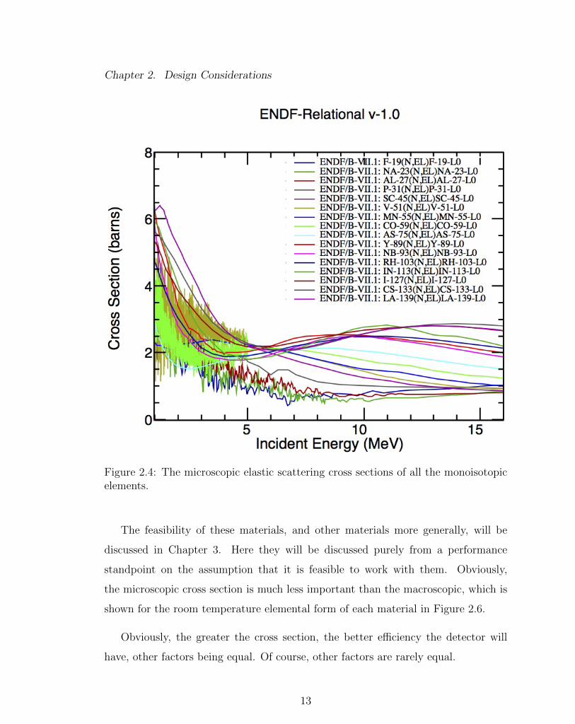
2.1.2 Cross Sections
This encompasses two variables of interest: the total cross section in the relevant
energy range, and the distribution of scattering angle. Neutron elastic scattering
cross sections range from 0.25 to 3 barns at 14.1 MeV, substantially impacting overall
e�ciency. For 2.45-MeV neutrons, the elastic scattering cross section tends to be
somewhat higher, with much more structure. Structure in the cross-sections is not
inherently a problem, but any error in resolving that structure will translate to
artificial structure in the measured spectrum, since the spectrum must be corrected
for the changing cross section over energy. Figure 2.4 below shows the microscopic
scattering cross sections for all the monoisotopic elements, from 1 MeV to 16 MeV.
While these di↵erences are nontrivial, in practice they are subsumed by the dif-
ficulty of working with some materials. For example, depositing a submicron-thick
layer of sodium on a surface, with no coating, is impractical from a chemical stand-
point, regardless of cross sections. Constructing a pure fluorine “foil” would be
impossible.
Foils with multiple isotopes could potentially function, but the di↵erence in cross-
section and distributions of scattering angles (the latter particularly significant at low
mass) would reduce performance. It is also possible to get isotopically pure samples
of non-monoisotopic elements, in which case a large number of isotopes could be
considered, far beyond the scope of this work. Fortunately, the monoisotopic elements
span a wide range of masses, and have reasonable elastic scattering cross-sections,
so a selection of monoisotopic elements is su�cient for demonstrating this detector
concept. For the remainder of the chapter, six elemental materials will be considered
as plausible examples, to give a sense of the range of performance that is achievable.
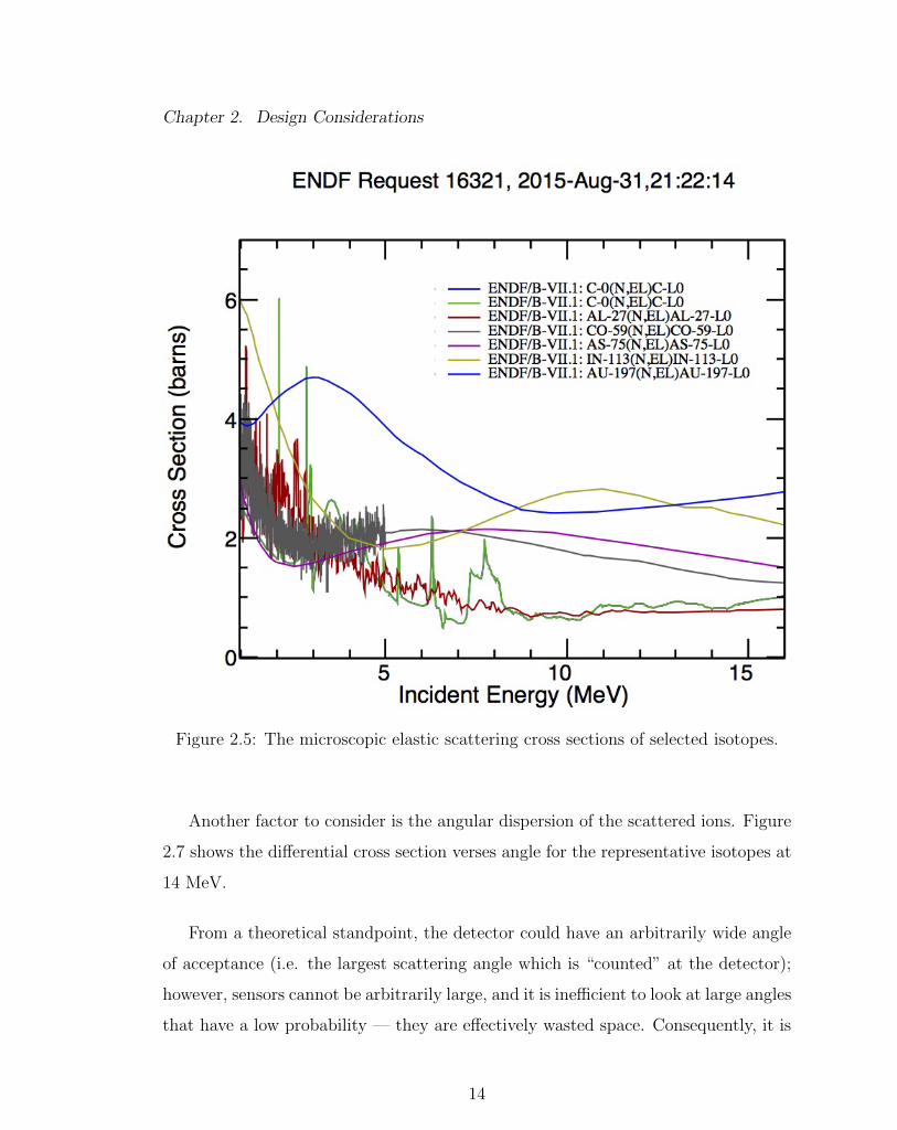
These materials are carbon, aluminum, cobalt, arsenic, indium, and gold. Figure 2.4
is repeated below with just these isotopes.
12
Chapter 2. Design Considerations
Figure 2.4: The microscopic elastic scattering cross sections of all the monoisotopicelements.
The feasibility of these materials, and other materials more generally, will be
discussed in Chapter 3. Here they will be discussed purely from a performance
standpoint on the assumption that it is feasible to work with them. Obviously,
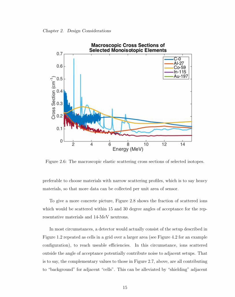
the microscopic cross section is much less important than the macroscopic, which is
shown for the room temperature elemental form of each material in Figure 2.6.
Obviously, the greater the cross section, the better e�ciency the detector will
have, other factors being equal. Of course, other factors are rarely equal.
13
Chapter 2. Design Considerations
Figure 2.5: The microscopic elastic scattering cross sections of selected isotopes.
Another factor to consider is the angular dispersion of the scattered ions. Figure
2.7 shows the di↵erential cross section verses angle for the representative isotopes at
14 MeV.
From a theoretical standpoint, the detector could have an arbitrarily wide angle
of acceptance (i.e. the largest scattering angle which is “counted” at the detector);
however, sensors cannot be arbitrarily large, and it is ine�cient to look at large angles
that have a low probability — they are e↵ectively wasted space. Consequently, it is
14
Chapter 2. Design Considerations
Figure 2.6: The macroscopic elastic scattering cross sections of selected isotopes.
preferable to choose materials with narrow scattering profiles, which is to say heavy
materials, so that more data can be collected per unit area of sensor.
To give a more concrete picture, Figure 2.8 shows the fraction of scattered ions
which would be scattered within 15 and 30 degree angles of acceptance for the rep-
resentative materials and 14-MeV neutrons.
In most circumstances, a detector would actually consist of the setup described in
Figure 1.2 repeated as cells in a grid over a larger area (see Figure 4.2 for an example
configuration), to reach useable e�ciencies. In this circumstance, ions scattered
outside the angle of acceptance potentially contribute noise to adjacent setups. That
is to say, the complementary values to those in Figure 2.7, above, are all contributing
to “background” for adjacent “cells”. This can be alleviated by “shielding” adjacent
15
Chapter 2. Design Considerations
Figure 2.7: The di↵erential elastic scattering cross sections of selected isotopes.
cells from one another.
Combining the e↵ects from the previous two sections, a heavy foil material like
gold or indium seems like an obvious choice. Unfortunately, their benefits are coun-
terweighted by the problematic phenomenon of straggling, discussed in the next
section.
16
Chapter 2. Design Considerations
Figure 2.8: The accepted fraction for select materials with 15 and 30 degree anglesof acceptance.
2.1.3 Foil Thickness and Straggling
As the stream of scattered ions pass through the foil, several things happen. Most
obvious is the steady loss of energy through collisions with electrons in the foil —
as the foil thickness increases, the average energy of escaping ions rapidly declines.
More subtly, there is a small probability of the ion colliding with a nucleus in the
foil, resulting in a larger change in energy and an accompanying change in direction.
The thicker the foil, the more of these collisions occur, resulting in a process called
straggling. As a result, as the thickness of the foil increases, the width of the energy
distribution about the mean will increase, and more ions will be scattered o↵ their
initial course. This phenomena has large implications for the design of the heavy ion
17
Chapter 2. Design Considerations
recoil neutron spectrometer.
First, consider the steady energy loss. Since lower energy — and consequently
slower — ions are to the detector’s benefit, the intuitive conclusion is to find the
thickest foil from which nearly all ions could escape. Even ignoring potential strag-
gling e↵ects, this approach is foiled by the neutrons, which are equally likely to
scatter at any depth in the foil. As a result, for a thick foil, some neutrons will
scatter at the front of the foil, producing ions that lose nearly all their energy before
escaping, while other neutrons will scatter at the back of the foil, producing ions who
escape with all their energy intact.
On the other hand, the thicker the foil, the more neutrons interact, and the higher
the e�ciency of the detector. Consequently, the appropriate foil thickness depends
on the relative importance of e�ciency and energy resolution for a given situation.
Further complicating matters is the relationship between ion/material charge and
energy loss. The semiclassical formula for stopping power [11] gives a sense of how
energy loss will change with higher-z materials:
�dE
dx
=4⇡k2
0z2e
4n
mV
2ln(
mV
2
hf
) (2.2)
Where �dE
dx
is the stopping power, k0 is coulomb’s constant, z is the charge of the
ion, e is the electron charge, n is the electron density in the material (in this case,
equal to z), mV
2 is the ion’s kinetic energy, and f is the orbital frequency. At
a given ion energy, it suggests the stopping power increases with the cube of the
atomic number of the foil material. That is to say that, number densities being
equal, lower Z materials can be made thicker — leading to better e�ciency — than
high Z materials and retain comparable energy loss.
This leaves the phenomena of straggling. Energy straggling, fortunately, is ir-
relevant: the energy di↵erence between ions created at the front and back of the
18
Chapter 2. Design Considerations
foil exceed the straggling losses in the foil, so the straggling losses add no measur-
able e↵ect. Angular straggling is another matter. An ion scattering even a few
degrees from its original direction will introduce a substantial error, resulting in an
incorrectly calculated neutron energy.
It is useful to consider some specific examples to give a better sense of the impact.
Suppose a beam of 14-MeV neutrons is striking a foil with atomic mass M. If we
consider ions which are scattered straight forward, they will have an initial angle
of zero degrees and an energy dictated by Equation 1.5. Without straggling, on a
detector with infinite spatial and time resolution, every ion would be detected as
coming from a 14-MeV neutron.
First, consider the impact of energy loss. Since the neutron is equally likely
to scatter anywhere in the foil, the escaping ions will have a uniform energy dis-
tribution between their initial scattered energy E0 = 4mneutron
M
ion
(mneutron
+M
ion
)214MeV and
E = E0 � E
loss
, where E
loss
is the average energy loss of an ion passing through
the full thickness of the foil. This range can be characterized as a percentage of the
initial energy. Combining this with Equation 1.8 gives Figure 2.9, which shows the
measured spectrum of the uniform 14 MeV beam at foil thicknesses chosen to give a
minimum ion energy of 90%, 95%, 98%, and 99% of the initial energy.
Note that Figure 2.9 assumes all ions are scattered straight forward. When the
actual angular distribution is considered, the impact is greater: if the neutron-ion
collision scatters the ion to an angle of 30 degrees, the ion will have more material
to traverse, leading to greater energy loss and angular straggling.
Continuing on to angular straggling, which will be defined as the polar angle
between the ion’s trajectory when it is initially scattered and its trajectory when it
escapes the foil. Extending the scenario described above, where only ions scattered
at 0 degrees were considered, Figure 2.10 shows the measured energy spectrum of a
19
Chapter 2. Design Considerations
Figure 2.9: Measured spectra with various foil thicknesses, accounting for the distri-bution of energies of ions escaping the foil. For each case, the thickness was chosen sothat an ion scattered directly forward at the front of the detector would, on average,escape the foil with the labeled percentage of its initial energy.
foil thickness chosen to give an average straggling of 1�, 2�, 5�, an 10�, still assuming
the initial ions are all scattered directly forward (i.e. an initial angle of 0�).
Consider Equation 1.8 and Equation 1.6. The angle of scattering is coupled to the
energy of the ion by the laws of mechanics, so increasing the angle implies decreasing
the energy and consequently increasing t
arrival
. Angular straggling is equivalent to
changing ✓ in Equation 1.8 without changing t
arrival
. In the situation considered
above, the initial angle is zero degrees, so any change must be an increase in angle.
Without the accompanying change in the time of arrival, the calculated energy will
be higher than the actual energy.
20
Chapter 2. Design Considerations
Figure 2.10: Measured spectra with angular straggling with all ions initially scatteredinto a 0� angle.
Angular straggling has a much greater impact on measured energy if (for example)
it is a change from 20 degrees to 30 degrees than if it is a change from 0 degrees
to 10 degrees. Figure 2.11 shows the spectra resulting from the straggling described
above, but with an initial scattering angle of 20�. For consistency with the previous
scenario, the change in angle is always an increase, rather than being distributed
between increase and decrease as would physically happen.
The simplest way to put all of this together is with a simulation. Specifically,
Geant4 was used to simulate scattering of 14-MeV neutrons in cobalt 59. The foil
thickness of 6.106 nm was selected for an average outcoming energy of 98% of the
21
Chapter 2. Design Considerations
Figure 2.11: Measured spectra with angular straggling, with all ions initially scat-tered into a 20� angle.
initial scattered energy. Perfect spatial and time sensitivity was assumed, with an
acceptance angle of 30 degrees. For a more detailed discussion of the methodology,
see Chapter 4 as well as Appendix A. The detected spectrum, for 1.0x10⁷ scatters,
is shown in Figure 2.12.
The full-width-at-half-max (FWHM) measured is 0.476 MeV, with a mean of
13.953 MeV. This suggests that the 98% energy point is fairly reasonable thickness
to use. The down-shift in the average energy is due to the energy losses in the foil
— on average, the ions are created in the center of the foil and experiences some
energy loss before escaping the foil, translating to a low measured average energy.
22
Chapter 2. Design Considerations
Figure 2.12: Measured spectra with 6.106 nm Co foil.
With these results in mind, Table 2.1.3 shows the 95%, 98% and 99% energy foil
thicknesses for the isotopes under study, along with relevant peripheral information
about the materials.
23
Chapter 2. Design Considerations
Table 2.1: Shows the thickness for which the average outcoming energy is 99%, 98%,and 95% of the initial energy for several materials. All thicknesses are in nanometers.Source: SRIM [12]
The previous section discussed the implications of foil thickness to detector perfor-
mance. This section considers two further spatial design parameters: the area of the
foil, and the distance from the foil to the detector.
The implicit assumption in Equation 1.8 is that the ions scattered by the neutrons
are a point source. All of the calculations of distance, angle, and ultimately energy,
assume that the ion was scattered at the exact center of the foil. In reality, of course,
the ions are scattered randomly in the finite area of the foil. In fact, since the
e�ciency of the detector scales linearly with the area of the foil, it is preferable that
it be a relatively large area. As with every other aspect of the detector’s design, foil
area is a tradeo↵ between e�ciency and energy resolution.
This tradeo↵ is mitigated by distance. The loss in energy resolution correlates
not to the absolute area of the foil, but to the solid angle subtended by the foil at
the closest point on the sensor. That is to say, a 1 mm2 foil 2 cm from the sensor is
equivalent to a 2.5 mm2 foil 5 cm from the sensor, for purposes of uncertainty.
24
Chapter 2. Design Considerations
Increasing the distance also increases the e↵ective resolution. For a given absolute
sensor resolution, the further away the sensor is from the foil, the smaller the solid
angle of each detectable point, which means that each point/time combination aligns
with a narrower range of neutron energies, improving the measured energy resolution.
Finally, increasing the distance increases the time interval between when the neutrons
and gammas strike the sensor and when scattered ions strike the sensor.
As with all choices, moving the detector further away has substantial downsides.
Firstly, for a given angle of acceptance, the sensor area goes up with the square of
the distance. For most sensor technologies, large sensors are expensive and often
impractical. Secondly, greater spacing reduces the number of detector “units” that
can work in parallel, reducing overall e�ciency. (See Chapter 3 for further discussion
of this problem.)
For a concrete picture of the implications, consider a square foil 20 mm by 20 mm
(unreasonably large, but useful for demonstration) placed 10 cm from a sensor and
struck by 14-MeV neutrons. Once again, suppose cobalt is the foil material. Two
neutrons scatter o↵ the foil, producing ions: one scatters in the exact center of the
foil, the other scatters at its outer edge, but both ions are scattered toward the exact
center of the sensor. The situation is shown in Figure 2.13.
Both scattered neutrons had the same energy, 14 MeV, but scattered ions at
di↵erent angles. Equation 1.5 yields respective ion energies of 0.917778 and 0.917686
MeV. The ion from the center of the foil will arrive at the detector 57.718 ns after
scattering, while the ion from the edge will arrive 59.295 ns after scattering, 1.577
nanoseconds later. This is e↵ectively changing t
arrival
in Equation 1.8, resulting in
a change in the measured energy. Specifically, the ion that came from the center
of the foil will be correctly correlated to a 14-MeV neutron, while the second ion,
which came from the foil edge, will be calculated to have come from a 13.724 MeV
neutron. This error is exacerbated further from the center of the sensor: if both ions
25
Chapter 2. Design Considerations
Figure 2.13: Diagram showing scattering from di↵erent points on the foil to the samepoint on the sensor. Not to scale.
were scattered to a point 5.77 centimeters from the center of the sensor (a 30 degree
scatter coming from the center of the foil), the measured energies would have been
14 and 16.508 MeV.
Figure 2.14 gives a broader picture. It shows several spectra, from the configura-
tion discussed above but with several di↵erent foil sizes.
26
Chapter 2. Design Considerations
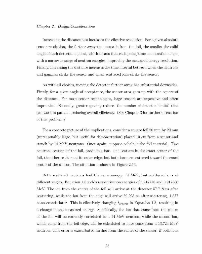
Figure 2.14: Measured spectra for various foil sizes, ignoring straggling losses.
Clearly, the detector resolution is less sensitive to this parameter than to most
others discussed in this chapter, but in high resolution contexts it becomes quite
significant. The measured FWHM ranges from 0.205 MeV with the 2 mm foil to
1.025 MeV for the 10 mm foil.
2.1.5 Noise
As discussed, the purpose of selecting a heavy material for the foil is so that the scat-
tered ions arrive at the sensor much later than the primary neutrons and bremsstrahlung,
to insure that they do not “white out” the useful signal. Unfortunately, the neu-
trons and bremsstrahlung produce secondary radiation lasting microseconds after
27
Chapter 2. Design Considerations
the primary burst.
There does not appear to be a detailed experimental time history examination of
the radiation environment at a suitable ICF facility — most sources cut o↵ after a few
tens of nanoseconds or less. In any case, it would be strongly geometry-dependent, so
comparison between such a source and the anticipated environment for this detector
would be questionable. This makes a detailed assessment of the impact on detector
performance di�cult, but some useful generalizations are helpful.
First, consider the time frame of interest for the detector. Table 2.2 shows the
peak time for a forward scattered ion to arrive at a sensor for the sample foil materials
at several foil to sensor distances, for both DD and DT sources, with a 5 cm foil to
sensor separation.
Table 2.2: Shows the most probable time of arrival (measured from when the scatteroccurs) for forward scattered ions (both DD and DT) to a sensor 5 cm away forseveral materials.Material Peak Energy
For heavier foil materials, or for configurations with large separation between the
foil and the sensor, it seems safe to presume most of the gamma signal will be gone.
For light foil materials, or short, distances, it could be a substantial concern, though
peripheral shielding could eliminate much of the problem.
This conclusion is largely supported by simulations done in support of an x-
ray streak camera designed for placement near Laser Megajoule facility in France
[3]. This facility is designed for ICF experiments similar to those undergone at the
National Ignition Facility, with implosions producing in excess of 1x10¹⁵ neutrons. In
30
Chapter 2. Design Considerations
assessing the dose to a CCD sensor roughly 3.4 meters from the implosion, the paper
suggests substantial gamma dose occurs for tens of nanoseconds after the primary
pulse, due to the di↵usion of the bremsstrahlung and secondary gammas. This is
consistent with the above estimations. Given that this detector would generally be
placed closer than 3 meters, it is probably a generous estimate.
In summary, while the noise from the high radiation environment is certainly
not negligible, and would merit substantial study before a detector was constructed,
there is no reason to believe it fatal to this detector design.
2.2 Sensor
2.2.1 Timing
Sensor timing limitations are probably the greatest bottleneck in the performance of
this type of spectrometer. Even if extremely heavy materials are selected for the foil,
the time between the slowest and fastest ions arrival at the detector is still only tens
of nanoseconds. This means that time bins have to be extremely narrow — preferably
sub-nanosecond — and having more time bins dramatically improves resolution of
the detector. On the other hand, the useful time resolution is inherently limited by
uncertainty: if the neutron source uncertainty is in the 10 nanosecond range, 100
picosecond timing resolution gives no useful benefit over 1 nanosecond resolution.
The chapter on feasibility will discuss what sort of timing is plausible with current
technology. For the present, it su�ces to analytically assess how timing characteris-
tics of the detector design impact overall performance.
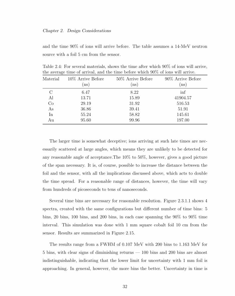
It is best to start by considering the timing variation for di↵erent materials. Table
2.4 shows the time 90% of ions will arrive after, the most probable time of arrival,
31
Chapter 2. Design Considerations
and the time 90% of ions will arrive before. The table assumes a 14-MeV neutron
source with a foil 5 cm from the sensor.
Table 2.4: For several materials, shows the time after which 90% of ions will arrive,the average time of arrival, and the time before which 90% of ions will arrive.
The larger time is somewhat deceptive; ions arriving at such late times are nec-
essarily scattered at large angles, which means they are unlikely to be detected for
any reasonable angle of acceptance.The 10% to 50%, however, gives a good picture
of the span necessary. It is, of course, possible to increase the distance between the
foil and the sensor, with all the implications discussed above, which acts to double
the time spread. For a reasonable range of distances, however, the time will vary
from hundreds of picoseconds to tens of nanoseconds.
Several time bins are necessary for reasonable resolution. Figure 2.3.1.1 shows 4
spectra, created with the same configurations but di↵erent number of time bins: 5
bins, 20 bins, 100 bins, and 200 bins, in each case spanning the 90% to 90% time
interval. This simulation was done with 1 mm square cobalt foil 10 cm from the
sensor. Results are summarized in Figure 2.15.
The results range from a FWHM of 0.107 MeV with 200 bins to 1.163 MeV for
5 bins, with clear signs of diminishing returns — 100 bins and 200 bins are almost
indistinguishable, indicating that the lower limit for uncertainty with 1 mm foil is
approaching. In general, however, the more bins the better. Uncertainty in time is
32
Chapter 2. Design Considerations
Figure 2.15: Measured spectra for di↵erent numbers of bins, neglecting straggling.
a significant complication. Uncertainty comes from any number of sources: duration
of the neutron source, jitter in timing equipment, and so on. Figure 2.16 shows
four spectra 20 (timing) bins wide. Each spectrum arises from a di↵erent (uniform)
timing uncertainty: 0 ps, 100 ps, and 500 ps, and 1000 ps.
Timing uncertainty decreases the accuracy, but not to an unreasonable degree.
Even with 2 nanoseconds of uncertainty, the resulting FWHM is only 0.683 MeV.
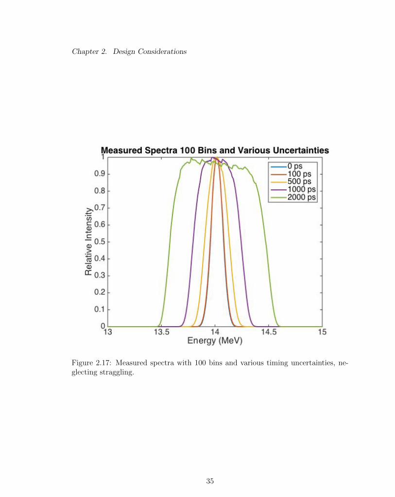
To get a sense of how number of bins impacts matters, Figure 2.17 shows four more
spectra, calculated using 100 bins, with the same uncertainties.
33
Chapter 2. Design Considerations
Figure 2.16: Measured spectra with 20 bins and various timing uncertainties, ne-glecting straggling.
34
Chapter 2. Design Considerations
Figure 2.17: Measured spectra with 100 bins and various timing uncertainties, ne-glecting straggling.
35
Chapter 2. Design Considerations
2.2.2 Pixel Size and Coverage
The next parameter to consider is the spatial resolution and coverage of the sensor.
If the sensor is a camera, the spatial resolution would be the pixel pitch, and the
coverage is simply the fraction of the sensor surface which is sensitive. Alternatively,
the sensor could be a diode array, in which case the spatial resolution is the spacing
between diodes, and the coverage is the area of the sensor which is sensitive diode
divided by the total area.
The significance of the coverage is intuitive: the e�ciency of the detector is
proportional to the coverage, since every ion scattered into a non-sensitive region is
lost. Furthermore, dead space between sensitive regions also decreases the spatial
resolution. Obviously, it is desirable to maximize coverage.
On the other hand, detector performance is insensitive to a wide range of spa-
tial resolutions. This is because of solid angle. Any reasonable design will have a
relatively large foil — typically at least 1 mm2. With a camera, spatial resolution
will almost always be in the um range, which means that spatial uncertainty due to
spatial resolution is overshadowed by uncertainty from foil size. Even if an infinitely
narrow foil were plausible, angular straggling contributes more spatial uncertainty
than the resolution: 1 degree of scatter, at 5cm, equates to 873 um di↵erence in
where the ion impacts the sensor. In the case that diodes are used (see the feasibil-
ity section for more on the distinction), larger pixels are probable, but will still be
similar to or smaller than the foil size.
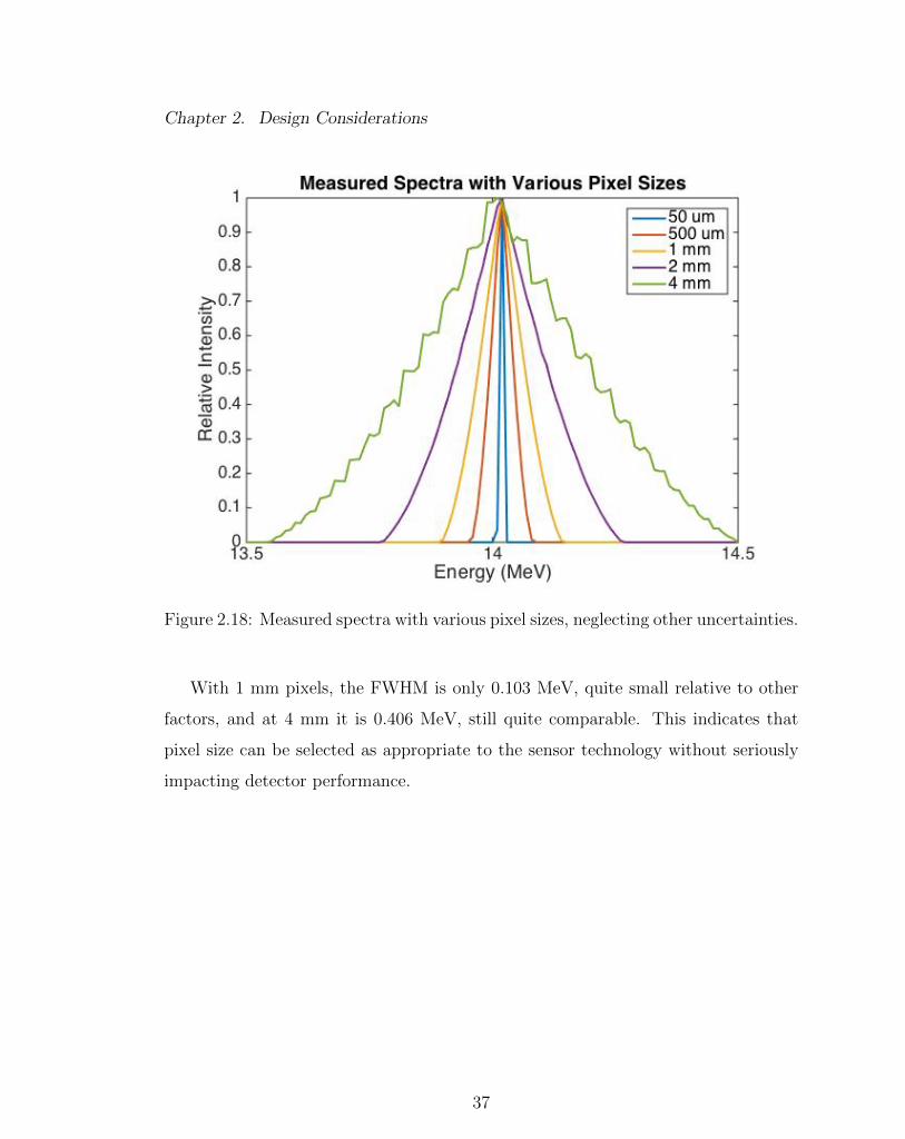
To isolate spatial resolution, consider a hypothetical configuration with a point-
foil, so that the foil contributes no spatial uncertainty, and an infinitely thin foil, so
there is no straggling — in short the scattered ions are coming from a point source.
The configuration will use cobalt foil, 10 cm from the sensor. Figure 2.18 shows the
resulting spectra, with several di↵erent spatial resolutions.
36
Chapter 2. Design Considerations
Figure 2.18: Measured spectra with various pixel sizes, neglecting other uncertainties.
With 1 mm pixels, the FWHM is only 0.103 MeV, quite small relative to other
factors, and at 4 mm it is 0.406 MeV, still quite comparable. This indicates that
pixel size can be selected as appropriate to the sensor technology without seriously
impacting detector performance.
37
Chapter 3
Feasibility
3.1 Fielding Environment
Any discussion of feasibility must start by considering useful cases. This detector
is only useful for very short pulses of neutrons — it would be useless at the Joint
European Torus. It will also have a very low e�ciency, so it needs to be fielded with
a large neutron source. With these considerations, two prime options for fielding are
the Z Machine, at Sandia National Laboratories, and the National Ignition Facility,
at Livermore National Laboratories.
The Z Machine has a record neutron yield of 4x10¹³, while the National Ignition
Facility has a record neutron yield of 9x10¹⁵, so a feasible detector must have a
high enough e�ciency to work somewhere in this range. In both cases, experiments
can potentially fielded roughly 30 cm from the implosion. Being closer improves
e�ciency, so the detector needs to be able to survive placement near the implo-
sion. Finally, neither facility produces delta sources of neutrons. The Z Machine
produces neutron bursts averaging tens of nanoseconds long, while the National Ig-
nition Facility implosions are generally less than one nanosecond. With this range of
38
Chapter 3. Feasibility
fielding environments as a baseline, this chapter discusses the feasibility of operating
a heavy-ion recoil neutron spectrometer.
3.2 Thin Foil Target
For a wide range of material/backing pairs, the requirements of this detector are well
within normal parameters. For this type of small-area thin-film, the most probable
technology to use would be ablation deposition. In this case, the surface to be coated
(the substrate) and a block of the coating material are placed in a vacuum chamber,
a short distance apart. The coating material is ablated, generally using a laser. The
resulting plasma expands, depositing a thin layer on the nearby substrate.
Because the process consists of ablating material which is then deposited, thin
coatings are generally discussed in terms of required mass per unit area, typically
micrograms per square centimeter. For the isotopes discussed in the previous sec-
tions, assuming a foil thickness between 1 and 10 nm thick, the equivalent coating
mass is in the range of 1 to 10 micrograms per square centimeter. This is well within
the normal achievable range, and does not present a problem [9].
In terms of material selection and viability, there are three primary factors to
consider: how amenable the coating material is to ablation, the amount of surface
area to be coated, and the permeability of the substrate. Most of the materials under
consideration are metals, and ablate well. Carbon is a nonmetal, but also works fine
for these types of thin coatings [9]. The detector requires a small surface area to
be covered, not more than one square centimeter for most plausible designs; this is
significant because the resulting small solid angle increases the achievable uniformity
of the coating. Finally, appropriate substrates can easily be chosen: lead is likely to
work, copper is a common choice, and many others are feasible.
39
Chapter 3. Feasibility
In short, the thin coatings requirements are a non-issue.
3.3 Sensor
3.3.1 Technology
The sensor has to be space and time resolved, and take multiple readings over the
span of a few nanoseconds. There are relatively few technologies that can hope
to meet this mix of criteria, but two are under development at Sandia National
Laboratories: a sub-nanosecond multi-frame camera, UXI [6], and a fast diode array
system based on the PSEC4 chip [8].
The camera has been developed for low energy x-ray sensitivity, but the technol-
ogy for ion sensitivity is fundamentally the same. Furthermore, since this camera was
developed with the expectation that it would be fielded in a neutron environment it
is expected to perform relatively well in the intense conditions the detector will need
to endure.
The fast diode array concept is not as well developed, but shows great promise.
The premise is that a large number of fast diodes are placed in a grid on a chip,
making the “sensor”. These diodes are then connected to an array of PSEC4 chips,
which act as “scopes on a chip”, allowing for a large number of reads in a short time.
3.3.2 Time Resolution
The current iteration of UXI can collect four frames. Each frame has a one nanosec-
ond integration time, and is separated from the next from by a minimum one nanosec-
ond recovery time. To get a reasonable number of time bins, multiple foil/sensor pairs
40
Chapter 3. Feasibility
would have to be fielded, but that is necessary for e�ciency anyway. The minimum
resolution (that is, the minimum integration time) is enough, barely, for some useful
data; however, for good resolution it would have to be improved. The goal of the
project is to reach sub-nanosecond timing. As the achievable integration time gets
shorter, the camera will quickly become a more appealing option.
The PSEC4-based diode array has much better timing characteristics: 256 bins
70 ps wide. This spans enough time ( 18 ns) to cover the whole pulse for reasonable
diode distance and foil material, and still gives time bins down at or below the width
of the time uncertainty. From this perspective, the diode array is obviously the
superior choice.
The problem comes from trying to synchronize a large number of diodes on a
large number of PSEC4 chips. UXI, as a camera, is designed from the ground up so
that all pixels have the same timing alignment; in spite of this it has an end-to-end
timing uncertainty in the vicinity of 100 ps. Getting that kind of timing alignment
out of a large number of PSEC4 chips, all at the same once, will be a di�cult task.
3.3.3 Spatial Resolution and Coverage
From a spatial resolution perspective, the UXI camera is perfect, if not overkill. With
35 um pixels, it is well below the uncertainty level from the foil and the angular
straggling. The full coverage is excellent, and means no ions are lost “in the cracks”.
A board could be designed with multiple UXI sensors edge-to-edge, for a larger
e↵ective sensor.
The diode array is trickier. Depending on the details of the design, the diodes can
reasonably have a fill factor in the vicinity of 80%, which is not perfect, but is a fairly
small contribution to e�ciency relative to other factors. The main challenge comes
from the sheer number of diodes required, combined with the small diodes necessary
41
Chapter 3. Feasibility
for good performance. The time response of a diode is proportional to the diode’s
area. At 2 mm, which is a fairly large diode, the sensor will have 25 diodes per
square centimeter. Since the smallest conceivable geometry will have several square
centimeters of sensor, and a plausibly e�cient design will repeat this arrangement
dozens of times, the result is thousands of diodes, with a PSEC4 chip, or something
comparable, for every few diodes. While there is no hard limit on how many diodes
is feasible, at some point it becomes infeasible from a design standpoint. At that
point, the practical solution is to reduce the fill factor, spacing out the diodes over
the area rather than packing it. In this case, e↵ective fill factor might be reduced
dramatically, with a corresponding reduction in e�ciency.
3.3.4 Radiation Hardness and Survivability
This is the most di�cult area to assess, for the simple reason that very little testing
has been done to assess the performance of either the UXI camera or most diodes
in a high-gamma, high-neutron environment. Until there is empirical data, the best
that can be done is consider these types of devices in general.
While there is limited data on fielding silicon detectors at the National Ignition
Facility or the Z Machine, considerable simulation work has been done in preparation
for fielding a high-speed CMOS streak camera for x-ray diagnostics on the Laser
Megajoule facility in France [3]. This facility is similar to the National Ignition
Facility, designed for ICF experiments producing in excess of 1x10¹⁵ neutrons. Rather
than attempting to design a CMOS detector capable of withstanding these extreme
conditions, this team focused on simulated shielding requirements. While their sensor
was placed relatively far from the implosion (3.4 meters), their shielding requirements
give a sense of what would be needed here. To shield the x-rays and gammas down
to acceptable levels, they required 11.5 mm of lead in front of their detector, and
42
Chapter 3. Feasibility
3.5 mm of lead surrounding the rest of the detector. Thicker layers would be needed
for the present case; however, as the particle of interest is neutrons, not x-rays, a
much thicker layer of lead can be used before the neutron signal is unacceptably
attenuated.
Alternatively, the detector itself can be designed with radiation hardness in mind.
The large hadron collider uses a large number of silicon detectors, which must survive
even harsher environments than those of NIF. The design goals there are silicon
detectors that can survive fluxes of 1016 n1MeV equivalent
/cm2 over long periods of
time. A foil at 30 cm from a record-setting implosion on NIF would receive little
more than 1012 n/cm2, suggesting that silicon diodes that can survive pulsed power
experiments are definitely achievable. Li discusses several techniques which have
allowed diodes to reach the desired hardness to neutron radiation [7]. While data on
the gamma pulse from NIF is less clear, the same research teams for the LHC have
developed oxygenated silicon didoes that are nearly immune to radiation damage
from gamma rays [7].
The controlling electronics are also potentially sensitive to radiation damage,
and are likely to need replaced periodically; however, most problems from radiation
exposure are transient e↵ects immediately upon radiation. Since the useful signal
arrives substantially after the primary pulse, these transient e↵ects are not expected
to cause major problems on individual experiments.
Overall, while it is unclear whether hardware available right now would be e↵ec-
tive in the extreme conditions necessary for the spectrometer, and it is likely that
some components of the detector would need to be replaced frequently, the sensor
technology to survive fielding on ICF experiments is within reach.
43
Chapter 4
Anticipated Performance
4.1 Introduction
This chapter puts together all of the details and considerations of the previous
sections into two feasible designs and discusses their simulated performance. The
presented designs are not proposed detectors to be constructed; rather, they are
“sketches” of designs, meant to di↵use the many variables, possibilities, and limita-
tions discussed into two designs, aimed at high e�ciency and high resolution. This
enables discussion of overall performance for feasible designs.
In choosing parameters for the designs to discuss, there are many areas, as dis-
cussed in the previous chapter, where the current limits on what is possible are not
known — there simply is not enough data available. In general, the chosen con-
straints are based on what is reasonably considered achievable with moderate e↵ort,
rather than what could be fielded tomorrow. This is in keeping with the purposes of
this paper, which is to illustrate the potential of a novel design.
As a reference for feasible size and placement, both designs are intended roughly
44
Chapter 4. Anticipated Performance
as “drop-in” replacements for the magnetic recoil spectrometer at the national ig-
nition facility, which is described in detail in [4]. Based on this requirement, both
designs will fit in roughly a 30 cm by 30 cm by 100 cm volume, roughly 30 cm from
the implosion. In keeping with the configurations presented in [4], the two setups dis-
cussed are aimed, respectively, at maximizing resolution, while maintaining a feasible
e�ciency, and maximizing e�ciency, while maintaining a useful resolution.
4.2 Methodology
The performance of the configurations was simulated using Geant4 and Matlab.
Geant4 is a set of open source libraries for Monte Carlo simulation, implemented
in C++ [1]. Matlab is a commercial numerical integrated development environment
and computing language, used under an academic license.
Geant4 supports arbitrarily complex geometries, with source particles ranging
from neutrons and protons to optical photons to exotic high-energy hadrons. While
it originated at CERN for use in High Energy Physics research, it has been adopted
and expanded by research groups in a wide range of fields, ranging from medical
physics to semiconductor design. Di↵erent groups have extended the physics models
as appropriate to their various fields. For this project, most of the physics were
provided by the Livermore Low Energy Electromagnetic Models for charged particles,
which are well tested and validated [2].
While Geant4 also provides high-precision neutron libraries based on the ENDF-
B/VII data, the low elastic scattering cross section made doing a large number of
tests and simulations impractical. Instead, ions of the appropriate type were pro-
duced directly as primary particles. For each foil material, the angular scattering
distribution at 14 MeV and 2.45 MeV was inputted into the code — over the narrow
energy variations relevant to these experiments, the angular distribution is insensi-
45
Chapter 4. Anticipated Performance
tive. In a real detector, the slight structure in angular distribution as a function of
energy would be corrected in the same way as energy variations in cross sections.
By producing ions directly, both of these corrections are skipped. In a real system,
both would contribute to the overall uncertainty of the detector; however, this thesis
does not attempt to assess the uncertainty of performance, since to many variables
are unknown and impossible to meaningfully estimate. Consequently, producing the
ions directly does not impact the simulated performance of the detector.
For a given configuration, the ions are randomly generated within the space of the
foil. The polar angle is sampled from the angular distribution, while the azimuthal
angle is randomly sampled between 0 and 2⇡. The energy corresponding to the
sampled polar angle is calculated, and the particle is sent into the simulation. There
is also a provision to set the start time of the particle, to simulate a neutron source of
finite duration. This setup allows for force conditions to be implemented, to isolate
the source of di↵erent behaviors: it can easily be changed to a point source, rather
than a spatial source, to see what di↵erence the foil makes, or the foil can be replaced
with vacuum, to test the impact of straggling, and so on.
The detector is a rectangular prism, parallel to the foil, at a distance determined
by the configuration. Geant4 is configured to tally at what point each ion enters the
detector, and at what time. This information is recorded for every simulated ion and
written to a file at the end of the simulation.
This data is then read into Matlab, where it is binned based on the defined
specifications of the configuration. Detector response, or non-ideal factors, could
also be implemented at this stage; however, for purposes of these tests, it is assumed
that the detector responds ideally, or could be corrected to ideal response. In this
way, several detector resolutions, in both time and space, could be tested without
re-simulating the physics.
46
Chapter 4. Anticipated Performance
Appendix A contains a partial code listing for more implementation detail.
4.3 High Resolution Configuration
4.3.1 Setup
Based on earlier chapters, optimizing resolution requires minimizing foil and pixel
size while using a large number of time bins with short duration relative to the
spread of time-of-arrival for the ions. Furthermore, thin foil is preferable to minimize
ion straggling. Balancing these requirements and the need for a feasible e�ciency,
the chosen configuration uses a 2 mm by 2mm by 2 nm cobalt foil, 10 cm from
a diode array sensor. With a narrow, 15� angle of acceptance, the sensor consists
of 729 diodes, each 2 mm by 2mm in size, forming a grid 5.4 cm on a side. This
is more than could reasonably be accommodated by existing digitizing chips, but
could plausibly be accommodated with an expanded version of the technology in
PSEC4 chips. Based on existing hardware, it will be assumed that each diode has a
limit of 70 ps samples, with 256 samples. While traditional diodes of this size could
not achieve these speeds due to capacitance, it is achievable with three-dimensional
diodes similar to those developed at CERN. The arrangement is shown in Figure4.1.
This configuration will form as a single “cell”. Over the available volume, it is
repeated in a grid to achieve usable e�ciencies. It will be assumed that each “cell”
is isolated from its neighbors (e.g. by thin partial walls extending from the borders),
so that there is no appreciable crosstalk between cells. Each cell is geometrically
identical, but the timing configuration for each is adjusted based on its location
relative to the source. In reality, each cell would also be angled slightly relative to
the source to maintain perpendicularity to the source; but this is not reflected in
Figure 4.2, showing the configuration.
47
Chapter 4. Anticipated Performance
Figure 4.1: A single cell of the high resolution configuration.
Figure 4.2: Full view of the high resolution configuration.
48
Chapter 4. Anticipated Performance
A flat-field gaussian fusion source provides the neutrons. Tests were done with
both DD and DT sources, at 5 keV and 10 keV. Each of these was then done with 0
ps, 500 ps, 1000 ps, and 2000 ps of uniform uncertainty in source time. While most
real sources are probably closer to gaussian in time, this is intended to also roughly
account for timing uncertainty in circuitry and other sources. This results in a total
of 12 tests for this configuration, and a thorough picture of performance.
4.3.2 Performance
While there are lots of graphs and pictures to consider, it is desirable to begin with a
concrete description of performance relative to a known standard. This is provided
by direct comparison to the existing spectrometer at the National Ignition Facility,
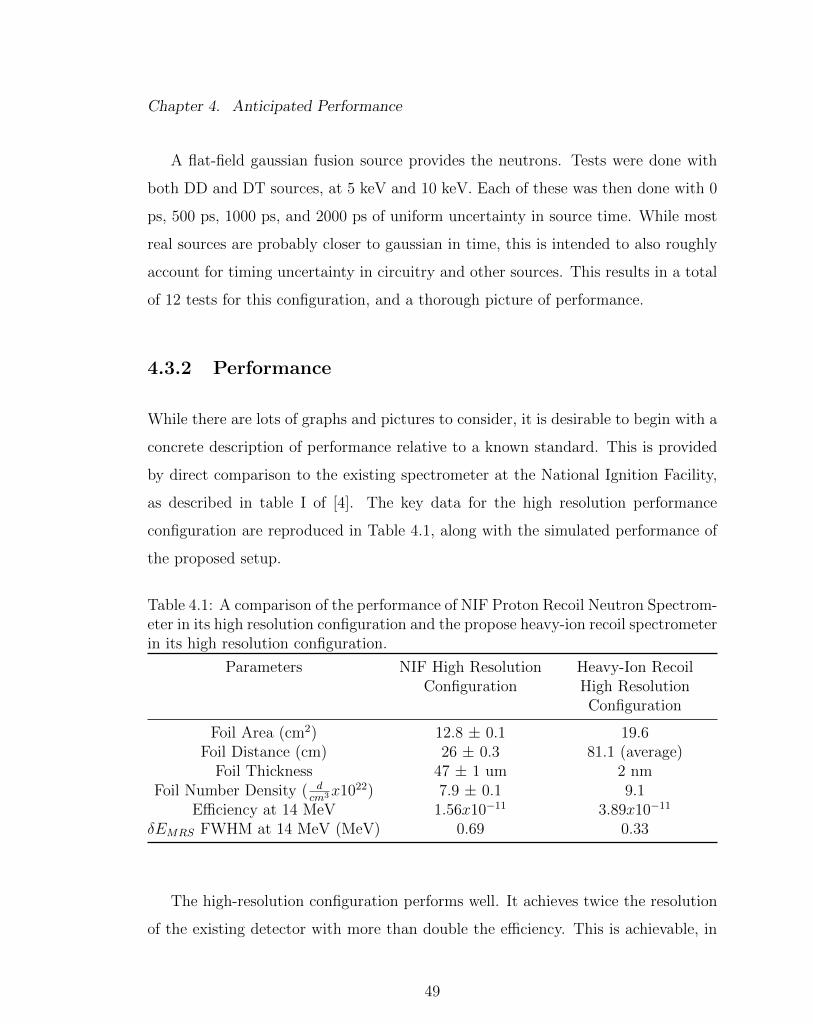
as described in table I of [4]. The key data for the high resolution performance
configuration are reproduced in Table 4.1, along with the simulated performance of
the proposed setup.
Table 4.1: A comparison of the performance of NIF Proton Recoil Neutron Spectrom-eter in its high resolution configuration and the propose heavy-ion recoil spectrometerin its high resolution configuration.
3x10²²) 7.9 ± 0.1 9.1E�ciency at 14 MeV 1.56x10�11 3.89x10�11
�E
MRS
FWHM at 14 MeV (MeV) 0.69 0.33
The high-resolution configuration performs well. It achieves twice the resolution
of the existing detector with more than double the e�ciency. This is achievable, in
49
Chapter 4. Anticipated Performance
spite of foil 4 orders of magnitude thinner than the existing NIF detector, because of
the much wider acceptance angle. While this is a comparison of a fully designed and
functional detector to a sketch of a detector concept, it indicates that the heavy-ion
Recoil spectrometer could operate in the same league as existing designs, and likely
at least incrementally better.
While clear and pleasantly quantifiable, this assessment says little about perfor-
mance in measuring a real spectrum, arriving over a much wider time interval than
a perfect, 14 MeV beam. Since timing is key for this detector, it is appropriate
to consider more realistic assessments. For example, a key performance question is
how much timing uncertainty the detector can accommodate and still provide useful
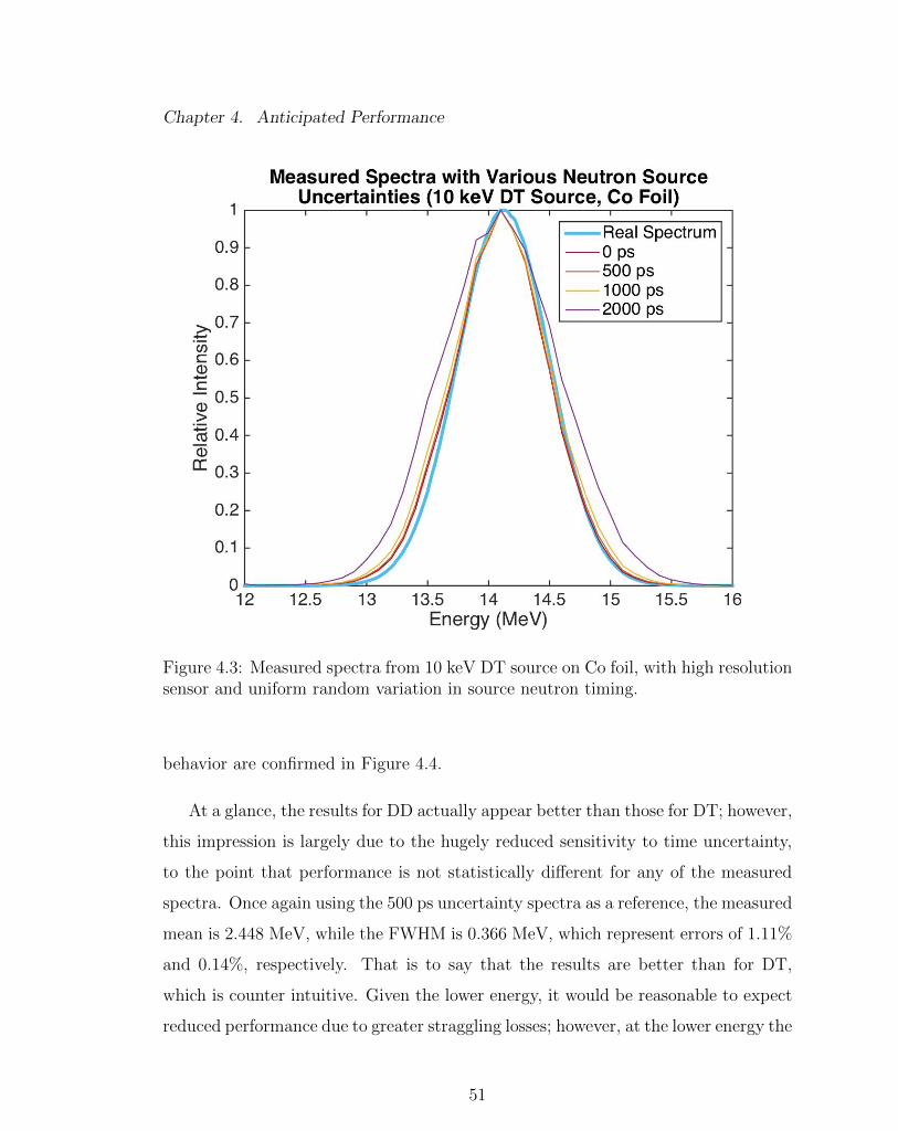
results. Figure 4.3 shows several spectra: the actual, generated DT spectra, along
with the spectra as measured with the various timing spreads discussed above.
Visual inspection is encouraging. It appears to be a good fit, and can weather
considerable timing uncertainty before performance is dramatically impacted. More
concretely, with 500 ps uncertainty the measured mean is 14.087 MeV with a full
width at half max (FWHM) of 0.847 MeV, an error of 7.98% in the FWHM and
0.20% in the mean. Most of the error in the FWHM is due to the systematically
down-shifted spectrum at lower energies. The systematically low mean is due to the
straggling energy loss in the foil, which causes the calculated neutron energy to be
slightly low; this e↵ect will be more pronounced at the lower energies of DD ions.
Overall, performance is consonant with what would be expected from the 14 MeV
performance in table 4.1.
Since DD neutrons are of much lower energy, there is a wider time spread for
DD neutrons on a given detector geometry, so for DD measurements on the cobalt
foil, the duration of the time bins was increased to 120 ps to fully span the range of
arrival times. Measurements of slow DD ions are less impacted by time uncertainty,
so dramatically better performance with large time spreads is to be expected. This
50
Chapter 4. Anticipated Performance
Figure 4.3: Measured spectra from 10 keV DT source on Co foil, with high resolutionsensor and uniform random variation in source neutron timing.
behavior are confirmed in Figure 4.4.
At a glance, the results for DD actually appear better than those for DT; however,
this impression is largely due to the hugely reduced sensitivity to time uncertainty,
to the point that performance is not statistically di↵erent for any of the measured
spectra. Once again using the 500 ps uncertainty spectra as a reference, the measured
mean is 2.448 MeV, while the FWHM is 0.366 MeV, which represent errors of 1.11%
and 0.14%, respectively. That is to say that the results are better than for DT,
which is counter intuitive. Given the lower energy, it would be reasonable to expect
reduced performance due to greater straggling losses; however, at the lower energy the
51
Chapter 4. Anticipated Performance
Figure 4.4: Measured spectra from 10 keV DD source on Co foil, with diode sensorand uniform variation in source neutron timing.
straggling losses are more uniform across the relevant energy spectrum. As a result,
rather than a downshifted low end, the DD data are almost uniformly downshifted,
leading to a more accurate FWHM measurement.
Finally, the pragmatic question from a fusion energy perspective: can this detec-
tor distinguish spectra for di↵erent fusion temperatures. The answer, fortunately,
is yes, even with fairly substantial uncertainties, but identifying the temperatures is
somewhat harder than di↵erentiating them. Figures 4.5 and 4.6 show measured 5
and 10 keV spectra with 500 ps timing uncertainties for DT and DD neutrons and
cobalt foil.
52
Chapter 4. Anticipated Performance
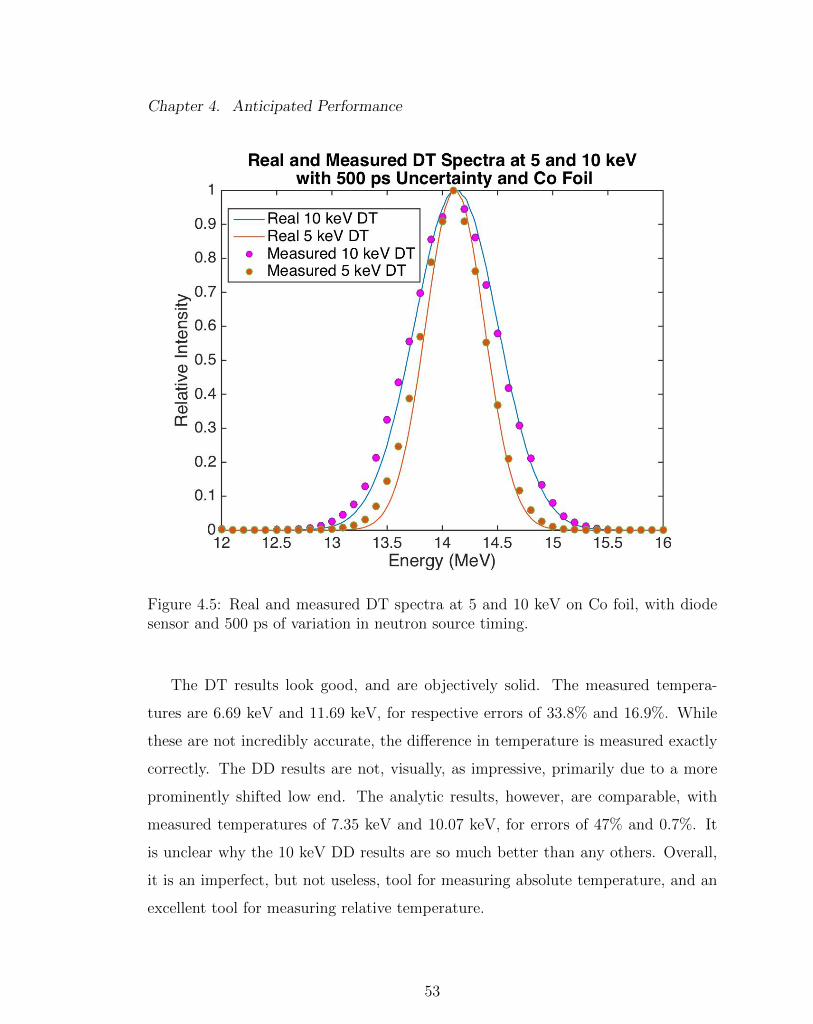
Figure 4.5: Real and measured DT spectra at 5 and 10 keV on Co foil, with diodesensor and 500 ps of variation in neutron source timing.
The DT results look good, and are objectively solid. The measured tempera-
tures are 6.69 keV and 11.69 keV, for respective errors of 33.8% and 16.9%. While
these are not incredibly accurate, the di↵erence in temperature is measured exactly
correctly. The DD results are not, visually, as impressive, primarily due to a more
prominently shifted low end. The analytic results, however, are comparable, with
measured temperatures of 7.35 keV and 10.07 keV, for errors of 47% and 0.7%. It
is unclear why the 10 keV DD results are so much better than any others. Overall,
it is an imperfect, but not useless, tool for measuring absolute temperature, and an
excellent tool for measuring relative temperature.
53
Chapter 4. Anticipated Performance
Figure 4.6: Real and measured DD spectra at 5 and 10 keV on Co, with diode sensorand 500 ps of variation in neutron source timing.
4.4 High E�ciency Configuration
4.4.1 Design
This configuration faces the inverse problem of the high resolution configuration:
getting the e�ciency as high as possible while keeping moderately useful resolution.
While nearly every design parameter impacts e�ciency to some degree, the single
greatest factor is foil dimensions. E�ciency increases as the cube of the foil volume,
so increasing a high e�ciency design is primarily about making the foil as large and
54
Chapter 4. Anticipated Performance
thick as possible without compromising too much performance. With this in mind,
a lighter foil material is obviously desirable. The resulting design uses a 10 mm by
10 mm by 25 nm carbon “foil” 10 cm from a diode detector. The diode detector
will be configured exactly the same as in the high e�ciency detector — meaning
that the two foils could be easily switched out to go from “high e�ciency” to “high
resolution” modes. Likewise, the same sources are used as above. The resulting cell
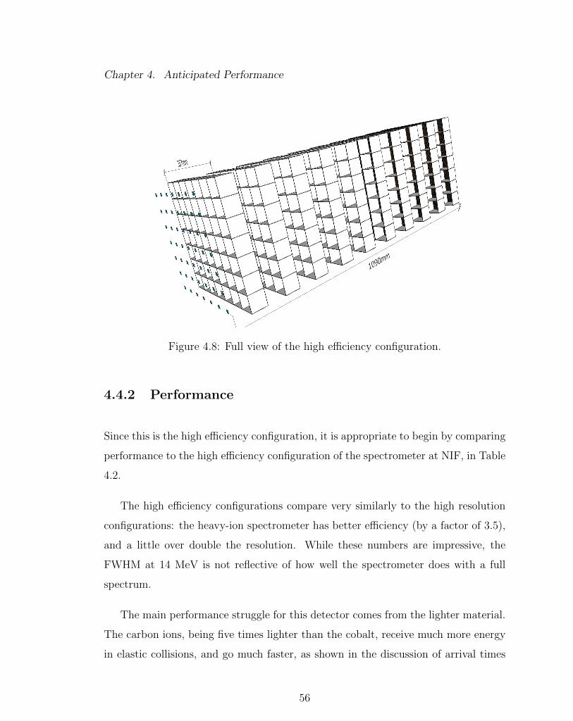
geometry and complete arrangement are shown in Figures 4.7 and 4.8.
Figure 4.7: A single cell of the high e�ciency configuration.
55
Chapter 4. Anticipated Performance
Figure 4.8: Full view of the high e�ciency configuration.
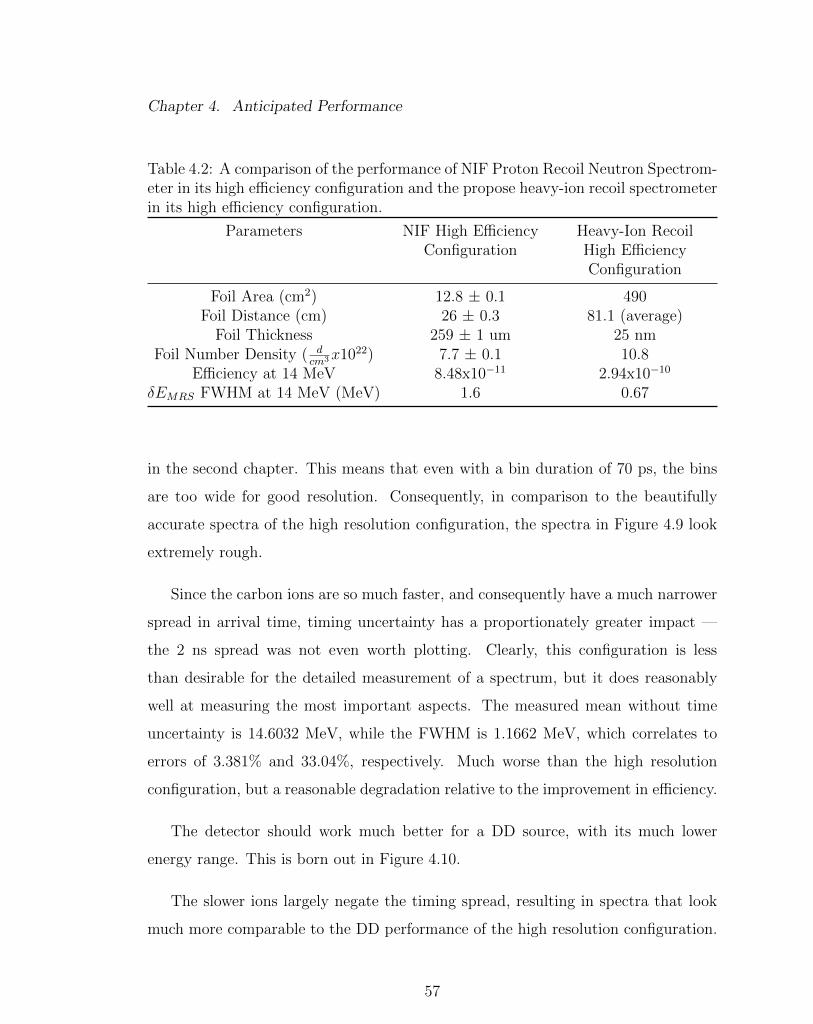
4.4.2 Performance
Since this is the high e�ciency configuration, it is appropriate to begin by comparing
performance to the high e�ciency configuration of the spectrometer at NIF, in Table
4.2.
The high e�ciency configurations compare very similarly to the high resolution
configurations: the heavy-ion spectrometer has better e�ciency (by a factor of 3.5),
and a little over double the resolution. While these numbers are impressive, the
FWHM at 14 MeV is not reflective of how well the spectrometer does with a full
spectrum.
The main performance struggle for this detector comes from the lighter material.
The carbon ions, being five times lighter than the cobalt, receive much more energy
in elastic collisions, and go much faster, as shown in the discussion of arrival times
56
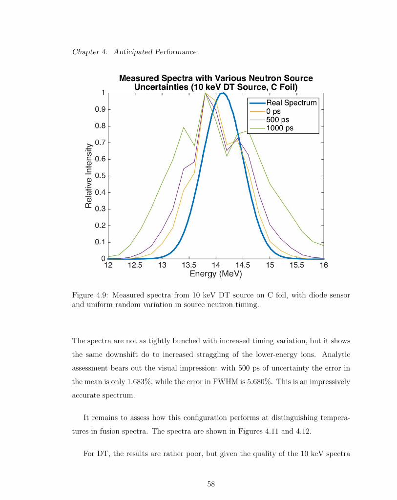
Chapter 4. Anticipated Performance
Table 4.2: A comparison of the performance of NIF Proton Recoil Neutron Spectrom-eter in its high e�ciency configuration and the propose heavy-ion recoil spectrometerin its high e�ciency configuration.