A Numerical Algorithm for Modeling Multigroup Neutrino-Radiation Hydrodynamics in Two Spatial Dimensions F. Douglas Swesty and Eric S. Myra Department of Physics and Astronomy, State University of New York at Stony Brook, Stony Brook, NY 11794–3800 [email protected][email protected]ABSTRACT It is now generally agreed that multidimensional, multigroup, radiation hydrodynamics is an indispensable element of any realistic model of stellar-core collapse, core-collapse super- novae, and proto-neutron star instabilities. We have developed a new, two-dimensional, multi- group algorithm that can model neutrino-radiation-hydrodynamic flows in core-collapse su- pernovae. Our algorithm uses an approach that is similar to the ZEUS family of algorithms, originally developed by Stone and Norman. However, we extend that previous work in three significant ways: First, we incorporate multispecies, multigroup, radiation hydrodynamics in a flux-limited-diffusion approximation. Our approach is capable of modeling pair-coupled neutrino-radiation hydrodynamics, and includes effects of Pauli blocking in the collision in- tegrals. Blocking gives rise to nonlinearities in the discretized radiation-transport equations, which we evolve implicitly in time. We employ parallelized Newton-Krylov methods to obtain a solution of these nonlinear, implicit equations. Our second major extension to the ZEUS algo- rithm is inclusion of an electron conservation equation, which describes evolution of electron- number density in the hydrodynamic flow. This permits following the effects of deleptoniza- tion in a stellar core. In our third extension, we have modified the hydrodynamics algorithm to accommodate realistic, complex equations of state, including those having non-convex be- havior. In this paper, we present a description of our complete algorithm, giving detail suffi- cient to allow others to implement, reproduce, and extend our work. Finite-differencing details are presented in appendices. We also discuss implementation of this algorithm on state-of- the-art, parallel-computing architectures. Finally, we present results of verification tests that demonstrate the numerical accuracy of this algorithm on diverse hydrodynamic, gravitational, radiation-transport, and radiation-hydrodynamic sample problems. We believe our methods to be of general use in a variety of model settings where radiation transport or radiation hydrody- namics is important. Extension of this work to three spatial dimensions is straightforward. Subject headings: hydrodynamics — radiative transfer — methods: numerical — supernovae: general — stars: collapsed — stars: interior Submitted to The Astrophysical Journal
Transcript
A Numerical Algorithm for Modeling Multigroup Neutrino-Radiation Hydrodynamics inTwo Spatial Dimensions
F. Douglas Swesty and Eric S. Myra
Department of Physics and Astronomy,State University of New York at Stony Brook,
It is now generally agreed that multidimensional, multigroup, radiation hydrodynamics isan indispensable element of any realistic model of stellar-core collapse, core-collapse super-novae, and proto-neutron star instabilities. We have developed a new, two-dimensional, multi-group algorithm that can model neutrino-radiation-hydrodynamic flows in core-collapse su-pernovae. Our algorithm uses an approach that is similar to the ZEUS family of algorithms,originally developed by Stone and Norman. However, we extend that previous work in threesignificant ways: First, we incorporate multispecies, multigroup, radiation hydrodynamics ina flux-limited-diffusion approximation. Our approach is capable of modeling pair-coupledneutrino-radiation hydrodynamics, and includes effects of Pauli blocking in the collision in-tegrals. Blocking gives rise to nonlinearities in the discretized radiation-transport equations,which we evolve implicitly in time. We employ parallelized Newton-Krylov methods to obtaina solution of these nonlinear, implicit equations. Our second major extension to the ZEUS algo-rithm is inclusion of an electron conservation equation, which describes evolution of electron-number density in the hydrodynamic flow. This permits following the effects of deleptoniza-tion in a stellar core. In our third extension, we have modified the hydrodynamics algorithmto accommodate realistic, complex equations of state, including those having non-convex be-havior. In this paper, we present a description of our complete algorithm, giving detail suffi-cient to allow others to implement, reproduce, and extend our work. Finite-differencing detailsare presented in appendices. We also discuss implementation of this algorithm on state-of-the-art, parallel-computing architectures. Finally, we present results of verification tests thatdemonstrate the numerical accuracy of this algorithm on diverse hydrodynamic, gravitational,radiation-transport, and radiation-hydrodynamic sample problems. We believe our methods tobe of general use in a variety of model settings where radiation transport or radiation hydrody-namics is important. Extension of this work to three spatial dimensions is straightforward.
Development of a numerical description of neutrino-radiation-hydrodynamic phenomena presents nu-merous modeling challenges. These challenges result from the complexity of the system—complexity stem-ming both from the sheer number of important physical components, and from the diversity and variabilityof microphysical interactions among these components. In the core-collapse supernova problem, this com-plexity presents itself in a number of ways. There is complexity associated with the interacting flows ofmatter and neutrino radiation. These flows exhibit coupling strengths that vary spatially, and change as aregion evolves. There is typically strong coupling between matter and neutrino-radiation in dense regionsnear the center, weak coupling in the more diffuse outer regions of the core, and some kind of intermediate-strength coupling elsewhere. Where coupling is weaker, neutrino radiation is not in local thermodynamicequilibrium (LTE) with the matter. Adding to this is the presence of multiple species of neutrinos that arecoupled through pair-production processes and through the exchange of energy and lepton number withmatter. Hence, neutrino distributions span a large range of classical and quantum-mechanical behavior.There is also a complex nuclear chemistry, mediated by both the strong and weak interactions, present in theproblem. Finally, the matter is described by a non-ideal-gas equation of state (EOS), which includes phasetransitions and other complex behavior.
Modeling such a phenomenon requires a set of neutrino-radiation-hydrodynamic equations that ac-counts for all the aforementioned complexities, which must then be integrated forward in time from aninitial model. In this paper, we present an algorithm for accomplishing this in two spatial dimensions (2-D).The extension of this work to three spatial dimensions (3-D) is straightforward, and long-timescale 3-D sim-ulations of core-collapse supernovae using this approach should be computationally tractable in the next fewyears. In the sections that follow, we provide a description of our algorithm, supplying detail sufficient forothers to implement and replicate this work. Although other algorithms for solving 1-D neutrino-radiation-hydrodynamics equations, or portions of these equations, have been published (see, for example, Yueh &Buchler 1977; Schinder & Shapiro 1982; Bruenn 1985; Myra et al. 1987; Schinder 1988; Schinder, Blud-man, & Piran 1988; Schinder & Bludman 1989; Mezzacappa & Bruenn 1993b; Swesty 1995), the only, al-beit partial, published descriptions of an algorithm for solving multidimensional Eulerian neutrino-radiationequations are those of Miller, Wilson, & Mayle (1993) and Buras et al. (2006).
In our development of a radiation-hydrodynamic algorithm relevant to supernovae, we have drawnheavily from work originally performed for the development of the ZEUS family of multidimensionalEulerian radiation and radiation-hydrodynamic algorithms (Stone & Norman 1992a,b; Stone, Mihalas, &Norman 1992; Turner & Stone 2001; Hayes & Norman 2003; Hayes et al. 2005). This approach relieson staggered-mesh schemes to treat both the hydrodynamic and radiation components of the flow. In theoriginal paper, Stone & Norman (1992a) lay out a hydrodynamics algorithm, which we extend to treat dense-matter hydrodynamics. More recently, Turner & Stone (2001) have extended this work to treat radiation-hydrodynamics in a comoving-frame, gray, flux-limited diffusion (FLD) approximation. The algorithm wedescribe in this paper extends this work to a multispecies, nonlinear, multigroup approach that is capableof treating non-LTE continuum problems. Ideally, we would like to solve the comoving-frame Boltzmannequation in multiple dimensions. However, the computational cost of such an effort would be so great
– 3 –
that multidimensional supernovae simulations could be carried out only for short times, even when usingthe most advanced, present generation of parallel-computing architectures. The multispecies, multigroupflux-limited diffusion (MGFLD) approach we detail here is an important stepping-stone to this goal.
Finite-difference hydrodynamic algorithms possess several advantages that make them especially suitedto core-collapse supernova simulations. First, these algorithms are formulated in a generalized, orthogo-nal coordinate system that allows for the easy interchange of Cartesian-, cylindrical-, or spherical-polar-coordinate systems. Second, these algorithms avoids use of Riemann solvers, either exact or approximate.This allows these algorithms to be extended to incorporate an arbitrary complex, and possibly non-convex,EOS. Additionally, such finite-difference methods can be easily extended to add new physics. Finally, thesemethods are relatively straightforward to implement on massively parallel, distributed-memory computingarchitectures.
Our scheme similarly builds on this staggered-mesh approach, but makes major extensions to the treat-ment of radiation. This permits incorporation of numerous important aspects of neutrino flow. The firstof these extensions accommodates multiple species of radiation (νe, νe,νμ , νμ ,ντ , ντ ), in which particle-antiparticle types are coupled through pair-production processes. The particle-antiparticle coupling man-dates the simultaneous solution of the transport equations for both particles and antiparticles. The secondextension is our multigroup treatment of the radiation spectrum, which includes ability to treat full couplingbetween energy groups that occurs by processes such as neutrino-electron scattering. Opacities and emis-sivities are included in an energy-dependent form, obviating need for any mean-opacity approximations.The third extension of capabilities is the treatment of Pauli-blocking effects in the radiation microphysics.This extension adds nonlinearities to the neutrino transport equations and leads to additional steps in the nu-merical solution of those equations. Our algorithm also allows modeling of matter deleptonization, throughthe addition of an equation describing evolution of electrons. Finally, our treatment of the hydrodynamicsequations permits a complex EOS by incorporating a set of nonlinear solution algorithms for the Lagrangeanportion of the gas energy equation.
Much recent attention has been focused on the need for systematic processes of verification and vali-dation of computer simulation codes (Roache 1998; Knupp & Salari 2002; Calder et al. 2002, 2004; Post &Votta 2005). These procedures are required to achieve a reasonable degree of quality assurance of simula-tion results. Verification has been loosely defined (Knupp & Salari 2002) as testing to ensure that equationsare being correctly solved, while validation has been defined (Roache 1998) as testing to ensure that mi-crophysical models are adequate descriptions of nature. In this paper, we present results of a number ofverification problems that stress important components of our algorithm. Here, we do not concern our-selves with problem-specific microphysics. Validation tests for core-collapse supernova problems will beaddressed in a forthcoming publication (Swesty & Myra, in preparation).
An important consideration in the design of neutrino-radiation-hydrodynamics algorithms is that theybe implementable on state-of-the-art massively-parallel computing architectures. We have designed our al-gorithm with this goal in mind, and have realized a parallel implementation in the form of a code (V2D),which we currently employ to simulate supernova convection (Myra & Swesty, in preparation) and proto-
– 4 –
neutron star instabilities (Swesty & Myra, in preparation). Although the focus of this paper is on the algo-rithm, not the implementation, we have aimed to provide all detail necessary to allow other developers toimplement the algorithm and reproduce our results.
This remainder of this paper is organized as follows: In §2, we introduce the coupled equations ofneutrino-radiation hydrodynamics. Section 3 contains a description, in schematic form, of our algorithmfor solving these equations numerically. (In appendices, we provide a detailed description of the finitedifferencing, numerical solution, and implementation of boundary conditions.) We present in §4 the resultsof verification tests that we have used to benchmark this algorithm. Finally, in §5, we present our conclusionsabout this algorithm.
2. Equations of Neutrino Radiation Hydrodynamics
The equations of neutrino radiation hydrodynamics must describe the time evolution of two primarycomponents: matter and neutrino radiation. The matter is assumed at all times to be in local thermodynamicequilibrium (LTE). The neutrinos are never assumed to be in LTE, although such a situation may obtain incertain situations. For the moment, we assume that the radiation can be of an arbitrary form (e.g., photons,neutrinos, etc.), and we will make the distinction specific as needed. This allows our algorithm to be usedfor a variety of radiation-hydrodynamic situations that may, or may not, involve neutrinos. However, we willassume that multiple species of radiation are present. In the case where the radiation component consists ofneutrinos, it is necessary to describe six different species of neutrino: νe, νe,νμ , νμ , ντ and ντ .
For the purposes of this paper, we assume the spatial domain to be free of macroscopic electric andmagnetic fields. In principal, there is no reason that the algorithm we present here could not be extended toencompass magneto-hydrodynamic phenomena, but such extensions are beyond the scope of this work.
In the subsections that follow, we first consider the hydrodynamic equations that describe the flow ofdense matter, the equations that describe the evolution of the comoving multigroup radiation energy densityin the flux-limited diffusion approximation, and the microphysical coupling between matter and radiation.
2.1. Hydrodynamics with Neutrino-Radiation Coupling
The starting point for a description of the material evolution is the set of Euler equations, which describethe dynamics of the matter. The corresponding starting point for a description of the radiation is the set ofmultigroup flux-limited diffusion equations, which we address in the next section. Since matter and radiationdo not evolve independently, there are coupling terms that appear in both sets of equations to describe thetransfer of energy, lepton number, and momentum between matter and radiation. The Euler equations, forthe system under consideration, are:
�ρ�t �∇∇∇ � �ρv� � 0, (1)
– 5 –
�ne
�t �∇∇∇ � �nev� � N, (2)
�E�t �∇∇∇ � �Ev��P∇∇∇ �v�Q :∇∇∇v� S, (3)
� �ρv��t �∇∇∇ � �ρvv��∇∇∇P�∇∇∇ �Q�ρ∇∇∇Φ�∇∇∇ �Prad � P. (4)
Equation (1) is the continuity equation for mass, where ρ is the mass density, and v is the matter velocity.These quantities, and those in the following equations, are understood to be functions of position x and timet. Equation (2) expresses the evolution of electronic number density, where ne is the net number densityof electrons over positrons. It is only relevant to include this equation if there is a variation in the ratio ofthe number density of electrons to the number density of baryons within the spatial domain, or if there areprocesses that can change the net number of electrons in the system. Thus, if the radiation being consideredis electromagnetic, equation (2) is a redundant linear multiple of equation (1). However, in the presence ofweak interactions in dense matter, equation (2) is usually independent of equation (1), and its right-hand sideis non-zero. Here, we express that right-hand-side term—the net number production rate of electrons, havingdimensions of number per unit volume per unit time—by N. To conserve lepton number, such reactions alsoimply a net number production of radiation from neutrinos or some other lepton. Therefore, evaluation of N
involves integration of production rates over all neutrino energies and a summation over all neutrino flavorsfor any electron-number changing weak reactions (see §§2.3 and 2.4). The detailed microphysics of suchreactions have been explored elsewhere, including Fuller et al. (1982); Fuller (1982); Fuller et al. (1985);Bruenn (1985); Langanke et al. (2003); Hix et al. (2003, 2005) and are beyond the scope of this paper.
Evolution of the internal energy of the matter is given by the gas-energy equation (3), where E isthe matter internal energy density, P is the matter pressure, and Q is the viscous stress tensor. Again, theright-hand side of this equation is non-zero whenever energy, of any sort, is transferred between matterand radiation. This can occur with neutrinos as a result of weak interactions or with photons as a resultof electromagnetic interactions. For the moment we lump all such exchanges into the quantity S, whichhas dimensions of energy per unit volume per unit time, and represents the net transfer rate of energyfrom radiation to matter. The reactions that comprise S depend on the physical phenomena being modeled.However a general form for these reactions that encompasses most situations will be delineated in a latersection of this paper. In the case of photons a detailed description of such reactions can be found in Mihalas& Mihalas (1984); Castor (2004); Pomraning (2005). For the case of neutrinos, in addition to the referencesfor neutrino number-changing reactions listed above, additional reactions have been studied by Beaudet,Petrosian, & Salpeter (1967); Yueh & Buchler (1976, 1977); Schinder & Shapiro (1982); Bruenn (1985);Schinder et al. (1987); Mezzacappa & Bruenn (1993c); Ratkovic et al. (2003); Dutta et al. (2004), amongothers.
Finally, equation (4) is the gas-momentum equation, where Φ is the gravitational potential, Prad isthe radiation-pressure tensor, and P is the net transfer rate of momentum due to microphysical interactionsbetween radiation and matter.
In equations (3) and (4), we have followed Stone & Norman (1992a) in our addition of a viscous
– 6 –
dissipation tensor to the Euler equations in order to account for dissipation that occurs in shocks. The detailsof of this viscous dissipation tensor are discussed in Appendix E.
We note that it is also possible to substitute for equation (3) linear combination of the gas energy andgas momentum equations to get an evolution equation for the total matter energy (cf. Mihalas & Mihalas1984, eq. 24.5).
��t�ρE� 1
2ρυ2��∇∇∇ �
��ρE�P� 1
2ρυ2�
v���ρv �∇∇∇Φ�ρS. (5)
For core-collapse supernova simulations, however, an internal energy formulation, as given in equation (3),has advantages. This is because there is a vast amount of internal energy in matter relative to kinetic energy.This follows from the thermodynamic domination of degenerate electrons, which contribute a large amountof zero-temperature energy and pressure. Given this situation, our choice of solving the gas-energy equationhelps insure an accurate calculation of entropy, which is critical in degenerate regimes where a small changein energy can lead to a large change in temperature. In other problems, such as high mach-number flows,where kinetic energy dominates, a system may be better solved by using equation (5).
Closure of this system of equations requires additional relations. First, is an equation of state (EOS),which is a parametric description of gas pressure and internal energy in terms of temperature, density, andcomposition. We discuss this further in §3.7. Second, is an expression for the gravitational potential Φ,which is discussed in Appendix F. Finally, microphysical expressions are needed to evaluate N, S, and P. Ageneral form for these terms is discussed in §2.4 and Appendix I.
2.2. Radiation Transport
For simulations of neutrino radiation-hydrodynamic phenomena, solutions of the full discrete ordinatesBoltzmann equation, including comoving-frame and group-to-group coupling terms, have been attemptedonly in one spatial dimension (Mezzacappa & Bruenn 1993a,b,c; Liebendorfer et al. 2001, 2004). This isbecause of the computational cost associated with the high dimensionality of the Boltzmann equation. Forsimulations in more than one spatial dimension, the computational burden of solving the Boltzmann equationcurrently necessitates resort to an approximate solution. The recent 2-D work of Livne et al. (2004) ignoredcoupling terms to achieve computational simplicity and the 2-D work of Buras et al. (2006) used a variableEddington factor method at low angular resolution to render the calculation tractable.
In contrast, we implement a fully two-dimensional, Eulerian, multigroup, flux-limited diffusion schemethat keeps all order υ�c coupling terms and which is practical for high spatial resolution simulations oncurrent parallel architectures. This scheme extends our earlier work (Myra et al. 1987; Swesty, Smolarski, &Saylor 2004) as well as that of Turner & Stone (2001) and involves the solution of the zeroth angular momentof the Boltzmann equation. These equations take the form of a pair of angle-integrated, monochromatic,radiation energy equations in the co-moving frame that describe radiation of a particle and, where applicable,
– 7 –
its antiparticle:�Eε�t �∇∇∇ � �Eεv��∇∇∇ �Fε� ε
��ε �Pε :∇∇∇v� � Sε , (6)
�Eε
�t �∇∇∇ � �Eεv��∇∇∇ � Fε � ε��ε�Pε :∇∇∇v
�� Sε . (7)
These expressions are equivalent to equation (6.49) in Castor (2004), as derived by Buchler (1983). Thescalar quantities Eε and Eε are the particle and antiparticle monochromatic radiation-energy densities atposition x and time t. The particle and antiparticle monochromatic radiation-energy flux densities are givenby vectors Fε and Fε . The particle and antiparticle monochromatic radiation pressure are given by Pε andPε , which take the form of second-rank tensors. For the definition of all of these quantities we refer thereader to the comprehensive work of Mihalas & Mihalas (1984). The right-hand side quantities, Sε and Sε ,account for coupling between matter and radiation. They contribute to the quantities N, S and P of equations(2)–(4). The form of this contribution is described in §2.4 and Appendix I. Expressions of the form Pε :∇∇∇v,indicate contraction in both indices of the second-rank tensors Pε and ∇∇∇v. For photons, and other particlesthat are their own antiparticles, the barred expressions have no meaning and equation (7) can be ignored.
Equations (6) and (7) actually represent a large set of equations. There is a pair of such equationsfor each wavelength or frequency in the spectrum of radiation. Additionally, if one is transporting morethan one species of radiation particle (e.g., neutrinos of different flavors or some other collection of diverseparticles), there will be additional sets of equations of this form to account for these additional species.
Although the set of moment equations represented by equations (6) and (7) is exact, it does not possessa unique solution because of the multiple unknowns (radiation energy density, flux density, and pressure)in each equation. (However, note that in the hydrostatic limit, the terms involving the pressure tensorvanish.) The solution of the monochromatic radiation energy equation requires the specification of a closurerelationship relating Eε , Fε and Pε . Unless one has already solved the full Boltzmann equation (obviating thepresent discussion), the true relationships among these quantities are only known in the asymptotic limitsof transport behavior—diffusion, where the optical depth is large; and free-streaming, where the opticaldepth is small. Therefore, solution of the monochromatic energy equation in general situations requires anapproximate closure relationship.
One of the most common approximations invokes the assumption that radiation is diffusive and obeysFick’s Law
Fε �Dε∇∇∇Eε . (8)
In the diffusive limit, this Fick’s law approximation becomes exact and the diffusion coefficient is given by
Dε � c3κT
ε, (9)
where κTε is the total opacity, given by
κTε � κa
ε �κcε ��
dε �κ s�ε ,ε ��. (10)
– 8 –
This total opacity consists of contributions from the absorption opacity κaε , the total conservative scatter-
ing opacity κcε , and the total non-conservative scattering opacity, which is expressed by the integral in
equation (10). We use the subscript ε to indicate that the quantity is a function of radiation wavelength,frequency, or energy. We discuss the absorption and non-conservative scattering opacities further in §2.3.
However, the flux can become acausal if both Fick’s Law and the diffusion coefficient of equation (9)are employed unconditionally. This is because Fε is proportional to the ∇∇∇Eε , which is unbounded. Thisproblem usually manifests itself in optically translucent or optically thin (free-streaming) situations. Main-taining causality demands that Fε � cEε always. One standard technique developed to maintain causality isflux-limiting, which has an extensive history associated with it (Minerbo 1978; Pomraning 1981; Levermore& Pomraning 1981; Bowers & Wilson 1982; Lund 1983; Levermore 1984; Cernohorsky, van den Horn, &Cooperstein 1989; Cernohorsky, & van den Horn 1990; Janka 1991, 1992; Janka et al. 1992; Cernohorsky& Bludman 1994; Smit, van den Horn, & Bludman 2000). In this paper, we will follow Myra et al. (1987)and Turner & Stone (2001) and make use of the flux-limiting scheme derived by Levermore & Pomraning(1981). However, our algorithm can easily be used, with virtually no modification, with other flux-limitingschemes that are based on the Knudsen number.
In the Levermore-Pomraning closure, the flux is written in the form of Fick’s law, but modifications aremade to the diffusion coefficient to insure that causality is maintained and correct physical behavior occursin the free streaming limit. A general form of a flux-limited diffusion coefficient is given as
Dε cλε�Rε�κTε
, (11)
which becomes the Levermore-Pomraning specification by defining the flux-limiter λε�Rε� as
λε�Rε� 2�Rε
6�3Rε �Rε2 . (12)
The quantity, Rε , is the radiation Knudsen number, which is the dimensionless ratio of the radiation meanfree path to a representative length scale. Thus, the Knudsen number is given by
Rε ∇∇∇Eε κTε Eε
, (13)
where the ε subscripts emphasize that all these quantities are dependent on the energy of the radiation underconsideration. This definition of the Knudsen number ensures correct limiting behavior, both when Rε � 0in the diffusive limit and Rε � in the free streaming limit.
Irrespective of any approximation, the tensorial Eddington factor, Xε , which relates radiation pressureand energy, is defined by
Pε XεEε . (14)
The quantity Xε is often written in the form of another general expression,
Xε 12 �1� χε� I� 1
2 �3χε �1�nn, (15)
– 9 –
where I is the identity tensor and where nn is a dyad constructed from n, the unit vector parallel to theradiative flux. The quantity χε is referred to as the scalar Eddington factor. Upon applying the Levermore-Pomraning prescription, we obtain the useful expression,
χε � λε�Rε���λε�Rε��2 Rε2, (16)
which gives us the full Eddington tensor,
Xε 12
�1�λε�Rε���λε�Rε��2 Rε
2
I� 12
�3λε�Rε��3�λε�Rε��2 Rε
2�1
nn, (17)
in the Levermore-Pomraning scheme.
With the application of flux-limited diffusion, closure relations are now entirely determined, and allmoments of radiation are expressed in terms of Eε . In similar fashion, a closure scheme for equation (7)follows by direct analogy. Thus, equations (6) and (7) can be cast in a form in which they possesses, at leastformally, a unique solution,
It is this form of the transport equation for which we describe a solution method in §3.
2.3. Collision Integral
The right-hand side of equation (6), the collision integral, can be expressed in a general particle- andspecies-independent way as
Sε �Sε�emis�abs��Sε�pairs��Sε�scat . (20)
These terms account for various mechanisms by which energy may transfer between matter and radiation.Most radiation processes fall into one of these three forms and can be included in our algorithm.
The first term on the right-hand side of equation (20), �Sε�emis�abs, represents emission-absorptionof radiation by processes that change the monochromatic radiation energy or number densities. In photontransport, an example of such a process is the transition of an atom between different energy states thatresults in emission of a photon. In neutrino transport, an example is the capture of an electron by a nucleusthat results in emission of a neutrino. In general, these processes can be expressed as
�Sε�emis�abs � Sε�1�η
αε3 Eε
� cκa
εEε , (21)
where Sε is the emissivity of the radiation field (with dimensions of energy per unit volume per unit time perradiation-energy interval). It is the rate at which energy is added to the radiation, while κa
ε is the absorption
– 10 –
opacity for the reverse process (in units of inverse length). By making the flux-limited diffusion approxima-tion we have made the assumption that the distribution function in the collision integral is isotropic and thusthe expression αEε�ε3 is the quantum-mechanical phase-space occupation number for the radiation field atposition x, time t, and energy ε . The quantity α is given by �hc�3�4πg � 9.4523 MeV4 cm3 erg�1 for bothphotons and neutrinos. This follows from the statistical weight factor, g, being unity for both particles.
The factor η takes on different values, depending on the quantum statistics of the radiation field underconsideration. It is unity for photons and all other bosons, leading to the well-known stimulated emission ofphotons. For neutrinos and all other fermions, η ��1, leading to inhibited emission—a term we find morephysically intuitive than stimulated absorption (Bludman 1977), which is frequently used in the literature.This form follows naturally from the Pauli exclusion principle, which allows only a single fermion perquantum state. In the case of neutrinos, once the Fermi sea is fully occupied the emissivity drops to zero.Bruenn (1985) gives a more complete description of the quantum mechanical origin of this factor in the caseof neutrinos. Finally, for a classical radiation field, η � 0, reflecting the Maxwell-Boltzmann character ofclassical particles.
The quantum mechanical principle of detailed balance requires that Sε and κaε be related. When ra-
diation and matter are in chemical equilibrium, we have must have a relationship between emission andabsorption (the forward and inverse reactions) such that the right-hand side of equation (21) vanishes. Thisbalance relationship is expressed in Kirchoff’s Law,
Sε � cBεκaε �1�ηe�με�ε��T �, (22)
where Bε is the generalized Planck “black-body” function given by
Bε � g4πε3
�hc�3�
1
e�ε�με ��T �η
�. (23)
When radiation is in chemical equilibrium with matter, it makes sense to assign the radiation a chemicalpotential, which we represent by με . A chemical potential obviously has little meaning in non-equilibriumconditions; however, Kirchoff’s Law always has meaning for determining the microphysical relationshipbetween emission and absorption under any radiative conditions, whenever the matter is in LTE (Mihalas& Mihalas (1984), p. 387). To satisfy the detailed balance requirement when matter and radiation are outof equilibrium, one substitutes for με in equation (22) the value it would take if matter and radiation werealready equilibrated. This allows Kirchoff’s Law to set the relationship between Sε and κa
ε . The correctnessof this procedure is a consequence of detailed balance, which must be satisfied microscopically, regardless ofany macroscopic state of the system. As an example of its application, in the weak charged-current reactione�� p� νe�n, we substitute με � μe�μp�μn, where μe,p,n are the electron, proton, and neutron chemicalpotentials for the matter in LTE. Note that if we were to apply this procedure for a process emitting photons,με � 0 at all times.
The second term on the right-hand side of equation (20), �Sε�pairs, represents processes that create aparticle-antiparticle pair. (Since a photon is its own antiparticle, this process also represents production of apair of photons.) In photon transport, an example of such a process is the mutual annihilation of a positron-electron pair to produce a pair of gamma rays. A corresponding analogy in neutrino processes is e�� e�
– 11 –
annihilation to produce a neutrino-antineutrino pair. In general, these processes may be expressed in theform
�Sε�pairs ���1�η
αε3Eε
ε�
dε �G�ε ,ε ���
1�ηαε �3
Eε �
�, (24)
where G�ε ,ε �� is the pair-production kernel for production of a particle with energy ε and antiparticle energyε �. The monochromatic energy density of the produced antiparticle is given by Eε � . In fermion transport, theη ��1 factor gives two final-state Pauli blocking terms, reflecting the inability of a pair-production processto produce a fermion-antifermion pair in which either of the presumed final states is already occupied. Incontrast, for bosons, final-state degeneracy is actually enhanced, since η � 1.
We note that equation (24) makes no provision for an inverse reaction. Although an inverse radiationpair-annihilation reaction is of potential importance under some conditions, and its addition to the algorithmis straightforward, we do not consider it in this paper. Radiation pair-annihilation reaction rates are usuallystrongly dependent on the angular distribution of the radiation and this situation is fundamentally incompat-ible with the assumption of isotropy that was made in deriving the monochromatic radiation energy equationfrom the Boltzmann equation. Inclusion of pair-annihilation terms thus requires some ad hoc assumptionabout the angular distribution of radiation that is dependent on the particular phenomenon being modeled.Detailed discussion of the role of pair annihilation will appear in future work on core-collapse supernovaewhere such effects are potentially relevant.
The final term on the right-hand side of equation (20), �Sε�scat, represents general, non-conservative,scattering processes. These processes result in no net creation or destruction of particles. Hence, theircontribution to N is zero (see §2.4). However, they will change the energy distribution of the radiation fieldas a result of interactions with matter.
For non-conservative scattering processes, the contribution to the collision integral is
�Sε�scat ��1�η
αε3 Eε
c�
dε �κ s�ε ,ε ��Eε ��Eεc�
dε �κ s�ε �,ε��
1�ηαε �3
Eε �
�, (25)
where κ s�ε ,ε �� is the scattering opacity for particles in energy state ε scattering into energy state ε �. Inanalogy to the other processes discussed in this section, there is also final-state enhancement (or blocking)in these expressions for bosons (or fermions) resulting from the 1�ηαEε�ε3 terms.
Finally, we note that for each interaction presented in this section, there is possibly a conjugate reactionof importance that entails interactions involving antiparticles. These produce �Sε� versions of each of theterms we have presented. To calculate these interactions, one substitutes “barred” versions for each of theproduction and opacity terms, and interchanges Eε and Eε . In analogy with equation (20) the sum of all suchcontributions yields Sε . The sole exception to this is equation (24) where the antiparticle analog is given by
�Sε
pairs ���1�η
αε3 Eε
ε�
dε �G�ε �,ε��
1�ηαε �3
Eε �
�. (26)
Note that the same pair-production kernel G appears in equations (24) and (26) with the order of the argu-ments reversed between the two equations.
– 12 –
2.4. Radiation-Matter Coupling
A key step in closing equations (1)–(4) is providing a method for evaluating the right-hand-side col-lision terms that couple matter and radiation. The evaluation of the sources for (N, S, and P) in terms ofthe results of §2.3 is straightforward. The right-hand side of equation (2) gives the rate of lepton exchangebetween the radiation an matter. It can be written as
N���l
�1ε�lSε �l
Sε�dε , (27)
where the form of the emissivity, lSε , is given by equation (20) and its specifics by the subsequent equations
in §2.3 for each flavor of radiation. The leading superscript l is used to denote the flavor of the radiation,e.g., for neutrinos l � e, μ , or τ . The integral over ε accounts for contributions from the complete spectrumof the radiation field. The minus sign in equation (27) accounts for the fact that a gain in lepton numberfor the radiation field is a loss for lepton number in matter. The sum over l accounts for the possibility ofmultiple species of radiation that can engage in number exchange with the matter. In practice, the numberexchange is always due to electron neutrino-antineutrino emission-absorption. The barred term is non-zeroif there are distinct antiparticles being evolved separately from the particles (e.g., both electron neutrinosand antineutrinos). Note that scattering is not a number-exchanging interaction and, hence, the contributionof the scattering terms, when integrated and summed, is zero.
Regardless of whether there is a number quantity that is exchanged between matter and radiation, thereis generally a non-zero energy exchange between the two. The net result of this exchange on the matter sideis given by, S, the right-hand side of equation (3), which can be written as
S����
� ��Sε ��
Sε�dε . (28)
It is important to note that unlike equation (27), the sum is now over � (rather than l), which is a summationover all species of radiation, not just those that exchange net number with the matter. Once again, the barredterm is non-zero whenever antiparticles are being evolved distinctly.
Finally, we will ignore momentum exchange, P, between matter and radiation in our present flux-limited diffusion scheme, i.e.,
P� 0. (29)
The calculation of microphysical momentum exchange between matter and radiation requires a knowledgeof the angular distribution of the radiation or, at least, the knowledge of the angular averaged absorptionopacity. In the case of neutrino transport in core-collapse supernovae, 1-D Boltzmann simulations haveshown this effect to be negligible, and thus we ignore it for the remainder of this paper. However, it wouldbe easy to include this effect for photons or neutrinos if the angular distribution of radiation were known.
– 13 –
2.5. Enforcing the Pauli Exclusion Principal for Neutrinos
The equations of neutrino radiation hydrodynamics described in the previous subsections are semi-classical in that the Pauli exclusion principal for neutrinos is taken into account only in the collision integralterms. The left-hand-side of equations (18) and (19) are purely classical and do not guarantee that theoccupancy of a specific neutrino energy state is less than or equal to unity. This constraint can be statedmathematically as
0� fε αε3 Eε � 1 (30)
where fε is the neutrino distribution function and where where α � �hc�3�4πg � 9.4523 MeV4 cm3 erg�1
for both photons and neutrinos (for which g � 1). The numerical solution of equations (18) and (19) forthe neutrino and antineutrino spectral radiation energy densities can produce values of Eε and Eε for whichthe distribution functions have values greater than unity. This is most likely to occur in situations where theneutrino distribution function becomes highly degenerate, such as in the core of a proto-neutron star. Thisproblem has been known for some time (Bruenn 1985).
Since distribution function values greater than unity are obviously unphysical for neutrinos we needto supplement the solution of the neutrino radiation-hydrodynamic equations by adopting an “enforcement”algorithm that is ensures that the constraint represented by equation (30) is satisfied after a new value of theneutrino spectral energy densities is computed. We detail this enforcement algorithm in Appendix L.
2.6. Conservation
The hydrodynamic equations that we have presented in this section are not in a conservative form thatwould admit a finite-volume approach to their discretization. Therefore, the equations do not guaranteeexact numerical conservation of either energy or momentum. No discretization scheme can simultaneouslyconserve all physically conserved quantities. An excellent example of such quantities are linear and angularmomentum, which cannot, in general, both be conserved by the same discretization. The neutrino radiation-diffusion equations we have presented are also not in conservative form. Some attempts have been made toarrive at a discretization of neutrino transport equations (Liebendorfer et al. 2004), in the 1-D Boltzmanncase, that conserves both neutrino energy and number. However, in general no such discretization has beendiscovered. In order to ensure that sufficient accuracy is being achieved in a simulation, one must monitorthe conservation of various physical quantities that are important. The relative importance of conservationis problem dependent and we will address this for this algorithm in the context of core-collapse supernovaein a future work.
3. The Numerical Method
The algorithm that we employ for the solution of the 2-D monochromatic radiation-hydrodynamic(RHD) equations, described in the previous section, is an extension of the ZEUS family of algorithms of
– 14 –
Stone & Norman (1992a,b); Stone, Mihalas, & Norman (1992); and Turner & Stone (2001). The extensionsinclude the incorporation of a multigroup treatment of the radiation spectrum with group-to-group coupling,the incorporation of multiple radiation species with particle-antiparticle coupling and Pauli blocking, thesolution of an additional advection equation describing the evolution of the electron number density, andthe incorporation of a complex equation of state. We also employ a methodology for solving the implicitlydiscretized radiation-diffusion equations that is different from the approach set forth by Turner & Stone(2001).
The algorithm we employ solves the hydrodynamic equations (1), (2), (3), and (4), along with flux-limited diffusive transport equations (18) and (19). Our algorithm is Eulerian and employs a staggeredmesh similar to other ZEUS-type algorithms (Stone & Norman 1992a,b; Stone, Mihalas, & Norman 1992;Turner & Stone 2001; Hayes & Norman 2003; Hayes et al. 2005). Like these other algorithms, our timeevolution scheme utilizes a combination explicit techniques to evolve the hydrodynamic portions of theRHD equations while employing implicit techniques to solve the transport portions of these equations. Ourtime evolution scheme is dissimilar to these other schemes in that the order of solution of substeps differsfrom these schemes.
In the subsections that follow, we describe the generalized computational mesh that we employ, the useof operator splitting, the order of operator-split substeps, the discretization of the equations, and the parallelimplementation of the method.
3.1. Computational Mesh
We employ a spatially staggered mesh on an orthogonal coordinate system identical to that employedby the ZEUS family of algorithms (Stone & Norman 1992a,b; Stone, Mihalas, & Norman 1992; Turner &Stone 2001; Hayes & Norman 2003; Hayes et al. 2005). For the sake of simplicity, we have not allowed themesh to adapt dynamically in any way and we consider the mesh as fixed in time. It would be straightforwardto extend the algorithm we describe in this paper to accommodate the moving mesh that is described in Stone& Norman (1992a).
We number cell edges in each of our two coordinate directions, x1 and x2, by integer indices. The ithcell edge in the x1 direction has an x1 coordinate given by �x1�i, while the jth cell edge in the x2 directionhas an x2 coordinate given by �x2� j. The cell centers have coordinates in each direction given by �x1�i��1�2�and �x2� j��1�2�. Thus, the location of a cell-centers in this mesh is fully specified by a pair of discretizedcoordinates in the x1 and x2 directions ��x1�i��1�2�, �x2� j��1�2��. This staggered mesh is illustrated in Figure 1.
Intensive quantities, such as pressure, mass density, internal energy density, temperature, electron num-ber density (or electron fraction), etc. are defined at cell centers. Components of vector quantities, such ve-locities, momenta, gradients of intensive quantities, and fluxes are defined on the corresponding cell faces.We refer to these latter quantities as face-centered variables. The spatial location for each of these typesof variables is depicted in Figure 1. Note that we use standard subscript notation to define the discretizedanalogs of all quantities, e.g., �T �i��1�2�, j��3�2� is the discretized temperature variable defined at coordinates
– 15 –
��x1�i��1�2�, �x2� j��3�2��. Our finite difference notation is described in Appendix §A.
It is clear from Figure 1 that vector components are not co-located at a single spatial point on themesh. Occasionally, quantities derived from these components are needed at alternate locations, in whichcase a scheme that averages values from nearby spatial locations is employed to compute values at theneeded location. We discuss such averaging on a case-by-case basis when we detail the discretization of theequations.
Fig. 1.— A portion of the staggered spatial mesh, showing the location of spatial coordinates. The boldblack lines define cell edges while the gray lines show the coordinates of cell-centers. The location of atypical cell-centered quantity, ψ , and of a typical vector quantity, σσσ , with components σ1 and σ2, are alsoshown.
In order to discretize the spectral variables, we also define a mesh over the energy dimension, i.e.,the spectrum of radiation energies. The range of the domain in the energy dimension is discretized intogroups, i.e., cells in energy space. The kth group has a lower edge with an energy coordinate �ε�k and thecenter of the kth group has an energy coordinate given by �ε�k��1�2�. Discretized spectral quantities, such
– 16 –
as spectral radiation energy densities and spectral flux densities, are usually defined at group centers. Sincesuch quantities usually have a dependence on spatial location as well as energy, the discretized analogs ofthese quantities carry an extra subscript indicating their location in the energy dimension. For example, theradiation energy density Eε at spatial coordinates ��x1�i��1�2�, �x2� j��1�2�� and energy coordinate �ε�k��1�2�is denoted as �Eε �k��1�2�,i��1�2�, j��1�2� . The location of energy-dependent intensive quantities such as the
Fig. 2.— The full three-dimensional mesh in x1–x2–ε , showing the positions for evaluation of the spectralradiation quantities within a cell. These quantities are evaluated at points on the plane that passes throughthe mid-point of the grid in the radiation-energy dimension. The face-centered radiation variables (e.g.,spectral radiation flux density) are evaluated at the positions shown by the black or green dots on the cellfaces. The cell-centered variables (e.g., the spectral radiation energy density), are evaluated at the cell center,the position of which is shown by the red dot. The blue dots, which lie on cell faces in the energy directionshow the position of fluxes representing transfer of energy between energy groups.
spectral radiation energy density, and energy-dependent vector quantities, such as the spectral flux densityare illustrated in Figure 2. A complete listing, delineating where various physical quantities are defined inthe spatial-energy meshes, is found in Appendix B.
– 17 –
3.2. Covariant Formulation
We choose to follow Stone & Norman (1992a) by writing all finite-difference expressions in terms of ageneralized orthogonal coordinate system that is capable of describing Cartesian, cylindrical, and spherical-polar coordinate systems. Our goal is to enable a single code that is easily adaptable to any 2-D curvilinearcoordinate system, avoiding the labor that would otherwise be required to implement a code in each individ-ual coordinate system desired. This technique is well described in (Stone & Norman 1992a) and we referthe reader there for details. The notation for coordinates and other geometrical quantities that we employin each coordinate system are described in Table 4, located in Appendix C. The detailed form of the metriccoefficients, the gradient and divergence operators, and tensor expressions that are needed to evaluate theradiation-hydrodynamic equations are described in their entirety in Appendices H and J.
3.3. Operator Splitting
Our algorithm employs operator splitting to decouple the overall time integration of the radiation-hydrodynamic equations into substeps. The motivation for this procedure is discussed in Stone & Norman(1992a), to which we refer the reader. In general, we split the right-hand-sides of the time evolution equa-tions into advective, source, viscous, and radiation-matter-coupling terms and solve these split equations toupdate the hydrodynamic and radiation quantities accordingly.
The following describes the application of this operator-splitting approach to the equations in ourmodel. The time integration of the continuity equation (1) requires no operator splitting, since there is onlya single advective term, and no source or collision term, in the equation. Thus, we can restate equation (1)as ��ρ
�t�
total���ρ�t�
advection, (31)
where ��ρ�t�
advection��∇∇∇ � �ρv�. (32)
The electron conservation equation (2) is split into two terms,��ne
�t�
total���ne
�t�
advection���ne
�t�
collision, (33)
where ��ne
�t�
advection��∇∇∇ � �nev� (34)
is the advective term and ��ne
�t�
collision� N (35)
is the source or collision-integral term. In a similar manner, the gas-energy equation (3) is split into fourseparate sets of terms: advection terms, the Lagrangean or source terms, viscous dissipation terms, and the
– 18 –
collision-integral terms.��E�t�
total���E�t�
advection���E�t�
source���E�t�
visc���E�t�
collision(36)
where ��E�t�
advection��∇∇∇ � �Ev�, (37)
��E�t�
source��P∇∇∇ �v, (38)
��E�t�
visc��Q :∇∇∇ �v, (39)
and ��E�t�
collision� S. (40)
The gas-momentum equation (4) is operator split into five sets of terms�� �ρv��t
�total
��� �ρv�
�t�
advection��� �ρv�
�t�
source��� �ρv�
�t�
radiation��� �ρv�
�t�
visc��� �ρv�
�t�
collision,
(41)where the advection term is �� �ρv�
�t�
advection��∇∇∇ � �ρvv�, (42)
the source terms are �� �ρv��t
�source
��∇∇∇P�ρ∇∇∇Φ, (43)
the viscous dissipation terms are �� �ρv��t
�visc
��∇∇∇ �Q, (44)
the radiation pressure terms are �� �ρv��t
�radiation
��∇∇∇ �Prad, (45)
and the collision integral terms are �� �ρv��t
�collision
� P. (46)
Finally, the radiation-energy equation (18) is operator split as��Eε
�t�
total���Eε
�t�
advection���Eε
�t�
diff-coll, (47)
where ��Eε
�t�
advection��∇∇∇ � �Eεv�, (48)
– 19 –
while the combination of the diffusive and collision integral terms are defined by��Eε
�t�
diff-coll�∇∇∇ � �Dε∇∇∇Eε�� ε
��ε ��XεEε� :∇∇∇v��Sε . (49)
The antiparticle monochromatic diffusion equation (19) is operator split in the analogous fashion to equation(18).
We also note that each of the aforementioned advection terms is itself directionally operator split intotwo pieces corresponding to advection in each of the two coordinate directions which we generically denoteas x1 and x2. Thus for each set of advection terms we can write� �
�t�
advection�� ��t�
adv-1�� ��t�
adv-2. (50)
Because of the complexity of the operator split equations, we restrict the discussion of the numericalmethods used to solve the individual pieces of the operator equations to Appendices D–L. In the nextsection we concentrate on the order of updates, based on these operator split pieces, employed to evolve theequations from time �t�n to time �t�n�1.
3.4. Order of Solution of Operator Split Equations
Our algorithm employs the following order for solution of the operator-split equations detailed in theprevious subsection. The complete sequence of solving each of these operator split pieces constitutes thealgorithm for evolving the equations from time �t�n to time �t�n�1 �t�n�Δt. A schematic illustration ofour algorithm, for a single timestep, is provided in Figure 3. The details of each substep are provided inAppendices D–L. The hydrodynamic portions of the operator-split equations are solved explicitly, while theradiative portions of the equations are solved implicitly. The motivation for this choice of a hybrid explicit-plus-implicit approach is well-described in Stone, Mihalas, & Norman (1992), and we refer the reader therefor a detailed description of the issues involved.
Following Stone & Norman (1992a), we denote partial updates of variables of quantities by means ofsuperscripts. Thus, at the beginning of a timestep, the matter internal energy density is denoted by �E�n. Thepartially updated internal energy resulting from, for example, substep f (updated via eq. [40]) is denoted by�E�n� f . The superscript n� f serves to indicate that the quantity includes all partial updates prior to andincluding substep f . The final update of each quantity, within a given timestep, is labeled by superscriptn� 1. When we denote a discretized quantity without spatial- or energy-index subscripts, we are referringto the entire spatial or energy range of that discretized quantity. In our description of each substep, we willdescribe what quantities are updated as a result of that substep.
The substep a-b in the algorithm consists of explicit numerical solution of the advection portions ofthe operator-split equations. This substep is actually a combination of two directionally-split substeps cor-responding to advection in the x1 and x2 directions. In this substep, all advective portions of the operator
– 20 –
Fig. 3.— The algorithm for advancing the model by a single timestep from �t�n to �t�n�1. The red boxesindicate steps where the Pauli exclusion principal constraint is enforced after new values of the neutrinoenergy densities are calculated. The variables listed in each box are those that result from the update (thosein parenthesis are inputs to the update step). “Enter” signifies the beginning of the timestep, while “exit”signifies the end of the timestep.
– 21 –
split equations are solved, namely, equations (32), (34), (37), (42), and (48). Note that, since the radiationenergy density is a function of spectral energy, equation (48) must be solved for every energy group and foreach type of radiation present, i.e., for each of the six types of neutrinos. Thus, equation (48) represents aset of 6Ng equations that must be solved, while equations (32), (34), (37), and (42) represent five equations(the momentum equation is actually two equations, one for each of the the two components of the veloc-ity). Thus, when the number of energy groups Ng is large, the computational cost of the advection substepis dominated by the cost of solving the radiation-advection equations represented by equation (48). Ouralgorithm for explicit solution of the advection portion of the operator-split equations is exactly the sameas that of Stone & Norman (1992a) and is detailed in Appendix D. We note that after the calculation ofthe updated values of the radiation energy densities, the Pauli exclusion principal constraint enforcement isapplied. This is indicated in Figure 3 by red shading of the advective update box. We also note that the ad-vective update substep is itself composed of numerous substeps in which the advection equations are solvedby directionally-split substeps. The directionally-split advection algorithm utilizes Norman’s consistent ad-vection scheme (Norman et al. 1980) in which the advection of all quantities is tied to the mass-flux. Thedetails of the advection substeps are illustrated in Figure 28 (see Appendix D), to which the reader is referredfor more detail. The net result of this substep are the partially updated quantities �ρ�n�b, �E�n�b �T �n�b,�P�n�b, �ne�n�b, �Ye�n�b, �v�n�b,�s�n�b, �eEε �n�b, �eEε�n�b, �μEε �n�b, �μ Eε�n�b, �τEε �n�b and �τ Eε �n�b.
The second and third substeps (substeps c and d) in the solution of the operator-split equations involvethe evolution of equations describing the radiative evolution of electron neutrinos and antineutrinos and theexchange of energy and lepton number between matter and these neutrinos. This substep involves the im-plicit solution of the set of radiation diffusion equations for electron neutrinos and antineutrinos representedby equation (49) and the collision-integral equations represented by equations (35) and (40). In the secondstep, represented by the second box (c) in Figure 3, the complete set of implicitly differenced diffusionequations for electron neutrinos and antineutrinos represented by equation (49) is solved simultaneously viaNewton-Krylov iteration. The details of the finite-differencing and numerical solution of these equationsis detailed in Appendix H. Once the implicit solution of this set of equations has been accomplished, theamount of lepton and energy exchange between matter and electron neutrinos and antineutrinos is fixed. Af-ter the new values of the electron-neutrino-antineutrino energy densities are calculated, the Pauli exclusionprincipal constraint enforcement algorithm is applied to the electron-neutrino-antineutrino energy densities.The application of this constraint-enforcement algorithm is indicated by the red shading of the second box(c) in Figure 3. The second substep results in updated quantities �E�n�c, �T �n�c, �P�n�c, and fully updatedradiation quantities �eEε�n�1 and �eEε�n�1.
In the substep d (represented by the third box [d] of Figure 3), since the amount of energy and leptonexchange with matter has been fixed by the previous substep, equation (35) is solved for the new valueof electron number density and, thus, the new value of electron fraction Ye. Subsequently equation (40)is solved implicitly for the new value of internal energy density. Once the new internal energy density isdetermined, the equation of state determines the new value of matter temperature and pressure correspondingto the new internal energy density. The details of this substep are described in Appendix H. The third substepresults in the fully updated quantities �E�n�d, �T �n�d , �P�n�d , �ne�n�d , and �Ye�n�d .
– 22 –
The second and third substeps (substeps c and d) are subsequently repeated for the muon neutrinosand antineutrinos in substeps e and f (shown as boxes e and f the flowchart) and tauon neutrinos andantineutrinos in substeps g and h (shown as boxes g and h in the flowchart). In substeps e and g, the Pauliexclusion principal constraint algorithm is applied to the muon neutrino and antineutrino energy densitiesand the tauon neutrino and antineutrino energy densities, respectively. This is indicated by the red shading ofthe boxes corresponding to substeps e and g in Figure 3. In substeps f and h, the solution of equation (35) isnot required since the production of muon neutrinos and antineutrinos and tauon neutrinos and antineutrinosresults in no change in lepton number—these neutrinos are always produced in particle-antiparticle pairs.Equation (40) is solved for the new matter internal energy density, temperature, and pressure, as described inthe case of the second substep. Substep e results in the updated quantities �E�n�e, �T �n�e, �P�n�e, �μEε �n�1,and �μ Eε�n�1. Substep f results in the updated quantities �E�n� f , �T �n� f , and �P�n� f . Substep g resultsin the updated quantities �E�n�g, �T �n�g, �P�n�g, �τEε�n�1, and �τ Eε�n�1. Substep h results in the updatedquantities �E�n�h, �T �n�h, and �P�n�h.
In substep i, the momentum and velocities are updated via the solution of equation (43) to account forgravitational- and pressure-induced accelerations. This substep is almost identical in detail to that of Stone& Norman (1992a), but we describe this in detail in Appendix F. In this paper, we consider the gravitationalforce to be spherically symmetric based on the mass constained interior to a given radius. The description ofthe calculation of the gravitational mass is also detailed in Appendix F. This substep results in the updatedquantities �v�n�i and �s�n�i.
In substep j, the momentum and velocities are updated via the solution of equation (45) to accountfor radiation-pressure-induced accelerations. This substep relies on the Eddington factor differencing ofthe gray transport algorithms of Stone, Mihalas, & Norman (1992) and Turner & Stone (2001) which, forour multigroup transport, is applied on a group-by-group basis. We described this approach in detail inAppendix J. This substep results in the updated quantities �v�n� j and �s�n� j.
In substep k, the components of the artificial viscous stress are calculated according to the prescriptionof Stone & Norman (1992a). This calculation is described in Appendix E.
In substep � the momentum and velocities are updated via the solution of equation (44) to account foraccelerations induced by the gradients of the viscous stress. This substep is identical in detail to that ofStone & Norman (1992a), and we describe this in detail in Appendix E. This substep results in the updatedquantities �v�n�1 and �s�n�1.
In substep m the internal energy density is updated via the solution of equation (39) to account forviscous dissipation. Like substep �, this substep identical in detail to that of Stone & Norman (1992a), andwe describe the update equation in Appendix E. This substep results in the updated quantity �E�n�m. Wepoint out that the temperature and pressure are not updated in this step, as they will be updated after thefollowing step.
In substep n, the Lagrangean portion of the gas energy equation, described by equation (38) is solvedto account for compression or expansion of the gas and the effects of viscous stresses. The time differencingof this equation is implicit. However, the since the divergence of the velocity in equation (38) is evaluated
– 23 –
based on the partially updated velocities �v�n�1, there is no spatial coupling between the unknowns in equa-tion (38). This equation can thus be solved by a local, nonlinear iterative solution algorithm in each spatialzone. The finite differencing of equation (38) and our solution algorithm are described in Appendix G. Thissubstep results in the updated quantities �E�n�1, �T �n�1, and �P�n�1.
This sequence of partial updates represented by substeps a,b to m constitutes the algorithm for evolvingthe equations of neutrino radiation hydrodynamics from time �t�n to time �t�n�1 � �t�n�Δt.
3.5. Boundary Conditions
Up to this point, we have neglected any discussion of boundary conditions and how they are appliedwithin the algorithm. In general, boundary conditions for a specific quantity are applied immediately afterany update of that quantity. Thus, any given quantity may have boundary-condition updates several timesduring the course of a single timestep. The details of how specific boundary conditions are applied aredelineated in Appendix K, and we refer the reader there for more information.
In a parallel implementation of our algorithm, where parallelism is achieved via spatial domain decom-position, there are also internal “processor boundaries.” Values of variables at these boundaries must be keptconsistent among processors. Thus, boundary updates are a frequent occurrence, since internal processorboundaries are in the middle of actively computed regions. Such consistency requires update of values ofa quantity at the edge of processor boundaries after each update of that quantity—before it is needed foranother calculation requiring spatial derivatives of that quantity. We discussion this issue in §3.8.
3.6. Timestep Selection
The stability of our algorithm is restricted by the stability of the solution of explicitly solved operator-split equations. In calculating the timestep we follow the algorithm laid out in Stone & Norman (1992a).This algorithm for selecting the timestep depends on several different types of stability criteria which arethen combined as an RMS average to yield a stable timestep.
The calculation of the timestep is based on four key criteria. The first is the Courant timescale (calcu-lated in both the x1 and x2 directions), which represents the minimum sound-crossing time for a particularzone in each dimension. More formally,
�ΔtCourant�n�1i��1�2�, j��1�2� �
1cs
min��Δx1�i��1�2� , �g2�i �Δx2� j��1�2�
, (51)
where cs is the local speed of sound at coordinate (�x1�i��1�2�, �x2� j��1�2�). An accurate calculation of cs
requires the equation of state to supply an adiabatic index. For the purposes of timestep selection, however,a conservative overestimate of cs is obtained by making a conservative approximation (i.e., overestimate) ofthe sound speed by using a polytropic EOS having an overestimate of γ .
– 24 –
The second and third metrics are the flow timescales in the x1 and x2 directions, which are the timescalesover which a particle in the fluid, located at one cell face, can travel to the opposite face, in each respectivedirection. These timescales are expressed as
�Δtx1 flow�n�1i��1�2�, j��1�2� �min
� �Δx1�i��1�2��υ1�i�1, j��1�2�
,�Δx1�i��1�2��υ1�i, j��1�2�
�(52)
and
�Δtx2 flow�n�1i��1�2�, j��1�2� �min
� �g2�i��1�2� �Δx2� j��1�2��υ2�i��1�2�, j�1
,�g2�i��1�2� �Δx2� j��1�2�
�υ2�i��1�2�, j
�. (53)
Finally, the fourth timescale is a viscous dissipation timescale set by the magnitude of the viscous stress.This timescale is defined as
�Δtconv�n�1i��1�2�, j��1�2� � 2
�lq min
� �Δx1�i��1�2��υ1�i�1, j��1�2���υ1�i, j��1�2�
,�g2�i �Δx2� j��1�2�
�υ2�i��1�2�, j�1��υ2�i��1�2�, j
�, (54)
where we compare the timescales in each direction and take the minimum. The quantity lq is a number oforder unity and is defined in Appendix E.
The inverse squares of each of these timescales are added at each mesh point. The maximum value ofthe quantity in parenthesis in equation (54) is found for the entire spatial domain. The inverse square rootof this quantity represents the minimum timescale in the entire domain. A fraction, which we refer to as theCFL fraction and designate by fCFL, of this time is used as the new timestep size. It is our practice to fixfCFL throughout the course of a given simulation. Typically, we set fCFL � 0.5.
Thus, the timestep value eventually used is
�Δt�n�1 � fCFL
�maxall i, j
�1
�ΔtCourant�2i��1�2�, j��1�2�� 1
�Δtx1 flow�2i��1�2�, j��1�2�
� 1
�Δtx2 flow�2i��1�2�, j��1�2�� 1
�Δtconv�2i��1�2�, j��1�2�
���1
. (55)
3.7. Equation of State and Opacity Interface
This algorithm makes no assumption about the equation of state other than assuming that the EOS isof the form
E E �T,ρ ,Ye� (56)
andP P�T,ρ ,Ye� . (57)
Our numerical algorithm can accommodate an arbitrary EOS of this form. The algorithm does not rely onsolution of a Riemann problem and makes no assumptions about convexity in the EOS. Thus, the EOS can
– 25 –
be supplied as a simple formula that can be evaluated in a small subroutine or, alternatively, in the moregeneral form of a thermodynamically consistent tabular interpolation (Swesty 1996). The algorithm doesrequire that it be possible for the relationship described by equation (56) be inverted, either analytically ornumerically to yield
T T �E,ρ ,Ye� . (58)
In particular, whenever a new value of the matter internal energy E is calculated, it must be possible tocompute a new value of the temperature T corresponding to that internal energy. A polytropic EOS can beeasily accommodated within the relationships described by equations (56)–(58).
We also assume that the absorption opacity, the conservative scattering opacity, and the emissivity beof the form
κaε κa
ε �T,ρ ,Ye,ε� , (59)
κcε κc
ε �T,ρ ,Ye,ε� , (60)
andSε Sε �T,ρ ,Ye,ε� . (61)
The absorption opacity and the emissivity should be related in such a manner as to preserve the quantummechanical principle of detailed balance (see section 2.3).
The scattering opacity is assumed to be of the form
κ sε ,ε � κ s
ε ,ε ��T,ρ ,Ye,ε ,ε �
�, (62)
where, in the scattering reaction, ε is the energy of the incoming particle and ε � is the energy of the outgoingparticle. This opacity should also preserve detailed balance.
Finally, the pair-production rate is assumed to be of the form
Gε ,ε � Gε ,ε ��T,ρ ,Ye,ε ,ε �
�, (63)
where ε is the energy of the neutrino that is produced and ε � is the energy of the antineutrino that is produced.
3.8. Parallel Implementation
The size of problem encountered in multidimensional radiation-hydrodynamic models, particularlyin stellar collapse, necessitates our use of massively parallel computing resources in order to solve thediscretized equations. Since we solve a long-timescale problem, it is necessary that we achieve strong-scaling, i.e., we wish a fixed-size problem to scale well to a large number of processors and, therefore,reduce our wall-clock time to solution. In addition, the number of variables in the problem requires a largeamount of memory, further necessitating a parallel solution strategy.
– 26 –
Fig. 4.— A schematic of the outer edges and center of the entire computational mesh, showing spatialdomain decomposition into a logical Cartesian mesh for parallel computing. Blue shaded zones representgenuine boundary zones of the computational mesh. Zones that are shaded red represent internal ghost zonesthat are duplicate copies of zones that are resident on other processors. The actual size of the subdomainsis problem dependent. In the present implementation of the algorithm the width of the boundary and theghost zones is always two. This is a result of the present differencing scheme, in which coupling betweencells within a given equation never extends beyond next-nearest neighbor. The x1 and x2 starting and endingindices on each subdomain are labeled as is, ie and js, je respectively.
– 27 –
A parallel implementation of our algorithm can be achieved via spatial domain decomposition of the2-D spatial domain into a logically Cartesian topology of 2-D subdomains. Such a decomposition is illus-trated in Figure 4. This is a well-established scheme for the parallelization of numerical methods for partialdifferential equations (Gropp et al. 1999a). The logically Cartesian process topology is straightforward tocreate using MPI (Message Passing Interface) subroutine calls (Gropp et al. 1999b) and can be configuredto allow for periodic boundaries if so desired. This logically Cartesian spatial decomposition is independentof the choice of coordinate system and is carried out with an orthogonal spatial mesh defined by generalizedcoordinates, which we have described previously. The partitioning of this mesh into subdomains is accom-plished by specifying the size of the process topology in each of its two dimensions. Once the size of theprocess topology has been specified, the mesh is divided in an approximately even fashion over the processtopology to achieve a balancing of computational work. By specifying the process topology to be as squareas possible, the ratio of the number of ghost zones to non-ghost zones can be minimized, thus reducing thecommunication-to-computation ratio and improving the scalability of the algorithm.
In our parallelization scheme, we do not decompose in the spectral energy dimension of our mesh. Thusthe 2-D quadrilateral subdomains illustrated in Figure 4 are actually 3-D hexahedra, where the third dimen-sion is the spectral energy dimension. By not decomposing the problem in the energy dimension we avoidcostly communication that would be associated with the evaluation of the integral terms in equations (24),(25), (27), and (28), as well as the application of the Pauli exclusion principal constraint enforcement algo-rithm.
Under a logically Cartesian spatial domain decomposition, our discretization algorithms for the hydro-dynamic and radiation-transport equations require a limited set of communication patterns. Evaluation offluxes or spatial derivatives gives rise to a local discretization stencil that requires information from “ghostzones” surrounding each subdomain. The values of variables in these ghost zones must be obtained fromadjacent subdomains by means of message-passing to and from nearest-neighbor processes. This process ofghost-zone exchange is illustrated in Figure 5. Ghost zone values of a specific quantity, such as density, mustbe exchanged before those values are needed in the evaluation of any expression in which those variablesappear. These exchanges can be accomplished asynchronously, but we avoid discussion of the complexitiesof doing this, since that topic is beyond the scope of this paper.
The number of the ghost zones required is a function of the discretization scheme. An examination ofthe finite difference equations, presented in the appendices, indicates that the maximum number of zonesthat couple within a single equation is five in each spatial dimension. For example, equation (1), for van Leeradvection of scalars, couples five zones i� 3
2 , i� 12 , i� 1
2 , i� 32 , and i� 5
2 centered about the i� 12 cell center
in the x1 direction. If a spatially higher-order differencing scheme were implemented, there would be longer-range coupling among zones. Therefore, the width of the ghost-zone region would be correspondingly larger.Readers who desire a more complete description of ghost-zone exchange are referred to Chapter 4 of Groppet al. (1999a). For the implementation of the algorithm described in this paper, two ghost zones in eachspatial dimension are required.
Unfortunately, nearest-neighbor message passing is not the only communication pattern required by the
– 28 –
Fig. 5.— A schematic showing how logically adjacent processes can exchange internal boundary infor-mation through the exchange of ghost zones. Ghost zones contain data from the computational domainthat is resident on a processor other than the one being considered. The mutual exchange of this internal“boundary” information ensures that each process in the calculation is working with up-to-date information.The arrows show the flow of information. Active computational zones in one processor’s domain (e.g., thered-shaded zones in the bottom subdomain) are transferred to the ghost zones in the other processor’s sub-domain. The green-shaded zones show the corresponding flow in the opposite direction. In the figure, theblue-shaded zones represent ghost or genuine boundary zones that are not involved in the exchange. Theflow of information to and from these zones is governed by exchange rules for the transverse dimension
– 29 –
algorithm. Global reduction operations are required in two instances. First, calculation of the timestep size,Δt (see §3.6), requires a global reduction to determine the minimum CFL time for the entire domain. Sec-ond, the Newton-Krylov-based iterative solution of the implicitly-differenced radiation-transport equations(Appendix H), requires global reduction operations to evaluate vector inner products. In the BiCGSTABalgorithm, which we use to solve the linear systems in the Newton-Krylov scheme, this can mean multipleglobal reductions per iteration. This can impose a bottleneck to scalability for simulations running on largenumbers of processors. To reduce this bottleneck, we have developed an algebraically equivalent variant ofthe BiCGSTAB algorithm, which requires only one global reduction per iteration (Swesty 2006, in prepara-tion). This improvement can be seen in Figure 6, where we plot the parallel speedup of the algorithm whencalculating a supernova model on seaborg, the IBM-SP at NERSC. The major floating point cost of theNewton-Krylov algorithm is expended in the evaluation of the finite-differenced nonlinear diffusion equa-tion. This operation requires only nearest-spatial-neighbor communication to evaluate the finite-differencestencil of the divergence operator. Whenever the nearest neighbor is a zone whose data is resident on anotherprocessor, we amortize the communication cost by performing the nearest neighbor-communication asyn-chronously. This allows us to carry out, simultaneously, the portions of the matrix-vector multiply operationcorresponding to interior (local) zones of each subdomain. This yields a further improvement in scalability,as seen in Figure 6.
3.9. Code Structure
Although time advancement is the most important part of the algorithm, it is only the central portion ofa sequence of many operations that manage an overall simulation. For completeness, we present a diagramof the remaining portion of the algorithm in Figure 7. Several of the initial operations, depicted by blue boxesin Figure 7, reflect a parallel implementation of the algorithm. The main computational effort described bythe flowchart is the time evolution loop depicted by the red boxes in Figure 7. The core of this loop is thetimestep evolution previously described in Figure 3. The purpose of the loop in Figure 7 is simply to evolvethe equations forward in time.
Of note in Figure 7 is that we periodically write out data from a run in the form of checkpoint files.These files capture the state of the simulation and serve two functions. They act as restart files, so that a sim-ulation can be resumed from any checkpointed timestep. They also serve as a resource for post-processinganalysis. Use of parallel file systems, MPI-I/O (Gropp et al. 1999b), and HDF51 in our simulations allowsus to create a checkpoint file, using a particular number of processors and processor topology, and restart itat a later time, using a different processor count or topology. In fact, it is routine for us to use checkpointfiles in this manner. The file portability built into both MPI and HDF5 also allows our use of these filesacross diverse computer architectures.
1http://hdf.ncsa.uiuc.edu/HDF5/
– 30 –
Restructured BiCGSTAB w/ Async. MATVEC
w/ Async. MATVEC
w/ Sync. MATVEC
Fig. 6.— Parallel speedup of the algorithm, with fixed problem size, on the NERSC IBM-SP (seaborg).Note that the roughly 82 Gflop/s, which is obtained running with 512 processors, represents at speedup ofabout 14 over a 32-processor run—a parallel efficiency of about 85%.
– 31 –
Fig. 7.— An overview of the complete algorithm from program initiation to finish, focusing on the stepsrequired to set up the problem. The timestep advancement algorithm, which is the red-colored loop, isdetailed in Figure 3.
– 32 –
4. Code Verification Tests
To test our algorithm, we have subjected the code that implements it, V2D, to a suite of verificationtest problems that stress individual components of the code in a variety of different contexts. These testsare broken out into five main classes: (1) hydrodynamic tests, which test only hydrodynamic portions ofthe code, i.e., without radiation transport; (2) gravity tests, which also involve hydrodynamics, but whichstress self-gravity of the system; (3) transport tests, which test the radiation transport portion of the code,but in a static medium (i.e., without hydrodynamics); (4) radiation hydrodynamics tests, which test thecoupled hydrodynamic and radiation portions of the code; and (5) correctness and scalability tests, whichare a diverse set of tests used to test such things as the nonlinear solvers implemented within the code andthe correctness and scalability of the parallel implementation of the code.
Because of the length of this manuscript, we have chosen only a few problems for each of these cate-gories. These problems were chosen to encompass the most important aspects of algorithm correctness. Insome categories, such as hydrodynamics, there are many classic verification test problems that we have notincluded for reasons of brevity. All of the test problems we have included in this section, along with manyothers, are run as automated regression tests that are executed daily against our source code repository.
In the following subsections we provide verification test descriptions and results for each of the afore-mentioned categories.
4.1. Hydrodynamic Tests
The hydrodynamic verification tests we have implemented employ solely the hydrodynamics aspectsof the algorithm. These problems only involve equations (1)–(4), as presented in §2.1, with all radiation-coupling terms omitted.
We perform three standard tests of hydrodynamics. The first is a passive advection test, which tests theability of an advection scheme to preserve features in a the profile of a physical quantity when the quantityis advected by a moving medium. The second and third problems, the shock tube and the Sedov-Taylor blastwave, test a code’s ability to reproduce the solutions to two standard problems whose solutions are knownanalytically.
Two of these tests, the passive advection problem and the shock tube problem were performed by Stone& Norman (1992a), but since our hydrodynamic algorithm differs slightly in the order of solution steps, werepeat these tests to establish the performance of our algorithm on the classic problems. The Sedov-Taylorblastwave problem was not addressed by Stone & Norman (1992a), and so we include the problem here.
– 33 –
4.1.1. Passive Advection
The passive advection test exclusively exercises advection equations described in Appendix D. Thegoal of this test is to delineate how faithfully a waveform is preserved as it propagates through a movingmedium. Hence, it serves as an excellent measure of the diffusivity of the advection algorithm. For com-parison purposes, our setup closely follows the passive advection test results reported in Stone & Norman(1992a). Source terms in the hydrodynamics are ignored and only the advection equations are evolved intime. There are no gravitational forces, no pressure gradients, and no radiation. In Cartesian coordinates,the test uses a uniform, time-independent velocity field, which is set to 5� 104 cm s�1, parallel to one ofthe axes. As an initial waveform, we set up a square pulse 50 zones wide near the left-hand boundary ofa domain 400 zones wide, where each zone is 1 cm wide. This pulse is applied to the density, and sincewe assume the material is an ideal gas, it also appears in the pressure and internal energy. Specifically, forpassive advection in the x1 direction, we set ρ � 1 g cm�3 and P� 1 erg cm�3 in the region 5 cm� x1 � 55cm, and ρ � 10�10 g cm�3 and P � 10�10 erg cm�3 elsewhere. The velocity in the x1 direction is set to5� 104 cm s�1 and the velocity in the x2 direction is set to zero. The matter internal energy density is setto E � P��γ � 1� everywhere with γ � 5�3. These initial conditions are evolved until the pulse propagatesa distance of five times its initial width. With the background velocity, and using a timestep of 5 μs, this isachieved in 1000 timesteps.
Results for our test are shown in Figure 8. Although there is some diffusion evident, given that thesquare pulse shape is not preserved exactly, the performance of V2D’s implementation of advection isin good agreement with the results of Stone & Norman (1992a), who have also implemented van Leer’sscheme. We perform numerous variations on this test. In one such Cartesian variation, we run the mirrorimage of the test in the negative x1 direction. After making the necessary changes to adjust for the symmetry,results of the tests in the�x1 and�x1 directions are found to be bitwise identical. We also perform the samepair of tests in the �x2 and �x2 directions. Once again, results of this pair are bitwise identical, mutatismutandis. This X2-direction pair also has bitwise identical results to the pair of tests in the x1 direction.
4.1.2. Shock Tube
The shock tube problem serves as an important test of both the advection scheme employed by a codeand of the overall performance of a hydrodynamic algorithm. First introduced by Sod (1978), it is nowwidely used as a standard verification test. Although essentially a one-dimensional problem, it turns outto be a useful test for a 2-D code. This is because, in addition to checking for the correct behavior in theprincipal direction of interest, it can also check that this correct behavior is exactly replicated at all points inthe second dimension.
We set up and run the shock tube problem in each of the three coordinate systems (Cartesian, cylindri-cal, and spherical) and in each direction. For the purposes of this discussion, we choose ξ � x1, where x1
can be related either to the x-direction in Cartesian coordinates, the radius ℜ in cylindrical coordinates, orthe radius r in spherical coordinates. We construct the numerical solution with 100 zones in the x1 direction
– 34 –
.0 .05 .001 .051 .002 .052 .003 .053 .004
)mc(x
2.0
4.0
6.0
8.0
0.1
)3−
mcg(
ρ
)a(
citylanaρlaciremunρ
0 05 001 051 002 052 003 053 004
)mc(x
2
4
6
8
01
)1− s
mc4 0
1(v
)b(
citylanavlaciremunv
.0 .05 .001 .051 .002 .052 .003 .053 .004
)mc(x
2.0
4.0
6.0
8.0
0.1
)2−
mcnyd(
P
)c(
citylanaPlaciremunP
.0 .05 .001 .051 .002 .052 .003 .053 .004
)mc(x
5.0
0.1
5.1
0.2)3−
mcgre(
E
)d(
citylanaElaciremunE
Fig. 8.— Results in Cartesian coordinates for passive advection of a 50-zone wide pulse carried along inthe x direction for 1000 timesteps—a distance corresponding to 5 pulse widths. The advection schemeused is that of van Leer. We show comparisons of the following quantities: �a� mass density, �b� velocity,�c� pressure, and �d� internal energy density. Exact results, which would be expected from a “perfect”advection scheme, are shown in solid red, whose vertical lines are located at 255 and 305 cm. Numericalresults are plotted with diamonds. In the velocity plot �b�, the numerical data has been set to agree preciselywith the exact velocity and, hence, completely obscures the analytic line.
– 35 –
0.2− 5.1− 0.1− 5.0− 0.0 5.0 0.1 5.1 0.2
)mc(0.2−r
2.0
4.0
6.0
8.0
0.1
)3−
mcg(
ρ
)a(
citylanaρlaciremunρ
0.2− 5.1− 0.1− 5.0− 0.0 5.0 0.1 5.1 0.2
)mc(0.2−r
2.0
4.0
6.0
8.0
0.1
)1− s
mc(v
)b(
citylanavlaciremunv
0.2− 5.1− 0.1− 5.0− 0.0 5.0 0.1 5.1 0.2
)mc(0.2−r
2.0
4.0
6.0
8.0
0.1
)3−
mcgre(
P
)c(
citylanaρlaciremunρ
0.2− 5.1− 0.1− 5.0− 0.0 5.0 0.1 5.1 0.2
)mc(0.2−r
0.1
2.1
4.1
6.1
8.1
)1−
ggre(
e
)d(
citylanaelaciremune
Fig. 9.— Results for the 100-zone, non-relativistic, shock-tube problem in spherical coordinates, with theshock propagating outward in the radial direction. To assist in comparison of these results with those ofCartesian shock tubes, we define a radial coordinate x1 such that x1 � 0 is the initial position of the shockwave. With this definition, x1 � r�2 cm, where r is the distance from the center of the spherical “tube”. Weshow comparisons for the following: �a� mass density, �b� velocity, �c� pressure, and �d� specific internalenergy. These results compare favorably with those of Stone & Norman (1992a) and the best schemes inHawley et al. (1984b).
– 36 –
and 12 zones in the x2 direction. As just discussed, the x1 coordinate is centered about zero. It extends 4 cmin total such that �2 cm � x1 � �2 cm. Zones in each direction are uniform in spatial extent. The initialconditions are those set forth by Sod: in the left half of the domain we have ρ � 1 g cm�3 and P � 1 ergcm�3, while in the right half we have ρ � 0.125 g cm�3 and P � 0.1 erg cm�3. All velocities are initiallyzero. The internal energy density is initialized to E � P��γ�1� everywhere. In this, and all the shock tubeproblems in our test suite, we have set the polytropic index, γ � 5�3.
In our tests, we follow the subsequent evolution until t � 0.70 s. The decision of how long to run theproblem differs among authors. For comparison purposes, the particular choice is important only in that theproblem needs to run long enough so that the resulting shock wave can propagate a significant distance intothe low-density gas. However, the calculation must not run so long that the shock reaches the right-handboundary of the computational domain. Our choice of timestep size is governed by the CFL condition (see§3.6), and our fraction of the CFL time is set to 0.5. With these choices, each test run takes 59 timesteps toreach 0.70 s. Results for a test run using spherical coordinates are shown in Figure 9. In all our tests, weuse our implementation of the van Leer advection scheme combined with Norman’s consistent advection, asdescribed in Appendix D. Our result compares favorably to Stone & Norman (1992a) (cf. their Figure 11).The similarity of these results is not surprising since the hydrodynamic algorithms of ZEUS and V2D havea similar approach, and both calculations use van Leer advection. Our results also compare well to the bestresults in Hawley et al. (1984b) (cf. their Figures 6–15). In particular, the results using their consistentadvection scheme are comparable to those shown here.
In addition to running the shock tube problem in spherical coordinates, as shown in Figure 9, we alsoperform the shock tube problem in cylindrical and Cartesian coordinates. In the case of the latter, we performthe tests in the �x and �x directions and in the �y and �y directions. After adjustment for the differentcoordinate systems and directions, the results of these tests are compared and found to be bitwise identicalto each other. As a check of the parallelization of the hydrodynamics algorithm, we also run the shock tubeproblem in spherical coordinates in the �r direction on several different processor counts and topologies: aserial (1�1) single-processor run and parallel 4-, 16-, 64-, and 256-processor runs in 2�2, 4�4, 8�8, and16�16 topologies, respectively. When the results of these runs are compared, they are found to be bitwiseidentical to each other.
4.1.3. Sedov-Taylor Blast Wave
The Sedov-Taylor blast wave is another example of an idealized problem for which a self-similar an-alytic solution exists. The solution was originally found by Taylor (1950) and Sedov (1959). The problemis as follows: At time t � 0, a large amount of energy is deposited at a single point in an otherwise uniformcold, diffuse, ideal gas. The result is an expanding spherical shock front, behind which is an expanding,spherically symmetric, distribution of matter. Since the solution to the problem is self-similar, there existsimilarity variables such that radial profiles of the physical quantities are invariant in time with respect tothe similarity variables.
– 37 –
0.0
2.0
4.0
6.0
8.0
0.1
2.1
sR/r
2.0
4.0
6.0
8.0
0.1
2.1
s citylanav/v
s laciremunv/v
s citylanap/p
s laciremunp/p
s citylanaρ/ρ
s laciremunρ/ρ
Fig. 10.— Results for the three-zone bomb Sedov-Taylor blast wave in spherical coordinates plotted versusthe self-similar analytic solution. All quantities are plotted in terms of the dimensionless similarity variablesfor the problem, as indicated in the legend. (The “s” subscript on the quantities in the ratios indicates thatthey are analytic values at the shock front.) The solid lines represent the analytic solution; the data pointsare the numerical solution.
– 38 –
0.0
2.0
4.0
6.0
8.0
0.1
2.1
sR/r
2.0
4.0
6.0
8.0
0.1
2.1
s citylanav/v
s laciremunv/v
s citylanap/p
s laciremunp/p
s citylanaρ/ρ
s laciremunρ/ρ
Fig. 11.— Same as the previous figure except the bomb is confined to one zone.
– 39 –
For the numerical test, we set up the problem in spherical coordinates. We choose a spatial domainthat is 1-cm in radius and is spanned by 100 uniform width zones in the x1 (radial) direction. In the x2
(angular) direction, the domain size π radians with 6 equally spaced angular zones (the number of angularzones should be truly irrelevant to the outcome of the problem). A solution with multiple angular zonesis performed purely as a check that the hydrodynamics code is capable of maintaining perfect sphericalsymmetry. The initial conditions are ρ � 0.1 g cm�3 and T � 10�8 MeV. We initialize the problem in twodifferent ways. In the first case we place a high energy density “bomb” of T � 1 MeV, ρ � 0.1 g cm�3
matter in the the innermost three zones. We refer to this case as the the three-zone bomb case. In the secondcase, the bomb is located only in the centermost zone and the temperature is set to T � 27 MeV so as tokeep the total bomb energy constant. We refer to this as the one-zone bomb case. The precise values of theinitial conditions are somewhat arbitrary as long as the vast majority of the energy in the problem is initiallyconfined to a small region near the center. We assume an ideal gas with γ � 5�3. We evolve the solutionuntil a time of 7� 10�9 seconds using a CFL factor of 0.5 which takes 1496 steps for the one-zone bombcase and 458 steps for the three-zone bomb case. The results for both cases are shown in Figures 11 and10. Our results for the three-zone bomb case agree well with other codes where the bomb is spread outover multiple zones. However, the one-zone bomb case is perhaps a more authentic way of initializing theproblem which is rarely seen in the published literature. As we can see from Figure 11, the agreement ofthe numerical and analytic solutions is substantially worse in the one-zone bomb case. The one-zone bombresult can be improved somewhat by using non-uniform zoning.
Defects caused by zoning in numerical solutions of the Sedov-Taylor problem are common. The prob-lem is especially difficult because most of the material piles up behind the shock, and it is difficult tomaintain the spatial resolution at all the points necessary to track accurately its movement. Even codes thatcan draw on adaptive mesh refinement (AMR) still have issues. For example, Fryxell et al. (2000), using theFLASH code, manage to track the position of the shock very well, but are less successful in obtaining goodpost-shock profiles for the quantities of interest. Pen (1998), also employing an AMR-based code, is forcedto choose between optimizing either resolution and positioning of the shock or resolution of the post-shockmaterial.
Finally, we note that when we check our results for spherical symmetry, we observe that the solutionsof all radial rays are bitwise identical to each other, and that all velocities in the angular (x2) direction areidentically zero at all times.
4.2. Gravity Tests
Although V2D is a code intended for calculations in two spatial dimensions, self gravity is currentlyapproximated by assuming that the mass distribution interior to a point is spherically symmetric (see Ap-pendix F). This treatment naturally leads to gravity verification tests that have spherical geometry. The twogravity verification tests that we consider in this paper (a unit density sphere and a polytrope of index 1),both have spherical geometry and are solved in spherical coordinates.
– 40 –
4.2.1. Unit-Density Sphere
In this test problem we compute the gravitational potential for a sphere of unit density.
Since the gravitational potential given by equation (F9) is a trivial function of the gravitational massinterior to a point, this problem reduces to a test of our algorithm for computing the mass interior to apoint. In a serial implementation, this summation could be accomplished trivially. However, in a parallelimplementation, this summation requires a series of reduction operations across the process topology. Inpractice, we accomplish this by first summing the mass in a shell at a given radius by a series of MPI globalreduction operations in the x2 direction. Once the amount of mass at a given radius is known, the total massinterior to each radial zone is summed in an outward fashion starting from the inner edge of the grid. Thesesummation steps involve numerous message-passing operations and the purpose of this test also serves toverify the correctness of our implementation.
The problem is set up by constructing a 10-km sphere of unit density, which consists of 100 radialzones of equal spatial width and 40 angular zones of equal angular width, extending from 0–π radians. Thegravitational mass is computed using the method given in Appendix F. The result is compared against thesimple exact computation that is possible for this problem.
The value of this test is the comparison that is possible between the exact method and the various modesof calculation that may take place when V2D is executed. One of the pitfalls in parallel computing is thepotential effect in global summation operations caused by floating point arithmetic being neither associativenor distributive. Thus, the answer to a summation operation that is distributed over multiple processors will,in general, produce a result that is dependent on the number of processors used. Furthermore, results canvary slightly from run to run, even on identical numbers of processors, since MPI (which is commonly usedfor message passing) offers no guarantees about the order of arrival of inter-processor messages. Becauseof this, the order of individual operations may vary from run to run, possibly producing variable results.
To estimate the magnitude of these effects, we calculate the gravitational mass in a number of differentways and compare each result against the exact result. The deviations of these various results from the exactresult are shown in Table 1. In what is labeled “MPI with deterministic reduction” in Table 1, we havereplaced the MPI ALLREDUCE operation in the standard MPI library with one of our own construction.Our version is designed to guarantee an identical order of all critical arithmetic operations, regardless ofprocessor count. As the table shows, the deterministic results agree well with the exact result. As indicated inthe table, these deterministic results also agree with each other bitwise, i.e., to the full numerical precision ofthe system on which they were run. This is to be expected from the deterministic design of these calculations.Although determinism is a desirable feature, it is obtained at the cost of serializing certain key time-intensiveportions of the computation. Therefore, it is not a practical method to employ in long-running productioncalculations.
The results in Table 1, labeled “standard MPI,” use the ordinary, standard-compliant MPI libraries forall message passing. Such calculations proceed with no regard to determinism of results. (This is alsothe mode in which we do production computations using the gravity solver.) The results from this method
– 41 –
0.0
0.2
0.4
0.6
0.8
0.01)mk(r
0.1
0.2
0.3
0.4
varg)g81 01(
M
varg citylanaM
varg laciremunM
Fig. 12.— A test of V2D’s spherical gravity solver. A 10-km sphere of unit density is constructed andthe gravitational mass at each of 100 grid points is compared against an exact calculation. The resultsshown here are for a single-processor calculation corresponding to the first row of Table 1. The maximumdiscrepancy of the total mass calculated by the two methods produces relative differences of 2.4� 10�14.Plots of similar data, for the other versions of this test shown in Table 1, are visually and (in the case of thedeterministic runs) bitwise indistinguishable from this figure.
– 42 –
Table 1. GRAVITATIONAL MASS CALCULATION COMPARISONS: MAXIMUM DEVIATIONS OF
VARIOUS TEST RUNS VS. THE EXACT RESULT
method used processor processor relative deviationcount topologya from exact methodb
MPI with deterministic reduction 1 1�1 2.4�10�14
4 2�2 2.4�10�14
16 4�4 2.4�10�14
64 8�8 2.4�10�14
256 16�16 2.4�10�14
standard MPI 1 1�1 5.2�10�16
4 2�2 4.1�10�16
16 4�4 3.6�10�16
64 8�8 2.6�10�16
256 16�16 4.1�10�16
aProcessor topology dimensions refer to the logical structure by which the two-dimensional computational grid was decomposed among processors, not to any phys-ical processor-interconnect topology that the computer hardware employed.
bThe deviations shown here for each of the “MPI with deterministic reduction”results, in fact, agree with each other bitwise—they agree to the full numerical pre-cision of the system on which they were run.
– 43 –
show, curiously, a smaller deviation from the exact result than shown by the deterministic calculations. Moresignificantly, this deviation differs with processor count, as expected. However, comparisons with the exactresult are so good, that it is inconceivable that the overall results of a large-scale, long-running simulationcould ever vary in an important way with processor count, solely because of the magnitude of variationsexhibited here. Machine epsilon is of the same order (� 10�16) as the deviations—for the architectures onwhich both these tests and our production runs are performed.
On the basis of these tests, and of others that exercise other parallelized portions of the code (e.g.,parallel solvers, the SN tests—see §§4.5 and 4.6), we can proceed with confidence that parallelization alonecannot produce incorrect results (due to mistakes in parallelization) or deceptive results (due to answers thatdepend on processor count).
Figure 12 shows a comparison of the the exact result and that calculated by the deterministic methodusing a single processor. As already noted, the agreement is excellent.
4.2.2. Stability of a Polytrope
The polytrope stability verification test involves both gravity and hydrodynamics. This test is initializedby numerically constructing a static polytrope. We then measure how well the static solution is maintainedwhen the polytrope is subjected to hydrodynamic evolution. This test provides a check on both the spherical-gravity solver and on the correctness and stability of the hydrodynamic portion of the V2D algorithm.
We choose a polytrope with index n � 1, which corresponds to an polytropic equation of state thathas an adiabatic index of γ � 2. With this choice, we can construct a hydrostatic “star” by solving theLane-Emden equation, which has an analytic solution for n� 1 (Chandrasekhar (1967), p. 84ff),
ρ�ξ � � ρcsinξξ
, (64)
where ρc is the central density and ξ is a radial coordinate defined such that the radius,
r � βξ , (65)
where
β ���n�1�K
4πGρ �1�n��1
c
�1�2
. (66)
The quantity K is the polytropic constant and G is the universal gravitational constant. As indicated byequation (66), for n � 1, β is independent of ρc. For convenience, we set ρc � 1 g cm�3 and chooseK � 2πG, such that β � 1. Hence, for this problem, the density range throughout this configuration rangesbetween 0 and 1 g cm�3, and the surface is located at π centimeters from the center.
This analytic solution yields initial conditions for the test problem. We construct a model having 100radial zones (equally spaced in radius) and 32 angular zones (equally spaced angularly). The zone center
– 44 –
coordinates are determined by
�r�i� 12� 1
3
���r�i�1�2��r�i�1�r�i���r�i�2 (67)
in accordance with the coordinate regularization scheme of Monchmeyer & Muller (1989). To initialize thedensity, we assign values for ρ at cell centers by averaging the analytic solution evaluated at the adjacentcell faces, i.e.,
�ρ�i��1�2�, j��1�2� �12
�sin��x1�i��x1�i
� sin��x1�i�1��x1�i�1
�. (68)
This initialization is carried out in an angularly symmetric fashion. Apart from the angular symmetry, wefind the exact procedure by which the mesh is initialized to the analytic solution is unimportant to thesubsequent evolution.
0.0 0.1 0.2 0.3ξ
2.0
4.0
6.0
8.0
0.1
cρ/
ρ
s citylanaρ/ρ
s laciremunρ/ρ
Fig. 13.— The normalized density for the polytropic stability test after 1000 timesteps. Except near thecenter, where grid resolution is an issue, the numerically evolved solution typically agrees with the analyticsolution to a few parts in 104 or better.
Once initialized, the system is evolved through 1000 timesteps. The timestep size is chosen to have aCFL factor of 0.5, as determined by the procedure described in §3.6. After 1000 timesteps, this correspondsto a model time of about 14 500 s. (To prevent the necessity of tiny timestep sizes, given the relatively small
– 45 –
angular zone size when using 32 angular zones, we do not include contributions to the Courant time in theangular direction from the first 10 radial zones. To ensure that unphysical motions do not occur because ofthis, we also suppress all angular motion, that is motion in the x2 direction, inside these 10 zones.)
Figure 13 shows a comparison between the evolved configuration and the analytic solution. Exceptnear the center, where grid resolution is an issue, the numerically evolved solution typically agrees with theanalytic solution to a few parts in 104 or better. The larger deviation near the center is a result of griddingeffects where the mesh provides insufficient spatial resolution. The radial velocities are also checked. After1000 timesteps, the absolute value of the radial component of velocity nowhere exceeds 9� 10�7 cm s�1.The transverse component of velocity remains identically zero at all timesteps throughout the spatial domain.The previous statement is the equivalent of saying that the code allows all radial rays to evolve in identicalfashion—as expected, and as required. Similar results are obtained for the case where we choose K �3.874�104 cm5 s�2 g�1 and the mass of the configuration is M � 1.4M�.
4.3. Transport Tests
The transport verification tests are intended to establish the numerical performance of the radiationdiffusion aspects of the algorithm. Each of the tests described in this section assume that radiation is propa-gating through a hydrostatic medium. Thus, the hydrodynamic variables are not evolved. Problems that testcoupling of radiation diffusion to hydrodynamics are incorporated in §4.4. In all transport and radiation-hydrodynamic tests, the Pauli blocking factors that appear in the collision integral are retained with η ��1.However, the problems are such that the particle occupancies are much, much less than unity and thereforethe blocking factors obtain a classical value of unity.
4.3.1. Diffusion of a 1-D Gaussian Pulse
This problem makes use of an analytic solution of the time-dependent diffusion equation in 1-D Carte-sian coordinates for the case of a constant diffusion coefficient (Crank 1980; Butkov 1968; Riley, Hobson, &Bence 1998). For initial conditions in the form a Gaussian profile centered at point r0, the analytic solutionto the diffusion equation is given by
Eε � Eo
�to
to�δ texp
�� �r� ro�2
4D �to�δ t�
�, (69)
where to is the initial time from which the problem is evolved, and δ t is the evolution time. The quantityEo the initial amplitude of the pulse and D is the diffusion coefficient. This solution can be used to testthe diffusion algorithm in both Cartesian and spherical coordinates. In the case of spherical coordinates thepulse is centered at some large radius such that the plane-parallel limit of the spherical coordinate system isreached.
– 46 –
The initial conditions for the numerical solution are constructed as follows. We use a single energygroup of radiation, bounded by 0 and 1 MeV. We use the arithmetic average of the group boundaries,0.5 MeV, to define the energy at the group center. Since the problem is hydrostatic and there is no emission-absorption, there will be no change in spectral shape. Hence, the details concerning energy grouping areirrelevant. Spatially, we divide the domain into 100 radial zones, covering 1 cm radially, with each zonespaced uniformly. In order to achieve the plane-parallel limit the inner edge of the radial grid is placed atx1 � 104 cm. Flat (zero-flux) boundary conditions are applied at the inner and�x2 edges of the grid with freestreaming boundary conditions at the outer edge. The number of angular zones is arbitrary to the outcomeof the problem (each radial ray should evolve virtually identically). We perform our test with 16 angularzones, equally spaced in angle, covering a range of 10�4 radians and check to make sure the solution in eachradial ray is the same. This choice of angular coordinates makes the computational domain in the transversedirection cover about 1 cm and, therefore, gives the domain the shape of a small curvilinear “square.” To
0.0 2.0 4.0 6.0 8.0 0.1)mc(x
2.0
4.0
6.0
8.0
0.1
²)1−
VeM
3−mc
gre(E
dar esluplaitiniE
dar citylanaE
dar laciremunE
Fig. 14.— Results after 3.3 ns (100 timesteps) for a spreading Gaussian pulse of radiation, propagating inthe radial direction in spherical polar coordinates.
allow a more complete testing of the code, we perform our calculation by setting up three identical paralleltransport problems, thus testing all three species of radiation that V2D is currently set up to track. This
– 47 –
is done for both particles and antiparticles of each species. In the language of neutrino transport, this isthe equivalent of evolving electron, muon, and tauon neutrinos and their antiparticles. This makes � in theequations below have values from 1 to 6, inclusive.
The discretized initial profile is given by
� �Eε�k��1�2�,i��1�2�, j��1�2� � Eo exp
�� 1
4Dto
��r�i��1�2�� ro
2�
for all k, �, i, j, (70)
where, as indicated, the radial profile is replicated over all angular zones, and applied to all species ofradiation. Here, k � 1 for the single energy group of radiation being evolved. We have set the diffusioncoefficient D� 107 cm2 s�1, which in the diffusive limit corresponds to a total opacity, κT � 103 cm�1 viaequation (9). The constant Eo � 1 erg cm�3 MeV�1. After evolving for a time t, the analytic solution to thisproblem leads us to expect a numerical solution of the form
� �Eε �k��1�2�,i��1�2�, j��1�2� � Eo
�to
to�δ texp
�� 1
4D �to�δ t���r�i��1�2�� ro
2�
for all k, �, i, j, (71)
where we have set to � 1.0 ns for this test. We run the simulation to where to � δ t � 4.3 ns, a total of100 timesteps. The timestep size was chosen to be Δt � 100 Δr�c. Figure 14 shows a comparison betweenthe analytic solution and that achieved by the numerical test. Except near the center, where the numericalsolution slightly lags the analytic solution, the agreement is excellent. With the setup described, and usingthe familiar Euclidean norm, the test exhibits a small relative residual at the final timestep,
for each radiation species individually. As a check, we confirm that the results for each species are bitwiseidentical.
We also check how well the code maintains spherical symmetry. Because the metric tensor, when us-ing spherical coordinates, contains trigonometric functions of the angular coordinates, it cannot be expectedthat spherical symmetry will be identically preserved. In our 16-angular-zone model, we find that the max-imum relative deviation in the radiation energy densities between corresponding points along radial rays is4� 10�15. Thus, spherical symmetry is well maintained, and the departure from it is of the degree expectedfor a system whose machine epsilon is of order 10�16.
4.3.2. Diffusion of a Gaussian Pulse in Two Dimensions
This problem extends the 1-D Gaussian pulse problem to two dimensions and tests the performanceof the diffusion algorithm in multiple dimensions. The computational domain is similar to the spherically
– 48 –
symmetric problem: The same single radiation-energy group extending from 0–1 MeV is used. The spatialdomain is a curvilinear square similar to that used in the previous problem, but this time measuring 2 cmon a side. The center of this domain is located at a radius of 104 cm from the origin in a spherical-polarcoordinate system. The radial domain is divided into 101 zones; the angular domain of 2�10�4 rad is alsodivided into 101 zones. The use of an odd number of zones ensures that the pulse can be placed at the exactcenter of the domain. Since the computational domain is small relative to its distance from the origin, itresembles a Cartesian grid, which is the way we view it in Figure 15, which shows both initial conditionsand results. Nevertheless, the numerical problem is actually solved in spherical polar coordinates and thesolution is compared against the analytic solution in that same coordinate system.
The initial Gaussian pulse is given by
Eε � Eo exp
��r� ro2
4Dto
�(73)
which gives an azimuthally symmetric distribution about the point ro, which is the displacement of thecenter of the pulse from the origin. For our test problem, we have selected ro � 104 cm and the direction ofthe displacement to be located at the angular center of our chosen domain. Once again, we have chosen auniform, constant diffusion coefficient D� 107 cm2 s�1, Eo � 1 erg cm�3 MeV�1, and to � 1 ns.
This pulse is initialized numerically at time to to the values given by
where Ψ is half of the angle subtended by the computational domain at the origin, �θ � js��1�2� is the angularcoordinate at the first half-integer mesh point, and �θ � j��1�2� is the angular coordinate of a general cell centerwhere the distribution is being initialized. The quantity θo is the angular coordinate of the center of the initialpulse. Flat (zero-flux) boundary conditions are applied at the edges of the grid. We allow the initial pulse toevolve for 3.3 ns in time. As in the 1-D problem, the timestep was chosen to be Δt � 100 Δr�c. By directsubstitution, it is straightforward to show (Riley, Hobson, & Bence 1998) that at time to� t, the analyticsolution for this problem is
Eε � Eo
�to
to� t
�exp
�� 1
4D �to� t� r� ro2�
. (75)
We note that for this two-dimensional problem, the fraction containing to and t, which multiplies the Gaus-sian function, appears as a linear power. This contrasts with the 1-D case, where this factor appears under asquare root (eq. [71]).
– 49 –
-0.8 -0.6 -0.4 -0.2 0.0 0.2 0.4 0.6 0.8
)mc(x
-0.8
-0.6
-0.4
-0.2
0.0
0.2
0.4
0.6
0.8
)mc(
y
o sn0.1=t)a(
0.1
000
0.0
100
0.0
010
0.0001
0.00
0.20
0.40
0.60
0.80
1.00
-0.8 -0.6 -0.4 -0.2 0.0 0.2 0.4 0.6 0.8
)mc(x
-0.8
-0.6
-0.4
-0.2
0.0
0.2
0.4
0.6
0.8
)mc(
y
o sn3.4=tδ+t)b(
0.000
0.050
0.100
0.150
0.200
Fig. 15.— Initial conditions and solution for the diffusive propagation of a two-dimensional Gaussian pulse.For display purposes, we show everything in an approximate Cartesian coordinate system, though the actualcalculations are carried out in spherical polar coordinates. The “Cartesian” coordinate x is defined such thatx� r�ro, where ro � 104 cm. Similarly, the “Cartesian” coordinate y is defined as roθ . The initial Gaussianpulse is shown in (a), where both the colormap and the contours display the energy density over the spatialdomain. In (b), the solution is shown after � 3.3 ns of evolution, using the same colormap as (a). Except forareas close to the boundary, where edge effects are present, the pulse precisely maintains its axisymmetricform about �x,y� � �0,0� throughout the evolution.
– 50 –
The analytic solution corresponds to a predicted numerical solution of
Figure 15 shows the results of solving the test problem numerically with V2D. In Figure 15(a), weshow the initial conditions as given by equation (74). Both the colormap and the plotted contours show theinitial radiation energy density.
Figure 15(b) shows results after � 3.3 ns of evolution using the same scaled colormap for Eε as in(a). The initial pulse has spread. Except for areas close to the boundary, where edge effects are present,the pulse precisely maintains its axisymmetric form about �x,y� � �0,0� throughout the evolution. Theboundary discrepancies result from our imposition of flat boundary conditions (see Appendix K) and ouruse (by necessity!) of a finite domain. This results in a numerical solution that is too small at the boundary.The behavior of the solution near the boundaries could likely be improved through the imposition of time-dependent boundary conditions. Nevertheless, at 0.1 cm inside a boundary, the deviation of the numericalfrom the analytic solution is already reduced to � 1.4%, which is typical of the deviation over the rest ofthe domain. The character of the deviation of the numerical from the analytic solution is similar to the 1-Dproblem of §4.3.1. The numerical pulse diffuses too slowly, so that it is slightly too large near the center andslightly too small further out.
Running with the setup described and using the results displayed in Figure 15, we calculate the residualas a quantitative measure of the solution quality. With the Euclidean norm, the test exhibits a relative residualat the final timestep of
The flux divergence test was posed by Turner & Stone (2001) as a means of testing the divergence termof the diffusion equation. Our problem setup is modeled after that test described in §5.2 of Turner & Stone(2001). An analytic solution is known for the case of the diffusion equation on a unit square in Cartesiancoordinates with periodic boundary conditions and a constant diffusion coefficient. For this problem, thediffusion equation can be solved via separation of variables. Lamb (1995) outlines an analytic solution:
Eε�x,y, t� � 2� e�8π2t�sin�2πx���sin�2πy��. (78)
– 51 –
For the numerical test, we discretize a unit square in curvilinear coordinates into 100 uniform zonesin each spatial dimension in a fashion similar to the previous 2-D Gaussian verification problem. The inneredge of the grid is located at r0 � 104 cm. For the radiation, we use a single energy group, bounded by 0 and1 MeV, with the arithmetic average of the group boundaries, 0.5 MeV, assigned as the group-center value.Since this is a pure transport test and the radiation microphysical cross-sections are set such that opacitiesare independent of material properties (D� 1�, the values of the material variables are irrelevant (other thanthe specification that the medium is hydrostatic). The system is initialized to the differenced form of the
Fig. 16.— The results of the radiative flux-divergence test showing the maximum relative error in each ofthe spatial zones. In our test calculation, on the final timestep, the maximum relative error that any pointreaches over the entire domain is about �1.6� 10�8. The maximum relative error that any point reachesover the entire domain at any time in the course of the simulation is about 1.7�10�4.
and is left to evolve for 1 second (approximately 100 timesteps). Timesteps are chosen such that Δt �100Δr�c, where Δr is the spacing of the radial zones.
The comparison between the numerical and analytical results is very good. Figure 16 shows the maxi-mum relative error of the numerical solution across the spatial domain. This is the maximum relative amountby which each spatial point deviates, at any time, during the course of the calculation. Therefore, at a typicaltimestep, the solution is actually better than that plotted. In our benchmark calculation, on the final timestep,
– 52 –
the maximum relative error that any point reaches over the entire domain is about �1.6�10�8. The maxi-mum relative error that any point reaches over the entire domain at any time in the course of the simulationis about 1.7�10�4.
At the final timestep, using the Euclidean norm, we find our results exhibit a very small relative residual,
This number is small at all timesteps throughout the calculation. It sees its maximum value (� 7� 10�5)right at the beginning of the calculation. It then declines almost monotonically to the final value shown inequation (80).
4.3.4. Light-Front Propagation
The light-front propagation problem tests the ability of the algorithm to propagate a front in the opti-cally thin (free-streaming) limit where the behavior of the Boltzmann equation is hyperbolic. This presentsa challenging test for a flux-limited diffusion algorithm. This test was used for the flux-limited diffusionalgorithm of Turner & Stone (2001) (see their §5.5).
The problem consists of modeling the propagation of a light front, following it from its start, at theinner edge of the domain, until it reaches the halfway point of the domain. The time for this to occur is justthe straightforward expectation, based on a front traveling at speed c.
The numerical version of this problem is set up in spherical polar coordinates, at a large radius ro, whichwe choose as 104 cm. We divide a 1-cm spatial domain in the radial direction into 100 zones, equally spaced.A single radiative energy group is also assigned. It is arbitrarily bounded by 0 and 1 MeV and given thearithmetic average value, 0.5 MeV, at the group center. We set the total radiative opacity, κT � 10�5 cm�1,which is constant in space and time. Like the other transport verification problems in this subsection, thereis no emission or absorption. The initial value for the radiation energy density within the computationaldomain is set to a suitably small value (� 10�5 erg cm�3 MeV�1) to avoid encountering possible problemswith zero or negative energy densities.
Energy is supplied to the domain by a Dirichlet boundary condition at the inner edge of the domain.This is accomplished by fixing all left-hand-boundary zones at all times to 1 erg cm�3 MeV�1. This po-sitions the radiation front at x � 0 when t � 0. Since the problem is of limited duration, the boundaryconditions chosen for x � 1 cm, the right-hand boundary, are largely irrelevant. We run this problem withflat boundary conditions (see Appendix H).
We also run this test as a nominal two-dimensional problem, with 2 zones in the θ direction that span10�4 rad. Periodic boundary conditions are applied to quantities in this second dimension.
These initial conditions are slightly different that those used by Turner & Stone (2001), who fix κT
– 53 –
to achieve an optical depth of 0.01 for the domain. This places our version of the problem in an opticallythinner medium, since our smaller value of κT gives our domain an optical depth of 10�5. In addition,Turner & Stone position the radiation front initially at x� 0.1 cm.
Our results are shown in Figure 17. This plot corresponds to a time of about 1.7�10�11 s. The curveshown in Figure 17(a) shows results from our standard version of the test. The timestep is selected as 0.5times the minimum transport CFL time, Δr�c, in the problem. Since the zones are equally spaced, thiscorresponds to a timestep of 1.7� 10�13 s. The problem runs 100 timesteps to reach the outcome shown.Clearly, the numerical solution is somewhat diffusive.
0.0
2.0
4.0
6.0
8.0
0.1
)mc(x
2.0 4.0 6.0 8.0 0.1
dar
)3−
mcgre(
E
)a(
dar citylanaE
dar laciremunE
0.0
2.0
4.0
6.0
8.0
0.1
)mc(x
2.0 4.0 6.0 8.0 0.1
dar
)3−
mcgre(
E
)b(
dar citylanaE
dar laciremunE
0.0
2.0
4.0
6.0
8.0
0.1
)mc(x
2.0 4.0 6.0 8.0 0.1
dar
)3−
mcgre(
E
)c(
dar citylanaE
dar laciremunE
0.0
2.0
4.0
6.0
8.0
0.1
)mc(x
2.0 4.0 6.0 8.0 0.1
dar
)3−
mcgre(
E
)d(
dar citylanaE
dar laciremunE
Fig. 17.— Results of the light-front test in spherical polar coordinates. The coordinate value x� 0 is locatedat radius, ro � 104 cm. The plots show the calculated solutions using various fractions of the minimumtransport CFL time: (a) 0.5, (b) 0.05, (c) 0.005, and in the case of (d), 0.5, but calculated using 1000 radialzones.
Improvement can be obtained when timesteps are reduced. However, even then, the advantage realizedis limited. This is illustrated in Figures 17(b) and (c), where calculations were made using CFL fractions
– 54 –
of 0.05 and 0.005, respectively. Although both the radiation fronts are much better resolved than for Fig-ure 17(a), 10 and 100 times the amount of computational effort was expended in producing results (b) and(c) relative to (a). Furthermore, the resolution improvement in (c) relative to (b) is probably not significantenough to warrant 10 times the computational effort.
In Figure 17(d), we set the CFL fraction back to 0.5, but divide the domain into 1000 zones in the radialdirection. The combination of more zones, which are thinner and thus decrease the timestep size, results ina calculation that requires roughly the same computational work as performed for (c). The resolution of theradiation front is also comparable, though the increased spatial resolution noticeably sharpens the front andreduces the presence of its numerical precursor.
An analogous set of tests are performed for light fronts propagating in the x2 direction. These testsachieves similar results to those of the x1 direction tests.
All the results we obtain compare favorably with those of Turner & Stone (2001), who also use theLevermore-Pomraning flux limiter in a diffusion scheme to model their radiation. However, in both cases,the diffusivity evident in the solutions demonstrates some ultimate limitations in using flux-limited diffusionin a regime that is maximally far away from the diffusion limit.
4.4. Radiation Hydrodynamics Tests
We have conducted a set of verification tests designed to elucidate the performance of our algorithmon radiation-hydrodynamic phenomena. These tests focus on the exchange of energy between matter andradiation under a variety of conditions. The first of these verification problems tests the exchange of energyin cases where the matter is static. The second tests the exchange of energy under conditions where thedynamics of the matter drives the exchange.
4.4.1. Relaxation to Thermal Equilibrium Tests
This test, suggested by Turner & Stone (2001), is designed to test the ability of a code to achievethermal equilibrium between matter and radiation by means of emission and absorption. This problem is agray problem where the emission is blackbody in nature. Our multigroup algorithm can accommodate thisproblem by simply setting the number of groups to one and setting the group width to Δε � 1 MeV. Thegray opacities and emissivity can then be used for this single group to model a gray problem. We considertwo cases: one where the initial matter temperature is above the equilibrium value and the other where theinitial matter temperature is below the equilibrium value. In both cases, the initial radiation energy densityis set to E � 1012 erg cm�3. The equation of state is described by a γ � 5�3 ideal gas with a mean molecularweight of μ � 0.6. The density of the material is taken to be ρ � 10�7 g cm�3 and the opacity is takento be κa � 4� 10�8 cm�1. In the first case, the initial value of the matter energy density is chosen ase � 102 erg cm�3; in the second case the initial value is e � 109 erg cm�3. The timestep was chosen to be
– 55 –
Δt � 10�11 s with the initial time set to t0 � 10�16 s. The numerical results of these tests are displayed inFigure 18.
.61− .41−
.21− .01−
.8− .6−
01 ])s(t[gol
.2 .4 .6 .8 .01
01
dar
])3−
mcgre(
E[gol
)a(
01 dar citylana]E[gol
01 dar laciremun]E[gol
.61− .41−
.21− .01−
.8− .6−
01 ])s(t[gol
.5.7
0.8
5.8
0.9
01
dar
])3−
mcgre(
E[gol
)b(
01 dar citylana]E[gol
01 dar laciremun]E[gol
Fig. 18.— Two trajectories towards equilibrium: �a� via radiative heating and �b� via radiative cooling. Inboth plots, the analytic solution is plotted in red and representative samplings from the numerical solutionsare indicated by crosses.
The analytic solution to this problem can be easily obtained by integrating the ordinary differentialequation defined by the emission-absorption terms:
dedt� cκaE�4πB�T �, (81)
whereB�T � aRc
4πT 4, (82)
T � μmb�γ�1�eρ
, (83)
and aR is the radiation constant and mb is the baryon mass. If we make the assumption that the radiationenergy density is approximately constant, then by substituting equation (83) into equation (82), we canrewrite (81) as
dedt� β 4�η4e4, (84)
where η and β are constants. Clearly, the initial value of the matter energy density eo, at time t0, reaches afinal equilibrium point e f � β�η at some time t f . Thus, we can integrate equation (84) to find� t
t0dt � �
� e
e0
de�
β 4�η4e�4. (85)
– 56 –
The indefinite form of the integral on the right-hand-side of equation (85) can be expressed in two forms(Selby 1972; Gradshteyn & Ryzhik 1994)
f �x� �
dxβ 4�η4x4 �
!!!!"!!!!#
12ηβ 3
�12
ln
�β�η� xβ�η� x
�� tan�1
�ηxβ
��if x� β�η
12ηβ 3
�12
ln
�x�β�ηx�β�η
�� tan�1
�ηxβ
��if x� β�η ,
(86)
which depend on the relationship of x to β�η . Thus, we can rewrite equation (85) to yield an analyticrelationship between e and t:
t�e� � t0� f �e�� f �e0�. (87)
In this form, it is easy to compute the time t�e� at which a value of the energy density e obtains.
In Figure 18, we compare the numerical and analytic solutions that we obtain for both the heatingand cooling cases. In both cases, the solution achieves the equilibrium value, as expected. In the radiativecooling case, we note that the numerical results lead the analytic solution slightly for the first few steps.This is expected, since the cooling timescale is initially somewhat shorter than the numerical timestep—resulting in an slightly inaccurate solution. As time evolution proceeds and the matter radiatively coolstowards equilibrium, the cooling timescale exceeds the time step, and the numerical solution becomes nearlyidentical to the analytic solution for subsequent times. The cooling-case result makes an interesting contrastto the results reported in Figure 3 of Turner & Stone (2001), who indicate that their numerical solution forcooling lags the analytic result at early times. The difference between are solution and theirs arises becauseour algorithm does not solve the Lagrangean portion of the gas energy equation simultaneously with theradiation-diffusion equation.
4.4.2. Radiation-damping of Acoustic Hydrodynamic Waves
This verification test, first carried out by Turner & Stone (2001), is based on the linearized analysisof the radiation-hydrodynamic equations carried out by Mihalas & Mihalas (1983) (hereafter MM83). Thisanalysis predicts the radiation-damping of acoustically driven hydrodynamic disturbances. The dynamics ofthe acoustically driven wave depend on the ratio of the optical depth of the problem to the damping length.
Our test utilizes the same parameters as those employed by Turner and Stone. The gas is an ideal gaswith adiabatic index of γ � 5�3. The unperturbed matter density is specified as ρ0 � 3.216�10�9 g cm�3.The unperturbed matter internal energy density is given by E0 � 26 020 erg cm�3 which corresponds to anunperturbed temperature of T � 5.59043�10�6 MeV and an adiabatic sound speed of cs � 2 998 295 cm s�1
(10�4c). The unperturbed radiation energy density is specified as Eε0 � 17 340 erg cm�3 MeV�1. We utilizea single energy group centered on an energy of 1 MeV with a width of 1 MeV. This choice of groupingmakes the MGFLD equations behave as though they were gray flux-limited diffusion equations. This choice
– 57 –
of problem parameters yields a Boltzmann number for the system of
B 4γcsE0
cEε0� 10�3, (88)
where cs is the adiabatic sound speed of the gas given by
cs �$
γPρ
. (89)
In the linearized analysis of MM83, the system is also characterized by the quantity r given by
r cs
cB (90)
which, for the parameters described above, yields the value of r � 0.1. Finally, the matter is assumed tohave an absorption opacity given by κa � 0.4ρ cm�1.
MM83 posit plane-wave solutions to the linearized radiation-hydrodynamic equations which allows usto write the density, matter internal energy density, and velocity in the form
ρ1 � ρ0αρei�ωt�kx�, (91)
E1 � E0αEei�ωt�kx�, (92)
υ1 � υ0ei�ωt�kx�, (93)
where αρ , αE , and υ0 are constants specifying the amplitude of the acoustic perturbation.
Based on these perturbations MM83 derive a dispersion relationship for the time-dependent linearradiation-hydrodynamics equations described by the equation
Az4�Bz2�C � 0 (94)
where A, B, and C are complex coefficients given by
A 1� 16τcs
Bi, (95)
B 3τcs
�1� i
τc
�2
�1��
16γτcs
B
�i� 16csτ2
cs
cB
�1� i
τc
��5� i
3�γ�1�τc� 16csγ
3cB�γ�1��
, (96)
C �3τ2cs
��1� i
τc
�2
��
16γcs
cB
��1� i
τc
��, (97)
and where we define
τcs csκa
ω(98)
and
τc cκa
ω. (99)
– 58 –
The quantity τcs is related to the optical depth per acoustic perturbation wavelength. MM83 suggest thatequation (94) must be solved numerically, but an simple analytic solution of this particular form of quarticequation exists. By the substitution u � z2 equation (94) is reduced to a complex quadratic equation, forwhich the standard quadratic formula applies. The roots are then given by
z zr� izi ���u. (100)
The wave number k can then be written as
k ωcs
z� ωcs
zr� ωcs
zii, (101)
and, thus, the perturbation takes the form
ei�ωt�kx� � e�x�Lei�ωt�2πx�Λ�, (102)
where the damping length L and the perturbation wavelength Λ are defined by
L� cs
ωzi(103)
andΛ� 2πcs
ωzr. (104)
The complex relationship between the damping length and the perturbation wavelength is illustrated inFigure 19 for the aforementioned values of B and r.
This figure reveals that acoustic waves with a values of τcs � 10�3 or τcs � 103 should be only slightlyundamped while those with τcs � 1 should be heavily attenuated. We point out that, despite appearances,the two curves do not intersect near τcs � 103.4. Our curves, however, show a much closer approach at thesepoints than do the artist-rendered curves of MM83.
To formulate test problems based on this analytic solution of the radiation-hydrodynamic equations, itis more convenient to work with the variable
aThe behavior of the material acoustic wave is listed for each set of parameters.
– 59 –
0.6− 0.4− 0.2− 0.0 0.2 0.4
01 sc )τ(gol
0.1−
0.0
0.1
0.2
0.3
01
)Λ/
L(gol
)a(
5.2 0.3 5.3 0.4
01 sc )τ(gol
0.1−
8.0−
6.0−
4.0−
2.0−
0.0
2.0
01)
Λ/L(
gol
)b(
Fig. 19.— The damping length to perturbation length ratio versus optical depth per perturbation wavelength.In (a), the upper (red) curve shows the root corresponding to matter acoustic waves, while the lower (blue)solution corresponds to radiation dominated waves. These two curves do not cross near log10 τcs � 3.4.However, they actually approach much more closely than the artist-rendered curves in Figure 4 of MM83leads one to believe. An expanded view of the close approach of these curves is shown in (b).
– 60 –
which is the optical depth per wavelength.
We choose three test cases corresponding to values of τΛ of 10�3, 1, and 103. The corresponding valuesof ω and L are also given in Table 2. By combining equation (102) with equations (91)–(93), and retainingonly the real portion, we obtain the solutions
ρ � ρ0
�1�αρe�x�L cos
�ωt� 2πx
Λ
��, (106)
E � E0
�1�αEe�x�L cos
�ωt� 2πx
Λ
��, (107)
and
υ � υ0e�x�L cos
�ωt� 2πx
Λ
�. (108)
For our test problems we choose the amplitude for the perturbations to be one percent in all casesgiving αρ � αE � αER � 0.01 and υ0 � 0.1cs. The problem is spatially discretized by choosing the zoningsuch that the domain is divided into 150 zones, with the zone width of 10 zones per perturbation wavelength(Δr � Λ�10). The left-end of the domain is located at a radius large enough to put the spherical coordinatesystem into the plane-parallel limit. We have retained the same equation of state and energy group structureas used in the radiative heating/cooling problem. The timestep is chosen to be approximately a factor of 10greater than the heating/cooling timescale in each problem.
The analytic solution describes a wave moving from left to right across the domain. The density,velocity, matter internal energy density, and radiation energy density are initialized to their analytic valuesat t � 0. The perturbations are driven by reseting these quantities to their analytic values in the leftmost tenzones, after the completion of every timestep.
Our numerical results for late-times are displayed in Figures 20–22. The behavior in all cases agreeswell with the analytic solution. In the optically thick and thin cases, the numerical solution is damped justas predicted while the optically translucent case produces a solution that is almost unattenuated—again, aspredicted. Since the timesteps are much longer than the radiative diffusion timescales, the radiation energydensity is essentially flat in all cases. If we choose timesteps shorter than the heating/cooling timescales, wecan also reproduce oscillatory behavior in the radiation-energy density.
4.5. Parallel-Integrity Tests
The parallel-integrity tests are a set of miscellaneous tests that are intended to confirm that the parallelimplementation of V2D is correct. As such, they are more in the nature of computer-code implementationtests instead of physics tests. Nevertheless, since a portion of this paper is devoted to the parallelization ofthis algorithm, we include a brief description of these tests. The regular execution of these tests is critical toensure that the parallel implementation is bug-free.
– 61 –
0.1−
5.0−
0.0
5.0
0.1
oρ/
ρδ×001
)a(
0.1−
5.0−
0.0
5.0
0.1
oE/
Eδ×001
)b(
0.1−
5.0−
0.0
5.0
0.1
dar
o,dar
E/Eδ×
001
)c(
.0
.5
.01
.51
Λ/x
0.1−
5.0−
0.0
5.0
0.1
v/vδ×001
)d(
Fig. 20.— Acoustic damping for the τΛ � 103 case. The y-axes represent 100δX�X0 where δX X �X0
where X is ρ , e, v, or E . The region where the solution is reset after every timestep is to the left of thevertical dashed line.
– 62 –
0.1−
5.0−
0.0
5.0
0.1
oρ/
ρδ×001
)a(
0.1−
5.0−
0.0
5.0
0.1
oE/
Eδ×001
)b(
0.1−
5.0−
0.0
5.0
0.1
dar
o,dar
E/Eδ×
001
)c(
.0
.5
.01
.51
Λ/x
0.1−
5.0−
0.0
5.0
0.1
v/vδ×001
)d(
Fig. 21.— Same as figure 20 but for the τΛ � 1 case.
– 63 –
0.1−
5.0−
0.0
5.0
0.1
oρ/
ρδ×001
)a(
0.1−
5.0−
0.0
5.0
0.1
oE/
Eδ×001
)b(
0.1−
5.0−
0.0
5.0
0.1
dar
o,dar
E/Eδ×
001
)c(
.0
.5
.01
.51
Λ/x
0.1−
5.0−
0.0
5.0
0.1
v/vδ×001
)d(
Fig. 22.— Same as figure 20 but for the τΛ � 10�3 case.
– 64 –
We describe three tests in this section. The first two check for correct parallelization of I/O in the code.The third tests for the correctness of parallelization of the entire V2D code on a test neutrino-radiation-hydrodynamic problem. There are numerous other parallel integrity tests we run that are not describedhere for reasons of brevity. Although they are described in other sections, we note that the shock tube andunit-density sphere tests described in §§4.1.2 and 4.2.1 are performed in such a way that makes them parallel-integrity tests as well. These tests are run on different process topology configurations and the results arecompared to ensure that answers are bitwise identical in all variables regardless of the process topology.In fact, many of our verification tests are likewise run on a variety of process topology configurations andbitwise comparisons are performed among the results.
4.5.1. I/O Process Topology Comparison Test
This test serves as a test of V2D’s implementation of parallel I/O, which uses files formatted in HDF5.An initial HDF5-formatted file is created via a serial program. V2D is rerun multiple times on diversenumbers of processors. Each time, an initial data file is read in via parallel I/O and written back out inparallel. Following this, the output files and input files are then compared to verify that they are identical.
These V2D parallel I/O runs are carried out with several different processor topologies: 1�1, 2�2,4�4, 8�8, and 16�16, which correspond to 1-, 2-, 4-, 16-, 64-, and 256-processor runs. The processortopology refers to the manner in which the contents of each array have been assigned to a processor. Ineach case, the data has been decomposed according the spatial dimensions of the arrays. As an example,the 16�16-processor run sees a 32�32 array divided into 256 portions—each of dimension 2�2, with oneportion resident on each processor. The six distinct output files produced by the multiple runs are comparedto each other. We find that these files are bitwise identical, thus providing confidence in the correctness ofour parallel implementation of I/O in V2D.
4.5.2. Parallel Memory-File Comparison Test
This test is a variation on the test in the previous section. Whereas the purpose of the “I/O ProcessTopology Comparison Test” is the integrity of data when different processor topologies are used to doreading and writing, the focus of this test is to confirm integrity of data resident in a file relative to dataresident in the distributed memory of an executing parallel program. The two tests also stress two differentfunctional processes by which data is used. The first test stresses a characteristic that is important in the post-processing of production data, which occurs across diverse platforms and processor counts. This secondtest stresses a characteristic that is important to the checkpointing, suspension, restarting and reading ofcheckpointed data during the process of performing a single production run.
A parallel program instantiates three four-dimensional arrays of dimension 40�2�132�132, which areinitialized to specific floating-point values and written to an HDF5-formatted file. The file is subsequentlyread back by the same program, and the data read from the file is compared to data resident in memory.
– 65 –
This test is performed with the same set of processor topologies that are used in the previous test. Thedecomposition of the data is also handled in the same way. In all cases, we find that the data in memory anddata written to files agree bitwise.
4.5.3. Neutrino Radiation-Hydrodynamic Process Topology Comparison Test
The final parallel-integrity test we perform is a test with the complete neutrino radiation-hydrodynamicsalgorithm. This test stresses all parallel aspects of the code—message passing and global operations in thehydrodynamic and transport sections of the code, and parallel I/O of a realistic data set.
The test is simply constructed. For initial conditions, we take a checkpoint file from a supernovamodel. The test is conducted by evolving the model forward in time by a single timestep on a numberof different processor topologies using a deterministic global reduction operation for global summations.As we discussed in the gravitational unit-sphere-verification-test section, the standard MPI ALLREDUCEglobal reduction summation operation is non-deterministic and can yield slightly different answers witheach run. Therefore, for testing purposes, we use a deterministic global summation operation. We wish toemphasize that the use of MPI ALLREDUCE for calculating a global minimum CFL time is deterministicand there are no run-to-run variations in this quantity. For the test, a final output file is produced by each runwith varying process topologies. The test is deemed successful if all variables in the checkpoint files are inexact bitwise agreement.
The deterministic global summation operation that we employ uses a brute force approach in whichall of the values involved in the summation are systematically communicated to process 0 where they aresummed in the same order that they would be summed if the code were purely sequential. Although thisapproach is slow, it guarantees that the sum is identical to all bits no matter what process topology isemployed.
Although impractically slow for production work, deterministic global summations are needed for in-tegrity tests to eliminate the possibility of message passing errors. With the deterministic global sum inplace, the output files produced by each processor topology of this test should be bitwise identical. Any de-viation indicates a programming error in the parallel implementation of the algorithm. Hence, deterministicprogramming is an invaluable development tool in achieving and maintaining consistency and correctnessof code.
In performing this test, we set up the problem in spherical coordinates with 256 radial zones, 32 angularzones, 20 neutrino groups for each flavor of neutrino and corresponding antineutrino. V2D is then run fora single timestep using a number of processor topologies: 1�1, 2�2, 4�4, 16�4, 32�8, where the firstnumber indicates the number of processors across which the radial portion of the domain is divided, and thesecond number is the same for the angular portion. A standard V2D checkpoint file is written at the end ofeach of these runs and compared. With the deterministic global reduction in use, we find that all result filesare bitwise identical.
– 66 –
4.6. Solver Tests
The Newton-Krylov solver algorithms used to solve the implicitly discretized radiation-diffusion equa-tions are also subjected to regular verification and unit testing. We construct nonlinear and linear test prob-lems that are mathematically simple and for which solutions are known. The solvers are then tested on theseproblems and the numerical solution is compared to the known solution to ensure that they agree within ac-ceptable tolerances. These tests are carried out on a single processor runs and with multiple processors. Thesolutions are compared with the known solutions in both cases in order to ensure that no parallel implemen-tation errors are present. We also have carried out numerous tests using both MPI ALLREDUCE calls andour own deterministic global summation to ensure that the slight process-to-process variability present inthe summation of the MPI ALLREDUCE poses no problem for the solution of the implicit systems arisingfrom the implicitly discretized radiation-diffusion equations. We have never found any physically significantdifference in result between the two methods for global summations.
5. Conclusions
We have developed a numerical algorithm for 2-D multigroup neutrino-radiation-hydrodynamics thatis especially suited to modeling stellar core collapse, core collapse supernovae, and proto-neutron starconvection. However, this algorithm is sufficiently general as to be useful for a variety of 2-D radiation-hydrodynamic applications involving radiation other than neutrinos. Our algorithm solves the combinedset of comoving-frame neutrino-radiation hydrodynamics equations, where radiation is treated in a multi-group flux-limited diffusion approximation. The combined set of equations is evolved in time using anoperator-splitting approach. The nonlinear diffusion equations are evolved implicitly in pair-coupled fash-ion while hydrodynamic portions of the operator-split equations are evolved explicitly. The explicit portionof this approach draws on a numerical scheme developed by Stone & Norman (1992a) and Stone, Mihalas,& Norman (1992). The implicit differencing of this scheme is motivated by the work of Turner & Stone(2001). However, the multigroup treatment of the radiation distribution, the pair-coupling between particlesand antiparticles, the Pauli blocking effects, the solution of implicitly differenced diffusion equations viaNewton-Krylov iteration, and the means of including an arbitrary equation of state have not been heretoforeaddressed in such an algorithm.
The numerical scheme has been described in sufficient detail to allow a complete implementation of thealgorithm by the reader. We have discussed it’s parallel implementation on distributed memory architecturesvia spatial domain decomposition. This includes message-passing strategies to enhance the scalability of thealgorithm.
In order to benchmark the numerical performance of the algorithm, we have presented the resultsof a suite of important verification tests. These tests stress diverse portions of the algorithm and includehydrodynamic, radiation-transport, radiation-hydrodynamic, gravitational, and parallel integrity tests. Ourobjective has been to establish the numerical accuracy of our algorithm both as a whole and by individualaspects. This verification process is vital to establish the integrity of future simulations. This process also
– 67 –
helps insure that simulations carried out with this algorithm can be properly evaluated by other researchers.
The authors thank the following for valuable advice which has us in the development of this algorithmand paper: John Blondin, Steve Bruenn, Christian Cardall, Ken DeNisco, Frank Graziani, Raph Hix, JimLattimer, Dimitri Mihalas, Tony Mezzacappa, Dan Reynolds, Dennis Smolarski, and Carol Woodward. Wegratefully acknowledge support by the Office of Science of the U.S. Dept. of Energy, through SciDACAward DE-FC02-01ER41185, under which this work was funded. This research used resources of theNational Energy Research Scientific Computing Center, which is supported by the Office of Science ofthe U.S. Department of Energy under Contract No. DE-AC03-76SF00098 at Lawrence Berkeley NationalLaboratory. This research also used resources of the National Center for Computational Sciences at OakRidge National Laboratory, which is supported by the Office of Science of the U.S. Department of Energyunder Contract No. DE-AC05-00OR22725.
A. Finite Differencing Notation
All discretized quantities are denoted by the use of square brackets around the symbol for the quantity.The location in time at which quantities are defined are denoted through the use of standard superscriptnotation and is described in §3.4. The location at which a discretized quantity is located in space or energyis denoted through the use of standard subscript notation as follows. Any subscripts inside the squarebracket denote a component of a vector, tensor, metric coefficient, or a spectral (radiation-energy-dependent)quantity. energies.Any leading superscripts inside a square bracket are used to label the specific flavor ofneutrino-related quantities, e.g., electron, muon, or tauon flavors.
A coordinate, or a quantity derived from a coordinate, which we generalize by ξ , is naturally definedeither at cell centers or at cell edges in each dimension. We enumerate cell edges with integer values andcell centers with half-integer values in each dimension. With this convention, cell center i� 1
2 is surroundedby cell edges i and i�1. Figure 1 illustrates the 2-D spatial mesh, including the enumeration of cell edgesand cell centers in each dimension. The spectral or radiation dimension uses an identical enumeration (seeFigure 2).
Discretized coordinates are denoted by a single subscript. Therefore, our notation for the discreteanalog of coordinate ξ at a cell edge is
ξ at the ith cell edge � �ξ �i . (A1)
The value of ξ at a cell center is given by
ξ at cell center i� 12� �ξ �i��1�2� . (A2)
– 68 –
In these cases, ξ might be spatial coordinates, which we generically refer to as x1 and x2; an energy-spacecoordinate, ε ; differences of coordinates, metric coefficients, g2, g31, and g32 or their spatial derivatives;or the area and volume elements, ΔA and ΔV , respectively. We use the terms “group” or “energy group”synonymously to refer to cells in the spectral dimension. Usually when we use the terms “cell” or “zone,”we will be referring to the spatial mesh.
In general, scalar quantities are defined at cell centers. A generic scalar quantity ψ�x1,x2�, that is afunction of spatial coordinates x1 and x2, has a discretized analog that is notated as
ψ at the cell center �i� 12, j� 1
2� � �ψ�i��1�2�, j��1�2� . (A3)
Figure 1 illustrates the locations for such cell-centered discretized variables. If the scalar quantity is spectral(i.e., a function of the spectral energy ε), such as the spectral radiation energy density, we denote it by ψε .The discretized analog of this quantity, when cell centered in the spatial and energy dimensions, is denotedby
ψε at energy group k� 12
and cell-center �i� 12, j� 1
2� � �ψε �k��1�2�,i��1�2�, j��1�2� . (A4)
Our convention is that spatial indices follow any spectral indices on all discretized quantities. Figure 2shows the location at which such quantities are defined in the 3-D (two spatial dimensions and one spectraldimension) mesh.
A general vector quantity, σσσ , is decomposed into its two components, σ1 and σ2. These quantities areusually defined on the respective cell faces in the direction of the component. Thus, we adopt the followingnotation:
σ1 at cell face �i, j� 12� � �σ1�i, j��1�2� , (A5)
σ2 at cell face �i� 12, j� � �σ2�i��1�2�, j . (A6)
Note that indices inside the square brackets refer to components of the vector. Figure 1 depicts the locationsat which the discrete analogs of the vector components are defined.
If the vector quantity is a function of spectral energy (e.g., the spectral radiation flux density), whichwe denote in general by σσσε , and its components by σε ,1 and σε ,2 , then it is face-centered in the spatialdimensions, but group-centered (i.e., cell-centered) in the energy dimension. Thus,
σε ,1 at group center k� 12
and cell face �i, j� 12� � �σε ,1�k��1�2�,i, j��1�2� , (A7)
σε ,2 at group center k� 12
and cell face �i� 12, j� � �σε ,2�k��1�2�,i��1�2�, j . (A8)
Figure 2 illustrates the location at which such quantities are defined.
Most derivatives are calculated via finite differences, and these places will be made obvious throughoutthe text that follows. For some quantities, however, we calculate derivatives analytically and use these ana-lytic expressions in the code. In the present paper, these analytic expressions are often used for derivativesof the metric scale factors (see §3.2). In differenced expressions, such derivatives are notated as shown inthe following example
�g2
�x1when evaluated at grid point i �
%�g2
�x1
&i. (A9)
– 69 –
B. Discretized Variables
In this appendix, we present a partial list of the more important physical quantities and the discretizednotation for these quantities. The conventions for the finite-difference notation we utilize is discussed indetail in Appendix A. The physical quantities and their discretized analogs are listed in Table 3. Figures 1and 2 show the locations at which these variables are defined.
C. Generalized Coordinates, Areas, and Volumes
In this section, we describe how the covariant formulation introduced in §3.2 is implemented in ouralgorithm. In adopting the formulation of Stone & Norman (1992a) for generalized coordinates, we alsoadopt a portion of their notation. Although there are other possible coordinate systems that could be usedwith this method, we focus here on the three most common systems: (i) Cartesian, (ii) cylindrical, and (iii)spherical.
Paralleling Mihalas & Mihalas (1984) and Stone & Norman (1992a), we write the metric in a general-ized orthogonal coordinate system as
ds2 � �g1�2dx21��g2�2dx2
2��g31g32�2dx23. (C1)
For Cartesian, cylindrical, and spherical coordinates, Table 4 gives the values of these quantities and theirderivatives. In discretized form, these quantities are used both on both the integer and staggered, half-integermesh.
For Cartesian coordinates �x,y�, all metric coefficients are unity:
The non-zero derivatives, when differenced, are%�g2
�x1
&i�%�g2
�x1
&i��1�2�
�%�g31
�x1
&i�%�g31
�x1
&i��1�2�
� 1 (C7)
and %�g32
�x2
&j� cos �θ � j ;
%�g32
�x2
&j��1�2�
� cos �θ � j��1�2� . (C8)
Fig. 23.— Location of the volume element that corresponds to the volume of the computational cell�ΔV �i��1�2�, j��1�2� . Volume is defined as a cell-centered quantity and is therefore defined at the junctionof the half integer mesh at the center of a cell. The third dimension, which makes this enclosure a volume,is orthogonal to the page and is in the direction of the assumed symmetry.
We also make frequent use of the 2-D spatial volume element, dV , which in general can be decomposedsuch that
dV � dϒ1dϒ2ϒ3. (C9)
The decomposed volume elements, the dϒ’s, are given by
dϒ1 � g2g31 dx1; dϒ2 � g32 dx2. (C10)
The value of ϒ3 depends on the specific coordinate system.
– 72 –
Table 4. COORDINATES AND METRIC SCALE FACTORS FOR SELECTED COORDINATE SYSTEMS
We note that writing the volume element in the form used in equation (C22) avoids the computation of thedifference of two cubes, which can lead to a substantial loss of precision. The choice of relationship betweencell-centered and cell-edge coordinates in spherical geometry is quite important. Following Monchmeyer &Muller (1989) we usually choose
�r�i��1�2� ��
13
��r�i�1�2��r�i�1 �r�i���r�i�2�
(C24)
for radial coordinates, while choosing
�θ � j��1�2� �12
��θ � j�1��θ � j
�(C25)
to relate cell-centered and cell-edge coordinates for the angular dimension. Cell-centered volume elementsare also used:
Figure 24 shows the location and orientation of the components of these area vectors with respect to the cellvolume they enclose.
For Cartesian coordinates, the area elements and their discretization are again trivial.
dAx � dy; dAy � dx, (C31)
which, when differenced, give�ΔAx�i, j��1�2� � �y� j�1��y� j (C32)
and�ΔAy�i��1�2�, j � �x�i�1��x�i . (C33)
In cylindrical coordinates, imposing symmetry in the azimuthal direction, the area elements are
dAz � 2πℜ dℜ; dAℜ � 2πℜ dz, (C34)
– 75 –
Fig. 24.— Location and orientation of the components of the differential area vector with respect to thevolume element they enclose. The third dimension, which makes these cell “faces” areas, is orthogonalto the page and is in the direction of an assumed symmetry. Area, being a vector quantity, is defined atcell faces. In our staggered mesh algorithm, this means that vector components originate from differentlocations.
In this appendix we discuss the solution of equations (32), (34), (37), (42), and (48). Our numericalmethod for these equations is that of Stone & Norman (1992a) and the first subsection this appendix merelyrestates their approach for the convenience of the reader. In later subsections we write down the updateequations in a convenient form for numerical implementation.
D.1. The ZEUS Advection Scheme
Since equations (32), (34), (37), (42), and (48). have the similar form, we can generalize these expres-sions. First, for advection of a scalar quantity, we write��ψ
�t�
advection�∇∇∇ � �ψv� � 0, (D1)
where ψ represents the scalar field being advected. Similarly, for advection of a vector field σσσ , we write��σσσ�t�
advection�∇∇∇ � �σσσv� � 0. (D2)
In solving the advection equation, it is common to solve finite-difference approximations to integral formsof equations (D1) and (D2). For advection of a scalar field, this takes the form
ddt
�VψdV ��
�Aψv �dA, (D3)
– 77 –
Fig. 25.— Definition of locations for the x1 and x2 components the flux densities used in the advection ofa general, cell-centered, scalar quantity �ψ�i��1�2�, j��1�2� . The shaded region indicates the volume element,�ΔV �i��1�2�, j��1�2� , used in the differenced integral advection equation (eq. [D1]). Since flux density is avector quantity, its components are defined at the four face centers bounding the volume element.
and for advection of a vector field,ddt
�VσσσdV ��
�Aσσσv �dA, (D4)
where V is an arbitrary volume whose bounding surface is A.
Following Stone & Norman (1992a) we directionally split the update of all equations of the form of(D3) and (D4) into separate sequential updates of the variables due to advection in the x1 and x2 directions.We alternate the directional order of advection updates (x1 updates followed by x2 updates and vice versa)with each timestep. A complete directional “sweep” is performed by solving all of the advection equationscorresponding to one direction, followed by a second sweep solving the equations corresponding to theorthogonal direction.
The consistent advection scheme of Stone & Norman (1992a) ties the advection of all variables to themass flux. Therefore, we first consider the update to the continuity equation due to advection in the x1
direction. We can write the discretized version of equation (32) as
where the bounding volume is now �ΔV �i��1�2�, j��1�2� , the volume of an arbitrary cell in the computationalmesh. The ΔAi’s are the areas of the cell faces that, collectively, bound ΔV . (These cell-face areas aredefined in Appendix C.) The quantity �F1�ρ��i, j��1�2� represents the mass flux density (or mass flux per unitarea) in the x1 direction across the cell face at �i, j��1�2��. The superscripts indicate the level of temporal
– 78 –
update, with n�α being the time-level at the beginning of the x1 advection update, and n� β being thetime-level upon completion of the update. If the x1 update is carried out before the x2 update we have α � 0and β � a; if the x2 update is carried out first we have α � a and β � b. The update equation for massadvection in the x2 direction is given by
where �F2�ρ��i��1�2�, j represents the mass flux density x2 direction across the cell face at �i��1�2�, j�. Asin the x1 update the superscripts indicate the time level at the beginning and end of the update: if the x1
update is carried out before the x2 update we have γ � a and δ � b; if the x2 update is carried out first wehave γ � 0 and δ � a.
Readers who are contrasting our equations with those of Stone & Norman (1992a) will notice thatthe ZEUS algorithm time-centers many of the quantities that appear in the advection equations. This isnecessitated by the possibility that the grid may be moving. Since we are considering only grids that arefixed in time, the advection prescription here is more straightforward. As a consequence of fixing the grid,the spatial coordinates, the volume and area elements, as well as the metric coefficients, are all constant intime.
Simple algebra allows equations (D5) and (D6) are readily solved for the new values of the density interms of the old values and the mass fluxes which are computed base on those old values.
Here, and in equations that follow, we have temporarily suspended temporal superscripts whenever writingexpressions at a generic time-level. Equations for updates will retain the appropriate time superscripts. Forreasons of brevity, we will not write down the analogous expressions for the x2 direction. However, Table 5gives a complete prescription for constructing I2�ψ� from the I1�ψ� definition.
The advection equations for scalar quantities other than the density are discretized as
One of the hallmarks of the ZEUS advection strategy is the use of Norman’s consistent advectionscheme (Norman et al. 1980), which ties the fluxes for all advected quantities to the mass flux. For scalarquantities other than the density, the fluxes are written as
�F1�ψ��i, j��1�2� �%I1
�ψρ
�&i, j��1�2�
�F1�ρ��i, j��1�2� (D14)
and
�F2�ψ��i��1�2�, j �%I2
�ψρ
�&i��1�2�, j
�F2�ρ��i��1�2�, j . (D15)
When equations (D14) and (D15) are substituted into equations (D12) and (D13) we can solve for newvalues of all scalar quantities in terms of old values and the fluxes which are calculate in terms of those oldvalues.
Advection of vector quantities proceeds slightly differently because of the location where vector com-ponents are defined on the staggered mesh. The analog of equations (D5) and (D6) for the advection of σ1,the x1 component of vector σσσ , in both the x1 and x2 directions is
Fig. 26.— Locations of the flux densities needed to perform an x1 advection sweep of a vector quantity σσσ .The fluxes used to advect component σ1 are shown in (a), while the fluxes for component σ2 are shown in(b). The shaded regions indicates the volume elements used in this x1 sweep. Volume element, �ΔV �i, j��1�2�,shown in (a) is used in the σ1 updates, while in (b), �ΔV �i��1�2�, j is used in the σ2 updates. These aredifferent volume elements than used in the advection of a scalar. This is because of the face-centering ofvector quantities, whose component locations are indicated by blue arrows. Because the volume elementsare different, the locations of the flux densities are also different. The interpolations used to obtain themare given by equations (D18), (D19), and their σ2 analogues. The face-centered locations that are used tocalculate the interpolations are shown as red circles in the figure.
– 81 –
Fig. 27.— Locations of the flux densities needed to perform an x2 advection sweep of a vector quantity σσσ .The fluxes used to advect component σ1 are shown in (a), while the fluxes for component σ2 are shownin (b). The comments made in the caption to Figure 26 regarding volume elements, the locations of fluxdensity vectors, and fluxes used in interpolation formulae also apply here.
– 82 –
where the fluxes are given by
�F1�σ1��i��1�2�, j��1�2� �%J1
�σ1
ρ
�&i��1�2�, j��1�2�
�F1�ρ��i��1�2�, j��1�2� (D18)
and
�F2�σ1��i, j �%J2
�σ1
ρ
�&i, j�F2�ρ��i, j . (D19)
We note that fluxes in the x1 direction (the F1’s) are here needed at cell centers and the fluxes in the x2
direction (the F2’s) are needed at zone vertices—locations where neither of these quantities is naturallydefined. (Figures 26(a) and 27(a) show the location of fluxes needed to the advect σ1.) We use the followingaverages to supply the needed values.
�F1�ρ��i��1�2�, j��1�2� �12
��F1�ρ��i, j��1�2���F1�ρ��i�1, j��1�2�
(D20)
and�F2�ρ��i, j �
12
��F2�ρ��i��1�2�, j��F2�ρ��i��1�2�, j
. (D21)
The van Leer interpolation function for advection of the x1 component of a vector in the x1 direction,J1�σ1�, is given by
The analogous J2 function can be obtained by the appropriate substitutions as described in Table 5.
D.2. Update Equations for an x1 Advection Sweep
Using the discretization scheme from the previous subsection and substituting in the appropriate for-mulae for the cell interface areas, we arrive at a set of update equations for a x1 sweep.
aThis column contains the van Leer interpolation functions for advection in the x1 direction that havebeen provided in full in the text .
bThis column contains the remaining van Leer interpolation functions not given explicitly in the text.These are needed to describe advection in the x2 direction.
cThis column contains the needed substitutions in order to use the x1 interpolation functions (eqs. [D9–D11] and [D22–D24]) to construct the x2 functions.
After the advected quantities have been updated during an advection sweep, there are several relatedupdates that must be performed to render certain related quantities, such as the momentum densities andvelocities, consistent with one another. The electron fraction Ye should be updated to make it consistent withthe electron number density ne. The two quantities are related byYe � nemb�ρ , where mb is the baryon mass.In discretized form, this becomes
�Ye�ωi��1�2�, j��1�2� � mb
�ne�ωi��1�2�, j��1�2��ρ�ωi��1�2�, j��1�2�
(D54)
where ω � a after the first advection sweep and ω � b after the second advection sweep. We must alsoupdate the velocity field that has changed as a result of momentum being advected. This is accomplished asfollows
Finally, the temperature and pressure should be related to render them consistent with the updated density,electron fraction, and matter internal energy density. The procedure for doing this update is the same as thatdescribed in appendix I, and we refer the reader there for detail of this procedure. Since the temperature andpressure play no role in the advection equations, we perform this update only after the completion of thesecond advection sweep. The equation that must be iteratively solved for the new temperature �T �n�b is:
With the complete prescription for the two advection sweeps now derived and differenced, we are fi-nally prepared to assemble the complete sequence of operations of the advection algorithm. This sequence of
Table 6. ADVECTION TIME-SUPERSCRIPT VALUES
Direction of First Sweep Direction of Second Sweep α β γ δ
x1 x2 0 a a bx2 x1 a b 0 a
– 89 –
steps is shown in Figure 28 and corresponds to box �a�,�b� of Figure 3. The values for the time superscriptsα , β , γ , and δ , which depend on the order of the advection sweeps, are given in Table 6.
E. Discretization of Viscous Dissipation Equations
To insure the accurate treatment of shocks, the ZEUS algorithm (Stone & Norman 1992a) includesviscous dissipation in the form of a term that mimics the viscous stresses actually present at a real shockfront. Were such a term omitted from our model, the hydrodynamic equations would cause oscillations todevelop in the solution. Such oscillations would result from the lack of any means to generate entropy inthe finite-difference scheme and satisfy the Rankine-Hugoniot jump conditions across the shock. (For moredetail on the choice and implementation of artificial viscosity schemes, see Bowers & Wilson (1991).)
In this work we follow Stone & Norman (1992a), but consider only pseudo-tensorial artificial viscosi-ties. It has been widely known for sometime (Tscharnuter and Winkler 1979) that tensor artificial viscositiesoffer superior qualities to scalar schemes. In future work, we will consider such prescriptions, but for nowwe restrict ourselves to a scalar approach. Readers interested in tensorial forms for the viscous dissipa-tion should consult Stone & Norman (1992a). The ZEUS scheme employs a form of the von Neumann-Richtmyer scheme (Noh 1987; Richtmyer & Morton 1967), where the viscous stress in the ith direction isgiven by
Qi � "# w2ρ
��υi
�xi
�2
if �υi��xi � 0
0 if �υi��xi � 0,(E1)
where w is a characteristic length. With the substitution of lq � w�Δxi, where Δxi is the width of the compu-tational zone in the ith direction, we have, upon differencing,
�Q1�i��1�2�, j��1�2� � l2q �ρ�n�1i��1�2�, j��1�2�
�min��υ1�n�1
i�1, j��υ1�n�1i, j ,0
�2(E2)
�Q2�i��1�2�, j��1�2� � l2q �ρ�n�1i��1�2�, j��1�2�
�min��υ2�n�1
i�1, j��υ2�n�1i, j ,0
�2. (E3)
By doing this, we have rewritten the characteristic length w in terms of a characteristic zone count. For allcalculations, we set l2q � 2. The quantity lq corresponds to the approximate number of zones over which theshock is spread.
These forms enter into the discretized analogs of equations (39) and (44) exactly as described by equa-tions (35)-(37) of Stone & Norman (1992a) and we refer the interested reader there for more detail. Wedifference equation (39) as
�E�n�1i��1�2�, j��1�2� � �E�ni��1�2�, j��1�2��
Δt
��Q1�i��1�2�, j��1�2�
� �υ1�i�1, j��1�2���υ1�i, j��1�2��x1�i�1��x1�i
��
�Q2�i��1�2�, j��1�2��g2�i��1�2�
� �υ2�i��1�2�, j�1��υ2�i��1�2�, j�x2� j�1��x2� j
��. (E4)
– 90 –
Fig. 28.— A flowchart of the advection sweep algorithm. The blue-shaded sections of the figure showthe calculations necessary for an advection sweep in the x1 direction. The red-shaded regions show theanalogous steps for an x2 sweep. The equation numbers corresponding to each step of the algorithm areindicated. The initial decision at the top of the algorithm sets up the directional sweeps so that they alternateorder with timestep.
– 91 –
The components of equation (44) are differenced as
�υ1�n�ii, j��1�2� � �υ1�n�b
i, j��1�2��2Δt
�x1�i��1�2���x1�i��1�2�
� �Q1�n�hi��1�2�, j��1�2���Q1�n�h
i��1�2�, j��1�2�
�ρ�n�1i��1�2�, j��1�2���ρ�n�1
i��1�2�, j��1�2�
�(E5)
and
�υ2�n�ii��1�2�, j � �υ1�n�b
i��1�2�, j � 2Δt
�g2�i��1�2���x2� j��1�2���x2� j��1�2�
�� �Q2�n�h
i��1�2�, j��1�2���Q2�n�hi��1�2�, j��1�2�
�ρ�n�1i��1�2�, j��1�2���ρ�n�1
i��1�2�, j��1�2�
�. (E6)
F. Discretization of Gas-Momentum Source Equation
The solution of equation (43), in substep i, accounts for accelerations due to fluid pressure gradientsand gravitational forces. Since ρ remains unchanged during this step of the algorithm, it can emerge fromthe time derivative in equation (43). Thus, we rewrite equation (43) as�� �υ1 x1�υ2 x2�
�t�
matter� 1
ρ∇∇∇P�∇∇∇Φ, (F1)
where x1 and x2 are unit vectors in the x1 and x2 directions. Upon differencing, we obtain expressions forupdated velocities. In the x1 direction, we have
�υ1�n�ii, j��1�2� �
�υ1�n�bi, j��1�2��
2Δt�x1�i��1�2���x1�i��1�2�
� �P�n�hi��1�2�, j��1�2���P�n�h
i��1�2�, j��1�2�
�ρ�n�1i��1�2�, j��1�2���ρ�n�1
i��1�2�, j��1�2�
�
� 2Δt�x1�i��1�2���x1�i��1�2�
���ni��1�2�, j��1�2����ni��1�2�, j��1�2�
� Δt�g2�i
%�g2
�x1
&i
�14
��υ2�n�b
i��1�2�, j��υ2�n�bi��1�2�, j�1��υ2�n�b
i��1�2�, j ��υ2�n�bi��1�2�, j�1
�2
, (F2)
where the last term is the contribution of the time derivative of x2. (The time derivative of x1 yields zerocontribution to this term.) The averaging of the nearest four face-centered values of υ2 in the x1–x3 planegives the value at the need location for calculation of an υ1 velocity, viz., at i, j��1�2�.
Similarly, in the x2 direction, we have
�υ2�n�ii��1�2�, j � �υ1�n�b
i��1�2�, j �2Δt
�g2�i��1�2���x2� j��1�2���x2� j��1�2�
� �P�n�h
i��1�2�, j��1�2���P�n�hi��1�2�, j��1�2�
�ρ�n�1i��1�2�, j��1�2���ρ�n�1
i��1�2�, j��1�2�
�. (F3)
– 92 –
Here, we note that for spherical self gravity, the x2 component of ∇Φ vanishes. In the case of a generalgravitational potential, arising from a non-symmetric solution to the Poisson Equation, a non-zero �Φ��x2
would be present. In the x2 direction, the contribution of the time derivative of x1 is absorbed into thedefinition of the velocity. This follows from our definition of υi, which always has the dimension of lengthover time, even if the dimension of xi, itself, is one of angle (see §3.2).
In this algorithm, we assume a 1-D approximation to self-gravity by assuming the mass distributionbehaves as if it were spherically symmetric. Although not exact, the highly condensed nature of a col-lapsed stellar core makes this approximation satisfactory for supernova models. With this assumption ofa spherically symmetric mass distribution, we obtain a spherically symmetric gravitational potential of theform
Φ�r, t� � �GM�r, t�
r, (F4)
where M�r, t� is the gravitational mass contained within the radius r at time t. Note that we we have nowspecified spherical-polar coordinates for this calculation. Although, this is the most convenient form forproblems in spherical geometry, another coordinate system could be used, with the appropriate transforma-tion.
We evaluate M�r, t� as follows. In general, an element of mass is given by
dM�x, t� � ρ�x, t�dϒ1dϒ2ϒ3, (F5)
which in spherical geometry is
dM�r,θ , t� � 2πρ�r,θ , t�r2dr sinθdθ . (F6)
The mass, M�r�, is evaluated by performing a radial integral out to the point of interest. When combinedwith an angular integration, we obtain an angularly averaged mass distribution,
M�r, t� � πθ2�θ1
� r
0
� θ2
θ1
2πρ�r,θ�r2dr sinθdθ , (F7)
where the averaging pre-factor in front of the integral allows the computational grid, which runs from θ1 toθ2, to be of arbitrary extent—not necessarily reaching either pole.
Finally, the differenced version of these expressions can be written. Note, that although the overalltimestep advancement is from times �t�n to �t�n�1, since a all quantities that go into the gravitational-potentialcalculation are evaluated at time tn, the result is also given a time subscript of n:
We use imin, imax, jmin, and jmax to indicate lower and upper bounds of x1 and x2 dimensions, respectively(see Appendix K). Expressions in equations (F8) and (F9) are evaluated once at the beginning of a timestepand kept constant until the next timestep.
– 93 –
G. Discretization of Lagrangean Gas-Energy Equation
Equation (38) accounts for thermodynamic work done on the fluid internal energy by compressionand/or expansion. Our discretization is a generalization of scheme of Stone & Norman (1992a), whichallows an arbitrary equation of state in which the internal energy and pressure are expressed as a function oftemperature and density. This solution method makes no assumptions about convexity of the EOS.
For a realistic equation of state, this equation cannot be solved explicitly, since there is no explicit way ofexpressing matter pressure as a simple function of internal energy. This equation must be solved iterativelyfor the new temperature �T �n�1
i��1�2�, j��1�2� , which is unknown and enters parametrically into the new internalenergy and pressure through the equation of state as described in equations (56) and (57). Since the solutionof equation (38) is the last step in the algorithm, the new value of the electron fraction and density areknown prior to the solution of equation (G1). In practice, we employ a combination of Newton-Raphsonand bisection algorithms to accomplish the iterative solution of equation (G1). The presence of first-orderphase transitions in complex equations of state, such as those describing matter in core-collapse supernovae(Lattimer & Swesty 1991), can create convergence problems for the solution of equation (G1) Newton-Raphson iteration. These same phase transitions also exhibit non-convex behavior, which can also poseproblems for Riemann solver based methods. When non-convergence occurs during the iterative solution ofequation (G1), we make use of the slower converging, but more robust, bisection method for single-variablenonlinear equations.
H. Discretization of Radiation Transport Diffusive/Collision Equation
H.1. Pair-Coupling of Equations
In this appendix, we discuss the implicit solution of the sets of diffusion equations for the radiationrepresented by equation (49). These equations are solved as pair-coupled sets described by boxes (c), (e),
– 94 –
and (g) of Figure 3. By the use of the terminology “pair-coupled,” we means that discretized version ofequation (49) and its antineutrino analog are solved simultaneously for all energy groups for a given typeof neutrino (electron, muon, or tauon). For example, in the step represented by box (c) of Figure 3, thenonlinear equations ���eEε�
�t�
radiation�∇∇∇ � �eDe
εEε�� ε��ε �
ePε :∇∇∇v��eSε � 0 (H1)
and ���eE�t
�radiation
�∇∇∇ � �eDeε Eε�� ε
��ε�ePε :∇∇∇v
��eSε � 0 (H2)
are solved simultaneously over all groups for the electron neutrino energy density eEε and the electronantineutrino energy density eEε . There is one such pair of equations for each of the Ng energy groups thatspan the radiation spectrum. Note that the diffusion coefficients and the source-terms in equations (H1) and(H2) are functions of the neutrino energy and differ between the neutrinos and antineutrinos. The analogouspair-coupled sets of equations are solved in the step represented by box (e) of Figure 3 for the muon neutrino-antineutrino case and in the step represented by box (g) of Figure 3 for the tauon neutrino-antineutrino case.
For the sake of compactness of notation in the remainder of this appendix, we use the generic notationEε , without the leading superscripts e, μ , or τ to refer to the neutrino energy density and Eε , without theleading superscripts e, μ , or τ to refer to the antineutrino density. The finite-difference equations for eachneutrino species can then be obtained by straightforwardly substituting eEε for Eε , eDε for Dε , etc.
H.2. Implicit Finite Differencing of Diffusion Equation
We discretize equations (H1) and (H2) using the spatial differencing scheme developed by Crank (1980)for diffusion equations and using the standard implicit backward-Euler approach for the time evolutionscheme. The backward-Euler time discretization scheme has the advantage that method is L-stable for alltimesteps (Hunsdorfer & Verwer 2003).
In equations (H4), (H5), and (H6) the superscript n� t is used to indicate evaluation of the superscriptedquantity at times n�b, n�d and n� f according to whether the equations for electron, muon, or tauon typeneutrinos, respectively, are being solved (see Figure 3 for the order of updates). For readability, we haveomitted displaying all the explicit functional dependences of the microphysics factors (Sε , κa
ε , G, κ in, κout)in the finite-differenced equations. These microphysics factors are also functions of the physical conditionsof the matter at the spatial point in question (temperature, density, chemical composition, etc.). In addition,they are functions of the particle energy or energies in the radiation field. We denote this energy dependencein the discretized quantity through the use of additional subscripts:
Equation (H3) is fully-implicit in terms of the unknowns �Eε�n�1k��1�2�,i��1�2�, j��1�2� and �Eε�n�1
k��1�2�,i��1�2�, j��1�2�
but some of the coefficients arising from the microphysics are evaluated at the beginning of the substep. Fol-lowing the practice of Turner & Stone (2001), we evaluate the diffusion coefficient and Eddington tensorbased on information at the beginning of the substep. The reason for this is that the absolute value functionthat appears in the evaluation of the Knudsen number would introduce a discontinuity in the Jacobian ofthe nonlinear system if evaluated implicitly. Such discontinuities can often produce failures in Newton-typeiterative procedures for nonlinear systems. By evaluating the diffusion coefficient at the beginning of thesubstep, we avoid this difficulty altogether. This approximation is accurate as long as the change in theradiation energy density is small over a timestep. For most astrophysical heating/cooling problems, this isindeed the case. In equation (H3), all quantities that are temperature-, density-, or Ye-dependent are alsoevaluated at the beginning of the substep. Doing so avoids the difficult problem of simultaneously solvingthe radiative diffusion equations while also solving the Lagrangean portion of the gas-energy equation. Allquantities, such as the opacities, emissivities, etc., are evaluated by using the values of the temperature,density, and electron fraction that are known at the beginning of the substep. If the exchange of energy, orlepton number, that takes place during a timestep is small, this approximation is accurate. The validity ofthese approximations are tested in the verification problems that we consider in section 4.
The antineutrino counterpart of equation (H3) is given by
The finite-differenced antineutrino equations (H10)-(H13) are almost analogous to the finite-differencedneutrino equations (H3)-(H6). The one exception to this one-to-one correspondence is in the pair-productionterms where the same discretized function �G�n�t
���1�2�,k��1�2�,i��1�2�, j��1�2� appears in both equation (H6) andequation (H13). In the latter, the summation is over the first index of the function, while in the former, thesummation is over the second index. Because both Eε and Eε appear as factors in this set of terms, theprocess of pair-production is responsible for coupling the neutrino diffusion equations to the antineutrinoequations. This requires that the two sets of equations be solved simultaneously for each of the three neutrinoflavors: electron, muon, and tauon. We discuss the method of solution of these implicitly differencedequations in §H.6.
H.3. Implementation of Boundary Conditions
Boundary conditions are specified for equations (H1) and (H2) by altering the differencing of the∇∇∇ �Fε
and Pε :∇∇∇v terms. In this subsection, we only present boundary conditions corresponding to equation (H1),
– 100 –
with the understanding that similar boundary conditions for equation (H2) can be trivially obtained bysubstitution of Eε for Eε etc.
We consider three types of boundary conditions in the x1 direction: Dirichlet boundary conditions (Eε
is specified), zero-flux boundary conditions, and free-streaming boundary conditions. The first of theseconditions is handled by equation (H4) with no modifications necessary. Zero-flux boundary conditions areusually applied at the inner or left-edge of the grid. To implement zero-flux boundary conditions on a givenedge, the corresponding D∇∇∇E terms in equation (H4) for zones at that edge are set to zero. In the caseof free-streaming boundary conditions at the outer (or right) edge of the grid, the corresponding D∇∇∇E isreplaced by cEε in an upwinded sense. Equation (H4) then replaced in the outermost zone by
In this equation, we have made the assumption that radiation is flowing off the grid at the outer edge in orderto determine the upwind direction. This boundary condition must be used with care and only in cases whereone is sure of the accuracy of this assumption.
In the x2 direction, we consider three types of boundary conditions: Dirichlet, zero-flux, and periodic.The first of these is again trivial and requires no modification of equation (H4). The second, zero-fluxconditions, is treated as we previously described, by setting the appropriate D∇∇∇E terms to zero in equation
– 101 –
(H4) for the zones at the corresponding edge of the mesh. The third case, periodic boundary conditions, istreated by using the ability of MPI to establish periodic process topologies. Using MPI send and receivesubroutines to exchange ghost zones, together with a process topology that is periodic in the x2 direction,permits equation (H4) to be used to apply periodic boundary conditions without modification.
Spectral boundary conditions for the Pε :∇∇∇v term in the ε direction are handled similarly to the pre-viously described zero-flux spatial boundary conditions. The appropriate terms of Pε :∇∇∇v in equation (H5)are set to zero at the lower and upper edges of the energy grid. This ensures that no energy flows out of thespectrum at either end.
H.4. Evaluation of Diffusion Coefficient and Eddington-Tensor Terms
In the verification tests described in this paper, we rely on the Levermore & Pomraning (1981) pre-scription for flux-limiting, which relates the diffusion coefficient and the Eddington tensor to the Knudsennumber for the radiation flow. However, the modification of our scheme to utilize other flux-limiters istrivial so long as the diffusion coefficient and the Eddington tensor can be cast into a form that relies on theKnudsen number.
In what follows, we will generically describe the evaluation of Knudsen numbers, diffusion coeffi-cients, and Eddington tensors for neutrinos. The analogous equations for antineutrinos can be obtained bystraightforward substitution of Eε for Eε , κa for κa, etc., and is not presented here for reasons of brevity.
In our calculation of the diffusion coefficients and Eddington tensor, we emulate Turner & Stone (2001)and make use of separate Knudsen numbers Rε1 and Rε2 to describe the radiation flow in each of the twoorthogonal coordinate directions. Since Knudsen numbers are based on components of the gradient ofradiation energy density, which is defined at cell-centers, the gradients, and hence Knudsen numbers, arenaturally evaluated at cell faces—precisely where they are needed. First, for Rε1, we have
�Rε1�n�tk��1�2�,i, j��1�2�
% ∇∇∇Eε � x1κTε Eε
&n�t
k��1�2�,i, j��1�2��%
1κTε Eε
----�Eε�x1
----&n�t
k��1�2�,i, j��1�2�, (H15)
expanding the right-hand-side we can write Rε1 as
�Rε1�n�tk��1�2�,i, j��1�2� �
�2
�κTε �n�t
k��1�2�,i��1�2�, j��1�2���κTε �n�t
k��1�2�,i��1�2�, j��1�2�
��
�2
�Eε�n�bk��1�2�,i��1�2�, j��1�2���Eε�n�b
k��1�2�,i��1�2�, j��1�2�
��
� �Eε�n�bk��1�2��i��1�2�, j��1�2���Eε�n�b
k��1�2�,i��1�2�, j��1�2�
�x1�i��1�2���x1�i��1�2�
�. (H16)
In equation (H16), we have arithmetically averaged the opacities and radiation-energy densities in adjacentcells to obtain values at the zone interface in the x1 direction. The most recent values of the radiation-energy
– 102 –
densities, obtained at the end of the advection substep, are used in equation (H16). The values for theopacities are obtained at the beginning of the substep at point n� t, where t takes on the values b, d, or f forelectron, muon, and tauon type neutrinos respectively. In the x2 direction, an analogous expression can bewritten
�Rε2�n�tk��1�2�,i��1�2�, j �
�2
�κTε �n�t
k��1�2�,i��1�2�, j��1�2���κTε �n�t
k��1�2�,i��1�2�, j��1�2�
��
�2
�Eε�n�bk��1�2�,i��1�2�, j��1�2���Eε�n�b
k��1�2�,i��1�2�, j��1�2�
��
� �Eε�n�bk��1�2�,i��1�2�, j��1�2���Eε�n�b
k��1�2�,i��1�2�, j��1�2�
�g2�i��1�2� ��x2� j��1�2���x2� j��1�2��
�. (H17)
To obtain the diffusion coefficients in each direction, Dε�x1� and Dε�x2�, we note that Dε , in theLevermore-Pomraning formalism, is given by equation (11) as
Dε � cλε�Rε�κTε
, (H18)
where λε is as given in equation (12) and κTε is as given in equation (10). Many other flux-limiting prescrip-
tions can be cast into this form and could easily be accommodated in this algorithm by replacing equation(12) with some other function (see Janka (1991) for a description of how numerous flux-limiters fit thisform). Thus, we have:
�Dε�x1��n�tk��1�2�,i, j��1�2� �
%cλ �Rε
n�t1 �
κTε
&n�t
k��1�2�,i, j��1�2�(H19)
�2cλ ��Rε1�n�t
k��1�2�,i, j��1�2���κT
ε �n�tk��1�2�,i��1�2�, j��1�2� ��κT
ε �n�tk��1�2�,i��1�2�, j��1�2�
(H20)
and
�Dε�x2��n�tk��1�2�,i��1�2�, j �
%cλ �Rε2�κTε
&n�t
k��1�2�,i��1�2�, j(H21)
�2cλ ��Rε2�n�t
k��1�2�,i��1�2�, j��κT
ε �n�tk��1�2�,i��1�2�, j��1�2���κT
ε �n�tk��1�2�,i��1�2�, j��1�2�
. (H22)
The evaluation of the Eddington tensor components in terms of the Knudsen number is similarlystraightforward. Equations (16) and (17) describe the Levermore-Pomraning prescription for the Eddintgtontensor. The algorithm we present is trivially modifiable to handle other closures replacing these equationswith other alternative functions describing the tensor components in terms of the Knudsen number.
– 103 –
We now focus on the components of the Eddington tensor needed to evaluate the tensorial double-contraction terms of equation (H5). This double-contraction can be expressed as
We have dropped terms that are identically zero in a two-dimensional formulation, namely, those propor-tional to �Xε�23 �∇∇∇v�23 and �Xε�32 �∇∇∇v�32.
The components of ∇∇∇v are evaluated using the expressions derived in Appendix H.5. The requiredcomponents of Xε are evaluated as follows. Using equation (15), we have
��Xε�11�n�tk��1�2�,i��1�2�, j��1�2� � 1
2
)�1� χε���3χε �1� ��Eε��x1�2
∇∇∇Eε 2*n�t
k��1�2�,i��1�2�, j��1�2�
, (H24)
��Xε�22�n�tk��1�2�,i��1�2�, j��1�2� � 1
2
)�1� χε���3χε �1� ��Eε��x2�2
∇∇∇Eε 2*n�t
k��1�2�,i��1�2�, j��1�2�
, (H25)
��Xε�33�n�tk��1�2�,i��1�2�, j��1�2� � +
12 �1� χε�
,n�tk��1�2�,i��1�2�, j��1�2� , (H26)
and
��Xε�12�n�tk��1�2�,i��1�2�, j��1�2� �
)12 �3χε �1� ��Eε��x1���Eε��x2�
∇∇∇Eε 2*n�t
k��1�2�,i��1�2�, j��1�2�
. (H27)
The scalar Eddington factor χε is evaluated using equation (16), which requires Knudsen numbers, whichwe have evaluated at cell faces. To perform the evaluation of χε , which is required at cell centers, we averageover the surrounding (directionally decomposed) face-centered values, viz.,
�χε �n�tk��1�2�,i��1�2�, j��1�2� � 1
4
�+λε�1�λε�Rε1�2
�,n�t
k��1�2�,i�1, j��1�2��+λε�1�λε�Rε1�2
�,n�tk��1�2�,i, j��1�2��
+λε�1�λε�Rε2�2
�,n�t
k��1�2�,i��1�2�, j�1�+λε�1�λε�Rε2�2
�,n�t
k��1�2�,i��1�2�, j
�, (H28)
where we use equation (12) in our evaluation of the λε ’s.
The factors in equations (H24–H27) containing ∇∇∇Eε and �Eε��xi arise from the definition of the radi-ation flux direction n. They are evaluated at cell centers by centered differences:%�Eε
�x1
&n�b
k��1�2�,i��1�2�, j��1�2��
�Eε�n�bk,i��3�2�, j��1�2���Eε�n�b
k,i��1�2�, j��1�2�
�x1�i��3�2���x1�i��1�2�(H29)
– 104 –
and
%�Eε
�x2
&n�b
k��1�2�,i��1�2�, j��1�2��
�Eε�n�bk,i��1�2�, j��3�2���Eε�n�b
k,i��1�2�, j��1�2�
�g2�i��1�2���x2� j��3�2���x2� j��1�2�
, (H30)
with
'∇∇∇Eε 2
(n�b
k��1�2�,i��1�2�, j��1�2���%�Eε
�x1
&n�b
k��1�2�,i��1�2�, j��1�2�
�2
��%�Eε
�x2
&n�b
k��1�2�,i��1�2�, j��1�2�
�2
. (H31)
With the preceding derivations, we now have complete information regarding the differencing of thevelocity-dependent terms.
H.5. Velocity Gradients
The evaluation of equation (H23), described in the previous subsection, requires the gradient of thevelocity field, ∇∇∇v. Since ∇∇∇v is a second-rank tensor, we can use equation (126) in Appendix A of Stone &Norman (1992a) to help with the evaluation. Upon inspecting that equation, it is easy to extract the set ofnon-zero elements of∇∇∇v and obtain
�∇∇∇v�11 ��υ1
�x1, (H32)
�∇∇∇v�22 �1g2
�υ2
�x2� υ1
g2
�g2
�x1, (H33)
�∇∇∇v�33 �υ1
g31
�g31
�x1� υ2
g2g32
�g32
�x2, (H34)
�∇∇∇v�12 ��υ2
�x1, (H35)
and
�∇∇∇v�21 �1g2
�υ1
�x2� υ2
g2
�g2
�x1. (H36)
When differenced, these equations yield the following expressions for the three diagonal elements,
The evaluation of equation (H23) requires that components of∇∇∇v be evaluated at cell centers. Although thisis a natural location for evaluation of the diagonal components of ∇∇∇v, this evaluation location does not fallnaturally for �∇∇∇v�12 and �∇∇∇v�21. Because of cross derivatives, these off-diagonal terms are more naturallyevaluated at the vertices of the integer mesh. To obtain the values at the needed locations, we evaluate theseexpressions using a four-way arithmetic average of the surrounding vertex values, i.e.,
Following the same procedure for �∇∇∇v�21, and using equation (H36), we arrive at
��∇∇∇v�21�i��1�2�, j��1�2� � 14
���υ1�i, j��1�2���υ1�i, j��1�2�
�g2�i��x2� j��1�2���x2� j��1�2�
��υ2�i��1�2�, j��υ2�i��1�2�, j
�g2�i
%�g2
�x1
&i��1�2�
�
�� �υ1�i, j��3�2���υ1�i, j��1�2��g2�i
��x2� j��3�2���x2� j��1�2�
��υ2�i��1�2�, j��1�2���υ2�i��1�2�, j��1�2��g2�i
%�g2
�x1
&i��1�2�
�
��
�υ1�i�1, j��1�2���υ1�i�1, j��1�2�
�g2�i�1
��x2� j��1�2���x2� j��1�2�
��υ2�i��3�2�, j��υ2�i��1�2�, j�g2�i�1
%�g2
�x1
&i��3�2�
�
�� �υ1�i�1, j��3�2���υ1�i�1, j��1�2�
�g2�i�1
��x2� j��3�2���x2� j��1�2�
��υ2�i��3�2�, j�1��υ2�i��1�2�, j�1
�g2�i�1
%�g2
�x1
&i��3�2�
��. (H42)
– 106 –
H.6. Iterative Solution of the Implicit Finite-Difference Equations
The implicit finite-differencing scheme for the numerical solutions of equations (H1) and (H2) is fullydescribed in the previous three subsections of this appendix. This finite-differencing results in a coupledset of nonlinear algebraic equations that must be solved for the complete set of radiation energy densitiesfor each flavor of radiation. In this section, we briefly describe the iterative method employed to find thesolution of this set of nonlinear equations.
The complete set of implicitly discretized equations that must be solved for each radiation flavor isgiven by equations (H3) and (H10). The unknowns in this set of equations are �Eε�n�1
k��1�2�,i��1�2�, j��1�2� and
�Eε �n�1k��1�2�,i��1�2�, j��1�2� for k � 1, . . . ,Ng; i � imin, . . . , imax; j � jmin, . . . , jmax. We use imin, imax, jmin, and
jmax to indicate lower and upper bounds of x1 and x2 dimensions, respectively (see Appendix K).
Nonlinearities in this set of equations arise in two forms. First, the pair-production terms in equations(H6) and (H13) give rise to a bilinear coupling between neutrinos and antineutrinos if the pair-productionkernel G is non-zero. This is what necessitates the simultaneous solution of equations (H3) and (H10). Thesecond set of nonlinearities are quadratic in form and arise from the Pauli-blocking factors that appear inthe scattering integrals in equations (H6) and (H13). In the case where α � 0 the nonlinearities disappearand the set of equations decouples into two separate sets of linear equations: one set describing the energydensities of the radiation particles and one set describing the energy densities of the radiation antiparticles.
In the nonlinear case where α and G are non-zero, this set of equations could be solved by variousmeans. Because of the sparseness of the nonlinear system, we have used a Newton-BiCGSTAB variantof Newton-Krylov iteration (Kelley 1995). This iterative algorithm consists of an outer Newton iteration(Kelley 2003) loop surrounding a Krylov subspace iteration (Saad 2003) to solve the linearized Jacobiansystem. The overall flow of the algorithm is depicted in Figure 29. The BiCGSTAB iteration (Kelley1995; Saad 2003) is implemented exactly as described in Barrett, et al. (1994). The iterative convergenceof this method is hastened, or enabled, through the use of preconditioners (Chen 2005). The particularpreconditioning strategy that we employ is a 2-D extension of the sparse approximate inverse approach usedfor 1-D multigroup flux-limited diffusion problems (Swesty, Smolarski, & Saylor 2004).
This iterative Newton-BiCGSTAB approach approach has several distinct advantages. First, the matrixcorresponding to the Jacobian need not be computed and stored; instead, the Jacobian can be applied inoperator form. Second, the knowledge of effective preconditioners from the linear flux-limited diffusionequation can be exploited to accelerate iterative convergence. Third, the method, including preconditioning,is easily parallelizable.
One minor deviation from standard Newton-Krylov iteration that we employ is the enforcement ofpositivity during the nonlinear iteration step. In Figure 29, we indicate this by the red box prior to thesolution update. During this step, the Newton step for a particular variable is limited if it would result in anegative value for the energy density.
– 107 –
Fig. 29.— A flowchart of the Newton-Krylov iteration algorithm used to solve the implicitly discretizednonlinear radiation diffusion equations. In this flow chart, for simplicity, we have omitted error conditions,such as non-convergence of either the Newton or the Krylov loops. Such conditions are always consideredas fatal, and the calculation terminates.
– 108 –
The stopping criterion for the Newton iteration is
max
�X���1�
j �X���j
X���j
�� εNewt, (H43)
where the solution tolerance, εNewt, is chosen to be some value between 10�6 and 10�8. In equation (H43),X� is the �th estimate of the unknown vector is given by
XT �En�1
1 , . . . ,En�1Ng
, En�11 , . . . , En�1
Ng,
. (H44)
The stopping criterion for the Krylov iteration (BiCGSTAB) is based on the norm of the linear systemresidual r, and is given by
r � εKrylovb, (H45)
where b is the right-hand-side of the linearized system of equations on each Newton iteration. We typicallychoose εKrylov � 10�2εNewt, based on extensive numerical trials, to yield an inexact-Newton method.
I. Discretization of Energy and Lepton Exchange Equations
In the radiation-transport equations in Appendix H, collisional processes that change lepton numberand/or energy of the components of the radiation field are included in the terms Sε and Sε in equations (H1)and (H2) respectively. Since these terms depend on the radiation energy densities Eε and Eε , once equa-tions (H1) and (H2) have been solved, the amount of energy and lepton (if any) exchange is thus determined.Once the values of Sε and Sε are known, equations (35) and (40) can then be solved to accomplish steps d,f , and h of Figure 3.
The right-hand side of equation (35) gives the total amount of lepton number exchange with a givenflavor of radiation in terms of an integral over the spectrum:
N��� � e
Sε �eSε
ε
�dε . (I1)
The leading superscript e on quantities in equation (I1) is used to indicate radiation of the electron neutrinoflavor (muon and tauon type neutrinos do not contribute to lepton number exchange since they are onlyproduced in particle-antiparticle pairs). The first term in the integrand of equation (I1) gives the leptonnumber exchange between matter and radiation particles while the second term gives the lepton numberexchange with antiparticles (if they are present). The minus sign in the second term reflects the negativequantum number assigned to the antiparticles.
In our discretization of equation (35), we replace the integral with a midpoint-rule summation and thetime derivative with a forward difference to get
�ne�n�1i��1�2�, j��1�2� � �ne�n�b
i��1�2�, j��1�2��ΔtNg�1���0
�Δε����1�2�
�� �eSε�n�b
i��1�2�, j��1�2��+eSε,n�bi��1�2�, j��1�2�
����1�2�
��,
(I2)
– 109 –
which is the discretization of equation (35). Once the new value of the electron number density is known,the new electron fraction can be computed trivially as
�Ye�n�1i��1�2�, j��1�2� �
�ne�n�1i��1�2�, j��1�2�
�ρ�n�1i��1�2�, j��1�2�
. (I3)
The solution of the energy exchange equation (eq. [40]) is similar to the solution of equation (35), butinvolves several additional steps. Although lepton number exchange only takes place for neutrinos of theelectron flavor, the exchange of energy takes place for all flavors. The right-hand-side of equation (40) isgiven by
S����
� ��Sε ��
Sε�dε , (I4)
where the leading superscript � is used to indicate the flavor of the radiation-species (in the case of neutrinos� equals e, μ or τ). Equation (40) thus becomes��E
�t�
collision��
��
� ��Sε ��
Sε�dε . (I5)
The concept of operator splitting can be applied to equation (I5), so we can solve separate equations of theform ���E
�t��
collision��
��� �
�Sε ��
Sε�dε (I6)
for each radiation species. These operator split sub-equations are each solved immediately after the solutionof the radiation diffusion equation for the corresponding radiation flavor. In the case of electron type neu-trinos in substep d (box d of Figure 3), equation (I6) is solved after equation (I2) is solved. Equation (I6) issolved for muon neutrinos in substep f and for tauon neutrinos in substep h.
The discretization of equation (I6) proceeds almost identically to the discretization of equation (I1). Insubstep d the discretized equation solved to account for energy exchange with electron neutrinos is
�E�n�di��1�2�, j��1�2� � �E�n�b
i��1�2�, j��1�2��ΔtNg�1���0
�Δε����1�2���eSε�n�c
i��1�2�, j��1�2��+eSε,n�ci��1�2�, j��1�2�
. (I7)
In substep f the discretized equation solved to account for energy exchange with muon neutrinos is
�E�n� fi��1�2�, j��1�2� � �E�n�d
i��1�2�, j��1�2��ΔtNg�1���0
�Δε����1�2���μSε�n�e
i��1�2�, j��1�2��+μ
Sε,n�ei��1�2�, j��1�2�
.
(I8)In substep h the discretized equation solved to account for energy exchange with tauon neutrinos is
�E�n�hi��1�2�, j��1�2� ��E�n� f
i��1�2�, j��1�2��ΔtNg�1���0
�Δε����1�2���τSε �n�g
i��1�2�, j��1�2��+τ
Sε,n�gi��1�2�, j��1�2�
. (I9)
– 110 –
In each of substeps d, f , and h, it is necessary, after the new value of E is obtained, to use the equation ofstate to obtain new values of the temperature and the pressure corresponding to the updated internal energydensity and, in the case of substep d, the new updated electron fraction. This is performed by inverting theEOS to find the temperature corresponding to the new energy density via a combination of Newton-Raphsonand bisection methods for nonlinear equations.
In substep d the new temperature is found by iteratively solving
In each case, once the new temperature is known, the pressure is determined by the equation of state. Thecomputational cost of the equation of state computations needed to solve iteratively equations (I10)-(I12) isnegligible compared to the computational effort involved in solving the nonlinear systems corresponding tothe radiation diffusion equations.
J. Discretization of the Gas-Momentum Radiation Equation
In this appendix we describe the solution of equation (45). Following the update to gas momentumfrom the matter contribution, as described in Appendix F, we next update the gas momentum to accountfor radiation-matter interaction. This update corresponds to the solution of the ���ρv���t�radiation term inequation (41), �� �υ1 x1�υ2 x2�
�t�
radiation��∇∇∇ �Prad. (J1)
For radiation transport algorithms that have a non-zero radiation-matter momentum exchange, this step ofthe algorithm can also be used to solve for the ���ρv���t�collision term in equation (41). In such a case, theright-hand side of equation (J1) will have an additional term P. As previously stated in §2, we assume P� 0.(However, see §2.4 for a discussion of radiation-transport algorithms and non-zero value of P.)
To evaluate ∇∇∇ �Prad, we use Stone & Norman (1992a), equations (130)–(132). Note that several termsof these equations in Stone & Norman (1992a) have sign errors. Specifically, the �h1��x1 term in theirequation (130) and the �h2��x2 term in their equation (131) both have the incorrect signs. Fortunately, theseerrors are irrelevant since the choice of the h1 and h2 for the coordinate systems under consideration makesthese terms vanish. In writing the following expressions, we have omitted terms in the divergence that are
– 111 –
always zero in our implementation. These include all terms in ���x3, terms proportional to zero-valuedtensor elements P13, P23, terms proportional to derivatives of the constant function h1, and terms containing�g31��x2 and �g32��x1, which are zero by definition. The remaining non-zero terms give
�∇∇∇ �Prad��1� � 1g2g31g32
� ��x1
�g2g31g32 �Prad�11����x2
�g31g32 �Prad�12��
��Prad�22
g2
�g2
�x1� �Prad�33
g31g32
��g31g32��x1
(J2)
�∇∇∇ �Prad��2� �1
g31g32
� ��x1
�g31g32 �Prad�21����x2
�g31g32
g2�Prad�22
��
��Prad�33
g2g31g32
��g31g32��x2
� ��Prad�12��Prad�21�g2
�g2
�x1(J3)
�∇∇∇ �Prad��3� � 0. (J4)
The quantity Prad represents the radiation pressure tensor containing contributions from the completespectrum of radiation. Hence,
Prad ���
� �0
�Pε���Pε
�dε , (J5)
where the sum over l represents contributions from all species of radiation. The added term in parenthesesindicates the possible presence of a distinct antiparticle that is also evolved. Remembering the definition ofPrad (see eq. [14]), this expands in terms of the Eddington tensor to give
Prad ���
� �0
�Xε�Eε���X�
ε Eε�dε , (J6)
where, once again, the possible presence of an antiparticle is indicated in parentheses.
Expressing equation (J1) in differenced form (remembering that the density ρ is constant over thisstep in the operator splitting and emerges from the time derivative), we have the following, where here, thepossible antiparticle has been suppressed to make the equations readable, and the radiation-energy spectra
– 112 –
have been discretized using index k. This update corresponds to substep j (see §3.4):
�υ1�n� ji, j��1�2� � �υ1�n�i
i, j��1�2��2Δt
�ρ�n�1i��1�2�, j��1�2���ρ�n�1
i��1�2�, j��1�2�
���
�k
�1
�g2�i �g31�i��x1�i��1�2���x1�i��1�2�
���g2�i��1�2� �g31�i��1�2�
�+� �Xε�11
,k��1�2�,i��1�2�, j��1�2�
� �Eε �k��1�2�,i��1�2�, j��1�2��
�g2�i��1�2� �g31�i��1�2��+
� �Xε�11
,k��1�2�,i��1�2�, j��1�2�
� �Eε�k��1�2�,i��1�2�, j��1�2��
� 1
4 �g2�i �g31� j��1�2���x2� j�1��x2� j
���g32� j�1
�+� �Xε�12
,k��1�2�,i��1�2�, j��3�2�
� �Eε �k��1�2�,i��1�2�, j��3�2�
�+� �Xε�12
,k��1�2�,i��1�2�, j��3�2�
� �Eε�k��1�2�,i��1�2�, j��3�2�
�+� �Xε�12
,k��1�2�,i��1�2�, j��1�2�
� �Eε�k��1�2�,i��1�2�, j��1�2�
�+� �Xε�12
,k��1�2�,i��1�2�, j��1�2�
� �Eε�k��1�2�,i��1�2�, j��1�2�
��g32� j�+
� �Xε�12
,k��1�2�,i��1�2�, j��1�2�
� �Eε �k��1�2�,i��1�2�, j��1�2�
�+� �Xε�12
,k��1�2�,i��1�2�, j��1�2�
� �Eε�k��1�2�,i��1�2�, j��1�2�
�+� �Xε�12
,k��1�2�,i��1�2�, j��1�2�
� �Eε�k��1�2�,i��1�2�, j��1�2�
�+� �Xε�12
,k��1�2�,i��1�2�, j��1�2�
� �Eε�k��1�2�,i��1�2�, j��1�2��
� 12 �g2�i
%�g2
�x1
&i
�+� �Xε�22
,k��1�2�,i��1�2�, j��1�2�
� �Eε�k��1�2�,i��1�2�, j��1�2� �
+� �Xε�22
,k��1�2�,i��1�2�, j��1�2�
� �Eε�k��1�2�,i��1�2�, j��1�2��
� 12 �g31�i
%�g31
�x1
&i
�+� �Xε�33
,k��1�2�,i��1�2�, j��1�2�
� �Eε�k��1�2�,i��1�2�, j��1�2��
+� �Xε�33
,k��1�2�,i��1�2�, j��1�2�
� �Eε�k��1�2�,i��1�2�, j��1�2���
(J7)
– 113 –
and
�υ2�n� ji��1�2�, j � �υ2�n�i
i��1�2�, j �2Δt
�ρ�n�1i��1�2�, j��1�2���ρ�n�1
i��1�2�, j��1�2�
���
�k
�1
4 �g31�i��1�2���x1�i�1��x1�i
����g31�i�1
�+� �Xε�21
,k��1�2�,i��3�2�, j��1�2�
� �Eε �k��1�2�,i��3�2�, j��1�2�
�+� �Xε�21
,k��1�2�,i��3�2�, j��1�2�
� �Eε�k��1�2�,i��3�2�, j��1�2�
�+� �Xε�21
,k��1�2�,i��1�2�, j��1�2�
� �Eε�k��1�2�,i��1�2�, j��1�2�
�+� �Xε�21
,k��1�2�,i��1�2�, j��1�2�
� �Eε�k��1�2�,i��1�2�, j��1�2�
��g31�i�+
� �Xε�21
,k��1�2�,i��1�2�, j��1�2�
� �Eε�k��1�2�,i��1�2�, j��1�2�
�+� �Xε�21
,k��1�2�,i��1�2�, j��1�2�
� �Eε�k��1�2�,i��1�2�, j��1�2�
�+� �Xε�21
,k��1�2�,i��1�2�, j��1�2�
� �Eε�k��1�2�,i��1�2�, j��1�2�
�+� �Xε�21
,k��1�2�,i��1�2�, j��1�2�
� �Eε�k��1�2�,i��1�2�, j��1�2��
� 1
2 �g2�i��1�2� �g32� j
��x2� j��1�2���x2� j��1�2�
���g32� j��1�2�
�+� �Xε�22
,k��1�2�,i��1�2�, j��1�2�
� �Eε�k��1�2�,i��1�2�, j��1�2�
��g32� j��1�2�
�+� �Xε�22
,k��1�2�,i��1�2�, j��1�2�
� �Eε�k��1�2�,i��1�2�, j��1�2��
� 1�g2�i��1�2�
%�g2
�x1
&i��1�2�
�+� �Xε�21
,k��1�2�,i��1�2�, j��1�2�
� �Eε�k��1�2�,i��1�2�, j��1�2� �
+� �Xε�21
,k��1�2�,i��1�2�, j��1�2�
� �Eε�k��1�2�,i��1�2�, j��1�2��
� 12 �g2�i��1�2� �g32� j
%�g32
�x2
&j
���+
� �Xε�33
,k��1�2�,i��1�2�, j��1�2�
� �Eε�k��1�2�,i��1�2�, j��1�2��
+� �Xε�33
,k��1�2�,i��1�2�, j��1�2�
� �Eε�k��1�2�,i��1�2�, j��1�2���
. (J8)
– 114 –
In this two-dimensional formulation, υ3 � 0 at all times. The summations run over energy index k andspecies index �. These expressions are evaluated over the entire spatial domain, i.e., for each index i and j.To include the effects of antiparticles in equations (J7) and (J8), the following substitution should be madein equations (J7) and (J8) for each instance of the expression to the left of the arrow:
+� �Xε�mn
,k��1�2�,i��1�2�, j��1�2�
� �Eε�k��1�2�,i��1�2�, j��1�2� ��+� �Xε�mn
,k��1�2�,i��1�2�, j��1�2�
� �Eε�k��1�2�,i��1�2�, j��1�2��+�Xε�
mn
,�k��1�2�,i��1�2�, j��1�2�
�Eε �k��1�2�,i��1�2�, j��1�2� . (J9)
K. Implementation of Explicit Boundary Conditions
In this appendix we discuss the formulation and implementation of boundary conditions for the equa-tions that are solved explicitly. Boundary conditions for the implicitly solved radiation-diffusion equationsare discussed in Appendix H.
To permit solution of a wide range of problems, we have implemented multiple options for boundaryconditions into V2D. In this appendix, we describe four such options: (i) flat, (ii) periodic, (iii) reflecting,and (iv) flux conserving. V2D makes no requirement that the same option be chosen in each direction or ateach of the two boundaries in a given direction—in many problems, it is common for them to be different.
As shown in Figures 30 and 31, V2D is structured to use boundaries that are centered on the integermesh, i.e., boundary interfaces lie on cell faces, not cell centers. In this appendix, for each option listedabove, we present the necessary boundary-value assignments for both scalar and vector quantities. Since ourdifferencing scheme uses values no farther from the point of interest than that of next-to-nearest neighbor,we need carry no more than two boundary cells.
In what follows, we describe the application of boundary conditions only in the x1 direction. Appli-cation of the same sets of conditions in the x2 direction is straightforward, as long as one remembers thatcomponents of vectors normal and tangential to the boundary interface are swapped.
1. Flat Boundary Conditions. To implement flat boundary conditions in the x1 direction, we apply thefollowing procedure: First, for any scalar quantity ψ , at the left-hand boundary, we set the values at the twoleft-hand boundary zones to the value at the first physical zone:
This applies to all values of the x2 index j, which is also the case for all such equations in this appendix.Similarly, to implement flat conditions at the right-hand boundary, we set the scalar values of the two right-hand boundary zones to have the value of the last physical zone:
Fig. 30.— The bottom left-hand corner of the staggered mesh. The shaded area indicates boundary cellsto which boundary conditions need to be supplied. The unshaded area, where both i� imin and j � jmin, isa portion of physical domain where a solution is sought. The dots represent the positions of cell-centeredvariables at half-integer locations.
– 116 –
Fig. 31.— The four corners of the staggered mesh. As in Figure 30, shaded areas indicate boundaryzones for which boundary conditions need to be supplied. Unshaded areas represent portions of the physicaldomain, where both imin� i� imax�1 and jmin� j� jmax�1. The dots represent the locations of cell-centeredvariables at half-integer locations.
– 117 –
For any vector quantity σσσ , the procedure is analogous. In the x1 direction, for the x1 component of vector σ ,we use at left-hand boundary,
For vectors, the procedure is again analogous. In the x1 direction, for σ1 at the left-hand boundary,
�σ1�imin�1, j��1�2� � �σ1�imax�1, j��1�2� , (K11)
�σ1�imin, j��1�2� � �σ1�imax, j��1�2� , (K12)
and at the right,�σ1�imax�1, j��1�2� � �σ1�imin�1, j��1�2� , (K13)
�σ1�imax�2, j��1�2� � �σ1�imin�2, j��1�2� . (K14)
For σ2 at the left-hand boundary,
�σ2�imin��3�2�, j � �σ2�imax��1�2�, j , (K15)
�σ2�imin��1�2�, j � �σ2�imax��1�2�, j , (K16)
and at the right,�σ2�imax��3�2�, j � �σ2�imin��1�2�, j , (K17)
�σ2�imax��5�2�, j � �σ2�imin��3�2�, j . (K18)
– 118 –
3. Reflecting Boundary Conditions. For scalars, applying reflecting boundary conditions in the x1
direction, at the left boundary gives
�ψ�imin��1�2�, j � �ψ�imin��1�2�, j , (K19)
�ψ�imin��3�2�, j � �ψ�imin��3�2�, j , (K20)
and at the right-hand boundary,�ψ�imax��3�2�, j � �ψ�imax��1�2�, j , (K21)
�ψ�imax��5�2�, j � �ψ�imax��1�2�, j . (K22)
For vector quantities, reflection symmetry requires that the normal component of a vector vanish at planesof symmetry, Thus, for reflecting boundary conditions in the x1 direction, we have the following at theleft-hand boundary for normal component, σ1:
�σ1�imin, j��1�2� � 0, (K23)
�σ1�imin�1, j��1�2� ���σ1�imin�1, j��1�2� . (K24)
Similarly, at the right-hand boundary, we have
�σ1�imax�1, j��1�2� � 0, (K25)
�σ1�imax�2, j��1�2� ���σ1�imax, j��1�2� . (K26)
Since the tangential vector component, σ2, is not defined at the x1 planes of symmetry, we do not have toapply a zero-value requirement at boundaries. Hence, boundary values are reflected in the same way asscalars. At the left-hand boundary,
�σ2�imin��1�2�, j � �σ2�imin��1�2�, j , (K27)
�σ2�imin��3�2�, j � �σ2�imin��3�2�, j , (K28)
while at the right,�σ2�imax��3�2�, j � �σ2�imax��1�2�, j , (K29)
�σ2�imax��5�2�, j � �σ2�imax��1�2�, j . (K30)
4. Flux-Conserving Boundary Conditions. This option is especially useful for problems with sphericalgeometry, when applied to the radial coordinate. Rather than keeping a physical quantity (such as density)constant across the boundary, this option allows flux of a physical quantity (such as mass flux) to be keptconstant. At the outer boundary, a constant flux of ψ is maintained when
�ψ�imax��3�2�, j � �ψ�imax��1�2�, j
� �r�imax��1�2�, j
�r�imax��3�2�, j
�2
, (K31)
– 119 –
�ψ�imax��5�2�, j � �ψ�imax��1�2�, j
��r�imax��1�2�, j
�r�imax��5�2�, j
�2
(K32)
If the same condition is desired at an inner boundary, for a problem where the computational grid does notextend all the way to r � 0, we have
�ψ�imin��1�2�, j � �ψ�imin��1�2�, j
��r�imin��1�2�, j
�r�imin��1�2�, j
�2
, (K33)
�ψ�imin��3�2�, j � �ψ�imin��1�2�, j
� �r�imin��3�2�, j
�r�imin��1�2�, j
�2
. (K34)
Finally, it should be noted that the spatial boundary conditions we have just outlined are also appliedto each spectral component of radiation quantities. Additionally, with spectral quantities, there is an anotherdimension for which boundary conditions must be applied—the energy dimension. In V2D, we always applyenergy-space boundary conditions that prevent both inflow below the lowest group (the lower boundary istypically at zero anyway) and outflow beyond the highest group. In the case of the latter, we always carry asufficient number of groups such that radiation occupancy in the higher groups is always small. Thus, it islargely irrelevant how we treat this upper boundary.
L. Enforcing the Pauli Exclusion Principal for Neutrinos
As we discuss in §2.3, it is necessary to enforce the Pauli exclusion principle for neutrinos. Neither ofthe operator split portions of equation (6), the radiation diffusion equation (H1) and the neutrino advectionequation (48), guarantee that the neutrino occupancy of a given energy state will remain less than unity. Thisreflects the fact that equation (6) is semiclassical in the sense that only the collision integral is treated in aquantum-mechanical fashion. Therefore, we must enforce the Pauli exclusion principle as a separate step inour algorithm. Other authors (Bruenn 1985; Mezzacappa & Bruenn 1993b) have adopted similar strategies.
The Pauli exclusion principle requires that the constraint (30) be satisfied. In general, when a numer-ical solution of equations (H1) or (48) are obtained, the newly calculated value of the neutrino radiationenergy density Eε may not satisfy this constraint. As neutrinos are produced during the collapse of a stellarcore, the lower energy states in the center of the core become fully populated. The continued hydrodynamiccompression of neutrinos within a spatial zone, as described by equation (H1) or (48), can result in occu-pation numbers greater than unity in a given group. In our finite difference notation, the Pauli constraintcorresponds to
α �Eε�k��1�2�,i��1�2�, j��1�2���ε�k��1�2�
3 � 1, (L1)
where α � �hc�3�4πg� 9.4523 MeV4 cm3 erg�1 for both photons and neutrinos (for which g� 1).
– 120 –
In order to counter this unphysical effect, we examine the radiation energy densities each time equation(H1) or (48) is solved. If the values of the radiation energy density in a specific group exceeds ε3�α ,the excess neutrinos are removed from that group and placed in the next highest energy group or groupswhere phase space is available. After this process is completed for all groups, the matter internal energy iscorrected to account for any change in the total (integrated over the spectrum) neutrino energy density. Anew temperature and pressure are then computed for the zone.
This enforcement algorithm is applied as the final operation in all substeps corresponding to the redboxes in Figure 3.
REFERENCES
Arakawa, A. 1966, J. Comp. Phys., 1, 119 (reprinted in 1997, J. Comp. Phys., 135, 103)
Barrett, R., et al. 1994, Templates for the Solution of Linear Systems: Building Blocks for Iterative Methods(Philadelphia: SIAM)
Beaudet, G., Petrosian, V., & Salpeter, E. E. 1967, ApJ, 150, 979.
Bludman, S. A. in Proc. Internat. Neutrino Conf., ed. G. Faissner at el. (BraunSchweig: Fedr. Vieweg), p.633
Bowers, R. L., & Wilson, J. R. 1982, ApJS, 50, 115
Bowers, R. L., & Wilson, J. R. 1991, Numerical Modeling in Applied Physics and Astrophysics (Boston:Jones and Bartlett Publishers)
Bruenn, S. W. 1985, ApJS, 58, 771
Buchler, J.-P. 1983, J. Quant. Spec. Rad. Transf., 30, 395
Buras, R., Rampp. M., Janka, H.-Th., & Kifonidis, K. 2006, A&A, 447, 1049
Calder. A. 2004, Comput. Sci. Eng., September 2004, 10
Castor, J. I. 2004, Radiation Hydrodynamics, (Cambridge: Cambridge University Press)
Cernohorsky, J., van den Horn, L. J. & Cooperstein, J. 1989, JQSRT, 42, 603
Cernohorsky, J., & van den Horn, L. J. 1990, JQSRT, 43, 33
Cernohorsky, J. & Bludman, S. A. 1994, ApJ, 433, 205
– 121 –
Chandrasekhar, S. 1967, An Introduction to the Study of Stellar Structure, (New York: Dover Publications)
Chen, K. 2005, Matrix Preconditioning Techniques and Applications (Cambridge: Cambridge UniversityPress)
Colella, P., & Glaz, H. M. 1985, J. Comput. Phys., 59, 264
Colella, P., & Woodward, P. R. 1984, J. Comput. Phys., 54, 174
Courant, R., & Friedrichs, K. O. 1976, Supersonic Flow and Shock Waves (New York: Springer)
Crank, J. 1980, The Mathematics of Diffusion. 2nd ed. (Oxford: Oxford University Press)
Dutta, S. I., Ratkovic, S., Prakash, M. 2004, Phys. Rev. D, 69, 023005
Fryxell, B., Olson, K., Ricker, P., Timmes, F. X., Zingale, M., Lamb, D. Q., MacNeice, P., Rosner, R.,Truran, J. W., & Tufo, H., 2000, ApJS, 131, 273
Fuller, G. M. 1982, ApJ, 252, 741
Fuller, G. M., Fowler, W. A., & Newman, M. J. 1982, ApJ, 252, 715
Fuller, G. M., Fowler, W. A., & Newman, M. J. 1985, ApJ, 293, 1
Gradshteyn, I. S. & Ryzhik, I. M. 1994, Table of Integrals, Series, and Products (San Diego: AcademicPress)
Gropp, W., Lusk, E., & Skjellum, A. 1999, Using MPI, Portable Parallel Programming with the Message-Passing Interface, 2nd ed. (Cambridge, MA, USA: The MIT Press)
Gropp, W., Lusk, E., & Thakur, R. 1999, Using MPI-2, Advanced Features of the Message-Passing Interface(Cambridge, MA, USA: The MIT Press)
Gudunov, S. K. 1959, Matematicheskii Sbornik, 47, 271
Hawley, J. F., Smarr, L. L., & Wilson, J. R. 1984a, ApJ, 277, 296
Hawley, J. F., Smarr, L. L., & Wilson, J. R. 1984b, ApJS, 55, 211
Hayes, J. C., and Norman, M. L. 2003, ApJS, 147, 197
Hayes, J. C., Norman, M. L., Fiedler, R. A., Bordner, J. O., Li, P. S., Clark, S. E., ud-Doula, A., & MacLow,M.-M. 2005, preprint (astro-ph/0511545)
Hix, W. R., Messer, O. E. B., Mezzacappa, A., Liebendorfer, M., Sampaio, J. M., Langanke, K., Dean, D.J., Martınez-Pinedo, G., 2003, Phys. Rev. Lett. 91, 201102
Hix, W. R., Messer, O. E. B., Mezzacappa, A., Sampaio, J. M., Langanke, K., Martınez-Pinedo, G.,Liebendorfer, M., Dean, D. J., 2005, Nucl. Phys. A 758, 31c
– 122 –
Hunsdorfer, W., Verwer, J. G. 2003, Numerical Solutions of Time-Dependent Advection-Diffusion-ReactionEquations. (New York: Springer)
Janka, H.-T., Dagni, R., & van den Horn, L. J. 1992, A&A, 265, 345
Kelley, C. T. 1995, Iterative Methods for Linear and Nonlinear Equations, (Philadelphia: SIAM)
Kelley, C. T. 2003, Solving Nonlinear Equations with Newton’s Method, (Philadelphia: SIAM)
Knupp, P. & Salari, K. 2002, Verification of Computer Codes in Computational Science and Engineering,(Kansas City: Chapman & Hall/CRC)
Lamb, G. L.,Jr. 1995, Introductory Applications of Partial Differential Equations (New York: Wiley)
Landau, L. D., & Lifshitz, E. M. 1959, Fluid Mechanics (Oxford: Pergamon Press)
Langanke, K., Martınez-Pinedo, G., Sampaio, J. M., Dean, D. J., Hix, W. R., Messer, O. E. B., Mezzacappa,A., Liebendorfer, M., Janka, H.-Th., & Rampp, M. 2003, Phys. Rev. Lett. 90, 241102
Lattimer, J. M., & Swesty, F. D. 1991, Nucl. Phys. A, 535, 331
Levermore, C. D. 1984, ApJ, 31, 149
Levermore, C. D., & Pomraning, G. C. 1981, ApJ, 248, 321
Liebendorfer, M., Mezzacappa, A., & Thielemann, F.-K. 2001, Phys Rev D, 63, 104003
Liebendorfer, M., Messer, E. B., Bruenn, S. W., Cardall, C. Y. & Thielemann, F.-K. 2004, ApJS, 150, 263
Livne, E., Burrows, A.,Walder, R., Lichtenstadt, I., & Thompson, T. A. 2004, Ap.J., 609, 277
Lund, C. M., 1985, in Numerical Astrophyics, ed. J. Centrella, J. M. LeBlanc, & R. Bowers, (Boston: Jones& Bartlett) 498
Menikoff, R., & Plohr, B. J. 1989, Rev. Mod. Phys., 61, 75
Mezzacappa, A., & Bruenn, S. W. 1993a, ApJ, 405, 637
Mezzacappa, A., & Bruenn, S. W. 1993b, ApJ, 405, 669
Mezzacappa, A., & Bruenn, S. W. 1993c, ApJ, 410, 740
Mihalas, D., & Mihalas, B. W. 1983, ApJ, 273, 355
Mihalas, D., & Mihalas, B. W. 1984, Foundations of Radiation Hydrodynamics (New York: Oxford Univer-sity Press)
– 123 –
Miller, D. S., Wilson, J. R. & Mayle, R. W. 1993, ApJ, 415, 278
Minerbo, G. N. 1978, JQSRT, 20, 451
Monchmeyer, R., & Muller, E. 1989, Astron. Astrophys., 217, 351
Myra, E. S., Bludman, S. A., Hoffman, Y., Lichtenstadt, I., Sack, N., & Van Riper, K. A. 1987, ApJ, 318,744
Noh,W. F., 1987, J. Comp. Phys. 72, 78
Norman, M. L., Wilson, J. R., & Barton, R. 1980, ApJ, 239, 968
Oran, E. S., & Boris, J. P. 2001, Numerical Simulation of Reactive Flow, (Cambridge: Cambridge UniversityPress)
Pen, U.-L., 1998, ApJS, 115, 19
Pomraning, G. C., 1981, JQSRT, 26, 385
Pomraning, G. C. 2005, The Equations of Radiation Hydrodynamics, (Mineola: Dover Publications Inc)
Post, D. & Votta, L. 2005, Phys. Today, January, 35
Ratkovic, S., Dutta, S. I., Prakash, M. 2003, Phys. Rev. D, 67, 123002
Richtmyer, R. D., & Morton, K. W., 1967, Difference Methods for Initial-Value Problems, 2nd. Ed. (NewYork: John Wiley & Sons)
Riley, K. F., Hobson, M. P., & Bence, S. J. 1998, Mathematical Methods for Physics and Engineering,(Cambridge: Cambridge University Press)
Roache, P. J., 1998, Verification and Validation in Computational Science and Engineering, (Albequerque:Hermosa)
Saad, Y. 2003, Iterative Methods for Sparse Linear Systems. (SIAM: Philadelphia)
Schinder, P. J. & Shapiro, S. L. 1982, ApJS, 50, 23
Schinder, P. J, Schramm, D. N., Wiita, P. J., Margolis, S. H, Tubbs, D. L. 1987, ApJ, 313, 531
Schinder, P. J. 1988, Phys. Rev., D38, 1637
Schinder, P. J., Bludman, S. A. & Piran, T. 1988, Phys. Rev., D37, 2722
Schinder, P. J. & Bludman, S. A. 1989, ApJ, 346, 350
Sedov, L. I. 1959, Similarity and Dimensional Methods in Mechanics, trans. M. Friedman (New York:Academic Press)
– 124 –
Selby, S. M., Ed. 1972, Standard Mathematical Tables (Cleveland: Chem. Ruuber Co.)
Smit, J. H., van den Horn, L. J. & Bludman, S. A. 2000, A&A, 356, 559
Sod, G. A., 1978, J. Comput. Phys., 23, 276
Stone, J. M., & Norman, M. L. 1992, ApJS, 80, 753
Stone, J. M., & Norman, M. L. 1992, ApJS, 80, 791
Stone, J. M., Mihalas, D., & Norman, M. L. 1992, ApJS, 80, 819
Swesty, F. D. 1995, ApJ, 445, 811
Swesty, F. D. 1996, J. Comp. Phys, 127, 118
Swesty, F. D. 2006, in Computational Methods in Transport, Granlibakken 2004, ed. F. Graziani (Berlin:Springer 2006) 469
Swesty, F. D., & Myra, E. S. 2005, in SciDAC 2005, Scientific Discovery through Advanced Computing;Journal of Physics: Conference Series, 16, 380
Swesty, F. D., Smolarski, D. C., & Saylor, P. E. 2004, ApJS, 153, 369
Taylor, G. 1950, Proc. Roy. Soc. Lon., Ser. A, 201, 159


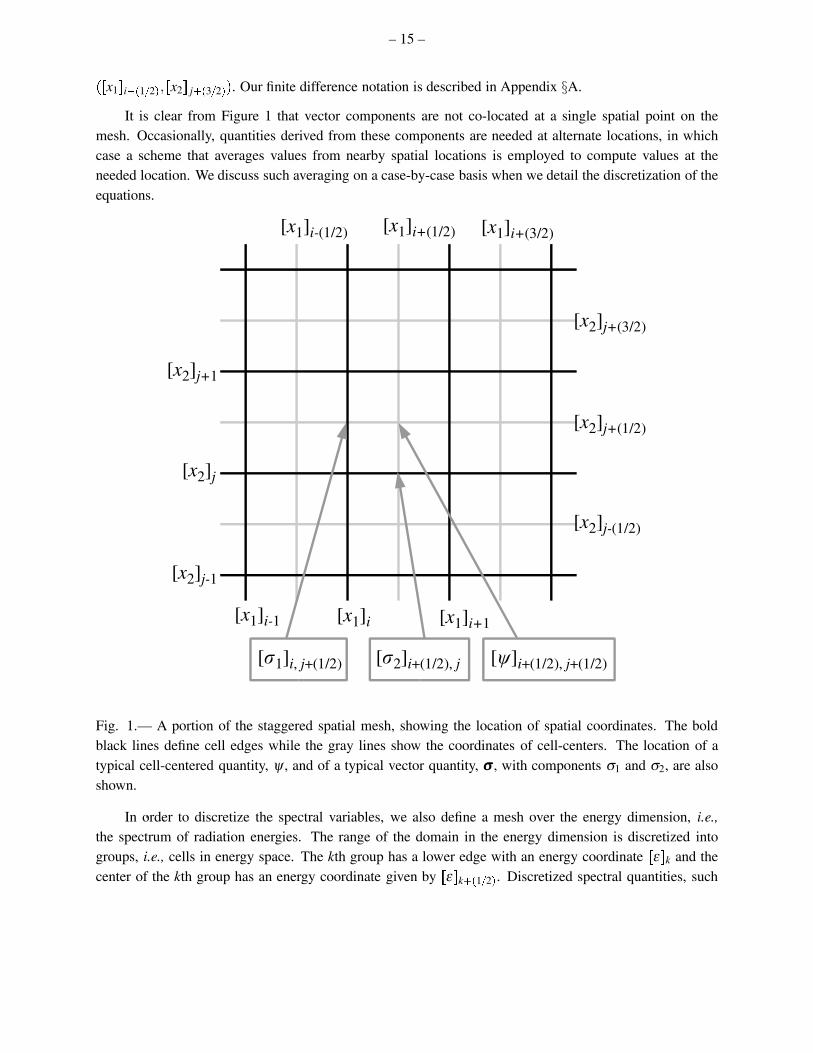

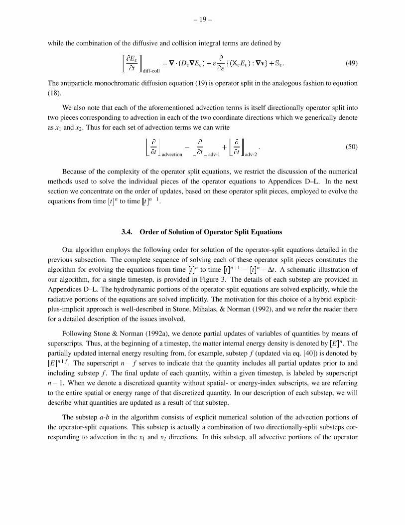

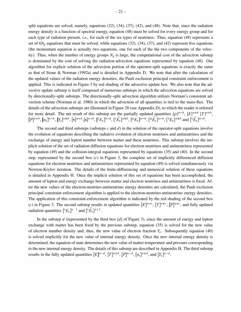
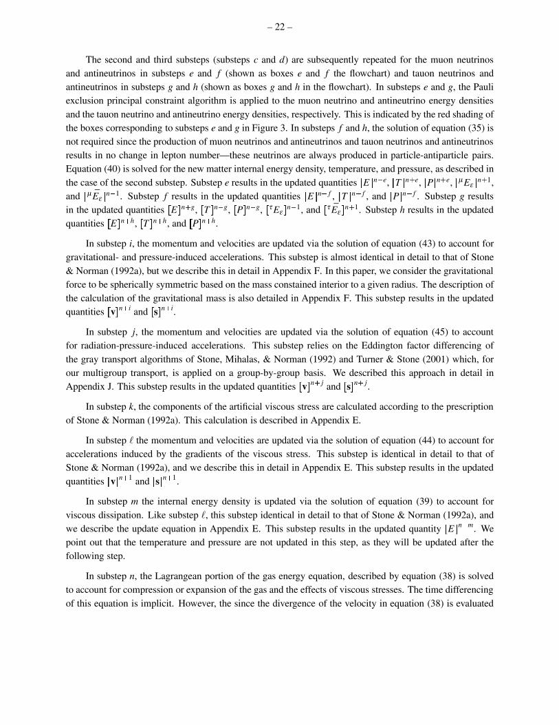
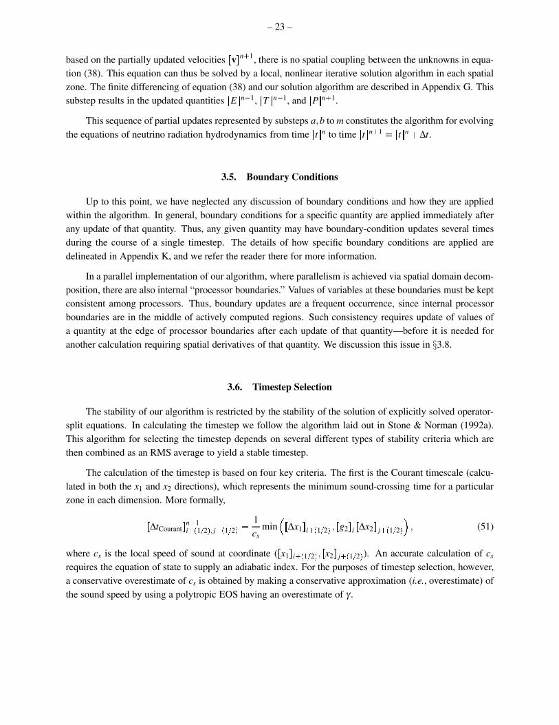

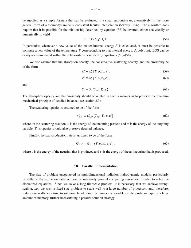
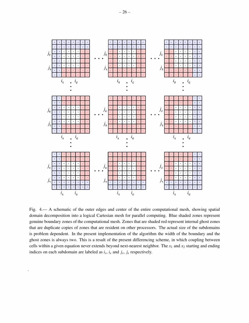

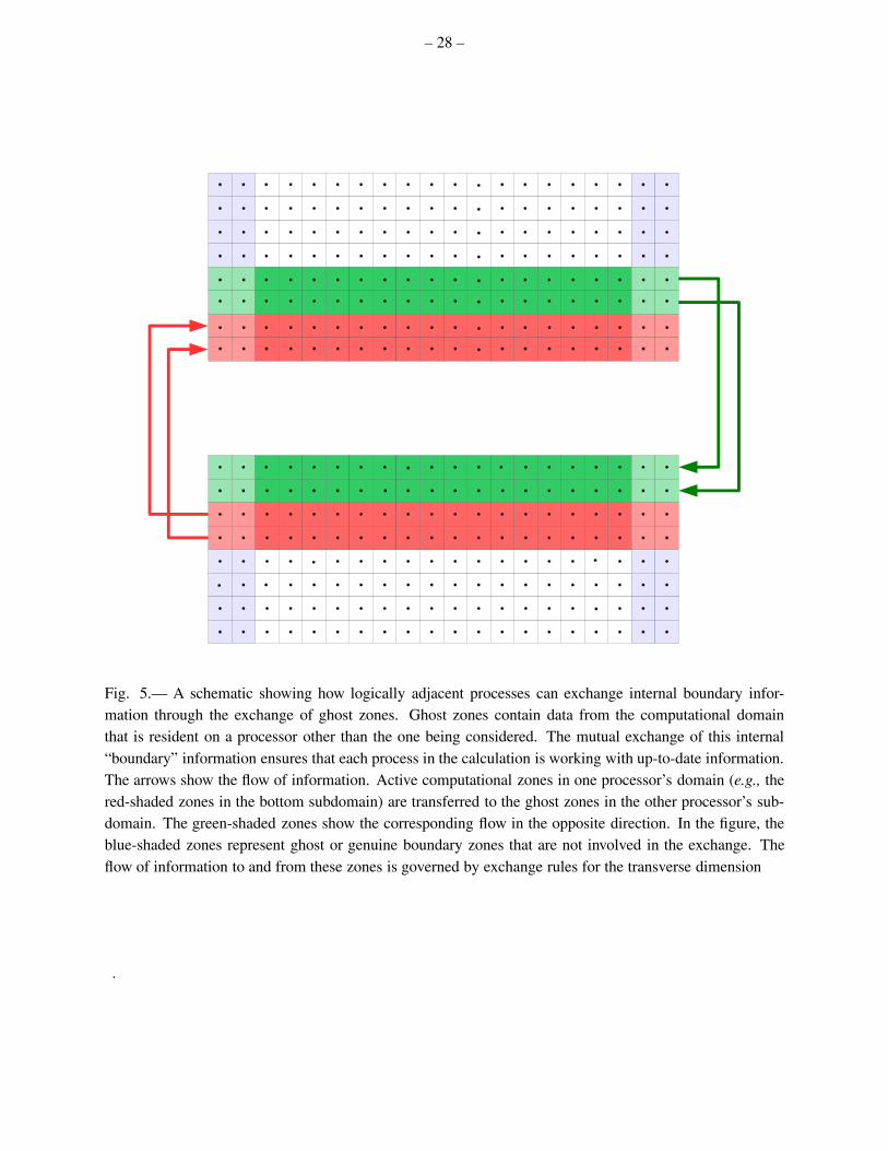
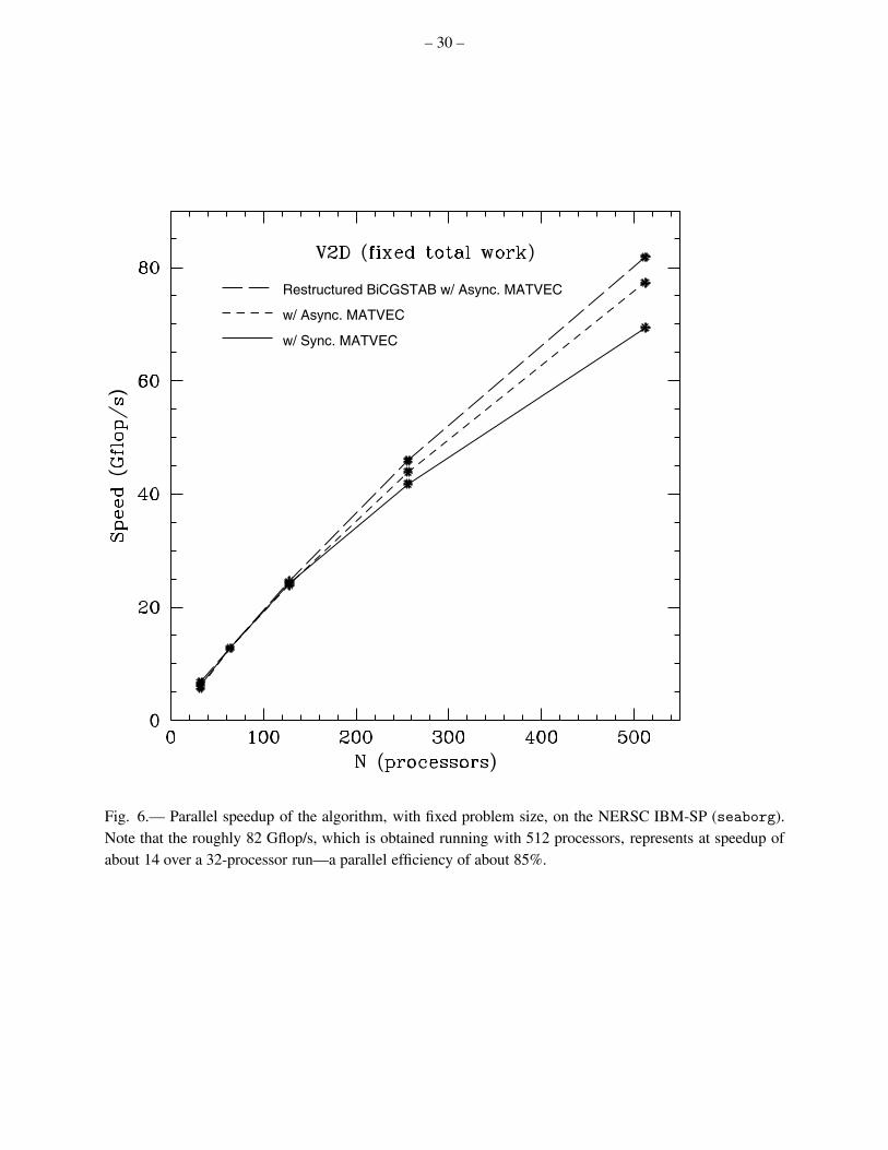
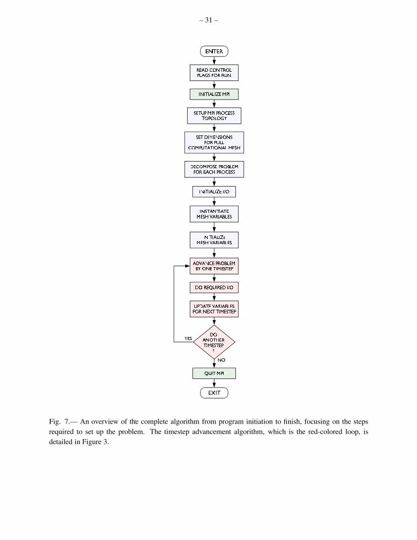


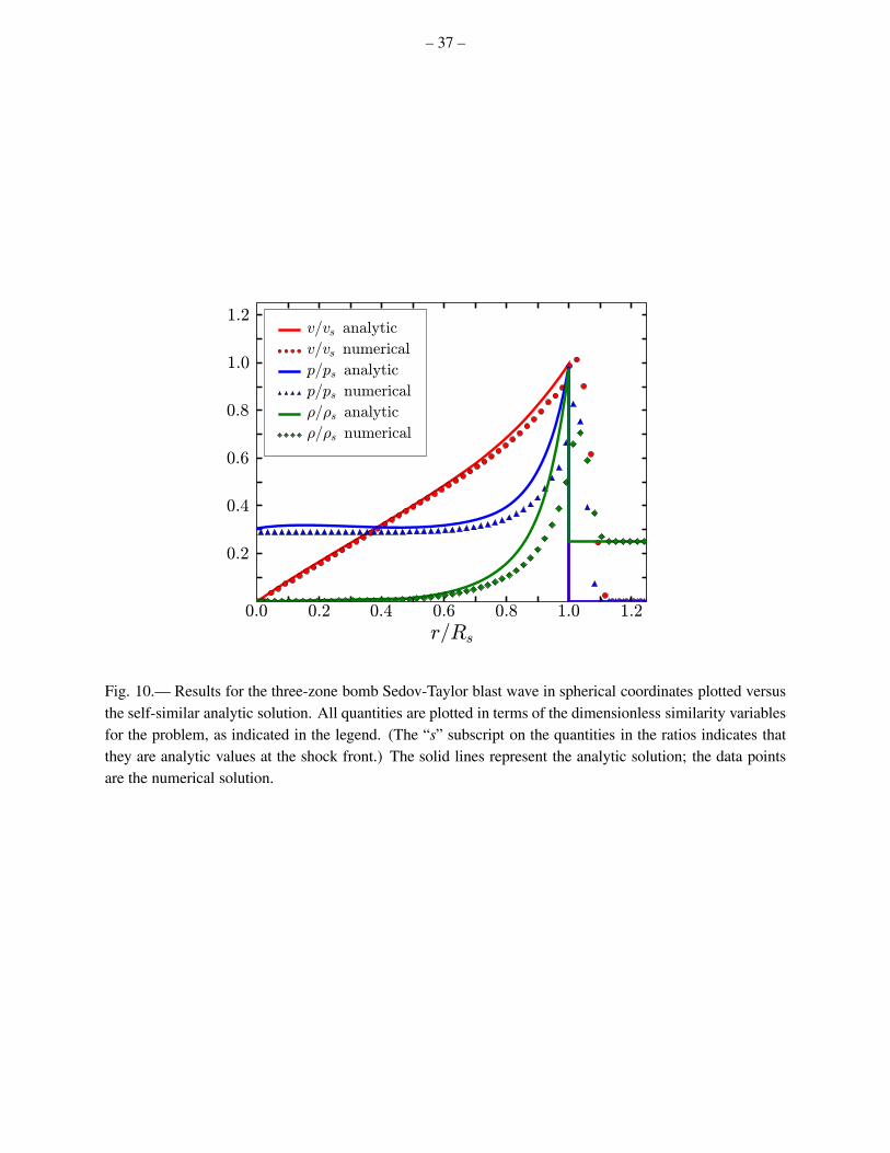

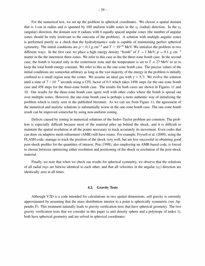


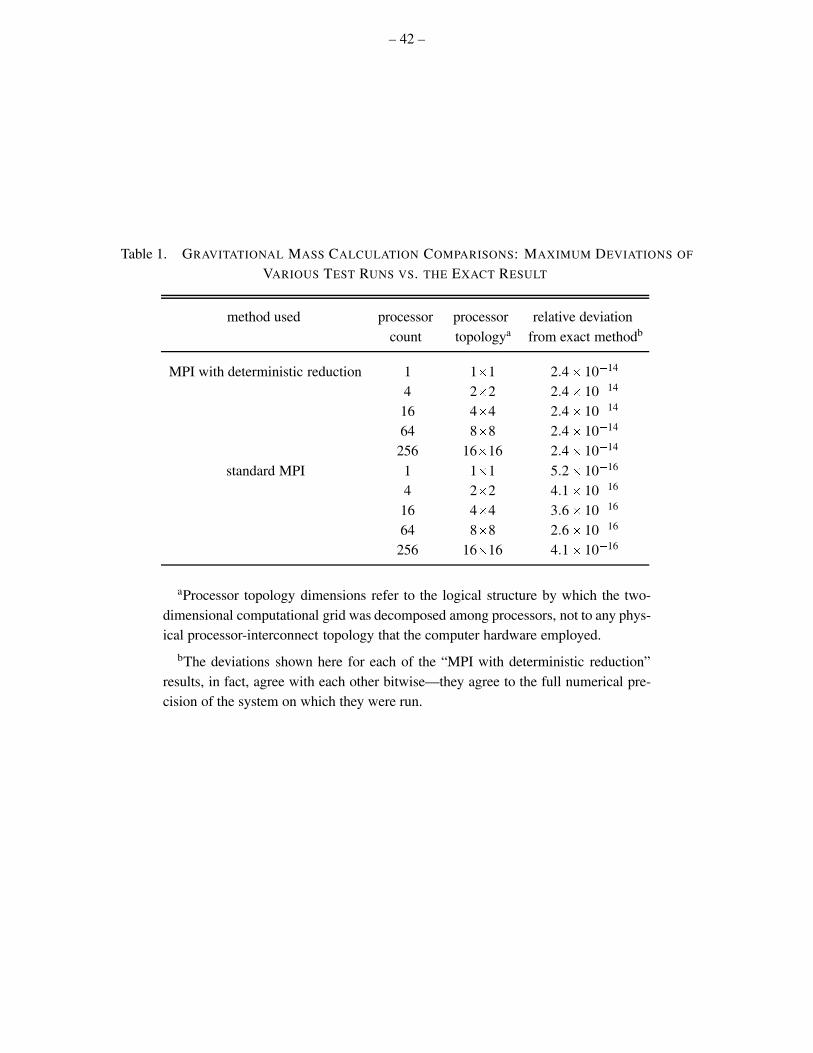


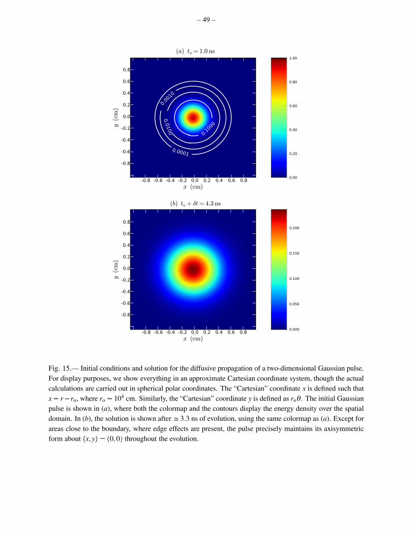
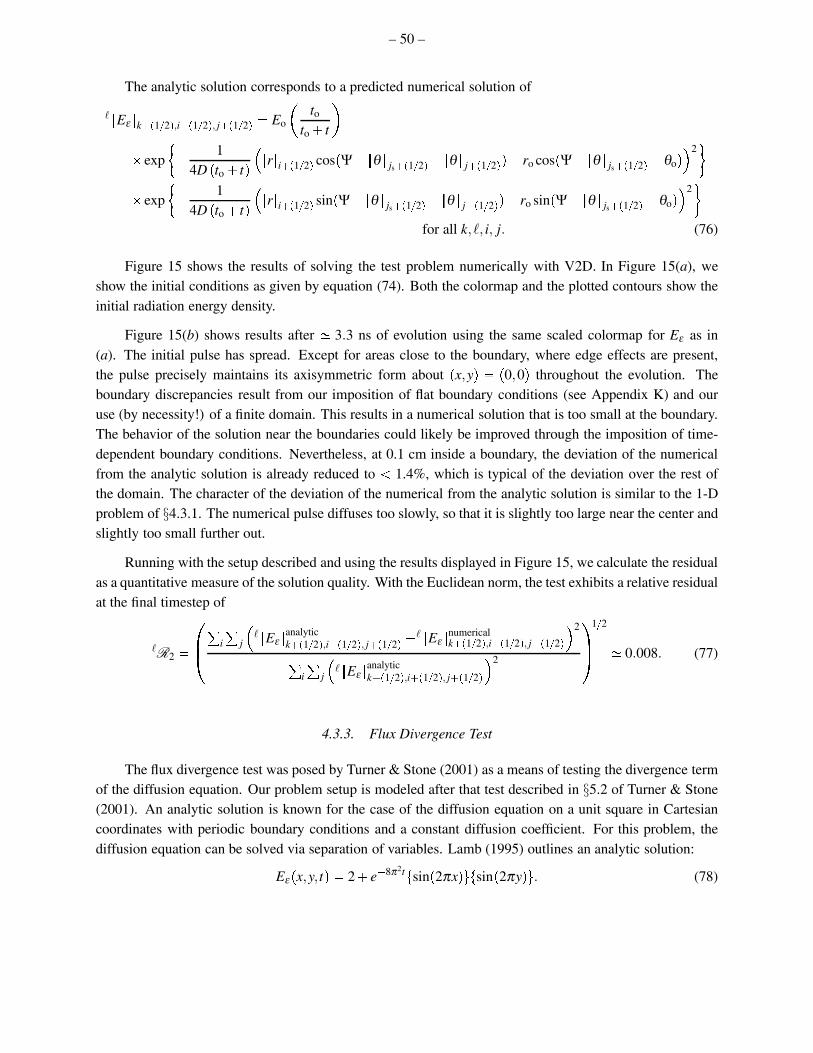


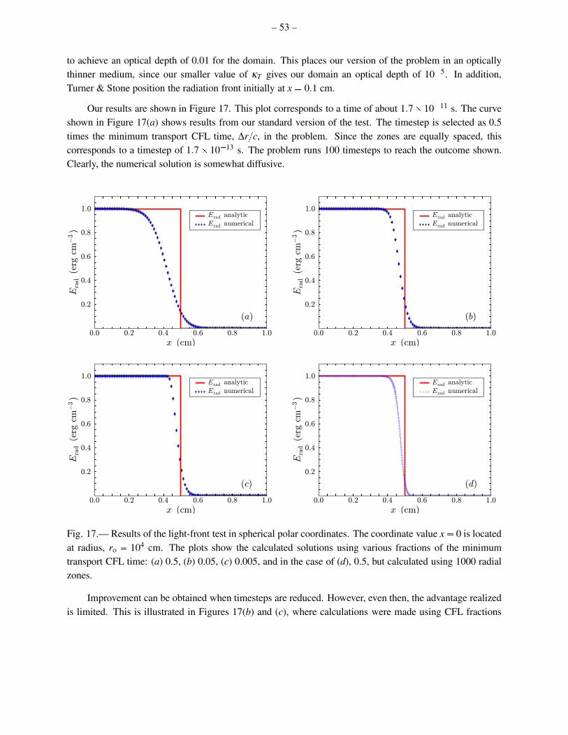

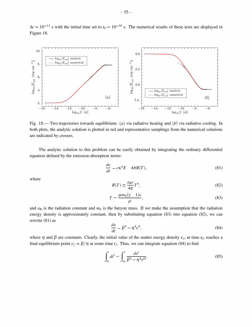


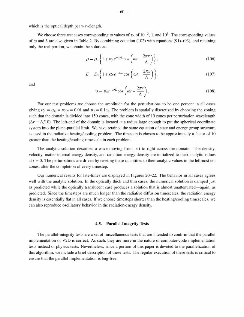


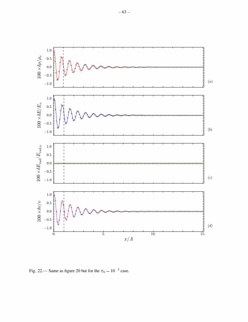
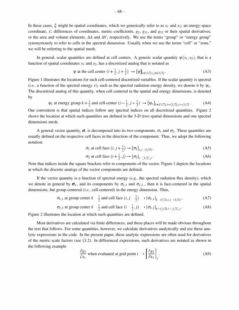

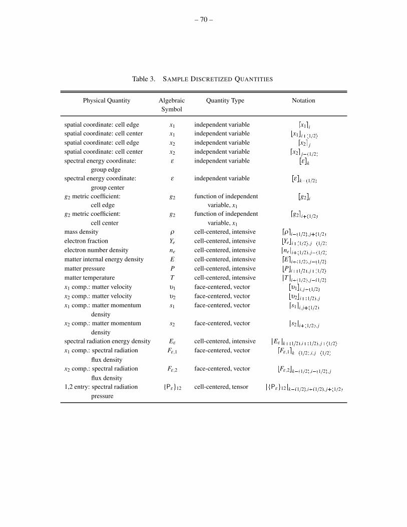
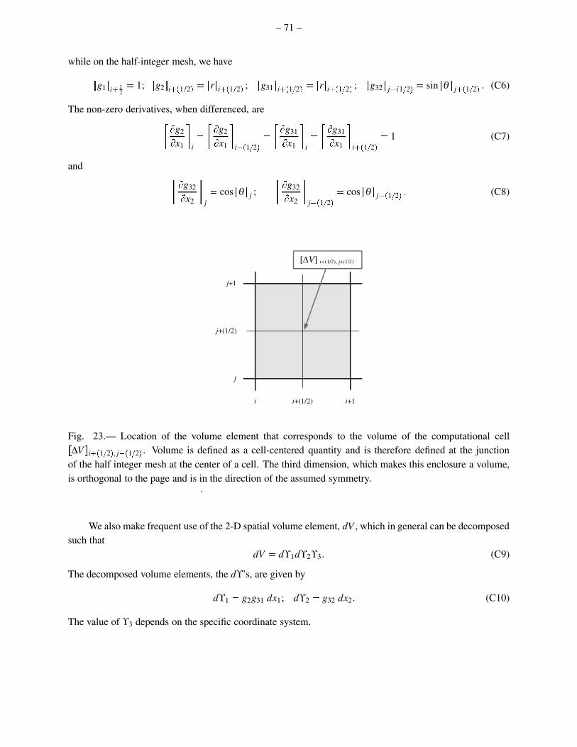
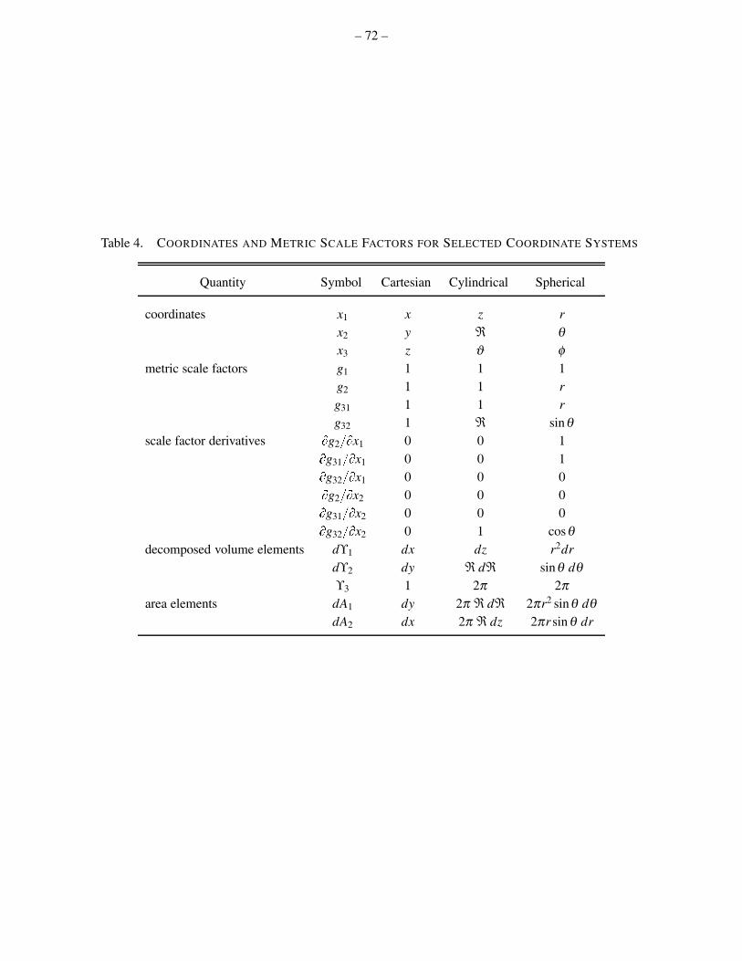


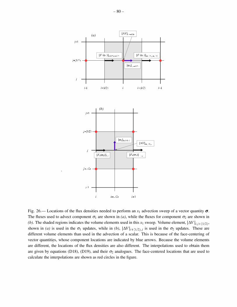


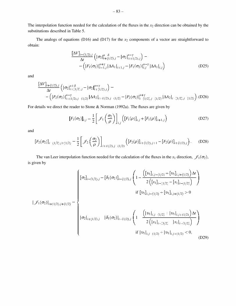


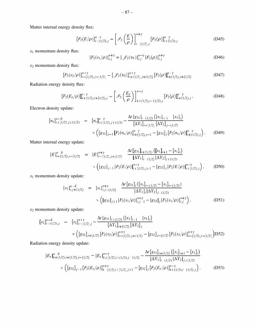


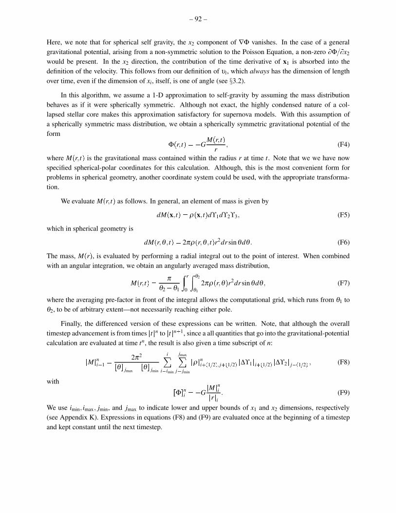


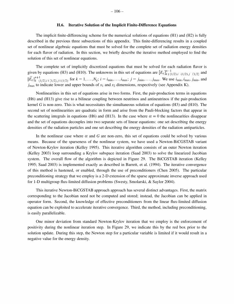


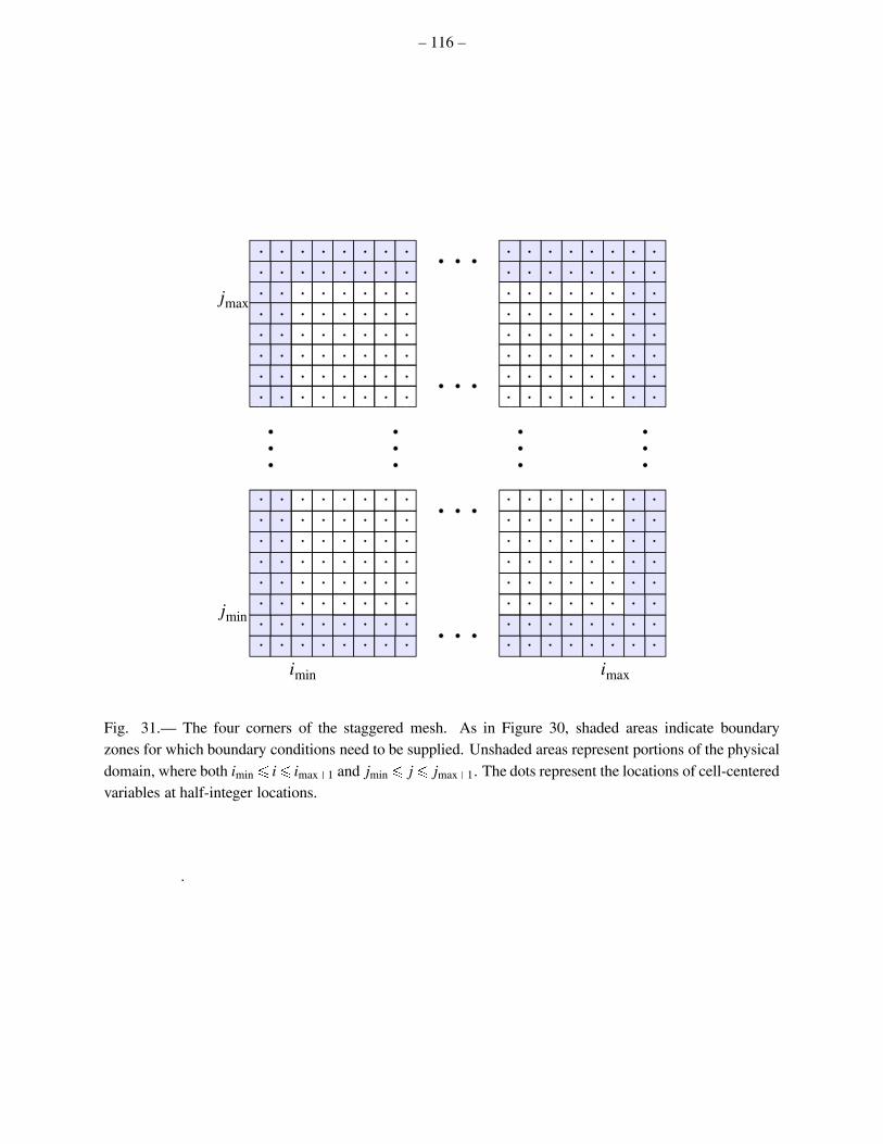


![Reactor Physics: Multigroup Diffusion · Reactor Physics: Multigroup Diffusion 6 This work is detailed in [GARLAND1975] but for the present discussion, the main point to note is the](https://static.documents.pub/doc/80x56/5e38d3c86fdaec5c757d1316/reactor-physics-multigroup-reactor-physics-multigroup-diffusion-6-this-work-is.jpg)


