Tilburg University Mixture multigroup factor analysis for ...

Tilburg University

Mixture multigroup factor analysis for unraveling factor loading noninvariance acrossmany groupsDe Roover, Kim; Vermunt, Jeroen K.; Ceulemans, Eva

Published in:Psychological Methods

DOI:10.1037/met0000355

Publication date:2022

Document VersionPeer reviewed version

Link to publication in Tilburg University Research Portal

Citation for published version (APA):De Roover, K., Vermunt, J. K., & Ceulemans, E. (2022). Mixture multigroup factor analysis for unraveling factorloading noninvariance across many groups. Psychological Methods. https://doi.org/10.1037/met0000355

General rightsCopyright and moral rights for the publications made accessible in the public portal are retained by the authors and/or other copyright ownersand it is a condition of accessing publications that users recognise and abide by the legal requirements associated with these rights.

• Users may download and print one copy of any publication from the public portal for the purpose of private study or research. • You may not further distribute the material or use it for any profit-making activity or commercial gain • You may freely distribute the URL identifying the publication in the public portal

Take down policyIf you believe that this document breaches copyright please contact us providing details, and we will remove access to the work immediatelyand investigate your claim.

Download date: 12. Mar. 2022

https://doi.org/10.1037/met0000355

https://research.tilburguniversity.edu/en/publications/c77633e0-bfd9-4aea-8ad2-32e5df61f46b

https://doi.org/10.1037/met0000355

Running head: MIXTURE MULTIGROUP FACTOR ANALYSIS

Mixture multigroup factor analysis for unraveling factor loading non-

invariance across many groups

Kim De Roover

Tilburg University, KU Leuven

Jeroen K. Vermunt

Tilburg University

Eva Ceulemans

KU Leuven

© 2020, American Psychological Association. This paper is not the copy of record and may not exactly

replicate the final, authoritative version of the article. Please do not copy or cite without authors' permission.

The final article will be available, upon publication, via its DOI: 10.1037/met0000355

Author Notes:

The research leading to the results reported in this paper was funded by the Netherlands

Organization for Scientific Research (NWO) [Veni grant 451-16-004]. The computational

resources and services used in this work were provided by the VSC (Flemish Supercomputer

Center), funded by the Research Foundation - Flanders (FWO) and the Flemish Government –

department EWI. We thank Batja Mesquita (KU Leuven) for allowing us to re-analyse the

emotional acculturation data. A preliminary version of the research results reported in this paper

were previously presented at IMPS 2018 and a preprint of the manuscript was posted on

researchgate.net and psyarxiv.com (De Roover, Vermunt, & Ceulemans, 2019). Correspondence

concerning this paper should be addressed to Kim De Roover, Tilburg School of Social and

Behavioral Sciences, Department of Methodology and Statistics, PO box 90153 5000 LE Tilburg,

The Netherlands. E-mail: [email protected].

MIXTURE MULTIGROUP FACTOR ANALYSIS 2

Abstract

Psychological research often builds on between-group comparisons of (measurements of)

latent variables; for instance, to evaluate cross-cultural differences in neuroticism or mindfulness.

A critical assumption in such comparative research is that the same latent variable(s) are measured

in exactly the same way across all groups (i.e., measurement invariance). Otherwise, one would

be comparing apples and oranges. Nowadays, measurement invariance is often tested across a large

number of groups by means of multigroup factor analysis. When the assumption is untenable, one

may compare group-specific measurement models to pinpoint sources of non-invariance, but the

number of pairwise comparisons exponentially increases with the number of groups. This makes

it hard to unravel invariances from non-invariances and for which groups they apply, and it elevates

the chances of falsely detecting non-invariance. An intuitive solution is clustering the groups into

a few clusters based on the measurement model parameters. Therefore, we present mixture

multigroup factor analysis (MMG-FA) which clusters the groups according to a specific level of

measurement invariance. Specifically, in this paper, clusters of groups with metric invariance (i.e.,

equal factor loadings) are obtained by making the loadings cluster-specific, whereas other

parameters (i.e., intercepts, factor (co)variances, residual variances) are still allowed to differ

between groups within a cluster. MMG-FA was found to perform well in an extensive simulation

study, but a larger sample size within groups is required for recovering more subtle loading

differences. Its empirical value is illustrated for data on the social value of emotions and data on

emotional acculturation.

Keywords: Measurement invariance, multigroup factor analysis, metric invariance, factor loading

invariance, mixture modeling.


1. Introduction

In psychological research, one often measures latent variables (e.g., personality traits,

attitudes) for several groups in order to evaluate between-group differences therein. A few

examples are gender differences in neuroticism (Lynn & Martin, 1997), or cross-cultural

differences in mindfulness (Christopher, Charoensuk, Gilbert, Neary, & Pearce, 2009). A critical

assumption in such comparative research is that the same latent variable(s) are measured in exactly

the same way across all groups. Otherwise, comparing the latent variables across groups would be

like comparing apples and oranges (Chen, 2008; Greiff, & Scherer, 2018). This assumption is

referred to as ‘measurement invariance’ (MI) or ‘measurement equivalence’ (Meredith, 1993).

Specifically, how the latent variables are measured by, for instance, questionnaire items is

expressed by the so-called ‘measurement model’ (MM), indicating which items measure which

latent variables, and this MM needs to be invariant across groups.

The MM is traditionally evaluated with item response theory (IRT; De Ayala, 2013) in case

of dichotomous or ordinal items, and with factor analysis (Lawley & Maxwell, 1962) when the

items are considered to be continuous. In this paper, we focus on factor analysis, where the so-

called ‘factors’ ideally correspond to the latent variables of interest. The extent to which an item

relates to a factor is quantified by a ‘factor loading’. When one wants to impose a priori

assumptions about which items are measuring which factors (by fixing certain loadings to zero)

and evaluate the fit of this MM for the data at hand, confirmatory factor analysis (CFA) is used.

In contrast, when one wants to explore whether and how the intended latent variables are measured

by the items, exploratory factor analysis (EFA) is used. Regardless of the MM being evaluated

with CFA or EFA, measurement invariance pertains to the equality (i.e., invariance) of certain

parameters of the factor model across all groups. The tenability of this invariance is tested by


means of multigroup factor analysis (MG-FA; Dolan, Oort, Stoel, & Wicherts, 2009; Jöreskog,

1971; Sörbom, 1974) with a sequence of progressively more restricted models (see Section 2 for

more details). Specifically, in multigroup CFA, one starts by inspecting model fit in order to

evaluate ‘configural invariance’, that is, whether the number of factors and the imposed pattern of

zero loadings holds across the groups (Meredith, 1993). In multigroup EFA, no specific zero

loadings are imposed. Next, in both approaches, the tenability of ‘weak’ or ‘metric invariance’ is

evaluated by restricting the factor loadings to be equal across groups. When metric invariance

holds, latent structures (e.g., how neuroticism affects another latent variable) are comparable

across groups. Subsequently, ‘strong’ or ‘scalar invariance’ is tested by also restricting the item

intercepts to be equal across groups. The finding of scalar invariance is a prerequisite for the

between-group comparability of latent means (e.g., the mean level of neuroticism). Finally, ‘strict

invariance’ or invariance of uniquenesses pertains to the equality of the residual or ‘unique’

variances of the items across groups. When combined with equal factor variances, this is a test of

the equivalence of item reliability across groups (Vandenberg & Lance, 2000). Each level of

invariance is tested by inspecting whether model fit drops significantly when the relevant MM

parameters are restricted to be equal across groups (Cheung & Rensvold, 2002).

When a certain level of MI is rejected across groups, one may resort to pairwise

comparisons of group-specific MM parameters in an attempt to pinpoint sources of non-invariance

– i.e., which parameters are non-invariant for which groups? – and figure out how to move forward.

However, the number of pairwise comparisons of group-specific parameters exponentially

increases as the number of groups increases and, nowadays, the number of groups involved is on

the rise (Kim, Cao, Wang, & Nguyen, 2017; Rutkowski & Svetina, 2014). The growing abundance

of large-scale cross-national surveys such as the World Values Survey, European Social Survey,


and International Social Survey Programme exemplify this trend. This poses two important

problems (Byrne & van de Vijver, 2010; Rutkowski & Svetina, 2014): Firstly, the multitude of

comparisons makes it hard to disentangle invariant and non-invariant parameters and for which

groups they apply. Secondly, it elevates the chances of falsely detecting non-invariance with

hypothesis testing. Therefore, after the hard work of collecting data from many groups, researchers

often cannot proceed with the comparisons of interest, at least not without risking invalid results.

Though, theoretically, each group may have its own MM, realistically, some groups are

likely to have the same measurement parameters. Therefore, a few clusters of groups may emerge

with respect to these parameters. To capture these clusters, we present a new method called

‘mixture multigroup factor analysis’ (MMG-FA), which is an extension of multigroup factor

analysis that performs a mixture clustering (McLachlan & Peel, 2000) of the groups based on (a

specific subset of) the MM parameters, whereas other parameters remain group-specific.

Specifically, to tackle metric (non-)invariance, the current paper focuses on a variant of MMG-FA

that clusters the groups purely on their factor loadings, whereas parameters irrelevant for metric

invariance are estimated per group. Thus, irrespective of other parameter differences, groups with

(near-)identical factor loadings end up in the same mixture cluster and are modeled with one set

of cluster-specific factor loadings. Clustering groups based on their MM parameters – i.e., factor

loadings in this case – not only confines the number of comparisons needed to identify sources of

non-invariance, the clustering of the countries is an interesting result in itself. Firstly, it indicates

for which groups metric invariance holds. Secondly, the clustering may indicate substantively

interesting between-group differences, for instance, cross-cultural differences in the functioning

of a questionnaire item or in the latent variables measured by the items. Obviously, the mixture

clustering of groups introduces an important model selection problem, i.e., the user needs to


determine the most appropriate number of clusters for a given data set. A solution for this model

selection problem is discussed and evaluated in this paper.

In the literature, several methods have been proposed to evaluate measurement (non-

)invariance for many groups, but MMG-FA differs from them in two important respects. Firstly,

the existing methods are predominantly CFA-based – for an overview, see Kim et al. (2017) –

whereas EFA has some important advantages when it comes to evaluating MI (Marsh, Morin,

Parker, & Kaur, 2014): Firstly, assumed MMs often do not hold or not for all groups (i.e.,

configural invariance fails). In that case, respecifying CFA models in an exploratory way

capitalizes on chance (Browne, 2001; MacCallum, Roznowski, & Necowitz, 1992) and using EFA

right from the start is the better strategy (Gerbing & Hamilton, 1996). Secondly, even when the

MM holds, fixed zero loadings are often too restrictive (Asparouhov & Muthén, 2009; Muthén &

Asparouhov, 2012). For instance, for the well-known Big five model of personality, it was shown

that zero loadings are untenable (McCrae, Zonderman, Costa, Bond, & Paunonen, 1996). Thirdly,

model misspecifications can severely bias the estimates of other MM parameters, such as the other

loadings (Anderson & Gerbing, 1982; Bollen, Kirby, Curran, Paxton, & Chen, 2007), and may

differ across groups (e.g., Byrne & van de Vijver, 2010; Christopher, Charoensuk, Gilbert, Neary,

& Pearce, 2009). For all these reasons and to prevent the clustering from being affected by model

misspecifications, MMG-FA applies EFA for estimating the cluster-specific factor loadings. As a

result, MMG-FA simultaneously models differences in the pattern of (near-)zero and non-zero

loadings as well as differences in the strength of the non-zero loadings (i.e., both configural and

metric non-invariances).

Secondly, some existing CFA-based (Kim et al., 2017) and EFA-based (De Roover,

Vermunt, Timmerman, & Ceulemans, 2017) methods apply a mixture approach similar to MMG-


FA, but neither of them clusters the groups exclusively on specific subsets of the MM parameters.

The latter is an important step forward as MI is traditionally evaluated in a stepwise manner, where

different levels of (non-)invariance have different implications in terms of which comparisons are

(in)valid (Meredith, 1993). To allow for substantive researchers to focus on the level of invariance

they need for a particular research question or to scrutinize non-invariances in a stepwise manner,

MMG-FA clusters groups based on their MM parameters in a level-specific way, where metric

invariance is the focus of this paper. Metric invariance is sufficient for studies where the

comparability of latent structures is of interest rather than comparing latent means (e.g., Byrne,

Baron, & Balev, 1998; Byrne & Shavelson, 1986; Cooke, Kosson, & Michie, 2001; Marsh, Hau,

Artelt, Baumert, & Peschar, 2006). Suggestions on how to continue towards higher levels of MI

are given in the Discussion. Note that clustering the groups based on all MM parameters at the

same time (i.e., also on intercepts and unique variances) would imply the rather stringent

assumption that one clustering is underlying all MM parameters, whereas some parameter

differences may be explained by another clustering – possibly with a higher number of clusters –

or they may be group-specific. When this assumption does not hold, the obtained clustering may

even fail to capture the underlying factor loading differences. For the same reason, MMG-FA also

sets aside so-called ‘structural’ parameters that are irrelevant to the MI question – such as

differences in factor (co)variances. Surely, when clustering groups in terms of how the items of a

questionnaire measured, for instance, neuroticism and extraversion, it is irrelevant how the groups

differ with respect to the (co)variance of neuroticism and extraversion. Clustering the groups based

on a specific subset of MM parameters also limits the number of parameter comparisons needed

to untangle what is different between which clusters, which adds to the insightfulness and


efficiency of the method and again lowers the risk of false positives when performing hypothesis

tests for parameter differences.

The remainder of this paper is organized as follows: Section 2 recaps MG-FA and discusses

its extension into MMG-FA, covering details about model specification, model estimation and

model selection. Section 3 describes an extensive simulation study to evaluate the performance of

MMG-FA in terms of model estimation and model selection. Section 4 illustrates the added value

of MMG-FA for cross-cultural data sets on the social value of emotions and on emotional

acculturation. Section 5 concludes with some points of discussion and directions for future

research.

2. Method

2.1. Multigroup factor analysis

Multigroup factor analysis (MG-FA; Jöreskog, 1971; Sörbom, 1974) operates on data from

multiple groups (e.g., patient groups, countries). The groups are indicated by g = 1, …, G and the

subjects by gn = 1, …, Ng. The scores for subject

gn on the J items are denoted by the vector gnx

and, per group g, they are gathered in an Ng × J matrix Xg. The factor model for gnx is written as:

g g gn g g n n x τ Λ η ε (1)

where gτ indicates a J-dimensional group-specific intercept vector,

gΛ denotes a J × Q matrix of

group-specific factor loadings,gnη is a Q-dimensional vector of scores on the Q factors and

gnε is a

J-dimensional vector of residuals. The factor loadings indicate the linear item-factor associations.

The factor scores indicate how subject gn scores on the latent variables and are assumed to be


identically and independently distributed (i.i.d.) as ,g gMVN α Φ , independently of gnε , which

are i.i.d. as , gMVN 0 Ψ . The factor means of group g are denoted by gα , whereas

gΦ pertains

to the factor (co)variances and gΨ to a diagonal matrix containing the residual or unique variances

of the items in group g. The model-implied covariance matrix for group g is g g g g g

Λ Φ Λ Ψ

. In multigroup EFA (MG-EFA; Dolan, Oort, Stoel, & Wicherts, 2009), the group-specific factors

have rotational freedom which is dealt with by a rotation criterion (De Roover & Vermunt, 2019).

Estimating Equation 1 per group corresponds to the baseline model for MI testing. To

partially identify the model, the factor means gα are fixed to zero and the factor covariance matrix

gΦ to identity (i.e., orthonormal factors: uncorrelated with variances equal to one) per group g.

That fact that MG-EFA does not impose specific zero loadings on gΛ makes it more flexible than

multigroup CFA (MG-CFA; Meredith, & Teresi, 2006; Sörbom, 1974) in terms of the factor

loading differences that can be found (De Roover & Vermunt, 2019). MI is tested by the following

sequence of progressively more restricted models (Cheung & Rensvold, 2002; Dolan et al., 2009).

Weak or metric invariance is evaluated by comparing the fit of the baseline model and the model

with invariant loadings, i.e., g Λ Λ for g = 1, …, G. For the latter model, orthonormality of the

factors is no longer imposed per group but, e.g., for the mean factor (co)variances across groups;

1

1 G

g g

g

NN

Φ I where I refers to a Q × Q identity matrix. Strong or scalar invariance is tested by

also restricting the intercepts gτ to be equal across groups, while freely estimating factor means

gα for all groups but one. Strict invariance is assessed by restricting the unique variances, i.e., the

diagonal of gΨ , to be the same across groups. Several criteria are available to evaluate whether a


drop in fit when moving towards a more restricted model is statistically or practically significant.

Since ² - difference tests for nested models are strongly affected by sample size, we focus on

other fit indices such as the CFI and RMSEA. Lack of invariance is indicated when the decrease

in CFI (CFI) is larger than .01 and the increase in RMSEA ( RMSEA) exceeds .01 when

imposing invariant MM parameters (Chen, 2007; Cheung & Rensvold, 2002). However, for

detecting metric non-invariance across many groups, more liberal cut-off values should be used,

i.e., CFI < –.02 and RMSEA > .03 (Rutkowski & Svetina, 2014).

In case of metric non-invariance – the focus of this paper – one can return to the baseline

model and compare group-specific loadings to locate non-invariances (e.g., De Roover &

Vermunt, 2019), but this becomes infeasible and problematic when more than a few groups are

involved (see Introduction). For instance, comparing factor loadings for five groups implies only

10 pairwise comparisons, but 10 groups require 45 comparisons and 47 groups (as in the empirical

example; Section 4) result in 1,081 comparisons. To tie down the number of comparisons needed

to identify non-invariances, we present mixture multigroup factor analysis.

2.2. Mixture multigroup factor analysis

2.2.1. Model specification

Mixture multigroup factor analysis (MMG-FA) aims to gather groups into a few clusters

according to the equivalence of their MM parameters; specifically, their factor loadings. To this

end, the observations gnx are assumed to be sampled from a mixture of K multivariate normal

distributions where all observations of a group are assumed to be sampled from the same normal

distribution. Thus, the mixture clustering operates at the group level, which is an important

difference from the well-known factor mixture modeling (Lubke & Muthén, 2005). In the


remainder of the paper, the K mixture components will be referred to as ‘clusters’. Formally, the

MMG-FA model for group g is written as follows:

1 1 1

; ; ( ; )g

g

g

NK K

g k gk g gk k n g gk gk k gk k g

k k n

f f MVN with

X X x μ Λ Φ Λ Ψ (2)

where f is the total population density function, and θ refers to the total set of parameters. The

mixing proportions (i.e., prior probabilities of a group belonging to each of the clusters) are

indicated by k , with 1

1K

k

k

, whereas fgk refers to the kth cluster-specific density function for

group g and θgk to the corresponding set of parameters. It is important to note that the means are

group-specific and the covariance matrices are both group- and cluster-specific. A combination of

group- and cluster-specific parameters is applied such that the clustering of the groups is driven

exclusively by the parameters relevant to metric invariance, i.e., the factor loadings. How to deal

with higher levels of MI is described in the Discussion. Specifically, the covariance matrices are

modeled by means of cluster-specific factor loadings kΛ , group- and cluster-specific factor

(co)variances gkΦ , and group-specific unique variances on the diagonal of

gΨ . The fact that gkΦ

is not only group-specific but also varies across clusters within groups needs some additional

explanation. Because the latent factors have a different meaning across clusters, and moreover

have rotational freedom per cluster, it is too restrictive to assume the factor (co)variances of a

group to be the same in all clusters. As shown in Appendix A, these factor (co)variances can be

estimated for every cluster despite the fact that the mixture model itself assumes that each group

belongs to only one cluster. This holds even when group g is assigned to cluster k with a probability

of zero. The resulting gkΦ should be interpreted as the factor (co)variances conditional on group


g belonging to cluster k. For each group g, the factor (co)variances for the clusters the group does

not belong to may be regarded as nuisance parameters.

Thus, in MMG-FA, the (exploratory) factor model is conditional on the cluster membership

of group g, indicated by gkz , as follows:

| 1g g gn gk g k n k nz

x τ Λ η ε (3)

where ,gn k gkMVNη 0 Φ and ,

gn gMVNε 0 Ψ . Note that, because the factor means are equal

to zero per group within each cluster, the item intercepts gτ are equal to the means

g in Equation

2. To set the scale of the cluster-specific factors, the mean factor variances are fixed to one over

all groups within a cluster k, i.e., 1

1ˆ

G

k g gk gk

gk

N zN

Φ Φ I , where1

ˆG

k g gk

g

N N z

. Note that this

restriction also fixes the factor covariances to zero over all groups within a cluster, which implies

that the initial rotation is orthogonal for each cluster. Afterwards, the cluster-specific factors can

be (orthogonally or obliquely) rotated to facilitate interpretation and comparability.

Note that the existing method that is most similar to MMG-FA, as specified above, is

mixture simultaneous factor analysis (MSFA; De Roover, Vermunt, Timmerman, & Ceulemans,

2017). Like MMG-FA – and unlike multilevel factor mixture modeling (Kim et al., 2017) – MSFA

sets apart the means as group-specific parameters and uses EFA within the clusters. This implies

that the mixture clustering is also unaffected by intercept or factor mean differences and that it is

equally flexible in the factor loading differences it can capture (i.e., both configural and metric

non-invariances). However, MSFA differs from MMG-FA in that the covariance matrix depends

entirely on the cluster, i.e., k k k k

Λ Λ Ψ . This implies that it assumes factor (co)variances and

unique variances to be the same for groups within a cluster, which is too restrictive when looking


for clusters of groups wherein metric invariance holds. Thus, the MSFA clustering also captures

between-group differences in factor (co)variances and unique variances, rendering this method

less focused on loading differences than MMG-FA.

2.2.2. Model estimation

The unknown parameters θ of the MMG-FA model are estimated by means of maximum

likelihood (ML) estimation. This involves maximizing the logarithm of the likelihood of the data:

1

1/2/211 1

1

1/2/21 1 1

1 1log log exp

22

1 1log exp ,

22

g

g g

g

g

g g

g

NG K

k n g gk n gJkg n

gk

NG K

k n g gk n gJg k n

gk

L

x μ Σ x μΣ

x μ Σ x μΣ

(4)

where gk is decomposed as specified in Equation 2. Note that obtaining the parameter estimates

by means of Newton-Raphson, Fisher scoring or Quasi-Newton optimization methods – i.e.,

methods that are used in commercial software such as Latent GOLD (Vermunt & Magidson, 2013,

2016) and Mplus (Muthén & Muthén, 2005) – is very slow due to the very large number of

parameters and very sensitive to starting values. To find the parameter estimates in a time-efficient

and stable manner, we developed an expectation-conditional maximization (ECM) algorithm (see

Appendix A) and implemented it in Matlab R2017a, R (see

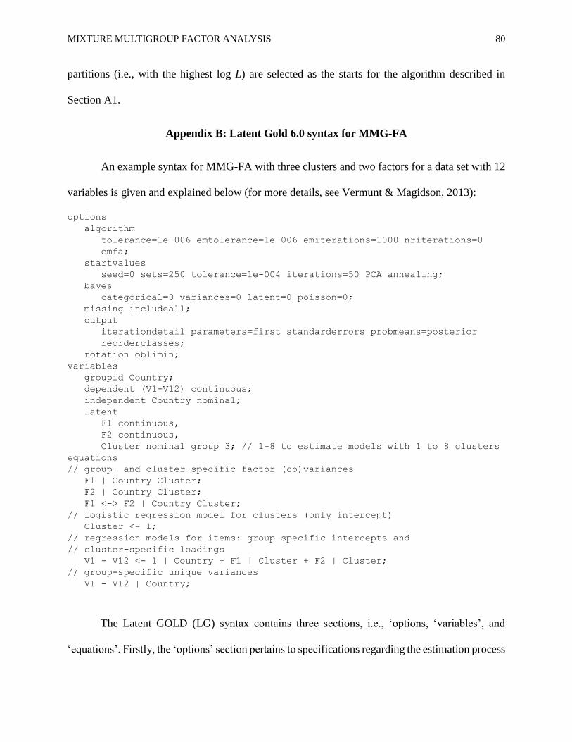
https://github.com/KimDeRoover/MixtureMG_FA), and Latent GOLD 6.0 (see Appendix B). An

R-package for MMG-FA will be developed in the near future. Because the algorithm may end up

in a local maximum, a multistart procedure (based on several random partitions of the groups or

several sets of random initial values for the parameters) is applied to increase the probability of

obtaining the global maximum (see Appendices A and B). As an indication of computation time,

the estimation of MMG-FA with three clusters and two factors for the emotion values data set


(Section 4.1) took 43 seconds with the Matlab algorithm, 188 seconds with the algorithm in R, and

160 seconds in Latent GOLD 6.0 (where the latter includes a more elaborate multistart procedure

and the computation of standard errors), when using 25 random starts (pre-selected from a set of

250 starts, see Appendices A and B). Note that repeating the same analysis in Latent GOLD

without the new ECM algorithm – thus, with Fisher scoring to estimate the factor parameters –

took more than 7 hours.

2.2.3. Model selection

In this paper, we focus on the case where the number of factors is assumed to be known

and equal for all groups, and thus for all clusters. Thus, the model selection problem is confined

to selecting the most appropriate number of clusters K for a given data set. For enumerating the

number of clusters in related mixture models, minimizing the Bayesian Information Criterion

(BIC; Schwarz 1978) is often the recommended method (Nylund, Asparouhov, & Muthén, 2007;

Tay, Diener, Drasgow, & Vermunt, 2011; Tein, Coxe, & Cham, 2013). The BIC takes into account

model complexity in addition to the log L and penalizes a model with more parameters and larger

sample size as follows:

BIC 2log log( )L fp N (5)

where fp refers to the number of free parameters and N refers to the total sample size 1

G

g

g

N

. For

MMG-FA, fp is equal to the sum of the number of mixing proportions (minus one restriction), the

cluster-specific factor loadings (corrected for rotational freedom), the factor (co)variances for each

group (minus identification restrictions), and the group-specific intercepts and unique variances:

1 ( ( 1) 2) ( ) ( 1) 2 2fp K K JQ Q Q G K Q Q GJ . Note that only one set of factor

(co)variances is counted for each group, because the remaining factor (co)variances (i.e., for the


clusters they don’t belong to) are nuisance parameters that do not contribute to the model fit (see

Section 2.2.1).

Several authors (Kim, Joo, Lee, Wang, & Stark, 2016; Lukočienė, Varriale, & Vermunt,

2010) suggested that, for group-level clusters, it is better to use the number of groups G for the

sample size in the computation of BIC instead of the number of subjects N. In case of small sample

size and low cluster separation in multilevel mixture modeling, it was found that the Akaike

Information Criterion (AIC; Akaike, 1973) outperformed the BIC (Kim et al., 2017; Lukočienė,

Varriale, & Vermunt, 2010). For growth mixture models, Bauer (2007) and McNeish and Harring

(2017) indicated that in less ideal – but empirically more realistic – conditions (e.g., non-

normality), BIC (and AIC) may overselect the number of clusters.

Finally, Bulteel, Wilderjans, Tuerlinckx, and Ceulemans (2013) showed that the Convex

Hull procedure (CHull) is a valuable alternative to BIC and AIC in the context of mixtures of

factor analyzers. The CHull (Ceulemans & Van Mechelen, 2005; Ceulemans & Kiers, 2006) is a

generalization of the scree test (Cattell, 1966). Specifically, the CHull procedure balances fit and

complexity by comparing the log L and fp of the obtained solutions and selecting the one with the

highest scree ratio. Note that, like a scree test, CHull cannot select the least complex model and

thus always selects at least two clusters. But since we are focusing on cases where factor loading

invariance was rejected, and loading differences are thus expected to be present, we don’t regard

this to be a problem. Furthermore, visual inspection of the CHull plot may still lead to the

conclusion that no clear elbow is present and thus that an underlying clustering is unlikely. How

these methods perform in terms of selecting the correct number of clusters for MMG-FA is

evaluated in Section 3.


3. Simulation Studies

In this section, we first present a large simulation study to evaluate the performance of

MMG-FA, both in terms of model estimation and model selection, when clusters of groups with

metric invariance are underlying the data. Then, a smaller simulation study is presented to evaluate

MMG-FA, specifically in terms of model selection, when no such clusters are underlying the data

and metric invariance holds across all groups (i.e., the number of clusters equals one).

3.1. Simulation Study 1

Problem.

The goal of Simulation Study 1 is, on the one hand, to evaluate the performance of MMG-

FA with respect to the recovery of the clustering of the groups and of the cluster-specific factor

loadings when the correct number of clusters is known and to compare this performance to that of

MSFA. On the other hand, it is evaluated to what extent the model selection procedures described

in Section 2.2.3 select the correct number of clusters for MMG-FA. We manipulated six factors

that were expected to affect the cluster separation and/or the stability of parameter estimates, and

thus the performance of MMG-FA and its model selection: (1) the number of groups, (2) the group

sizes, (3) the number of clusters, (4) the cluster sizes, (5) the number of factors, and (6) the type

and size of the loading differences.

Specifically, in terms of their effect, we hypothesize the following: The number of groups

(1) determines how many groups end up within each cluster. Because more groups within a cluster

implies more information on that cluster-specific MM (i.e., a higher within-cluster sample size),

we hypothesize the performance to improve with a higher number of groups. A higher number of

observations per group (2) increases the within-cluster sample size and thus the performance. It


also implies more information on each of the cluster memberships and thus a higher cluster

separation (i.e., how easy it is to distinguish the clusters from one another and determine the cluster

memberships; Lukočienė, Varriale, & Vermunt, 2010). Relatedly, a higher number of clusters (3)

lowers the within-cluster sample size (for a given number of groups) and is thus expected to lower

the performance. It also increases the number of cluster memberships (posterior probabilities) to

be determined for each group and thus makes their recovery more intricate. The cluster sizes (4),

corresponding to the mixing proportions, pertain to the groups being equally or unequally divided

across the clusters. In the unequal case, larger cluster(s) will compete with smaller cluster(s) and

the smaller ones will be much harder to recover both in terms of cluster memberships and factor

loading estimates. With respect to the number of factors (5), a higher number of factors – given

the same number of variables – implies a lower factor overdetermination and thus probably a lower

performance. Finally, the type and size of loading differences (6) greatly determines the extent to

which the cluster-specific MMs differ from one another (i.e., cluster separation) and thus affects

the recovery of the cluster memberships. For instance, a primary loading that shifts to another

factor is a large difference that would be easier to recover than a small difference in the size of a

primary loading or crossloading.

Design.

These factors were systematically varied in a complete factorial design:

1. the number of groups G at 2 levels: 12, 60;

2. the group sizes Ng (i.e., number of observations per group) at 5 levels: 30, 50, 100, 300,

500;

3. the number of clusters K at 2 levels: 2, 4;

4. the cluster sizes at 2 levels: equal, unequal;

5. the number of factors Q at 2 levels: 2, 4;


6. the type and size of loading differences at 5 levels: primary loading shift, crossloading of

.40, crossloading of .20, primary loading decrease of .40, primary loading decrease of .20.

The number of variables J was fixed at 20 and the cluster-specific factor loading matrices

were generated by inducing changes to the same simple structure loading matrix. In this ‘base

loading matrix’, the variables are equally distributed over the factors, i.e., each factor gets 10 non-

zero loadings when Q = 2 (Table 1) and five non-zero loadings when Q = 4 (Table 2). Given that

the unique variances vary around .40 (see below), the non-zero loadings are equal to .60 to

obtain total variances that vary around one. From the common base, K different cluster-specific

loading matrices are derived by altering the loadings for a different pair of variables for each cluster

(see Tables 1 and 2). Specifically, depending on the type and size of loading differences, the

loadings of two variables were altered as follows: In case of a primary loading shift, when Q = 2,

the loadings .6 0 of the base matrix are replaced by 0 .6

or vice versa (Table 1). When Q

= 4, primary loadings are shifted similarly between factors 1 and 2, leaving factors 3 and 4

unaffected; e.g., .6 0 0 0 becomes 0 .6 0 0

. In case of the crossloading differences, the

loadings .6 0 0 0 become .6 .4 0 0

or .6 .2 0 0 depending on the size of

the crossloadings (Table 2). Note that a crossloading of .20 may be considered ‘ignorable’, whereas

one of .40 is not (Stevens, 1992). To manipulate a primary loading decrease, the loadings

.6 0 0 0 are replaced by .6 .4 0 0 0

or .6 .2 0 0 0 depending on the size

of the decrease (Table 3). A primary loading decrease of .40 is considered a large non-invariance

(Stark, Chernyshenko, & Drasgow, 2006) that can lead to incorrect statistical inference and biased

parameter estimates (Hancock, Lawrence, & Nevitt, 2000). Please observe the following: Firstly,

a primary loading shift maintains the item’s communality whereas a crossloading increases it and


a primary loading decrease lowers it. Secondly, primary loading shifts and crossloadings are

violations of configural invariance and thus differences that are very hard to trace by any of the

existing CFA-based methods (Kim et al., 2017).

[ Insert Tables 1 to 3 about here ]

Note that the number of groups of 12 and 60 nicely correspond to the range of group

numbers that are generally encountered in large-scale surveys (Rutkowski & Svetina, 2014). In

case of equal cluster sizes, the groups are equally divided across the clusters, i.e., each cluster

contains 50% of the groups in case of two clusters or 25% in case of four clusters. In the unequal

cluster size conditions, the groups are divided over the clusters such that one cluster contains 75%

of the groups, whereas the remaining groups are equally divided over the other clusters. Thus, in

case of two clusters, 75% of the groups are in one cluster and 25% in the other one. In case of four

clusters, each of the three smaller clusters contains 8.33% of the groups. Note that the latter

correspond to singleton clusters (i.e., including only one group) in case of 12 groups, whereas in

case of 60 groups they hold five groups each. The cluster memberships were generated by

randomly assigning the correct number of groups to each cluster, according to these cluster sizes.

The group- and cluster-specific factor correlations are randomly sampled from a uniform

distribution between −.50 and .50, i.e., .50,.50U , and factor variances from .50,1.50U .

Whenever a resulting gkΦ is not positive definite, the sampling is repeated. Group-specific unique

variances (i.e., diagonal of gΨ ) are sampled from .20,.60U . Factor scores are sampled from

, gkMVN 0 Φ and residuals from , gMVN 0 Ψ , according to the specified group sizes. The group

size of 100 corresponds to the absolute minimal sample size for obtaining accurate factor loading

estimates (Gorsuch, 1983), whereas higher sample sizes are recommended in case of lower factor


overdetermination and/or item communalities (Fabrigar, MacCallum, Wegener, & Strahan, 1999;

MacCallum, Widaman, Zhang, & Hong, 1999). Note that, for MMG-FA, the accuracy of the factor

loadings will be determined by the sample size of a cluster of groups, rather than of a single group,

whereas the accuracy of the factor (co)variances of groups within a cluster may depend on the

group sizes. To evaluate the extent to which MMG-FA can find loading differences among really

small groups, we included the group sizes of 30 and 50. Finally, the simulated data are created

according to Equation 3. The intercepts gτ are zero, since the focus is on loading differences.

According to this procedure, 50 data sets were generated per cell of the design, using

Matlab R2017a. Thus, 2 (number of groups) × 5 (group sizes) × 2 (number of clusters) × 2 (cluster

sizes) × 2 (number of factors) × 5 (type/size of loading differences) × 50 (replications) = 20 000

data sets were generated. The data were analyzed by the ECM algorithm for MMG-FA detailed in

Appendix A, using the correct number of factors Q and using 25 starts. On the one hand, the correct

number of clusters K was specified to evaluate the performance of the algorithm itself. On the

other hand, for the first five replications of each cell of the design (i.e., for 2,000 data sets), MMG-

FA analyses were performed with numbers of clusters between one and six to evaluate the

performance of the model selection procedures described in Section 2.2.3. No convergence

problems were encountered in this simulation study. The analyses were performed on a

supercomputer consisting of Xeon E5-2680 v2 processors with a clock frequency of 2.8 GHz and

with 64 GB RAM. The average CPU time for MMG-FA with the correct number of clusters K was

80 seconds and, for the model selection procedure, estimating the six models with an increasing

number of clusters took about 9 minutes1. To compare the performance of MMG-FA to that of

1 These are the average CPU times for the conditions with group sizes of 100, 300 and 500. The group sizes

of 30 and 50 were added for the revision and, on an i7 processor with 8GB RAM, the average CPU time


MSFA, the data sets were also analyzed by MSFA with the correct K and Q and 25 starts (for

details, see De Roover et al., 2017).

Results.

Sensitivity to local maxima.

To evaluate the frequency of local maximum solutions, we should compare the log L value

of the best solution obtained by the multistart procedure (i.e., starting from 25 random partitions;

see Appendix A2) with the global ML solution for each simulated data set. Because of sampling

fluctuations, the global maximum is unknown, however. Therefore, we made use of a ‘proxy’ of

the global ML solution; i.e., the solution that is obtained when the algorithm starts from the true

clustering of the groups. The final solution from the multistart procedure was considered to be a

local maximum when its log L value is smaller than the one from the proxy. To exclude mere

calculation precision differences, we only considered such differences with an absolute value

higher than .0001 as a local maximum. By this definition, 3,002 (15.0%) local maxima were

detected over all 20,000 simulated data sets. Most of these occurred in case of four clusters; i.e.,

2,844 of the 3,002 local maxima are found when K = 4. Not surprisingly, the sensitivity to local

maxima also depends strongly on the group sizes. Specifically, the percentage of local maxima

equals 19.7%, 19.4%, 18.8%, 9.8% and 7.5% for groups of 30, 50, 100, 300 and 500 subjects,

respectively. Note that, for 1,176 out of these 3,002 data sets, re-running the analysis with 50 starts

(i.e., starting from 50 random partitions) was sufficient to avoid the local maxima, reducing the

percentage of local maxima to 9.1% across all data sets. Per group size, it reduced to 13.0%, 12.6%,

11.7%, 5.3%, and 3.1% for groups of 30, 50, 100, 300, and 500, respectively.

for these conditions was 44 seconds for estimating the model with the correct number of clusters and 8

minutes for estimating models with one to six clusters.


Goodness of cluster recovery.

To examine the goodness of recovery of the cluster memberships of the groups, we

compared the modal clustering (i.e., assigning each group to the cluster for which the posterior

classification probability is the highest) to the true clustering by means of the Adjusted Rand Index

(ARI; Hubert & Arabie, 1985). The ARI equals 1 if the two partitions are identical, and equals 0

when the overlap between the two partitions is at chance level. According to Steinley (2004), ARI

values greater than .90 indicate excellent recovery, whereas values greater than .80 indicate good

recovery and values greater than .65 are considered moderate recovery. The mean ARI over all

data sets amounted to .82 (SD = .31), which indicates a good recovery. The ARI was equal to 1 for

67.5% of the data sets. Table 4 presents the mean ARI values (for the analyses with 25 starts) in

function of the simulated conditions. Clearly, and not surprisingly, the recovery of the clustering

depends very strongly on the group sizes and on the size of the between-cluster loading differences.

On the one hand, the mean ARI is .95 and .97 for groups of 300 and 500 subjects, but only .86 for

group sizes of 100 and smaller than .80 for group sizes of 30 and 50. On the other hand, the ARI

is .95 for the primary loading shift differences, around .89 for loading differences (crossloadings

or primary loading decreases) of .40 and around .67 for the differences of .20. Note that the latter

still indicates a moderate recovery according to the guidelines in Steinley (2004) for loading

differences so small that they may be considered ignorable (Stevens, 1992). On top of that, the ARI

results were affected by the local maxima detected in Section 3.3.1. Out of the 6,508 solutions

with at least one incorrect cluster assignment, 2,994 were in fact a local maximum. After replacing

the 3,002 local maxima (obtained with 25 starts) by the solutions obtained with 50 starts (see

Section 3.3.1), the number of data sets with incorrect assignments reduced from 6,508 to 5,751

and the overall mean of the ARI amounted to .84 (SD = .30).


[ Insert Table 4 about here ]

To have a more detailed look at how the recovery of the clustering is affected by the above

mentioned aspects, Table 5 presents the mean ARI values for all combinations of the group sizes

on the one hand and the other simulated conditions on the other hand. In addition to the results for

MMG-FA with 25 random starts, it also includes the ARI results after replacing the 3,002 local

maxima by the solutions obtained with 50 starts. When inspecting the latter results, we find that,

for each level of the group sizes, the cluster recovery depends most on the size of the loading

differences. It is interesting to see how this recovery improves with increasing group sizes. For

loading differences of .20, the recovery is very bad for group sizes of 30 but becomes moderate

(mean ARI of .77 or .78) when the groups contain 100 subjects and excellent (mean ARI of .94 to

.97) when the groups contain 300 or 500 subjects. For loading differences of .40, the recovery is

moderate (mean ARI of .77) for the smallest group sizes and it quickly improves for larger group

sizes, with a good recovery (mean ARI of .88) when groups contain 50 subjects each and excellent

to perfect recovery when groups contain at least 100 subjects. For the primary loading shift

differences, the mean ARI exceeds .90 – indicating excellent recovery – for all group sizes. Other

important factors are the number of groups, the number of clusters and whether the clusters are of

equal size or not. Specifically, in addition to larger groups, having more groups, less clusters and/or

clusters of equal size increases the amount of information that is available on the cluster-specific

MMs (i.e., the within-cluster sample size) and thus improves the cluster recovery. On top of that,

the cluster recovery is better in case of two rather than four factors. To scrutinize this further, Table

6 shows the ARI values separately for the conditions with two and four factors and for the two

smallest group sizes (i.e., 30 and 50), crossed with the type and size of loading differences. For

comparison, we simulated 1,600 additional data sets with one factor only and group sizes of 30 or


50 and added the resulting ARI values to Table 6. Note that, in case of one factor, primary loading

decreases are the only relevant loading differences. Table 6 clearly shows that, in case of two

factors, even group sizes of 30 are sufficient to achieve an excellent cluster recovery for primary

loading shift differences (mean ARI of .98) and a good recovery for crossloadings or primary

loading decreases of .40 (mean ARI of .83 and .85, respectively). The recovery for the differences

of .40 becomes excellent (mean ARI of .94 or .95) with group sizes of 50. In case of one factor,

the mean ARI for primary loading decreases of .40 equals .90 even with group sizes of 30.

[ Insert Tables 5 and 6 about here ]

To examine the occurrence of classification uncertainty, we computed the minimum

posterior probability with which a group was assigned to a cluster (according to the modal cluster

assignments), i.e., the minimum ‘classification certainty’ or ‘CCmin’, for each data set. For the data

sets with a perfect cluster recovery (i.e., ARI = 1), CCmin varied between .50 and 1.00, with a mean

of .9979 (SD = .02). For the data sets with at least one misclassification, CCmin varied between .32

and 1.00 with a mean of .93 (SD = .12). Thus, for the simulated conditions, classification

uncertainty is quite infrequent and hardly related to misclassification.

Finally, we compared the cluster recovery of MMG-FA to that of MSFA. Over all data

sets, the mean ARI of MSFA amounted to .57 (SD = .43) and the ARI was equal to 1 for only 43%

of the data sets. Thus, the performance of MSFA is clearly inferior to that of MMG-FA when it

comes to recovering the clustering that is underlying the between-group loading differences. Table

4 includes the mean ARI values for MSFA in function of the simulated conditions. It is obvious

that MSFA performs almost as well as MMG-FA when it comes to picking up the largest loading

differences (i.e., primary loading shifts) and that its performance becomes inferior when the


loading differences are smaller, probably because the clustering then focuses on the differences in

factor (co)variances and/or unique variances.

Goodness of loading recovery.

To evaluate the recovery of the cluster-specific loading matrices, we obtained a goodness-

of-cluster-loading-recovery statistic (GOCL; De Roover, Ceulemans, Timmerman, Vansteelandt,

Stouten, & Onghena, 2012) by computing congruence coefficients (Tucker, 1951) between the

loadings of the true and estimated factors and averaging across factors and clusters as follows:

1 1

ˆ,QK

kq kq

k qGOCL

KQ

λ λ

(6)

where kqλ and ˆkqλ indicate the true and estimated loading vector of the q-th factor for cluster k,

respectively. The rotational freedom of the factors per cluster was dealt with by an oblique

procrustes rotation of the estimated towards the true loading matrices. To account for the

permutational freedom2 of the cluster labels (also referred to as ‘label switching’; Tueller, Drotar,

& Lubke, 2011), the estimated clusters were matched to the true clusters such that the GOCL value

was maximized. The GOCL statistic takes values between 0 (no recovery at all) and 1 (perfect

recovery). For the simulation, the average GOCL is .9940 (SD = .01), which corresponds to an

excellent recovery that is hardly affected by the manipulated conditions – probably because

misclassifications of groups occur mostly when between-cluster loading differences are small.

Model selection.

2 Permutational freedom refers to the fact that different combinations of the estimated and true clusters are

possible.


Since the cluster recovery was not even moderate with group sizes of 30 (i.e., mean ARI <

.65), we only report model selection results for group sizes of 50 or larger. Per data set, the number

of clusters with the optimal balance between log L and the number of free parameters fp was

determined according to four model selection procedures (Section 2.2.3): BIC using the number

of subjects N as the sample size (BIC_N), BIC using the number of groups G as the sample size

(BIC_G), AIC and CHull. For BIC_N, the percentage of data sets for which the correct number of

clusters was chosen is 55.6%. Specifically, BIC_N has a tendency to select one cluster. BIC_G

selects the correct number of clusters for 76.3% of the data sets, whereas AIC and CHull do so for

79.9% and 81.4% of the data sets, respectively. For these three criteria, most of the model selection

mistakes pertain to the number of clusters being underestimated.

The main effects of the simulated conditions on the performance of the four criteria are

given in Table 7. Because BIC_N performed clearly inferior, we focus on the other three criteria

in what follows. When looking at the effect of the type and size of the loading differences, it

becomes clear that BIC_G, AIC and CHull show comparable performances in case of the more

pronounced primary loading shift differences, with percentages correct of 92.5%, 91.3% and

91.6%, respectively. The performance drops when loading differences become more subtle. For

crossloading differences or primary loading decreases of .40, all three criteria still selected the

number of clusters with an accuracy of about 87%. When differences are as subtle as .20, the

accuracy of BIC_G and AIC drops to about 56% and 66%, respectively, whereas the accuracy of

CHull is 68.4 to 72.2%. It is also interesting to note that, for all three criteria, the performance

depends strongly on the group sizes and that CHull outperformed BIC_G and AIC when groups

consist of only 50 subjects.



Of course, one may argue that the comparison of CHull to the other two criteria is not

entirely fair, since AIC and BIC_G may select just one cluster in case of very subtle differences,

whereas CHull always selects at least two clusters. Therefore, we checked the performance of AIC

and BIC_G when only considering solutions with two or more clusters. By doing so, the overall

accuracy of BIC_G and AIC increased to 80.3% and 82.1%, respectively, which is comparable to

the 81.4% of CHull.

3.2. Simulation Study 2

The goal of Simulation Study 2 is to investigate the performance of the MMG-FA model

selection criteria when metric invariance exists among all groups and, thus, the number of clusters

is one. To this aim, we simulated data as detailed in Simulation Study 1, with five replications per

cell of the design and retaining the following manipulated factors: (1) the number of groups, (2)

the group sizes (excluding the smallest group sizes of 30), and (3) the number of factors.

Additionally, we manipulated: (4) exact or approximate metric invariance across groups. To

achieve exact metric invariance across all groups, the loadings of each group were made equal to

the so-called ‘base loading matrix’ from Simulation Study 1 (i.e., no loading differences were

induced). Approximate metric invariance (Muthén & Asparouhov, 2013) was achieved by

inducing small differences across groups for each loading, sampled from a normal distribution

with a mean of zero and a variance of .0009. In this way, the ±2 SD difference in the loadings

between groups was between −.064 and .064, which is considered to be negligible (Kim et al.,

2017). The resulting 160 data sets were analyzed with MMG-FA with one to six clusters.

Out of the 80 data sets with exact invariance, BIC_G selected one cluster for all of them

and AIC selected one cluster for 78 data sets. Thus, AIC overestimated the number of clusters for

two data sets; specifically, two clusters were selected for both of them. For the 80 data sets with


approximate invariance, BIC_G and AIC selected one cluster for 52 and 22 data sets, respectively.

For the other data sets, BIC_G mostly selected two or three clusters, whereas AIC selected up to

six clusters. Furthermore, BIC_G only selected more than one cluster in case of large group sizes

(i.e., 300 or 500), whereas AIC does so for all simulated conditions.

Because no scree ratio can be computed for the least complex solution, CHull automatically

selects at least two clusters. Specifically, across the 160 data sets, CHull selected two clusters for

55 data sets, three clusters for 47 data sets, four clusters for 31 data sets and five clusters for 27

data sets. However, upon visual inspection of the CHull plot, one may still conclude that the elbow

for the selected number of clusters is barely visible and thus that an underlying clustering is

unlikely. Since visual inspection for all simulated data sets is infeasible, we examined the scree

ratio’s for the selected number of clusters (i.e., the highest scree ratio) for all data sets. An elbow

that is hardly visible would correspond to a scree ratio that is close to one. On average, the selected

scree ratio was equal to 1.37 (SD = .20) in case of exact invariance and 1.42 (SD = .17) in case of

approximate invariance. Boxplots of the scree ratio’s are given in Figure 1. For comparison, the

selected scree ratio was on average equal to 40.37 (SD = 118.85) for the data sets from Simulation

Study 1 and the corresponding boxplots are included in Figure 1, per number of clusters K and

type and size of loading differences. Note that the smallest selected scree ratio’s occurred for the

crossloadings and primary loading decreases of .20: on average, they were 9.91 for K = 2 and 4.33

for K = 4. In general, we conclude that the scree ratio of the selected solution is (a lot) larger – and,

thus, that the elbow is more outspoken – when K > 1 than when K = 1.

[ Insert Figure 1 about here ]

3.3. Conclusion


Regarding the sensitivity to local maxima, we conclude that the multistart procedure of

MMG-FA with 25 starts is sufficient to largely avoid local maxima, but that it is certainly advisable

to increase the number of starts to at least 50 when the number of clusters is higher or when group

sizes are small. The recovery of the cluster memberships of the groups was excellent for large

loading differences (i.e., primary loading shifts) but depended strongly on the simulated conditions

for loading differences of .40 or .20. Especially when detecting loading differences of .20 and/or

when the number of factors is higher, a larger within-cluster sample size is essential (i.e., more

groups, larger groups, and/or less clusters). However, it is important to note that these differences

are so small that they are not harmful (Stevens, 1992) and that the insufficient group sizes of 30

and 50 would be even more problematic for a standard MG-FA (i.e., because groups are not

clustered together). Anyhow, MMG-FA clearly outperformed MSFA in terms of cluster recovery,

especially for smaller loading differences. The recovery of the cluster-specific factor loadings was

excellent overall.

For selecting the most appropriate number of clusters, BIC_G, AIC and CHull were found

to perform quite similarly, at least for the simulated conditions in Simulation Study 1. BIC_G and

AIC have the added value that they can automatically distinguish between one cluster (i.e., metric

invariance across all groups) and more clusters (i.e., metric non-invariance across all groups), but

CHull makes no distributional assumptions and, thus, may perform better for empirical data. From

Simulation Study 2, we conclude that, when K equals one but the metric invariance across groups

is approximate rather than exact, AIC usually overestimated the number of clusters, whereas

BIC_G did so in case of large groups3. For both exact and approximate metric invariance across

3 Of course, strictly speaking, we cannot speak of overselection of clusters in case of approximate metric

invariance, because the ‘true’ number of clusters is larger than one due to the small loading differences,

which are not captured within the clusters of MMG-FA. However, for the sake of parsimony, we are


groups, the selected CHull scree ratio was close to one, which indicates that the selected elbow

would hardly be visible in the CHull plot. Therefore, our recommendation is to use BIC_G and

AIC in combination with CHull whenever possible. For performing CHull, one can use the free

software presented by Wilderjans, Ceulemans, and Meers (2013) or the R-package that can be

downloaded from https://cran.r-project.org/package=multichull.

4. Applications

4.1. Social Value of Emotions

To illustrate the empirical value of MMG-FA, we applied it to cross-cultural data on how

much experiencing certain emotions is socially valued. The data was collected as part of the

International College Survey 2001 (Diener et al., 2001; Kuppens, Ceulemans, Timmerman,

Diener, & Kim-Prieto, 2006), which included 10,018 participants out of 48 different nations. Each

of them rated, among other things, how much each emotion of a given set is appropriate, valued

and approved in their society, using a 9-point likert scale (1 = “people do not approve it at all”, 9

= “people approve it very much”). This data set was used by Bastian, Kuppens, De Roover, and

Diener (2014) to show that living in a country that places more social value on positive emotions

is related to a higher life satisfaction, even when allowing for an interaction with the frequency of

experiencing positive and negative emotions. Such an association was not found for the social

value of negative emotions. Specifically, they included the following positive emotions: happy,

love, cheerful, pride, and gratitude. The negative emotions were: sad, jealousy, worry stress, anger,

guilt and shame. Bastian et al. (2014) excluded Egypt from the analysis (for an unspecified reason)

optimistic about the fact that often only one cluster was selected. In Section 5, we discuss how the MMG-

FA solution can be used to evaluate whether exact or approximate invariance holds within the clusters.

https://cran.r-project.org/package=multichull


and, therefore, we also excluded it from the analyses reported below. For the remaining countries,

participants with missing data were omitted, so that 8,773 participants were retained in the data

set. The countries included in the analyses (with their retained sample size between brackets) are:

Australia (171), Austria (119), Bangladesh (89), Belgium (112), Brazil (234), Bulgaria (122),

Cameroon (85), Canada (98), Chile (339), China (328), Colombia (331), Croatia (135),

Cyprus (90), Georgia (98), Germany (138), Ghana (135), Greece (211), Hong Kong (174),

Hungary (514), India (106), Indonesia (236), Iran (171), Italy (280), Japan (164), South Korea

(177), Kuwait (64), Malaysia (351), Mexico (298), Nepal (91), Netherlands (37), Nigeria

(264), Philippines (187), Poland (527), Portugal (221), Russia (104), Singapore (89), Slovakia

(100), Slovenia (270), South Africa (26), Spain (311), Switzerland (138), Thailand (182),

Turkey (115), Uganda (106), United States (340), Venezuela (196), Zimbabwe (99).

Before computing social value indices for positive emotions and for negative emotions per

country, measurement invariance testing is necessary to avoid drawing invalid conclusions.

Bastian et al. (2014) performed invariance tests for positive and negative emotions separately and

found the factor loading of ‘pride’ to be non-invariant across the countries, which was thus

excluded from their index of social value of positive emotions. By testing for factor loading

invariance per factor, i.e., for the positive and negative emotions separately, the possibility of

crossloadings between the two factors – and the misfit that may result from restricting them to zero

– was disregarded. To properly evaluate the tenability of the measurement model with the two

factors – i.e., ‘social value of positive emotions’ (POS) and ‘social value of negative emotions’

(NEG) – and potentially gain more insight in the non-invariance of the loadings for ‘pride’, we

performed a multigroup CFA by means of the R-packages lavaan 0.6-5 and semTools 0.5-2

(Rosseel, 2012). We specified one factor with non-zero loadings of happy, love, cheerful, pride

and gratitude, and a second factor with non-zero loadings of sad, jealousy, worry stress, anger,

guilt and shame. Even though the emotions are rated on a Likert scale, Dolan (1994) showed that

ordinal data can be considered continuous and the ML estimator is quite robust when the number


of response categories is at least five and when the data is not severely non-normal. Because the

ratings have nine response categories and none of the variables have a skewness or kurtosis outside

of the acceptable range (i.e., skewness < 2 and kurtosis < 7; George & Mallery, 2010), we expect

ML parameter estimates to be robust. However, to stay clear of biased standard errors and ² -

based fit indices, we report Satorra-Bentler corrected fit indices (Satorra & Bentler, 1994). Note

that, due to the very large sample size across the 47 countries, the ² -tests of exact model fit as

well as the ² - difference tests for comparing nested models (Satorra & Bentler, 2001) were

significant for all analyses reported below. Therefore, we evaluate model fit based on the CFI and

RMSEA indices and consider CFI ≥ .90 and RMSEA ≤ .08 as indicators of acceptable model fit

whereas CFI ≥ .95 and RMSEA ≤ .06 would indicate very good model fit (Hu & Bentler, 1999).

When imposing invariant loadings, we make use of the guidelines reported by Rutkowski and

Svetina (2014) to evaluate metric invariance and check whether CFI ≥ –.02 and RMSEA ≤

.03.

The fit for the configural invariance model – with non-zero loadings as specified above –

was bad (CFI = .819, RMSEA = .106), indicating that the a priori assumed measurement model

does not hold or not for all countries. Note that negative unique variances were found for ‘happy’

in Russia and for ‘cheerful’ in Uganda. From an inspection of the modification indices, we

concluded that a crossloading for ‘pride’ on the NEG factor would improve the model fit for many

groups. With this modification, we obtained a slightly improved model fit; i.e., CFI = .844 and

RMSEA = .10. For some groups, other crossloadings and residual covariances were suggested by

the modification indices, but to avoid capitalizing on chance we refrained from further model

modification (Browne, 2001; MacCallum, Roznowski, & Necowitz, 1992; Silvia, & MacCallum,

1988).


To evaluate crossloadings, and differences therein, as well as primary loading differences

across countries, without making the 1,081 pairwise comparisons across the 47 country-specific

EFA models, we switch to MMG-FA. To select the most appropriate number of clusters, we

performed MMG-FA with one up to eight clusters. BIC_G and AIC select eight clusters (Table 8),

which may be an overselection. According to CHull, the best number of clusters is two (with a

scree ratio of 2.06) and the second best is three (with a scree ratio of 1.61). From the CHull plot

given in Figure 2, it becomes clear that the fit still improves considerably by adding a third cluster

whereas the plot clearly levels off after three clusters. Thus, we looked at both the two- and three-

cluster solution and found that the two-cluster solution is mainly about differences in the loadings

of ‘pride’, whereas in the three-cluster solution we also see some interesting differences for ‘guilt’

and ‘shame’. Therefore, we chose to report the three-cluster solution.

[ Insert Table 8 and Figure 2 about here ]

The clustering of the selected model is given in Table 9. Most countries are assigned to one

of the clusters with a posterior probability of 1, whereas a small amount of classification

uncertainty is found for Belgium, Switzerland and India. The first thing to note is that Cluster 1

mainly contains Western countries, whereas Cluster 3 mainly gathers non-Western countries.

Cluster 2 contains an interesting mix of Western and non-Western countries. To see which loading

differences resulted in this clustering, we inspect the cluster-specific loadings in Table 10. For

each cluster, these loadings are rotated towards a target where the positive emotions make out the

first factor (with target loadings of ‘1’) and the negative ones the second factor. In each cluster,

the distinction between positive and negative emotions is found, at least to some extent, such that

we can label the factors as ‘social value of positive emotions’ (POS) and ‘social value of negative


emotions’ (NEG) in all clusters. Some differences clearly stand out, however, the most important

ones pertaining to the self-conscious or self-reflective emotions ‘pride’, ‘shame’ and ‘guilt’.

[ Insert Tables 9 and 10 about here ]

In Cluster 1, consisting of mainly Western countries, ‘Pride’ has a strong loading on ‘POS’

and a near-zero loading on ‘NEG’, which corresponds to the fact that ‘pride’ was considered to be

a positive emotion by Bastian et al. (2014). However, in Cluster 3, ‘pride’ has a strong crossloading

on ‘NEG’ and, in Cluster 2, it even loads primarily on ‘NEG’ (but still has a strong crossloading

on ‘POS’). This implies that, in Cluster 2, the value of ‘pride’ is affected more by the value placed

on negative emotions than by the value of positive emotions. In Cluster 3, the value rating for

‘pride’ is affected primarily by the ‘POS’ factor, but also to a large extent by the ‘NEG’ factor.

Thus, in contrast to its positive status in many Western countries, ‘pride’ (also) belongs to the

negative emotions – in terms of its social value – in the countries of Cluster 2 and 3.

For ‘guilt’ and ‘shame’, important differences are found as well. Even though they both

load primarily on ‘NEG’ in all three clusters, the sizes of these loadings as well as the crossloadings

on ‘POS’ differ across clusters. In Cluster 1, ‘guilt’ and ‘shame’ have small crossloadings on ‘POS’

and, in Cluster 2, larger – but still subtle – crossloadings are found and the primary loadings on

‘NEG’ are somewhat weaker. In Cluster 3, however, the crossloadings are very salient and almost

as strong as the primary loadings, since the latter are a lot lower than in Clusters 1 and 2. Thus, for

the (mainly non-Western) countries in Cluster 3, the ratings for ‘guilt’ and ‘shame’ are affected

both by the value of negative emotions and the value of positive emotions, indicating that they are

not unambiguously part of the negative emotions in terms of their social value.

Cross-cultural differences in the appropriateness of the self-conscious emotions have been

studied extensively. Specifically, guilt and shame were found to be more desirable in countries


with collectivistic values (Cole, Bruschi, & Tamang, 2002; Bedford, 2004; Eid & Diener, 2001;

Moore, Romney, Hsia, & Rusch, 1999; Mosquera, Manstead, & Fischer, 2000), which is explained

by the fact that they result from violating social norms and failure to fulfill social obligations (Eid

& Diener, 2001). In contrast, pride is evoked when personal goals are achieved and is thus highly

valued in individualistic cultures and much less so in collectivistic ones (Eid & Diener, 2001).

In Figure 3, boxplots of four collectivism measures (which were available for 35 out of the

47 countries in our data set) are given per cluster of the MMG-FA solution. Specifically,

institutional and in-group collectivism were measured by the Societal Cultural Practices Scale on

the one hand and the Societal Cultural Values Scale on the other hand (House, Hanges, Javidan,

Dorfman, & Gupta, 2004). In-group collectivism pertains to family and friend groups, whereas

institutional collectivism has more to do with the work environment and society. Cultural practices

are perceptions of how people behave in a culture (how it is) and cultural values are ideals of a

culture (how it should be; Frese, 2015). The correlation between cultural practices and values is

often insignificant or even negative (House et al., 2004). With regard to cultural practices, Cluster

1 seems to contain the least collectivistic countries, whereas Cluster 3 contains the most

collectivistic countries and Cluster 2 lies in between. The three clusters overlap to a large degree

in terms of institutional and in-group collectivism, however. This indicates that collectivism is

probably not the only dimension that explains cross-cultural differences in value of emotions. For

instance, the tightness by which cultural norms are enforced on the members of a society may also

have an impact (Triandis, 1989). Additionally, linguistic factors could play a role in the

construction of emotional realities (Wierzbicka, 1999). Another interesting thing to note is that

experiencing ‘pride’ is clearly the least desirable in the countries of Cluster 2, whereas these

countries are not the ones with the largest crossloadings for ‘guilt’ and ‘shame’. Thus, it seems


that the value of ‘pride’ varies independently of the value of ‘guilt’ and ‘shame’. Together with

the fact that collectivism is not sufficient to explain these differences, this is not only an interesting

finding in itself but also an incentive for future research.

[ Insert Figure 3 about here ]

To conclude, the MMG-FA analyses pointed out some fascinating cross-cultural

differences in the underlying structure of emotion values, but what would have been our advice to

Bastian et al. regarding their study? Firstly and most importantly, they were successful in detecting

and excluding the most important non-invariant item from their index of social value of positive

emotions: i.e., ‘pride’. Secondly, they failed to detect important factor loading non-invariances

with respect to ‘guilt’ and ‘shame’. Other non-invariances that are observed when comparing the

cluster-specific loadings in Table 10 are a lot more subtle. Since ‘guilt’ and ‘shame’ are clearly

non-invariant in the extent to which they measure the value of negative emotions, they should be

excluded from the social value index of negative emotions to avoid invalid conclusions about its

effect on life satisfaction. In fact, by removing ‘pride’, ‘guilt’ and ‘shame’ and assuming that the

remaining positive emotions have non-zero loadings on ‘POS’ and that the remaining negative

ones load on ‘NEG’, an acceptable fit is obtained for the configural invariance model, i.e., CFI =

.933 and RMSEA = .078. When imposing metric invariance, CFI becomes .917 and RMSEA

amounts to .077. Thus,CFI equals –.016 and RMSEA is .001, which indicate that metric

invariance holds. Because Bastian et al. (2014) used country-level social value indices – rather

than individual indices – to predict the life satisfaction of its inhabitants, intercept or strong

invariance was also required. Suggestions on how to move forward to further measurement

invariance testing and between-group comparisons are given in Section 5.

4.2. Emotional Acculturation


As a second empirical illustration, we re-analyzed data from a study on emotional

acculturation of immigrants (De Leersnyder, Mesquita, & Kim, 2011). The data pertain to samples

from two host cultures (i.e., USA and Belgium), immigrant groups in the host cultures, and two

heritage cultures (i.e., cultures of origin for some of the immigrants), yielding 13 groups in total

(see Table 11). The participants reported on one to four situations that differed in valence (positive,

negative), social engagement (engaged, disengaged), and social context (with friends, at

home/with family, at school/work). The situations were chosen according to three designs. In

Design 1, participants rated three situations of the same type (e.g., positive disengaging situation)

for different social contexts. In Design 2, participants rated four different types of situations (i.e.,

positive disengaging, positive engaging, negative disengaging, or negative engaging situation) for

the same social context. Design 3 was similar to Design 2, but participants only reported on two

types of situations for the same context. The design was fixed within each group (see Table 11),

which implies that differences between groups may partly be due to design differences.

Participants rated on a 7-point Likert scale to what extent each situation elicited each of 17

emotions (see Table 13). Skewness and kurtosis values are inside the acceptable range (i.e.,

skewness < 2 and kurtosis < 7), except for the emotion ‘relying’ (i.e., skewness = 2.4 and kurtosis

= 37.6). Subject-situation combinations with missing values were discarded.


Again, we assume two factors, pertaining to positive and negative emotions, respectively.

Interestingly, De Roover, Timmerman, De Leersnyder, Mesquita, and Ceulemans (2014) already

performed measurement invariance testing on these data, confirming that metric invariance fails

across groups and that configural invariance holds for almost all groups. In search for sources of

non-invariance, they used Clusterwise SCA-P (De Roover, Ceulemans, Timmerman, & Onghena,


2013). This approach yields a heuristic clustering of groups and applies simultaneous component

analysis within each cluster of groups. Although it is similar to MMG-FA in many ways,

Clusterwise SCA-P does not include unique variances, which implies that it does not account for

differences in unique variances between groups within clusters. To see whether MMG-FA finds

the same clustering, we performed analyses with one up to eight clusters and two factors per

cluster. Note that we analyzed the raw data, whereas De Roover et al. (2014) rescaled each variable

to have a variance of one across all groups4. BIC_G and AIC select seven and eight, respectively,

as the best number of clusters (Table 12), whereas CHull selects three clusters (with a scree ratio

of 1.94). The CHull plot (Figure 4) clearly shows that the improvement in fit levels off after three

clusters, which suggests that BIC_G and AIC may be overestimating the number of clusters. The

clustering of the groups into three clusters is shown in Table 11 and agrees perfectly with the one

reported by De Roover et al. (2014). The groups living in the USA are in Cluster 1, together with

the Koreans. Cluster 2 contains the indigenous Belgian groups as well as the second generation

Turkish immigrants. Cluster 3 contains the group living in Turkey and the first generation Turkish

immigrants in Belgium. The fact that the second generation Turkish immigrants were assigned to

the Belgian cluster suggests that they acculturated with respect to their emotions.

The fact that each subject rated up to four situations may imply that the conditional

independence assumption of (M)MG-FA is violated. Retaining only one situation per subject

drastically reduces the sample size per group, but allows to investigate whether MMG-FA still

finds the same clustering, despite small sample sizes. To this end, we randomly sampled one

situation per subject, retaining less than 100 subjects for 10 out of the 13 groups and less than 50

for five groups (Table 11). We repeated the MMG-FA analyses on this subset of the data. Again,

4 They also centered the data per group, which corresponds to our group-specific treatment of the means.


CHull clearly indicated three clusters (see Table 12 and Figure 4), containing exactly the same

groups. Also, the loadings were highly similar, so we only discuss the loadings for the total data

set (see Table 13).

[ Insert Figure 4 and Tables 12 and 13 about here ]

The loadings of the three clusters were target rotated towards a positive (POS) factor (i.e.,

loadings of ‘1’ for the first eight emotions) and a negative (NEG) factor (i.e., loadings of ‘1’ for

the remaining nine emotions). When inspecting the rotated loadings, some remarkable between-

cluster differences become apparent. For instance, ‘proud about myself’ has a strong positive

loading on ‘POS’ in the USA and Koreans and Turkish clusters, whereas, in the Belgian cluster,

this emotion has a weak loading on ‘POS’ and a stronger negative loading on ‘NEG’. Thus, when

Belgians experience negative emotions, they feel less proud about themselves than people

belonging to the other cultural groups. A similar but less outspoken difference is observed for

‘strong’. As another example, ‘relying’ has a moderate positive loading on ‘NEG’ in the USA and

Koreans cluster, where this loading is lower for the other clusters. Thus, in this cluster, relying on

someone else may have a negative connotation. Finally, ‘resigned’ has a lower loading on ‘NEG'

in the Belgian and Turkish clusters in comparison to the USA and Koreans cluster, while it loads

primarily on ‘POS’ in the Turkish cluster, which indicates that resignation is regarded as more

positive by Turkish people. For a more elaborate interpretation, see De Roover et al. (2014).

To summarize, we found important factor loading differences, indicating that some

emotions covary differently with the other emotions or are even valued differently in some cultural

groups. On the one hand, these configural and metric non-invariances preclude comparisons in

terms of the latent variables between groups of different clusters. On the other hand, these cross-

cultural differences are very interesting in itself, since the data were collected to study differences


and similarities in emotional covariation. On top of that, the clustering indicated which cultural

groups are highly similar, and, thus, which immigrant groups emotionally acculturated.

5. Discussion

MMG-FA is a promising new method that identifies clusters of groups sharing the same

factor loadings and allows the user to gain insight in the cluster-specific measurement models that

are underlying the data. It is especially useful for examining how and which factor loadings differ

between many groups, because it ties down the number of loading matrices to compare, making it

easier to identify items and/or groups causing factor loading invariance to fail. For instance, for

the data on the value of emotions in 47 countries, the comparison of only three cluster-specific

loading matrices made it obvious that the self-conscious emotions were the main reason why

configural invariance was already failing. On top of that, the obtained clusters of groups are often

empirically interesting in itself. For instance, in the empirical example on emotional acculturation,

the clustering of the host cultures, heritage cultures and immigrant groups indicated which

immigrant groups had acculturated to their host cultures (i.e., were assigned to the same cluster as

their host cultures).

When comparing the cluster-specific factor loadings, it would be interesting to perform

hypothesis testing to determine which differences in factor loadings are significant and which

loadings are significantly different from zero in each cluster. To this end, for each cluster, the

rotational freedom should be resolved in the estimation procedure such that a fully identified model

is obtained with optimally rotated estimates and proper standard errors. The recently proposed

multigroup factor rotation (De Roover & Vermunt, 2019) solves this problem for the standard MG-


EFA with maximum likelihood estimation and optimizes simple structure as well as agreement. It

would thus be very useful to extend this rotation approach to the more complicated MMG-FA.

Currently, MMG-FA applies maximum likelihood estimation, which assumes continuous

items and multivariate normality whereas many questionnaire items are Likert scale items and

often some deviation from normality is present. Having five or more response categories allows

for the items to be analyzed as continuous and a large sample size alleviates the effects of non-

normality (Dolan, 1994; Lei & Lomax, 2005). At least, we expect the within-cluster sample sizes

to be (mostly) large enough when multiple groups are gathered within each cluster. However, to

properly deal with the non-normal and ordinal nature of items, we will consider extensions with

robust estimators (Mîndrilaˇ, 2010; Muthén, 1993) on the one hand and IRT-like multinomial logit

or probit specifications for item responses (Agresti, 2013) on the other hand.

When one wants to continue towards further measurement invariance testing for the current

data set and, potentially, between-group comparisons with respect to the latent variables, the

MMG-FA solution provides the user with a few possibilities to do so. On the one hand, the

comparison of the cluster-specific factor loadings may indicate that one or a few items are causing

the non-invariance and, thus, that excluding these items – or making their loadings non-invariant

to continue with partial invariance – makes it possible to continue with measurement invariance

testing for all groups in the data set. Of course, one should make sure that the latent concepts of

interest are still sufficiently reflected in the remaining set of items. On the other hand, the clustering

may identify a few groups with deviating factor loadings and, in that case, excluding these groups

is an option. A combination of non-invariant items and groups may be found as well, in which

case one should consider which (combination of) items or groups to remove based on substantive

considerations and maximizing the amount of retained data. Finally, when the non-invariant items


and/or groups are too extensive, one can look into further invariance testing per cluster of groups.

When one wants to improve the measurement instrument towards future studies, MMG-FA

provides some useful clues as well. For instance, one could consider to exclude or rephrase items

that are found to be non-invariant, potentially only for certain groups (e.g., for certain cultures or

languages) as indicated by the clustering.

For investigating intercept invariance across many groups, the MMG-FA framework will

be extended to include a variant that addresses intercept non-invariance in the same way; that is,

by clustering the groups on intercept differences only. To this end, in addition to making the

intercepts cluster-specific and imposing invariance of the factor loadings across all groups, group-

specific factor means will be added whereas the factor (co)variances and unique variances will

remain group-specific. For the time being, the existing method that most closely approximates this

specification is multilevel factor mixture modeling (MLFMM; Kim et al., 2017, Varriale &

Vermunt, 2012), with the difference neither factor means nor any of the other parameters are

group-specific and that – for model identification – the clustering of the groups is based either on

the intercepts (restricting the factor means to be zero per group) or on the factor means (restricting

the intercepts to be zero per group). This implies that, when using MLFMM for clustering based

on the intercepts, between-group differences in factor means will also be captured by the clustering

and the cluster-specific intercepts.

To explore covariates of the non-invariances captured by the clustering, MMG-FA can

easily be extended to allow for the inclusion of covariates; specifically, to model the relation

between covariates and cluster membership (Lubke & Muthén, 2005). Alternatively, covariates

can be added after estimating the MMG-FA model by means of the three-step approach (Vermunt,

2010). This would give researchers the opportunity, for example, to use group-level data, such as


geographical region or economic, political or cultural indicators, to explain how the measurement

model differs across countries. Furthermore, this could even improve the accuracy of the group

clustering and parameter recovery (Lubke & Muthén, 2007). In the empirical example on the social

value of emotions, it would have been interesting and potentially advantageous to include

collectivism, and/or other potential determinants of emotion values, as a covariate.

Using EFA within the clusters may imply some capitalization on chance, but we believe

this to be limited and to distort the clustering (and the parameter estimates) less than using CFA

with potentially misspecified or overly restrictive zero loadings. Also, in the simulation study, the

recovery of the clusters was shown to be excellent for larger loading differences and good for small

ones in case of sufficient within-group sample sizes. Of course, for theory building, it would be

interesting to return to a CFA approach at some point. On the one hand, based on the insights

gained by MMG-FA, one can evaluate (partial) invariance of the established measurement models

by MG-CFA for a subset of items and/or countries, where this subset is determined as described

above. Preferably, this is performed for a new data set or, in case of a large enough sample size,

by using split-sample crossvalidation for the current data set (Gerbing & Hamilton, 1996). On the

other hand, a CFA-based variant of mixture multigroup factor analysis (MMG-CFA) could be

developed, allowing to (cross)validate both the clustering and the cluster-specific model

specifications. To this end, an extensive evaluation of MMG-CFA’s robustness against cluster-

specific model misspecifications is required. When configural invariance holds, MMG-CFA

would also allow to investigate violations of metric invariance without including all the

crossloadings and without the hassle of rotational freedom.

Furthermore, exact and full invariance of measurement parameters within a cluster may be

too restrictive and unrealistic, especially in case of many groups. It could be that the countries


within a cluster are identical with respect to most – but not all – MM parameters (i.e., partial

invariance) or that approximate rather than exact invariance exists within clusters (Muthén &

Asparouhov, 2013). Note that both partial and approximate invariance do not preclude further

invariance tests or latent variable comparisons (Byrne, Shavelson, & Muthén, 1989; Muthén &

Asparouhov, 2013). One can investigate partial and approximate invariance by means of existing

approaches – such as modification indices (Sörbom, 1989), item-deletion strategies (Byrne & van

de Vijver, 2010; De Roover, Timmerman, & Ceulemans, 2017; De Roover, Timmerman, De

Leersnyder, Mesquita, & Ceulemans, 2014; Gvaladze, De Roover, Tuerlinckx, & Ceulemans,

2019) and multigroup Bayesian structural equation modeling (Muthén & Asparouhov, 2013) –

within each cluster of the MMG-FA solution.

Finally, MMG-FA with cluster-specific numbers of factors fell beyond the scope of this

paper, but it is certainly an interesting extension to consider in the future. For instance, in cross-

cultural research, differences in the number of factors are likely to occur when a latent variable is

more differentiated in one culture than in another (Chen, 2008). For example, the concept of

individuation is two-dimensional in China, whereas it is unidimensional in the United States

(Kwan, Bond, Boucher, Maslach, & Gan, 2002). Also, for some groups, an additional factor may

occur due to response styles (Billiet & McClendon, 2000; Watson, 1992). It is not a straightforward

extension, however, mainly because it requires tackling a much more extensive model selection

problem since the best number of factors needs to be selected for each cluster (see, for example,

De Roover, Ceulemans, Timmerman, Nezlek, & Onghena, 2013).

To conclude, the proposed MMG-FA approach is an important step in building a very

promising framework of mixture-based methods for unraveling measurement non-invariances

across many groups. Its added value lies in the fact that between-group differences and similarities


in MM parameters are captured by means of a clustering of the groups and for a specific level of

measurement invariance. The latter allows the user to examine MM differences that are relevant

to the required level of invariance for the research question at hand. In combination with existing

methods, MMG-FA opens up a realm of possibilities to identify non-invariances and figure out

which parts of the data (i.e., items, groups) are comparable with respect to the latent variables of

interest.


References

Agresti, A. (2013). Categorical data analysis. Hoboken: John Wiley & Sons.

Akaike, H. (1973). Information theory and an extension of the maximum likelihood principle. In

B. N. Pet rov & F. Caski (Eds.), Proceedings of the Second International Symposium on

Information Theory (pp. 267-281). Budapest: Akademiai Kiado.

Anderson, J. C., & Gerbing, D. W. (1982). Some methods for respecifying measurement models

to obtain unidimensional construct measurement. Journal of Marketing Research, 19(4),

453-460.

Asparouhov, T., & Muthén, B. (2009). Exploratory structural equation modeling. Structural

Equation Modeling: a multidisciplinary journal, 16(3), 397-438.

Bauer, D. J. (2007). Observations on the use of growth mixture models in psychological research.

Multivariate Behavioral Research, 42(4), 757-786.

Bastian, B., Kuppens, P., De Roover, K., & Diener, E. (2014). Is valuing positive emotion

associated with life satisfaction?. Emotion, 14(4), 639-645.

Bedford, O. A. (2004). The individual experience of guilt and shame in Chinese culture. Culture

& Psychology, 10(1), 29-52.

Billiet, J. B., & McClendon, M. J. (2000). Modeling Acquiescence in Measurement Models for

Two Balanced Sets of Items. Structural Equation Modeling: A Multidisciplinary Journal,

7(4), 608-628.

Bollen, K. A., Kirby, J. B., Curran, P. J., Paxton, P. M., & Chen, F. (2007). Latent variable models

under misspecification: two-stage least squares (2SLS) and maximum likelihood (ML)

estimators. Sociological Methods & Research, 36, 48-86.


Bulteel, K., Wilderjans, T. F., Tuerlinckx, F., & Ceulemans, E. (2013). CHull as an alternative to

AIC and BIC in the context of mixtures of factor analyzers. Behavior Research Methods,

45(3), 782-791.

Browne, M. W. (2001). An overview of analytic rotation in exploratory factor analysis.

Multivariate Behavioral Research, 36, 111-150.

Byrne, B. M. (1988). The Self Description Questionnaire III: Testing for equivalent factorial

validity across ability. Educational and Psychological Measurement, 48(2), 397-406.

Byrne, B. M., Baron, P., & Balev, J. (1998). The Beck Depression Inventory: A cross-validated

test of second-order factorial structure for Bulgarian adolescents. Educational and

Psychological Measurement, 58(2), 241-251.

Byrne, B. M., & Shavelson, R. J. (1986). On the structure of adolescent self-concept. Journal of

Educational Psychology, 78(6), 474-481.

Byrne, B. M., Shavelson, R. J., & Muthén, B. (1989). Testing for the equivalence of factor

covariance and mean structures: The issue of partial measurement equivalence.

Psychological Bulletin, 105, 456–466.

Byrne, B. M., & Van de Vijver, F. J. (2010). Testing for measurement and structural equivalence

in large-scale cross-cultural studies: Addressing the issue of nonequivalence. International

Journal of Testing, 10(2), 107-132.

Cattell, R. B. (1966). The scree test for the number of factors. Multivariate Behavioral Research,

1(2), 245-276.


Ceulemans, E., & Kiers, H. A. (2006). Selecting among three‐mode principal component models

of different types and complexities: A numerical convex hull based method. British Journal

of Mathematical and Statistical Psychology, 59(1), 133-150.

Ceulemans, E., & Van Mechelen, I. (2005). Hierarchical classes models for three-way three-mode

binary data: Interrelations and model selection. Psychometrika, 70(3), 461-480.

Chen, F. F. (2007). Sensitivity of goodness of fit indexes to lack of measurement invariance.

Structural Equation Modeling: A Multidisciplinary Journal, 14(3), 464-504.

Chen, F. F. (2008). What happens if we compare chopsticks with forks? The impact of making

inappropriate comparisons in cross-cultural research. Journal of Personality and Social

Psychology, 95(5), 1005-1018e.

Cheung, G. W., & Rensvold, R. B. (2002). Evaluating goodness-of-fit indexes for testing

measurement invariance. Structural Equation Modeling, 9(2), 233-255.

Christopher, M. S., Charoensuk, S., Gilbert, B. D., Neary, T. J., & Pearce, K. L. (2009).

Mindfulness in Thailand and the United States: A case of apples versus oranges? Journal

of Clinical Psychology, 65(6), 590-612.

Cole, P. M., Bruschi, C. J., & Tamang, B. L. (2002). Cultural differences in children's emotional

reactions to difficult situations. Child Development, 73(3), 983-996.

Cooke, D. J., Kosson, D. S., & Michie, C. (2001). Psychopathy and ethnicity: Structural, item, and

test generalizability of the Psychopathy Checklist—Revised (PCL-R) in Caucasian and

African American participants. Psychological Assessment, 13(4), 531.

De Ayala, R. J. (2013). The theory and practice of item response theory. Guilford Publications.


De Leersnyder, J., Mesquita, B., & Kim, H. S. (2011). Where do my emotions belong? A study of

immigrants’ emotional acculturation. Personality and Social Psychology Bulletin, 37, 451–

463.

De Roover, K., Ceulemans, E., Timmerman, M. E., Nezlek, J. B., & Onghena, P. (2013). Modeling

differences in the dimensionality of multiblock data by means of clusterwise simultaneous

component analysis. Psychometrika, 78(4), 648-668.

De Roover, K., Ceulemans, E., Timmerman, M. E., & Onghena, P. (2013). A clusterwise

simultaneous component method for capturing within-cluster differences in component

variances and correlations. British Journal of Mathematical and Statistical Psychology, 86,

81–102.

De Roover, K., Ceulemans, E., Timmerman, M. E., Vansteelandt, K., Stouten, J., & Onghena, P.

(2012). Clusterwise simultaneous component analysis for analyzing structural differences

in multivariate multiblock data. Psychological Methods, 17(1), 100.

De Roover, K., Timmerman, M. E., & Ceulemans, E. (2017). How to detect which variables are

causing differences in component structure among different groups. Behavior Research

Methods, 49(1), 216-229.

De Roover, K., Timmerman, M. E., De Leersnyder, J., Mesquita, B., & Ceulemans, E. (2014).

What's hampering measurement invariance: detecting non-invariant items using

clusterwise simultaneous component analysis. Frontiers in Psychology, 5, 604.

De Roover, K., & Vermunt, J. K. (2019). On the exploratory road to unraveling factor loading

non-invariance: A new multigroup rotation approach. Structural Equation Modeling: A

Multidisciplinary Journal, 26, 905 -23.


De Roover, K., Vermunt, J., & Ceulemans, E. (2019, December 19). Mixture multigroup factor

analysis for unraveling factor loading non-invariance across many groups.

https://doi.org/10.31234/osf.io/7fdwv

De Roover, K., Vermunt, J. K., Timmerman, M. E., & Ceulemans, E. (2017). Mixture

simultaneous factor analysis for capturing differences in latent variables between higher

level units of multilevel data. Structural Equation Modeling: A Multidisciplinary Journal,

24, 506-523.

Dolan, C. V. (1994). Factor analysis of variables with 2, 3, 5 and 7 response categories: A

comparison of categorical variable estimators using simulated data. British Journal of

Mathematical and Statistical Psychology, 47(2), 309-326.

Dolan, C. V., Oort, F. J., Stoel, R. D., & Wicherts, J. M. (2009). Testing measurement invariance

in the target rotated multigroup exploratory factor model. Structural Equation Modeling,

16, 295-314.

Diener, E., Kim-Prieto, C., Scollon, C., & Colleagues. (2001). [International College Survey

2001]. Unpublished raw data.

Eid, M., & Diener, E. (2001). Comparing norms for affect across cultures: Inter-and intranational

differences. Journal of Personality and Social Psychology, 81, 869-885.

Fabrigar, L. R., Wegener, D. T., MacCallum, R. C., & Strahan, E. J. (1999). Evaluating the use of

exploratory factor analysis in psychological research. Psychological Methods, 4, 272-299.

Frese, M. (2015). Cultural practices, norms, and values. Journal of Cross-Cultural Psychology,

46(10), 1327-1330.


George, D., & Mallery, M. (2010). SPSS for Windows Step by Step: A Simple Guide and

Reference, 17.0 update (10a ed.) Boston: Pearson

Gerbing, D. W., & Hamilton, J. G. (1996). Viability of exploratory factor analysis as a precursor

to confirmatory factor analysis. Structural Equation Modeling: A Multidisciplinary

Journal, 3, 62-72.

Greiff, S., & Scherer, R. (2018). Still Comparing Apples With Oranges? Some thoughts on the

principles and practices of measurement invariance testing. European Journal of

Psychological Assessment, 34, 141-144.

Gvaladze, S., De Roover, K., Tuerlinckx, F., & Ceulemans, E. (2019). Detecting which variables

alter component interpretation across multiple groups: A resampling-based method.

Behavior Research Methods, 1-28.

Hancock, G. R., Lawrence, F. R., & Nevitt, J. (2000). Type I error and power of latent mean

methods and MANOVA in factorially invariant and noninvariant latent variable systems.

Structural Equation Modeling, 7, 534-556.

House, R.J., Hanges, P.J., Javidan, M., Dorfman, P. and Gupta, V. (2004). Culture, Leadership,

and Organizations: The GLOBE Study of 62 Societies, Sage Publications: Thousand Oaks,

CA.

Hu, L., & Bentler, P. M. (1999). Cutoff criteria for fit indexes in covariance structure analysis:

Conventional criteria versus new alternatives. Structural Equation Modeling, 6, 1–55.

Hubert, L., & Arabie, P. (1985). Comparing partitions. Journal of Classification, 2, 193–218.

Jöreskog, K. G. (1971). Simultaneous factor analysis in several populations. Psychometrika, 36,

409–426.


Kim, E. S., Cao, C., Wang, Y., & Nguyen, D. T. (2017). Measurement invariance testing with

many groups: a comparison of five approaches. Structural Equation Modeling: A

Multidisciplinary Journal, 24(4), 524-544.

Kim, E. S., Joo, S. H., Lee, P., Wang, Y., & Stark, S. (2016). Measurement invariance testing

across between-level latent classes using multilevel factor mixture modeling. Structural

Equation Modeling: A Multidisciplinary Journal, 23(6), 870-887.

Kuppens, P., Ceulemans, E., Timmerman, M. E., Diener, E., & Kim-Prieto, C. H. U. (2006).

Universal intracultural and intercultural dimensions of the recalled frequency of emotional

experience. Journal of Cross-cultural Psychology, 37(5), 491-515.

Kwan, V. S., Bond, M. H., Boucher, H. C., Maslach, C., & Gan, Y. (2002). The construct of

individuation: More complex in collectivist than in individualist cultures. Personality and

Social Psychology Bulletin, 28(3), 300-310.

Lawley, D. N., & Maxwell, A. E. (1962). Factor analysis as a statistical method. The Statistician,

12, 209–229.

Lei, M., & Lomax, R. G. (2005). The effect of varying degrees of nonnormality in structural

equation modeling. Structural Equation Modeling, 12(1), 1-27.

Lubke, G. H., & Muthén, B. (2005). Investigating population heterogeneity with factor mixture

models. Psychological Methods, 10(1), 21.

Lubke, G., & Muthén, B. O. (2007). Performance of factor mixture models as a function of model

size, covariate effects, and class-specific parameters. Structural Equation Modeling, 14(1),

26-47.


Lukočienė, O., Varriale, R., & Vermunt, J. K. (2010). The simultaneous decision(s) about the

number of lower‐and higher‐level classes in multilevel latent class analysis. Sociological

Methodology, 40(1), 247-283.

Lynn, R., & Martin, T. (1997). Gender differences in extraversion, neuroticism, and psychoticism

in 37 nations. The Journal of Social Psychology, 137(3), 369-373.

MacCallum, R. C., Roznowski, M., & Necowitz, L. B. (1992). Model modifications in covariance

structure analysis: the problem of capitalization on chance. Psychological Bulletin, 111(3),

490-504.

MacCallum, R. C., Widaman, K. F., Zhang, S., & Hong, S. (1999). Sample size in factor analysis.

Psychological Methods, 4, 84.

Marsh, H. W., Hau, K. T., Artelt, C., Baumert, J., & Peschar, J. L. (2006). OECD's brief self-report

measure of educational psychology's most useful affective constructs: Cross-cultural,

psychometric comparisons across 25 countries. International Journal of Testing, 6(4), 311-

360.

Marsh, H. W., Morin, A. J., Parker, P. D., & Kaur, G. (2014). Exploratory structural equation

modeling: An integration of the best features of exploratory and confirmatory factor

analysis. Annual Review of Clinical Psychology, 10, 85-110.

McCrae, R. R., Zonderman, A. B., Costa Jr, P. T., Bond, M. H., & Paunonen, S. V. (1996).

Evaluating replicability of factors in the Revised NEO Personality Inventory: Confirmatory

factor analysis versus Procrustes rotation. Journal of Personality and Social Psychology,

70(3), 552.

McLachlan, G., Peel, D., 2000. Finite Mixture Models. Wiley


McNeish, D., & Harring, J. R. (2017). The Effect of Model Misspecification on Growth Mixture

Model Class Enumeration. Journal of Classification, 34(2), 223-248.

Meredith, W. (1993). Measurement invariance, factor analysis and factorial invariance.

Psychometrika, 58, 525-543.

Meredith, W., & Teresi, J. A. (2006). An essay on measurement and factorial invariance. Medical

Care, S69-S77.

Mîndrilaˇ, D. (2010). Maximum likelihood (ML) and diagonally weighted least squares (DWLS)

estimation procedures: A comparison of estimation bias with ordinal and multivariate non-

normal data. International Journal of Digital Society, 1, 60–66.

Moore, C. C., Romney, A. K., Hsia, T. L., & Rusch, C. D. (1999). The universality of the semantic

structure of emotion terms: Methods for the study of inter‐and intra‐cultural variability.

American Anthropologist, 101(3), 529-546.

Muthén, B. O. (1993). Goodness of fit with categorical and other non-normal variables. In K. A.

Bollen & J. S. Long (Eds.), Testing structural equation models (pp. 205–243). Newbury

Park, CA: Sage.

Muthén, B. O., & Asparouhov, T. (2012). Bayesian structural equation modeling: A more flexible

representation of substantive theory. Psychological methods, 17, 313.

Muthén, B. O., & Asparouhov, T. (2013). BSEM measurement invariance analysis. Mplus web

notes, 17, 1-48.

Muthén, L. K., & Muthén, B. O. (2005). Mplus: Statistical analysis with latent variables: User's

guide. Los Angeles: Muthén & Muthén.


Nylund, K. L., Asparouhov, T., & Muthén, B. O. (2007). Deciding on the number of classes in

latent class analysis and growth mixture modeling: A Monte Carlo simulation study.

Structural Equation Modeling: A Multidisciplinary Journal, 14(4), 535-569.

Mosquera, P. M. R., Manstead, A. S., & Fischer, A. H. (2000). The role of honor-related values in

the elicitation, experience, and communication of pride, shame, and anger: Spain and the

Netherlands compared. Personality and Social Psychology Bulletin, 26(7), 833-844.

Rosseel, Y. (2012). Lavaan: An R package for structural equation modeling. Journal of Statistical

Software, 48, 1–36.

Rutkowski, L., & Svetina, D. (2014). Assessing the hypothesis of measurement invariance in the

context of large-scale international surveys. Educational and Psychological Measurement,

74(1), 31-57.

Satorra, A., & Bentler, P. M. (1994). Corrections to test statistics and standard errors in covariance

structure analysis. In A. von Eye & C. C. Clogg (Eds.), Latent variables analysis:

Applications for developmental research (p. 399–419). Sage Publications, Inc.

Satorra, A., & Bentler, P.M. (2001). A scaled difference chi-square test statistic for moment

structure analysis. Psychometrika, 66 (4), 507–514.

Schwarz, G. (1978). Estimating the dimension of a model. The Annals of Statistics, 6(2), 461-464.

Sörbom, D. (1974). A general method for studying differences in factor means and factor structure

between groups. British Journal of Mathematical and Statistical Psychology, 27, 229–239.

Sörbom, D. (1989). Model modification. Psychometrika, 54(3), 371–384.


Stark, S., Chernyshenko, O. S., & Drasgow, F. (2006). Detecting differential item functioning with

confirmatory factor analysis and item response theory: Toward a unified strategy. Journal

of Applied Psychology, 91, 1292–1306.

Steinley, D. (2004). Properties of the Hubert-Arable Adjusted Rand Index. Psychological

Methods, 9, 386.

Stevens, J. (1992). Applied multivariate statistics for the social sciences. Hillsdale, NJ: Lawrence

Erlbaum Associates.

Silvia, E. S. M., & MacCallum, R. C. (1988). Some factors affecting the success of specification

searches in covariance structure modeling. Multivariate Behavioral Research, 23, 297–

326.

Tay, L., Diener, E., Drasgow, F., & Vermunt, J. K. (2011). Multilevel mixed-measurement IRT

analysis: An explication and application to self-reported emotions across the world.

Organizational Research Methods, 14(1), 177-207.

Tein, J. Y., Coxe, S., & Cham, H. (2013). Statistical power to detect the correct number of classes

in latent profile analysis. Structural Equation Modeling: a Multidisciplinary Journal,

20(4), 640-657.

Triandis, H. C. (1989). The self and social behavior in differing cultural contexts. Psychological

Review, 96(3), 506.

Tucker, L. R. (1951). A method for synthesis of factor analysis studies (Personnel Research Section

Report No. 984). Washington, DC: Department of the Army.


Tueller, S. J., Drotar, S., & Lubke, G. H. (2011). Addressing the problem of switched class labels

in latent variable mixture model simulation studies. Structural Equation Modeling, 18(1),

110-131.

Vandenberg, R. J., & Lance, C. E. (2000). A review and synthesis of the measurement invariance

literature: Suggestions, practices, and recommendations for organizational research.

Organizational Research Methods, 3(1), 4-70.

Varriale, R., & Vermunt, J. K. (2012). Multilevel mixture factor models. Multivariate Behavioral

Research, 47(2), 247-275.

Vermunt, J. K. (2010). Latent Class Modeling with Covariates: Two Improved Three-Step

Approaches. Political Analysis, 18, 450–469. doi:10.1093/pan/mpq025

Vermunt, J. K., & Magidson, J. (2013). Technical Guide for Latent GOLD 5.0: Basic, Advanced,

and Syntax. Belmont, MA: Statistical Innovations Inc.

Vermunt, J. K., & Magidson, J. (2016). Upgrade Manual for Latent GOLD 5.1. Belmont, MA:

Statistical Innovations Inc.

Watson, D. (1992). Correcting for acquiescent response bias in the absence of a balanced scale.

Sociological Methods & Research, 21, 52–88.

Wierzbicka, A. (1999). Emotions across languages and cultures: Diversity and universals.

Cambridge University Press.

Wilderjans, T. F., Ceulemans, E., & Meers, K. (2013). CHull: A generic convex hull based model

selection method. Behavior Research Methods, 45, 1-15.


Table 1. Base loading matrix and the first two derived cluster-specific loading matrices, in case

of two factors and primary loading shifts. Differences are indicated in bold face. When K = 4,

the third and fourth cluster-specific loading matrices are created by shifting the primary loadings

of items 3 and 13 and items 4 and 14, respectively.

Base loading matrix Cluster-specific loading

matrix 1

Cluster-specific loading

matrix 2

F1 F2 F1 F2 F1 F2

V1 .6 0 0 .6 .6 0

V2 .6 0 .6 0 0 .6

V3 .6 0 .6 0 .6 0

V4 .6 0 .6 0 .6 0

V5 .6 0 .6 0 .6 0

V6 .6 0 .6 0 .6 0

V7 .6 0 .6 0 .6 0

V8 .6 0 .6 0 .6 0

V9 .6 0 .6 0 .6 0

V10 .6 0 .6 0 .6 0

V11 0 .6 .6 0 0 .6

V12 0 .6 0 .6 .6 0

V13 0 .6 0 .6 0 .6

V14 0 .6 0 .6 0 .6

V15 0 .6 0 .6 0 .6

V16 0 .6 0 .6 0 .6

V17 0 .6 0 .6 0 .6

V18 0 .6 0 .6 0 .6

V19 0 .6 0 .6 0 .6

V20 0 .6 0 .6 0 .6


Table 2. Base loading matrix and the first two derived cluster-specific loading matrices, in case

of four factors and crossloading differences. The crossloadings (CL) are either equal to .40 or

.20. Differences are indicated in bold face. When K = 4, the third and fourth cluster-specific

loading matrices are created by adding CL for items 3 and 8 and items 4 and 9, respectively.

Base loading matrix Cluster-specific loading

matrix 1

Cluster-specific loading

matrix 2

F1 F2 F3 F4 F1 F2 F3 F4 F1 F2 F3 F4

V1 .6 0 0 0 .6 CL 0 0 .6 0 0 0

V2 .6 0 0 0 .6 0 0 0 .6 CL 0 0

V3 .6 0 0 0 .6 0 0 0 .6 0 0 0

V4 .6 0 0 0 .6 0 0 0 .6 0 0 0

V5 .6 0 0 0 .6 0 0 0 .6 0 0 0

V6 0 .6 0 0 CL .6 0 0 0 .6 0 0

V7 0 .6 0 0 0 .6 0 0 CL .6 0 0

V8 0 .6 0 0 0 .6 0 0 0 .6 0 0

V9 0 .6 0 0 0 .6 0 0 0 .6 0 0

V10 0 .6 0 0 0 .6 0 0 0 .6 0 0

V11 0 0 .6 0 0 0 .6 0 0 0 .6 0

V12 0 0 .6 0 0 0 .6 0 0 0 .6 0

V13 0 0 .6 0 0 0 .6 0 0 0 .6 0

V14 0 0 .6 0 0 0 .6 0 0 0 .6 0

V15 0 0 .6 0 0 0 .6 0 0 0 .6 0

V16 0 0 0 .6 0 0 0 .6 0 0 0 .6

V17 0 0 0 .6 0 0 0 .6 0 0 0 .6

V18 0 0 0 .6 0 0 0 .6 0 0 0 .6

V19 0 0 0 .6 0 0 0 .6 0 0 0 .6

V20 0 0 0 .6 0 0 0 .6 0 0 0 .6


Table 3. Base loading matrix and the first two derived cluster-specific loading matrices, in case of two factors

and primary loading decreases. The primary loading decreases (PLD) are either equal to .40 or .20. Differences

are indicated in bold face. When K = 4, the third and fourth cluster-specific loading matrices are created by

decreasing the primary loading for items 3 and 13 and items 4 and 14, respectively.

Base loading matrix Cluster-specific loading matrix 1 Cluster-specific loading matrix 2

F1 F2 F1 F2 F1 F2

V1 .6 0 .6 −PLD 0 .6 0

V2 .6 0 .6 0 .6 −PLD 0

V3 .6 0 .6 0 .6 0

V4 .6 0 .6 0 .6 0

V5 .6 0 .6 0 .6 0

V6 .6 0 .6 0 .6 0

V7 .6 0 .6 0 .6 0

V8 .6 0 .6 0 .6 0

V9 .6 0 .6 0 .6 0

V10 .6 0 .6 0 .6 0

V11 0 .6 0 .6 −PLD 0 .6

V12 0 .6 0 .6 0 .6 −PLD

V13 0 .6 0 .6 0 .6

V14 0 .6 0 .6 0 .6

V15 0 .6 0 .6 0 .6

V16 0 .6 0 .6 0 .6

V17 0 .6 0 .6 0 .6

V18 0 .6 0 .6 0 .6

V19 0 .6 0 .6 0 .6

V20 0 .6 0 .6 0 .6


Table 4. Mean Adjusted Rand Index (ARI) of the estimated clustering of the

groups in comparison to the true clustering, in function of the simulated

conditions, for MMG-FA and MSFA.

ARI MMG-FA ARI MSFA

G = 12 .78 .49

G = 60 .86 .65

Ng = 30 .59 .44

Ng = 50 .73 .51

Ng = 100 .86 .59

Ng = 300 .95 .66

Ng = 500 .97 .67

equal clusters .87 .66

unequal clusters .77 .49

K = 2 .92 .70

K = 4 .72 .45

Q = 2 .86 .64

Q = 4 .78 .50

primary loading shift .95 .95

crossloading .40 .89 .74

crossloading .20 .68 .22

primary loading decrease .40 .90 .73

primary loading decrease .20 .67 .22

overall .82 .57


Table 5. Mean Adjusted Rand Index (ARI) of the estimated clustering of the groups in

comparison to the true clustering, for all combinations of the group sizes Ng (columns) and

the other simulated conditions (rows), for MMG-FA with 25 random starts (left) and with 25

or 50 random starts (i.e., 50 starts when 25 starts resulted in a local maximum; right). Note

that ‘PLS’ refers to primary loading shifts, ‘CL’ to crossloadings and ‘PLD’ to primary

loading decreases.

ARI 25 starts ARI 25 or 50 starts

Ng 30 50 100 300 500 30 50 100 300 500

G = 12 .51 .64 .80 .95 .98 .52 .67 .83 .96 .99

G = 60 .67 .82 .92 .96 .96 .68 .84 .95 .99 .99

equal clusters .65 .80 .92 .99 1.00 .66 .81 .93 .99 1.00

unequal clusters .52 .66 .80 .92 .93 .54 .70 .85 .96 .97

K = 2 .73 .88 .97 1.00 1.00 .74 .88 .98 1.00 1.00

K = 4 .44 .58 .75 .91 .93 .47 .62 .80 .95 .97

Q = 2 .65 .79 .90 .97 .97 .67 .81 .93 .99 .99

Q = 4 .52 .67 .82 .94 .96 .54 .69 .85 .96 .98

PLS .90 .94 .96 .98 .98 .93 .96 .98 1.00 .99

CL .40 .74 .85 .92 .98 .98 .77 .88 .95 .99 .99

CL .20 .29 .50 .75 .91 .95 .29 .51 .78 .94 .97

PLD .40 .75 .86 .93 .98 .99 .77 .88 .96 1.00 1.00

PLD .20 .25 .50 .74 .92 .94 .25 .51 .77 .94 .97

overall .59 .73 .86 .95 .97 .60 .75 .89 .98 .99


Table 6. Mean Adjusted Rand Index (ARI) of the estimated clustering of the groups in

comparison to the true clustering, for all combinations of the two smallest group sizes Ng,

number of factors Q and the type and size of loading differences. Note that ‘PLS’ refers to

primary loading shifts, ‘CL’ to crossloadings and ‘PLD’ to primary loading decreases.

Ng = 30 Ng = 50

Q = 1 Q = 2 Q = 4 Q = 1 Q = 2 Q = 4

PLS .98 .88 .98 .95

CL .40 .83 .70 .94 .83

CL .20 .36 .22 .59 .44

PLD .40 .90 .85 .69 .95 .95 .82

PLD .20 .48 .32 .19 .68 .60 .42


Table 7. Percentage of data sets for which the model selection procedures (specifically, BIC_N,

BIC_G, AIC and CHull) select the correct number of clusters K, in function of the simulated

conditions.

BIC_N BIC_G AIC CHull

G = 12 40.8 71.1 75.1 76.5

G = 60 70.4 81.4 84.8 86.4

Ng = 50 29.3 51.3 59.8 66.3

Ng = 100 45.3 73.5 77.3 79.8

Ng = 300 71.3 88.5 90.5 89.0

Ng = 500 76.5 91.8 92.3 90.8

equal clusters 65.4 86.1 90.4 91.9

unequal clusters 45.8 66.4 69.5 71.0

K = 2 72.4 92.0 94.1 97.8

K = 4 38.8 60.5 65.8 65.1

Q = 2 61.9 80.8 82.9 84.1

Q = 4 49.3 71.8 77.0 78.8

primary loading shift 87.8 92.5 91.3 91.6

crossloading .40 65.0 86.9 88.1 87.5

crossloading .20 31.3 58.4 66.3 72.2

primary loading decrease .40 64.4 87.2 86.6 87.5

primary loading decrease .20 29.4 56.3 67.5 68.4

overall 55.6 76.3 79.9 81.4


Table 8. Loglikelihood (log L), number of free parameters (fp), BIC_G, AIC and CHull scree

ratio for MMG-FA models with one to eight clusters for the social value of emotions data set.

Note that the model with 7 clusters was not on the convex hull. For each criterion, the values for

the two best models are in bold face.

Number of clusters log L fp BIC_G AIC

CHull scree

ratio

K = 1 -207241.6 1289 419446.0 417061.1 /

K = 2 -206899.9 1310 418843.4 416419.7 2.06

K = 3 -206734.0 1331 418592.6 416130.1 1.61

K = 4 -206630.8 1352 418467.0 415965.6 1.26

K = 5 -206548.6 1373 418383.5 415843.3 1.20

K = 6 -206480.3 1394 418327.8 415748.7 1.05

K = 7 -206415.2 1415 418278.4 415660.4 -

K = 8 -206349.9 1436 418228.6 415571.8 /


Table 9. Clustering of the countries of the MMG-FA model with three clusters and two factors

per cluster for the social value of emotions data set. All countries are assigned to the clusters

with a posterior probability ˆgkz of 1, except for Belgium, India and Switzerland. The

probabilities for the latter countries are given between brackets.

Cluster 1

Belgium ( 1ˆ

gz = .98), Canada, Chile, Colombia, Croatia, Germany, Kuwait,

Mexico, Netherlands, Slovenia, Spain, Switzerland ( 1ˆ

gz = .96), Venezuela,

Zimbabwe

Cluster 2

Australia, Austria, Brazil, Cameroon, China, Cyprus, Ghana, Greece, Hong

Kong, Iran, Italy, Malaysia, Nepal, Nigeria, Philippines, Poland, Portugal,

Russia, Singapore, South Africa, Turkey, United States

Cluster 3

Bangladesh, Bulgaria, Georgia, Hungary, India ( 3ˆ

gz = .92), Indonesia, Japan,

Slovakia, South Korea, Thailand, Uganda


Table 10. Target rotated loadings of the MMG-FA model with three clusters and two factors per

cluster for the social value of emotions data set. For each cluster, the loadings are obliquely

Procrustes rotated toward a target structure representing the a priori assumed distinction between

positive and negative emotions; i.e., with a ‘1’ for positive emotions on the first factor and for

negative emotions on the second factor, whereas other entries are equal to zero. Loadings with an

absolute value greater than .40 are indicated in bold face.

Cluster 1 Cluster 2 Cluster 3

Social

Value of

Positive

Emotions

(POS)

Social

Value of

Negative

Emotions

(NEG)

Social

Value of

Positive

Emotions

(POS)

Social

Value of

Negative

Emotions

(NEG)

Social

Value of

Positive

Emotions

(POS)

Social

Value of

Negative

Emotions

(NEG)

Happy 1.29 -0.03 1.40 -0.20 1.22 -0.14

Love 1.23 0.05 1.40 -0.15 1.25 -0.03

Sad 0.16 1.29 0.09 1.28 0.29 1.36

Jealousy 0.02 1.37 0.17 1.29 0.14 1.18

Cheerful 1.18 0.02 1.10 -0.16 1.07 -0.01

Worry 0.30 1.48 0.15 1.49 0.06 1.80

Stress -0.05 1.77 0.09 1.73 -0.26 1.93

Anger -0.01 1.60 -0.07 1.69 -0.16 1.70

Pride 0.93 0.02 0.40 0.94 0.72 0.42

Guilt 0.14 1.40 0.24 1.18 0.58 0.69

Shame 0.07 1.33 0.28 1.08 0.54 0.71

Gratitude 1.02 -0.08 0.89 -0.19 0.98 -0.03


Table 11. The 13 cultural groups of the emotional acculturation data set and the associated host

country and design. Sample size per group Ng is indicated (note: each subject-situation

combination counts as one observation) after removing observations with missing values and

after randomly selecting one situation per subject. The last column indicates to which cluster the

cultural group is assigned in the MMG-FA model with three clusters and two factors per cluster.

All countries are assigned to the clusters with a posterior probability ˆgkz of 1.

Cultural group Host

country Design

Ng after removing

observations with

missing values

Ng after

sampling 1

observation per

subject

MMG-

FA

clustering

European Americans 1 USA 1 120 42 1

Korean immigrants USA 1 126 46 1

Mexican immigrants USA 1 188 67 1

East-Asian immigrants USA 2 159 37 1

Latino immigrants USA 2 142 40 1

European Americans 2 USA 2 122 32 1

Koreans Korea 2 298 79 1

Flemish students 1 Belgium 3 183 183 2

Flemish students 2 Belgium 3 516 264 2

Belgian community Belgium 3 166 90 2

Turkish 2nd generation

immigrants Belgium 3 157

83 2

Turkish 1st generation

immigrants Belgium 3 143

79 3

Turkish students Turkey 3 699 375 3


Table 12. Loglikelihood (log L), number of free parameters (fp), BIC_G, AIC and CHull scree

ratio for MMG-FA models with one to eight clusters for the emotional acculturation data set:

for the total data set (above) and for the subset (below). For each criterion, the values for the

two best models are in bold face.

Number of clusters log L fp BIC_G AIC

CHull scree

ratio

K = 1 -102484.3 511 206279.3 205990.6 /

K = 2 -102107.3 542 205604.7 205298.5 1.72

K = 3 -101888.0 573 205245.7 204921.9 1.94

K = 4 -101774.8 604 205098.8 204757.6 1.74

K = 5 -101709.8 635 205048.3 204689.5 1.36

K = 6 -101661.8 666 205031.9 204655.6 1.06

K = 7 -101616.7 697 205021.1 204627.3 1.17

K = 8 -101578.2 728 205023.6 204612.4 /

K = 1 -47937.8 511 97186.3 96897.6 /

K = 2 -47793.3 542 96976.7 96670.5 1.05

K = 3 -47655.1 573 96780.0 96456.3 2.61

K = 4 -47602.3 604 96753.8 96412.5 1.47

K = 5 -47566.4 635 96761.5 96402.7 1.12

K = 6 -47534.3 666 96777.0 96400.7 1.11

K = 7 -47505.6 697 96798.9 96405.1 1.15

K = 8 -47480.5 728 96828.4 96417.1 /


Table 13. Target rotated loadings of the MMG-FA model with three clusters and two factors

per cluster for the emotional acculturation data set. For each cluster, the loadings are

obliquely Procrustes rotated toward a target structure representing the distinction between

positive and negative emotions; i.e., with a ‘1’ for the first eight emotions on factor 1 and

for the remaining emotions on factor 2, whereas other entries are equal to zero. Loadings

with an absolute value greater than .40 are indicated in bold face.

Cluster 1

(USA & Koreans)

Cluster 2

(Belgian)

Cluster 3

(Turkish)

Positive

(POS)

Negative

(NEG)

Positive

(POS)

Negative

(NEG)

Positive

(POS)

Negative

(NEG)

Respect 1.53 -0.30 1.53 -0.07 1.74 -0.26

Interested 1.47 -0.33 1.19 -0.46 1.39 -0.02

Helpful 1.55 -0.06 1.22 -0.06 1.31 -0.12

Close 1.31 -0.47 1.70 0.28 1.56 -0.43

Strong 1.41 -0.23 0.92 -0.82 1.62 -0.41

Proud about myself 1.45 -0.49 0.97 -1.26 1.68 -0.53

Relying 0.96 0.64 1.55 0.31 1.35 -0.11

Surprised 0.55 0.78 0.54 -0.18 1.32 -0.16

Ill feelings -0.52 1.10 -0.51 1.08 -0.60 1.13

Upset -0.78 1.42 -0.57 1.34 -0.70 1.40

Irritated -0.43 1.42 -0.95 1.03 -0.09 1.46

Embarrassed 0.20 1.72 -0.22 1.09 0.27 1.77

Ashamed 0.22 1.72 -0.23 1.38 0.17 1.47

Guilty -0.05 1.55 -0.13 1.63 -0.05 1.53

Bored 0.10 0.66 -0.30 0.41 -0.61 1.10

Indebted 0.87 0.80 0.55 1.42 0.61 0.94

Resigned -0.23 1.08 0.14 0.52 0.47 0.25


Figure 1. Boxplots of the scree ratio’s of the selected number of clusters for the data sets from Simulation Study 2 (true number of

clusters K equal to 1), for exact and approximate metric invariance across all groups, and for the data sets from Simulation Study 1 (K

= 2 and K = 4), for each level of the type and size of loading differences. ‘PLS’ refers to primary loading shifts, ‘CL’ to crossloadings

and ‘PLD’ to primary loading decreases. Note that the scale of the y-axis differs across the subplots.


Figure 2. Convex Hull (CHull) plot of the loglikelihood in function of the number of free

parameters for MMG-FA models with one to eight clusters for the social value of emotions data

set.


Figure 3. Boxplots of institutional and in-group collectivism (House, Hanges, Javidan, Dorfman,

& Gupta, 2004), as measured by the Societal Cultural Practices Scale (above) and by the Societal

Cultural Values Scale (below) per cluster of the MMG-FA solution for the social value of emotions

data set.


Figure 4. Convex Hull (CHull) plot of the loglikelihood in function of the number of free

parameters for MMG-FA models with one to eight clusters for the emotional acculturation data

set: for the total data set (above) and for the subset (below).


Appendix A: ECM algorithm and multistart procedure MMG-FA

As in all mixture models, log L (Equation 4) – also referred to as the ‘observed-data

loglikelihood’ – is complicated by the latent clustering of the groups, making it hard to maximize

log L directly. Therefore, the ECM algorithm makes use of the so-called ‘complete-data

loglikelihood’, i.e., the likelihood when the cluster memberships gkz of all groups as well as the

factor scores gn kη are assumed to be known (i.e., the joint distribution of the observed and latent

data):

1 1 1

1 1 1

1

1/2/21

log log | | ,

log ; , ; ,

1 1log log exp

22

g

g g g

g

gkg

g g g

g

g

g g

g

NK G

c gk n k gk n n k gk

k g n

zNK G

k n k gk n g k n k g

k g n

N

k n k gk n kQn

gk

gk

L f z f z f z

MVN MVN

z

η x η

η 0 Φ x μ Λ η Ψ

η Φ ηΦ

1 1

1

1/2/21

1 1 1 1

1

1

1 1log exp

22

1log log 2 log

2 2

1 1log

2 2

g

g g g g

g

g g g g

G K

Ng k

n k n k g n k n kJn

g

G K G K

gk k gk g gk

g k g k

G n k n k gk n n

g g gk

g

N J Qz z N

tr trN z

x Λ η Ψ x Λ ηΨ

Φ

η η Φ x xΨ

1

1 11 1 1 2

g

gg g g g

NG K g

g k nn g k n k k g k n k n ktr

Ψ

x Ψ Λ η Λ Ψ Λ η η (7)

where g gn n g x x μ . Because the latent data are unknown, the following expected values of gkz ,

gn kη and g gn k n k

η η (McLachlan & Krishnan, 2007) are inserted in Equation 7:


1

;1|

;

k gk g gk

gk g K

k gk g gk

k

fE z

f

XX

X

(8)

1

| , 1g g gn k n gk gk n gk gk k k gk k gE z with

η x β x β Φ Λ Λ Φ Λ Ψ (9)

| , 1g g g g gn k n k n gk gk gk k gk gk n n gkE z

η η x Φ β Λ Φ β x x β (10)

where Equation 8 corresponds to the posterior classification probability ˆgkz . In this way, the

following expected value of log Lc or E[log Lc] is obtained:

1 1 1

1 1

1 1 1 1

1 1

1 1 1 1

1log log log 2 log

2 2

1 1 1log

2 2 2

1

2

K G K

c k k gk gk

k g k

G K G G

g g gk gk gk g g g

g k g g

K G K G

gk g k gk g gk k g k gk

k g k g

N J QE L G N

N N tr N tr

N tr N tr

Φ

Ψ Θ Φ S Ψ

Ψ Λ β S Λ Ψ Λ Θ

(11)

where 1

ˆG

k gk

g

G z

, ˆgk gk gN z N ,

1

1 g

g g

g

N

g n n

ngN

S x x , and gk gk gk k gk gk g gk

Θ Φ β Λ Φ β S β . By

taking the derivative of E[log Lc] and equating it to zero – using the Lagrange multiplier method

for imposing 1

ˆ 1K

k

k

– we obtain the following parameter updates:

1

1ˆ ˆ

G

k gk

g

zG

(12)

1

.1 1

ˆ ˆ ˆˆ ˆ

G Ggk gk

kj g gk gkj

g ggj gj

N N

λ S β Θ (13)

ˆˆgk gkΦ Θ (14)


1

1ˆ ˆ ˆ ˆ ˆ ˆ2K

g g gk k gk g k gk k

kg

diag diag NN

Ψ S Λ β S Λ Θ Λ (15)

Note that the factor loadings (Equation 13) are updated per row.

To set the scale of the cluster-specific factors, the mean factor variances are fixed to one

over all groups within a cluster k, i.e., 1

1ˆ ˆˆG

k g gk gk

gk

N zN

Φ Φ I , where1

ˆG

k g gk

g

N N z

and I is an

identity matrix. Note that this restriction also fixes the factor covariances to zero over all groups

within a cluster, which implies that the initial rotation is orthogonal for each cluster. Afterwards,

one can choose to rotate the cluster-specific factors according to an orthogonal or oblique rotation

criterion and counterrotate the group- and cluster-specific factor covariances accordingly. To

impose the above-mentioned restriction, the factor (co)variances and loadings are rescaled and

rotated as follows:

1 1

* 2 2

1

ˆ ˆ ˆ ˆˆ ˆG

g k

gk k gk k k g k

g k

Nwith

N

Φ Θ Φ Θ Θ Θ (16)

1

* 2ˆ ˆ ˆk k kΛ Λ Θ . (17)

Note that this can be done either in the final iteration only (i.e., upon convergence), or in each

iteration.

A1. Algorithm

The group-specific means are determined as 1

1ˆ

g

g

g

N

g n

ngN

μ x and the algorithm continues

with the centered data for each group: ˆg gn n g x x μ .


For a user-specified number of starts, perform the following steps for each start:

1. Start from a pre-selected random partition (Section A2), i.e., with binary values for ˆgkz .

2. Perform the following initialization of the parameters per cluster k of the random partition,

based on probabilistic principal component analysis5 (Tipping & Bishop, 1999):

2ˆ ˆk Q Q Q Λ U V I for k = 1, …, K and 2ˆ ˆ

g JΨ I for g = 1, …, G if ˆgkz = 1, where

the columns of UQ correspond to the first Q eigenvectors and the diagonal matrix VQ

contains the Q largest eigenvalues of the eigenvalue decomposition of

1 1

1ˆ

g

g g

g

NG

k gk n n

g nk

zN

S x x , 2 is the average of the J − Q smallest eigenvalues, and IQ

and IJ are Q × Q and J × J identity matrices, respectively. The factor (co)variance matrices

ˆgkΦ are initialized as IQ.

3. Iterate the following steps while 1 & 2 > 1×10−4 and v ≤ 100:

a. Update the iteration number: 1v v .

b. Update the posterior classification probabilities ˆgkz (Equation 8) for g = 1, …, G

and k = 1, …, K.

c. Update the mixing proportions ˆk (Equation 12) for k = 1, …, K.

d. Update the factor loadings ˆkΛ for k = 1, …, K (Equation 13) and the factor

(co)variance matrices ˆgkΦ for g = 1, …, G and k = 1, …, K (Equation 14) if kN >

0. Update the unique variances ˆgΨ for g = 1, …, G (Equation 15). Rescale ˆ

gkΦ

5 These starting values are similar to the maximum likelihood estimates of image factor analysis described by

Jöreskog (1969).


and ˆkΛ (Equations 16 and 17) for g = 1, …, G and k = 1, …, K. To remedy Heywood

cases, fix unique variances to .0001 when they are smaller than this number.

e. Compute log Lv value (Equation 4).

f. Evaluate convergence with respect to log Lv and the parameter estimates ˆv

r :

1

1 11

ˆ ˆ

ˆ

v vRr r

vr r

and

1

2 log logv vL L .

4. After (preliminary) convergence is reached (or 100 iterations), check whether the obtained

solution is the best one in terms of log L (across all starts up to now) and, if so, save the

parameter estimates ˆ ˆbest v

r r and iteration number bestv v .

After performing this procedure for all starts, iterate further until full convergence is reached for

the best solution: i.e., starting from ˆ ˆv best

r r and bestv v , iterate Steps 3a to 3f while 1 & 2 >

1×10−6 and v ≤ 1000 (or another user-specified maximal number of iterations).

A2. Multistart procedure

Because the ECM algorithm described in Section A1 is not guaranteed to converge to the

global maximum, a multistart procedure is used to increase the probability of finding the global

maximum. The multistart procedure applies a tiered testing strategy with respect to several sets of

starting values. Specifically, given the user-specified number of starts (e.g., 25), it starts from 10

times as many random partitions of the groups (e.g., 10 × 25 partitions). For each of these

partitions, the parameter estimates per cluster k are initialized as described in Step 2 of the

algorithm (Section A1). Subsequently, the parameter estimates are updated once by means of

Equations 12 to 17 and the log L value (Equation 4) is determined. The 10% most promising


partitions (i.e., with the highest log L) are selected as the starts for the algorithm described in

Section A1.

Appendix B: Latent Gold 6.0 syntax for MMG-FA

An example syntax for MMG-FA with three clusters and two factors for a data set with 12

variables is given and explained below (for more details, see Vermunt & Magidson, 2013):

options

algorithm

tolerance=1e-006 emtolerance=1e-006 emiterations=1000 nriterations=0

emfa;

startvalues

seed=0 sets=250 tolerance=1e-004 iterations=50 PCA annealing;

bayes

categorical=0 variances=0 latent=0 poisson=0;

missing includeall;

output

iterationdetail parameters=first standarderrors probmeans=posterior

reorderclasses;

rotation oblimin;

variables

groupid Country;

dependent (V1-V12) continuous;

independent Country nominal;

latent

F1 continuous,

F2 continuous,

Cluster nominal group 3; // 1–8 to estimate models with 1 to 8 clusters

equations

// group- and cluster-specific factor (co)variances

F1 | Country Cluster;

F2 | Country Cluster;

F1 <-> F2 | Country Cluster;

// logistic regression model for clusters (only intercept)

Cluster <- 1;

// regression models for items: group-specific intercepts and

// cluster-specific loadings

V1 - V12 <- 1 | Country + F1 | Cluster + F2 | Cluster;

// group-specific unique variances

V1 - V12 | Country;

The Latent GOLD (LG) syntax contains three sections, i.e., ‘options, ‘variables’, and

‘equations’. Firstly, the ‘options’ section pertains to specifications regarding the estimation process


and to output options. The parameters in the ‘algorithm’ subsection indicate when the algorithm

should proceed with Newton-Raphson instead of EM iterations and when convergence is reached.

To apply only EM iterations, set ‘nriterations’ to zero, ‘emiterations’ to a high number and

‘emtolerance’ to the same value as ‘tolerance’. The new option ‘emfa’ makes sure that the factor

model parameters are estimated by means of the time-efficient EM procedure detailed in Appendix

A. The ‘startvalues’ subsection includes the parameters pertaining to the multistart procedure used

by LG. Specifically, for each set of starting values (the number of sets is specified by ‘sets’), the

model is re-estimated for as many iterations as specified by ‘iterations’ or until 1 or 2 drops

below the ‘tolerance’ value. Subsequently, it continues with the 10% (rounded upwards) most

promising sets (i.e., with the highest log L), performing another two times the specified number of

iterations (i.e., 2 × the value of ‘iterations’). Finally, it continues with the best solution until

convergence. In the example syntax above, 250 starts are requested by the user. The thus obtained

multistart procedure is actually more elaborate than the one evaluated in Section 3, because the

clustering and factor parameters are updated 50 times before choosing the 10% most promising

sets of starting values (as opposed to one update of the factor parameters only). ‘PCA’ prompts

LG to use starting values for the factor loadings and unique variances that are based on principal

component analysis (PCA) (Vermunt and Magidson, 2016). More specifically, PCA is performed

on the entire data set and, to get K different start sets, randomness is added to the PCA solution

per cluster k. For more details on the PCA-based starting values and the entire multistart procedure

see De Roover, Vermunt, Timmerman, and Ceulemans (2017). When group sizes are large, the

algorithm may be prone to local maxima because the posterior classification probabilities quickly

approach one and zero, even for a clustering that is far from the one that is actually underlying the

data. This may happen especially when between-cluster loading differences are small. To avoid


this, the ‘annealing’ option – referring to ‘deterministic annealing’ – is used which implies that an

auxiliary variable is used to keep the posterior classification probabilities more fuzzy for the first

few iterations (Zhou & Lange, 2010). It is advised to set the options in the ‘bayes’ subsection to

zero when using the ‘emfa’ algorithm. Finally the ‘rotation’ option is used to specify how the

MMG-FA parameters should be identified (see below). In the ‘output’ subsection, the desired

output can be specified by the user.

Secondly, the ‘variables’ section specifies the different types of variables included in the

model. Since MMG-FA operates on multilevel data, after ‘groupid’, the variable in the data file

that indicates the group structure (i.e., the group number for each observation) should be specified,

using its label in the data file (e.g, ‘Country’). In the ‘dependent’ subsection, the dependent

variables of the model (i.e., the observed variables) are specified, by means of their label in the

data file and their measurement scale. Next, the ‘independent’ variables are listed. For MMG-FA,

one has to include the grouping variable as an independent variable, since parameters will be

allowed to vary across groups. Finally, the ‘latent’ variables of the MMG-FA model are the factors

(i.e., ‘F1’ and ‘F2’ in the example syntax) and the mixture model clustering (i.e., ‘Cluster’). In

particular, the former are specified as continuous latent variables, whereas the latter is specified as

a nominal latent variable at the group level with a specified number of categories (i.e., the desired

number of clusters). For estimating models with, for instance, one to eight clusters, use ‘1–8’.

In the ‘equations’ section, the model equations are listed. First, the factor variances and

covariances are specified and they are allowed to differ among groups and cluster by adding ‘|

Country Cluster’. Next, a logistic regression model for the categorical latent variable ‘Cluster’ is

specified, which contains only an intercept term in this case. Then, regression models are defined

for the observed variables, i.e., which variables are regressed on which factors. Note that all


variables are regressed on all factors (i.e., EFA is applied) and that an intercept term is included.

To obtain factor loadings that differ between clusters and intercepts that differ between groups, ‘|

Cluster’ is added to each regression effect and ‘| Country’ is added to the intercepts. By default,

factor means are equal to zero and, since no effect is specified to let them differ between groups

or clusters, they are zero for all groups. Finally, unique variances are added, which are allowed to

differ across groups. At the end of the syntax, additional restrictions may be specified or starting

values for all parameters may be given, either by directly typing them in the syntax or by referring

to a text file.

The specified MMG-FA model is not identified without additional constraints, but

identification is achieved using the ‘rotation’ option. The scales of the latent factors are fixed by

restricting the weighted means of their variances to be equal to 1 across groups within a cluster.

The rotational freedom is dealt with by applying the specified rotation method (e.g., oblimin) to

the cluster-specific loadings. As described in De Roover and Vermunt (2019), it is possible to use

target rotation and to add a weighted agreement term (e.g., ‘procrustes=0.5’) to the rotation

criterion.

References to the Appendices

Jöreskog, K. G. (1969). Efficient estimation in image factor analysis. Psychometrika, 34, 51-75.

McLachlan, G., & Krishnan, T. (2007). The EM algorithm and extensions (Vol. 382). John Wiley

& Sons.

Tipping, M. E., & Bishop, C. M. (1999). Probabilistic principal components. Journal of the Royal

Statistical Society B, 61, 611 – 622.


Zhou, H., & Lange, K. L. (2010). On the bumpy road to the dominant mode. Scandinavian Journal

of Statistics, 37(4), 612-631.

Date post:	12-Mar-2022
Category:	Documents
Upload:	others
View:	9 times
Download:	0 times

Tilburg University Mixture multigroup factor analysis for ...

Documents