PAPER • OPEN ACCESS A numerical study of the Navier–Stokes transport coefficients for two-dimensional granular hydrodynamics To cite this article: Lidia Almazán et al 2013 New J. Phys. 15 043044 View the article online for updates and enhancements. You may also like Thermal diffusion segregation in granular binary mixtures described by the Enskog equation Vicente Garzó - Granular Brownian motion A Sarracino, D Villamaina, G Costantini et al. - Transport coefficients for granular suspensions at moderate densities Rubén Gómez González and Vicente Garzó - Recent citations José et al - Multiscale modeling of rapid granular flow with a hybrid discrete-continuum method Xizhong Chen et al - Subharmonic instability of a self-organized granular jet J. E. Kollmer and T. Pöschel - This content was downloaded from IP address 150.246.227.122 on 21/10/2021 at 22:11
Transcript
PAPER • OPEN ACCESS
A numerical study of the Navier–Stokes transportcoefficients for two-dimensional granularhydrodynamicsTo cite this article: Lidia Almazán et al 2013 New J. Phys. 15 043044
View the article online for updates and enhancements.
You may also likeThermal diffusion segregation in granularbinary mixtures described by the EnskogequationVicente Garzó
-
Granular Brownian motionA Sarracino, D Villamaina, G Costantini etal.
-
Transport coefficients for granularsuspensions at moderate densitiesRubén Gómez González and VicenteGarzó
-
Recent citationsJosé et al-
Multiscale modeling of rapid granular flowwith a hybrid discrete-continuum methodXizhong Chen et al
-
Subharmonic instability of a self-organizedgranular jetJ. E. Kollmer and T. Pöschel
-
This content was downloaded from IP address 150.246.227.122 on 21/10/2021 at 22:11
A numerical study of the Navier–Stokes transportcoefficients for two-dimensional granularhydrodynamics
Lidia Almazan1,5, Jose A Carrillo2, Clara Saluena3,Vicente Garzo4 and Thorsten Poschel11 Institute for Multiscale Simulation, Universitat Erlangen-Nurnberg,D-91052 Erlangen, Germany2 Department of Mathematics, Imperial College London,London SW7 2AZ, UK3 Departament d’Enginyeria Mecanica, Universitat Rovira i Virgili,E-43007 Tarragona, Spain4 Departamento de Fısica, Universidad de Extremadura,E-06071 Badajoz, SpainE-mail: [email protected]
New Journal of Physics 15 (2013) 043044 (25pp)Received 28 November 2012Published 25 April 2013Online at http://www.njp.org/doi:10.1088/1367-2630/15/4/043044
Abstract. A numerical study that aims to analyze the thermal mechanismsof unsteady, supersonic granular flow by means of hydrodynamic simulationsof the Navier–Stokes granular equation is reported in this paper. For thispurpose, a paradigmatic problem in granular dynamics such as the Faradayinstability is selected. Two different approaches for the Navier–Stokes transportcoefficients for granular materials are considered, namely the traditionalJenkins–Richman theory for moderately dense quasi-elastic grains and theimproved Garzo–Dufty–Lutsko theory for arbitrary inelasticity, which we alsopresent here. Both the solutions are compared with event-driven simulationsof the same system under the same conditions, by analyzing the density,temperature and velocity field. Important differences are found between the twoapproaches, leading to interesting implications. In particular, the heat transfer
5 Author to whom any correspondence should be addressed.
Content from this work may be used under the terms of the Creative Commons Attribution 3.0 licence.Any further distribution of this work must maintain attribution to the author(s) and the title of the work, journal
mechanism coupled to the density gradient, which is a distinctive feature ofinelastic granular gases, is responsible for a major discrepancy in the temperaturefield and hence in the diffusion mechanisms.
Contents
1. Introduction 22. The Navier–Stokes hydrodynamic theory of granular gases 4
The hydrodynamics of granular materials is far from being well understood. The first difficultycomes from the kinetic theory level, where the far-from-equilibrium nature of the problem leadsto both conceptual and technical limitations. Many contributions, starting from the 1980s [1, 2],have helped to develop a well-established hydrodynamic theory of granular gases, includingmixtures and polydisperse materials. However, the application to other types of granularmaterials is still uncertain.
In academia as well as in industry, one would like to have a good theory for a variety ofgranular flow problems under different conditions. In the process of going from theory to realapplications, one must resort to a good choice of transport coefficients to ensure an appropriatemodeling of the system. The Navier–Stokes transport coefficients have been obtained for diluteand semi-dilute granular gases for selected problems within the framework of kinetic theory.However, their validity cannot be guaranteed beyond the conditions for which they were derivedand as we enter the realm of moderately dense materials, where basic assumptions such asmolecular chaos are not fulfilled. On the other hand, a purely empirical approach, such as theone used for regular liquids and where one measures the transport coefficients, to use them laterin the Navier–Stokes equations, does not apply to granular hydrodynamics. The reason is thatthe properties of the flow depend strongly and nonlinearly on conditions such as the preparationof the system, flow rate and phenomena such as dilatancy; plus the fact that, in laboratorymeasurements, effects due to the surface properties of particles, wall roughness, the couplingwith the interstitial fluid, etc are generally important. From the theoretical point of view, thetreatment of granular materials by means of the available statistical–mechanics techniques facesinherent difficulties brought out by the dissipative character of real grain interactions, which isresponsible for microscopic irreversibility, lack of scale separation, mesoscopic nature of theflow and strong nonlinearities in the governing equations.
New Journal of Physics 15 (2013) 043044 (http://www.njp.org/)
One of the first attempts to determine the Navier–Stokes transport coefficients from therevised Enskog theory was made by Jenkins and Richman (JR) [1, 2]. However, the technicaldifficulties of the analysis entailed approximations that limited their accuracy. In particular,given that their analysis is restricted to nearly elastic systems, the inelasticity of collisionsonly influences the energy balance equation by a sink term, and so the expressions of theNavier–Stokes transport coefficients are the same as those obtained for elastic collisions.The JR approach has been numerically validated by molecular dynamics (MD) simulationsin [3] and in experiments such as granular flow past an obstacle [4] and vertically oscillatedgranular layers [5–9]. The choice of vibrated granular material as a test case for hydrodynamictheories comes from being one of the simplest experiments in which all different regimes ofthe granular flow are present while leading to interesting standing-wave pattern formation anddynamics [10, 11], clustering [12, 13] and phase transitions [14–16].
One of the problems which has been repeatedly revisited as an interesting example ofgranular collective behavior is the granular Faraday instability. Similarly as in that describedby Faraday for regular liquids [17], a vibrated granular layer develops characteristic patternsof stripes, hexagons and squares for certain intervals of frequencies and amplitudes ofoscillation [11]. Experimentally and by means of particle simulations, the analogy to vibratedgranular materials and regular fluids has been clearly shown. In two dimensions, at a certainstage of the motion the Faraday waves appear as shown in figure 7, whereas the time evolutionof the periodic pattern, with twice the periodicity as that of the driving oscillation, can be seenin figure 3.
However, in many applications the dynamics of granular flow is supersonic, in a regimewhere the typical velocity of the flow is often many times or even orders of magnitude largerthan the thermal velocity. To clarify concepts, the latter is proportional to the square root of thefluctuational part of the kinetic energy (which gives rise to the so-called granular temperature).More precisely, the vibrational regimes which are often imposed in real applications in orderto mobilize granular material lead to an interplay of alternating diffusion and inertial regimes,giving rise to a rich although extremely complex dynamics, which we will analyze in detailhere.
Beyond the weak dissipation limit, however, it is expected that the functional form ofthe Navier–Stokes transport coefficients for a granular gas differ from their correspondingelastic counterparts. Thus, in subsequent works Garzo and Dufty [18], and Lutsko (GDL) [19],based on the application of the Chapman–Enskog method [20] to the Enskog equation, donot impose any constraints at the level of collisional dissipation and take into account the(complete) nonlinear dependence of the Navier–Stokes transport coefficients on the coefficientof restitution α. In particular and in contrast to the JR results [1, 2], the heat flux has acontribution proportional to the density gradient which defines a new transport coefficientµ, which is not present in the elastic case. On the other hand, as for ordinary fluids [20], theNavier–Stokes transport coefficients are given in terms of the solutions of a set of coupled linearintegral equations that are approximately solved by considering the leading terms in a Soninepolynomial expansion. In spite of this approximation, the corresponding forms for the transportcoefficients compare well with computer simulations [21–23], even for quite strong inelasticity.
In a previous paper [7], we studied computationally the Faraday instability in vibratedgranular discs, comparing the output from particle and Navier–Stokes hydrodynamicsimulations in detail: the onset of the instability, the characteristic wavelength and the patternitself by studying the density, temperature and velocity fields. This served to validate a
New Journal of Physics 15 (2013) 043044 (http://www.njp.org/)
Navier–Stokes code for granular material based on a weighted essentially non-oscillatory(WENO) approach [24], which is capable of capturing the features of the highly supersonic flowgenerated by the impact of a piston. For this purpose, we used the JR expressions [1, 2] for theNavier–Stokes transport coefficients, valid for elastic hard spheres at moderate densities. Theconclusion of the study was that the JR results showed qualitative and quantitative agreementwith those from event-driven MD simulations, in a range of parameters which covered the entirebifurcation diagram of the Faraday instability at the coefficient of restitution α = 0.75.
As already mentioned, the JR approach, however, fails in describing the heat fluxaccurately, since the transport coefficient µ coupled to the density gradient vanishes in the latterapproach. The presence of this new term in the heat flux is crucial to explain, for instance, thedependence of the granular temperature on height in MD simulations in dilute vibrated systemswith gradients only in the vertical direction [25–27]. Apart from that, a value of the coefficientof restitution of 0.75 justifies the use of correct forms of the Navier–Stokes transport coefficientsproposed in the GDL approach [18, 19] which include the effect of dissipation on momentumand heat transport.
In the present paper, we follow a similar approach to that in [7] in order to studynumerically the thermal mechanisms that an oscillating boundary imposes on granular materialunder gravity. That is, we will use the expressions of the Navier–Stokes transport coefficientsderived in [18, 19] to compare the performance of the granular Navier–Stokes hydrodynamicswith respect to particle simulations. We will also analyze the differences between the resultsprovided by the JR approach [1, 2] and those from the current approximation [18, 19] to theNavier–Stokes transport coefficients.
The outline of the paper is as follows. In section 2, we will review the Navier–Stokes theory,introducing the GDL kinetic coefficients for dilute and moderately dense two-dimensional(2D) granular gases, opposed to the JR kinetic coefficients which are only valid for vanishinginelasticity. We will also explain briefly how to treat numerically the Navier–Stokes equations,while section 3 will be devoted to the results obtained with JR and GDL and their comparisonwith MD simulations. These will lead to interesting implications, which will be discussed inmore detail in the conclusions.
2. The Navier–Stokes hydrodynamic theory of granular gases
We consider a granular fluid composed of smooth inelastic hard discs of mass m and diameterσ . Collisions are characterized by a (constant) coefficient of normal restitution 0 < α 6 1. In akinetic theory description, the relevant information on the system is contained in the one-particlevelocity distribution function. At moderate densities and assuming molecular chaos, the velocitydistribution function obeys the (inelastic) Enskog kinetic equation [28, 29]. Starting from thiskinetic theory, one can easily obtain the (macroscopic) Navier–Stokes hydrodynamic equationsfor the number density n(Er , t), the flow velocity Eu(Er , t) and the local temperature T (Er , t) [30].In the case of 2D granular gases, the balance equations read
∂n
∂t+ E∇ · (nEu) = 0, (1)
ρ
(∂Eu
∂t+ Eu · E∇Eu
)= −E∇ · P + n EF (2)
New Journal of Physics 15 (2013) 043044 (http://www.njp.org/)
In the above equations, ρ = mn is the mass density, EF is the external force acting on the system,P is the pressure tensor, Eq is the heat flux and ζ is the cooling rate due to the energy dissipatedin collisions. It is worthwhile to note that the macroscopic equations given in equations (1)–(3)differ from their counterparts for elastic fluids only via the appearance of the cooling rate ζ onthe right-hand side of equation (3). On the other hand, the corresponding transport coefficientsdefining the momentum and heat fluxes must depend, in general, on the coefficient ofrestitution α.
As it happens for elastic fluids, the usefulness of the balance equations (1)–(3) is limitedunless the fluxes and the cooling rate are specified in terms of the hydrodynamic fields andtheir spatial gradients. To first order in the spatial gradients, the Navier–Stokes constitutiveequations provide a link between the exact balance equations and a closed set of equations forthe hydrodynamic fields. The constitutive relation of the pressure tensor Pi j is
where p is the hydrostatic pressure, η is the shear viscosity and γ is the bulk viscosity. Theconstitutive equation for the heat flux is
Eq = −κ E∇T − µ E∇n, (5)
where κ is the coefficient of thermal conductivity and µ is a new coefficient which does nothave an analogue for a gas of elastic particles. Finally, to first order in gradients, the cooling rateζ can be written as [28]
ζ = ζ0 + ζ1∇ · Eu. (6)
It is important to remark that the derivation of the Navier–Stokes order transportcoefficients does not limit in principle their application to weak inelasticity. The Navier–Stokeshydrodynamic equations themselves may or may not be limited with respect to inelasticity,depending on the particular states considered. In particular, the derivation of these equations bymeans of the Chapman–Enskog method assumes that the spatial variations of the hydrodynamicfields n, Eu and T are small on the scale of the mean free path. In the case of ordinary fluids,the strength of the gradients can be controlled by the initial or boundary conditions. However,the problem is more complicated for granular fluids since in some cases (e.g. steady states suchas the simple shear flow [31, 32]) there is an intrinsic relation between dissipation and somehydrodynamic gradient and so, the two cannot be chosen independently. Consequently, thereare examples for which the Navier–Stokes approximation is never valid or is restricted to thequasielastic limit. On the other hand, the transport coefficients characterizing the Navier–Stokesorder hydrodynamic equations are well-defined functions of α, regardless of the applicability ofthose equations.
As stated in the introduction, the evaluation of the explicit forms of the hydrostatic pressurep, the Navier–Stokes transport coefficients η, γ , κ and µ and the coefficients ζ0 and ζ1 requiresus to solve the corresponding Enskog equation. However, due to the mathematical complexityof this kinetic equation, only approximate results for the above coefficients can be obtained.Here, we consider two independent approaches for hard discs that were proposed by Jenkins
New Journal of Physics 15 (2013) 043044 (http://www.njp.org/)
and Richman [2] and Garzo and Dufty [18] and Lutsko [19]. Let us consider each methodseparately.
2.1. The Jenkins–Richman results
The results derived by Jenkins and Richman [1, 2] are obtained by solving the Enskog equationfor spheres [1] and discs [2] by means of Grad’s method [33]. The idea behind Grad’smoment method is to expand the velocity distribution function in a complete set of orthogonalpolynomials (generalized Hermite polynomials), the coefficients being the correspondingvelocity moments. Next, the expansion is truncated after a certain order k. When this truncatedexpansion is substituted into the hierarchy of moment equations up to order k, one gets aclosed set of coupled equations. In the case of a 2D system, the eight retained moments are thehydrodynamic fields (n, Eu and T ) plus the irreversible momentum and heat fluxes (Pi j − pδi j
and Eq).Although the application of Grad’s method to the Enskog equation is not restricted to nearly
elastic particles, the results derived by Jenkins and Richman [2] neglect the cooling effects ontemperature due to the cooling rate in the expressions of the transport coefficients (see, forinstance, equations (70), (89), (98), (99) and (100) of [2] when the discs are smooth). Giventhat this assumption can be considered acceptable only for nearly elastic systems, Jenkins andRichmanf [2] conclude that their theory holds only in the quasielastic limit (α → 1).
The explicit forms of the hydrostatic pressure, the Navier–Stokes transport coefficients andthe cooling rate in the JR theory are given by
pJR =4
πσ 2φT [1 + (1 + α)G(φ)], (7)
ηJR =φ
2σ
√mT
π
[1
G(φ)+ 2 +
(1 +
8
π
)G(φ)
], (8)
γJR =8
πσφG(φ)
√mT
π, (9)
κJR =2φ
σ
√T
πm
[1
G(φ)+ 3 +
(9
4+
4
π
)G(φ)
],
µJR = 0,
(10)
ζ0,JR =4
σ(1 − α2)
√T
πmG(φ),
ζ1,JR = 0.
(11)
In the above equations, φ = nπσ 2/4 is the (dimensionless) volume fraction occupied by thegranular discs, also called packing fraction, G(φ) = φχ(φ), and χ(φ) is the pair correlationfunction.
Because of the assumption of near elastic particles in the JR theory, equations (7)–(11)show clearly that the coefficient of restitution α enters only in the equation of state (7) andin the expression (11) for the zeroth-order cooling rate ζ0. At this level of approximation, the
New Journal of Physics 15 (2013) 043044 (http://www.njp.org/)
expressions of the Navier–Stokes transport coefficients ηJR, γJR and κJR are the same as thosegiven by the Enskog equation for elastic discs [34].
In order to get the dependence of the transport coefficients and the cooling rate in both JRand GDL approaches, one has to chose an approximate form for the pair correlation functionχ(φ). In this paper, we have chosen the forms proposed by Torquato [35]
χ(φ) =
1 −
716φ
(1 − φ)2for 06 φ < φf,
1 −7
16φf
(1 − φf)2
φc − φf
φc − φfor φf 6 φ 6 φc
(12)
which go through the freezing point φf = 0.69 and approach the random close packing fraction,φc = 0.82 with reasonable accuracy.
2.2. The Garzo–Dufty–Lutsko results
The dependence of the Navier–Stokes transport coefficients on the coefficient of restitutionwas first obtained by Garzo and Dufty [18] for hard spheres (d = 3) by solving the Enskogequation from the Chapman–Enskog method [20]. These results were then extended to anarbitrary number of dimensions by Lutsko [19]. Here, we refer to the above theories as theGDL theory. The Chapman–Enskog method [20] is a procedure to construct an approximateperturbative solution to the Enskog equation in powers of the spatial gradients. As stated in theintroduction, the GDL theory considers situations where the spatial gradients are sufficientlysmall and independent of the coefficient of restitution α. As a consequence, the correspondingforms of the Navier–Stokes transport coefficients are not limited a priori to weak inelasticitysince they incorporate the complete nonlinear dependence on α. This is the main difference withrespect to the JR approach.
On the other hand, as to elastic collisions [20], the Navier–Stokes transport coefficientsin the Chapman–Enskog method cannot be exactly determined since they are defined in termsof the solutions of a set of coupled linear integral equations. It is useful to represent thesesolutions as an expansion in a complete set of polynomials (Sonine polynomials) and generateapproximations by truncating the expansion. In practice, the leading terms in these expansionsprovide an accurate description over the full range of dissipation and density since, in general,they yield good agreement with Monte Carlo simulations, except for the heat flux transportcoefficients at high dissipation [21, 22]. Motivated by this disagreement, a modified versionof the first Sonine approximation has recently been proposed [23, 36]. The modified Sonineapproximation replaces the Gaussian weight function (used in the standard Sonine method)by the homogeneous cooling state distribution. This new method significantly improves theα-dependence of κ and µ since it partially eliminates the discrepancies between simulation andtheory for quite a strong dissipation (see, for instance, figures 1–3 of [23]).
The results obtained in the GDL approach for the equation of state and the Navier–Stokestransport coefficients for hard discs (d = 2) are
pGDL = pJR =4
πσ 2φT [1 + (1 + α)G(φ)], (13)
γGDL =4
πσφG(φ)
√mT
π(1 + α)
(1 −
c
32
), (14)
New Journal of Physics 15 (2013) 043044 (http://www.njp.org/)
In equations (15)–(19), we have introduced the quantities [36]
ζ ∗
0 =1
2χ(φ)(1 − α2)
(1 +
3c
32
), (20)
ν∗
η =1
8χ(φ)(7 − 3α)(1 + α)
(1 +
7c
32
), (21)
ν∗
κ =1
4χ(φ)(1 + α)
[1 +
15
4(1 − α) +
365 − 273α
128c
], (22)
where
c(α) =32(1 − α)(1 − 2α2)
57 − 25α + 30α2(1 − α)(23)
is the fourth cumulant coefficient measuring the deviation of the homogeneous reference statefrom its Gaussian form. Also taking into account equation (12), we obtain the expression to beused in equation (19).
It is quite apparent that, except the equation of state (13), the expressions for theNavier–Stokes transport coefficients of the GDL results clearly differ from those obtained inthe JR approach. In fact, equations (14)–(17) of the GDL theory reduce to equations (8)–(10),respectively, in the elastic limit (α = 1 and so ζ ∗
0 = c = 0). Note that the expressions derived byLutsko [19] neglect in the expressions (21) and (22) of ν∗
η and ν∗
κ , respectively, the factors ofc coming from the non-Gaussian corrections to the reference state. These extra factors will beaccounted for in our numerical results since their effect on transport becomes non-negligible atsmall values of α. In figure 1 we show the ratio between the bulk viscosity, shear viscosity andthermal conductivity given by the GDL and JR approaches as a function of the coefficient ofrestitution α for different packing fractions φ. Note that the bulk viscosity ratio does not dependon φ. We also observe the order of magnitude of the new term in the heat flux due to the densitygradient in the GDL theory with respect to the heat flux of the JR theory. The quantitativepercentage of deviation of the transport coefficients with the GDL theory from the JR theory is
New Journal of Physics 15 (2013) 043044 (http://www.njp.org/)
Figure 1. The bulk viscosity ratio γGDL/γJR (top left), shear viscosity ratioηGDL/ηJR (top right), thermal conductivity ratio κGDL/κJR (bottom left) andnµGDL/T κJR ratio (bottom right) as a function of the restitution coefficient α
for three different values of the packing fraction φ: φ = 0 (solid line), φ = 0.2(dashed line) and φ = 0.4 (dotted line).
quite significant for α = 0.8 and the different packing fractions φ used. We emphasize how theGDL term related to the density gradient in the heat flux becomes very important for α 6 0.8.
Finally, the contributions to the cooling rate are given by
ζ0,GDL =4
σ(1 − α2)
√T
πmG(φ)
(1 +
3c
32
), (24)
ζ1,GDL =3
2G(φ)(1 − α2)
[3
32
18ω
∗− c(1 + α)( 1
3 − α)
ν∗
ζ −34(1 − α2)
− 1
], (25)
where
ν∗
ζ = −1 + α
192(30α3
− 30α2 + 153α − 185), (26)
ω∗= (1 + α)
[(1 − α2)(5α − 1) −
c
12(15α3
− 3α2 + 69α − 41)]. (27)
Equation (24) agrees with its corresponding counterpart in the JR theory, equation (11), whenone neglects the non-Gaussian corrections to the reference state (c = 0). Note that ζ1 vanishes in
New Journal of Physics 15 (2013) 043044 (http://www.njp.org/)
Figure 2. First-order correction of the cooling coefficient for GDL theory as afunction of the coefficient of restitution α for three different values of the packingfraction φ: φ = 0 (solid line), φ = 0.2 (dashed line) and φ = 0.4 (dotted line).
limits of elastic gases (α = 1, arbitrary volume fraction φ) and of dilute inelastic gases (φ = 0,arbitrary values of the coefficient of restitution α). In figure 2, we plot the α-dependence ofζ1,GDL. We observe that the first-order contribution to the total cooling rate appears to be moresignificant as the gas becomes denser.
2.3. Numerical scheme for the hydrodynamic granular equations
The compressible Navier–Stokes-like equations for granular materials (1)–(3) are solved inconservation form for the convective terms; that is, we numerically solve the system for thedensity, the momentum and the total energy: (n, nEu, W ) where the total energy density W isgiven by
W = nT + 12n|Eu|
2. (28)
This system can be rewritten as a system of nonlinear conservation laws with sources as in [7].Local eigenvalues and both local left- and right-eigenvectors of the Jacobian matrices of thefluxes are explicitly computable (see the appendix of [7]). We only mention here that thecharacteristic speeds of the waves in the hyperbolic part of the equation can be written in termsof the speed of sound, given by
c2s =
∂p
∂n+
p
n2
∂p
∂ε(29)
for a general equation of state where p = p(n, ε) with the enthalpy ε = T for a 2D system.See [7] for full details of the numerical scheme that is applied here to both the GDL and theJR Navier–Stokes hydrodynamic equations since they share the same structure. Let us brieflymention that Navier–Stokes terms are treated by simple centered high-order explicit in timefinite difference approximations and considered as sources of the method of lines in the time
New Journal of Physics 15 (2013) 043044 (http://www.njp.org/)
Figure 3. Density field obtained by phase- and space-averaging particle positionsfrom the MD simulation. One single wavelength is shown along eight equidistantphases (a)–(h).
approximation. Meanwhile, the Euler (convective) terms are solved in local coordinates by afifth-order explicit in time finite difference characteristic-wise WENO method in a uniform gridfollowing [24, 37]. Thus, typical wave speeds and vectors, eigenvalues and eigenvectors of thepurely hyperbolic part, are correctly resolved.
3. Results
We have applied the traditional MD approach to compare the results obtained from theNavier–Stokes hydrodynamic equations with the GDL kinetic coefficients, showing also thoseresults provided by the previously used JR model as a reference. In all simulations, the frequencyof the piston motion is f = 3.75 Hz and the amplitude is A = 5.6 particle diameters. The systemsize is tuned to fit three pattern wavelengths in the (horizontal) x-direction (125 σ ), whichis periodic. In the (vertical) y-direction, the hydrodynamic simulations are constrained into abox of finite height of 60 diameters, whereas the MD system is not limited (particles reachthe height of 60 diameters very rarely). The particles are 783 discs of diameter σ = 1 cm andmass m = 1 mg and g = 9.81 m s−2 is the acceleration of gravity. The coefficient of restitutionis α = 0.80; however, a similar behavior is found regardless of the value of the coefficient ofrestitution between α = 0.60 and 0.80. At α = 0.85 and beyond instead, the pattern does notform in our system. Since JR and GDL will differ less and less, the differences will shrink athigh values of α anyway. The interesting region is found at intermediate values of α, whereasthe use of JR is clearly wrong at very low values of the coefficient of restitution. Therefore, wewill show the results for α = 0.80 as a representative case of what one will observe under theconditions of the Faraday instability.
The top and bottom walls in both hydrodynamic simulations are adiabatic andimpenetrable. More precisely, the normal velocity is zero at the walls, the energy flux iszero and the tangential velocity remains unchanged. The simulation is carried over in thecomoving frame of the wall, and thus the force per unit mass of the simulated system isEF = −g(1 + A sin(2π f t))Ej , with Ej = (0, 1).
See [7] for details of the averaging procedure applied to the MD sequence, here consistingof 1000 cycles, which leads to the averaged (2D) MD hydrodynamic fields for the density(packing fraction) (figure 3), linear momentum and thermal energy. From the latter, thetemperature field is also obtained. These are compared with the corresponding ones generatedby the two hydrodynamic simulations.
We disregard the transient originating from the initial condition until the pattern of theFaraday instability has fully developed and no changes are observed from period to period.
New Journal of Physics 15 (2013) 043044 (http://www.njp.org/)
After this transient time, which takes about 50 periods of forcing, the system reveals asubharmonic periodic dynamics where the period is twice the period of the forcing f −1. Inthis regime, we fix the reference time t = 0 and consider the evolution of the profiles of packingfraction, figure 4, scaled thermal energy, figure 5, scaled granular temperature, figure 6, andscaled kinetic energy, figure 10, using equation (28). The subfigures (a)–(h) correspond tothe times t = 0; 1/4 f −1; 2/4 f −1; . . .; 7/4 f −1. The corresponding position of the piston isy = −A sin 2p f t . Despite the fact that the hydrodynamic fields are two-dimensional, we showone-dimensional profiles for a more detailed quantitative analysis. Thus, the profiles shown infigures 4–6 are taken at a representative location along the abscissa, where the amplitude ofthe Faraday pattern is developed. The evolution of these profiles over the period of excitationis also presented as supplementary online material [38], showing the profiles at many moreintermediate times.
3.1. Density
First of all, we are going to discuss the behavior of the packing fraction (figure 4). Since thepacking fraction is proportional to the number density φ = πσ 2n/4, we will use both termsindistinctly. As in subsequent figures, the abscissa represents the height, in diameters. On theordinate we show here the packing fraction. The evolution is shown from left to right and thenfrom top to bottom. Note that the integral of each curve is not the same for the hydrodynamicsand the MD simulations since it corresponds just to a vertical cut at a position where themaximum height of the pattern is achieved. Total conservation of mass is maintained in allsimulations with high accuracy, see [7] for more details.
At time t = 0, figure 4(a), the piston is going down through the equilibrium position. Theheight of the material at this location has already grown to a maximum, formed at the end ofthe previous cycle (g) and (h). Shortly after this time, the granular layer experiences the impactagainst the bottom wall and the propagation of a shock wave. Between (a) and (c), we see thedissolution of the peak. We observe that the GDL prediction is denser than the JR at a distanceof 10 diameters from the plate. Just instants following frame (c), the layer becomes flat—soit does after frame (g), and the material floods to neighboring positions to create peaks wherevalleys previously existed. Shortly after (d), another impact with the plate takes place. Fromframe (d) to frame (g), we see the evolution of the density at a valley.
The MD sequence reveals that the maximum density 0.69 in the packing fraction issmaller than in both hydrodynamic simulations, reaching the value 0.78. This can be dueto the irregularity of the MD pattern due to the elasticity of the system at α = 0.80, whichmakes the location of any of the peaks of the MD sequence somewhat uncertain. We recall thatthe granular Navier–Stokes solver does not contain fluctuational—mesoscopic—contributions,while the local noise is enhanced by increasing the coefficient of restitution. That is why oneneeds a factor of 20 times more cycles to obtain smooth fields, as compared with the results atα = 0.75, obtained in our previous study [7]. There the regularity was much more pronounced,and much better agreement was achieved.
The role of fluctuating hydrodynamics in granular gases has been an object of study forthe last decade, since Van Noije et al [39], or more recently, Brey [40] and Costantini [41]. Theessentially mesoscopic dynamics of the granular gas flow cannot be fully captured by meansof macroscopic transport equations. This is easily emphasized, for instance, by the need toapply mesoscoping averaging to MD results, in order to compare particle and hydrodynamicsimulations. Another related effect is the diffusion found at the level of the bifurcation threshold
New Journal of Physics 15 (2013) 043044 (http://www.njp.org/)
Figure 4. The profiles of the packing fraction (φ) as a function of height (in unitsof σ ) at selected times over two oscillation periods. For time evolution of theprofiles see [38].
New Journal of Physics 15 (2013) 043044 (http://www.njp.org/)
Figure 5. Scaled internal energy (φT/(σg)) as a function of height (in units of σ )at selected times over two oscillation periods. For time evolution of the profilessee [38].
New Journal of Physics 15 (2013) 043044 (http://www.njp.org/)
Figure 6. Profiles of the temperature (T/(σg)) as a function of height (in unitsof σ ) at selected times over two oscillation periods for the MD system and theJR and GDL solutions. For time evolution of the profiles see [38].
New Journal of Physics 15 (2013) 043044 (http://www.njp.org/)
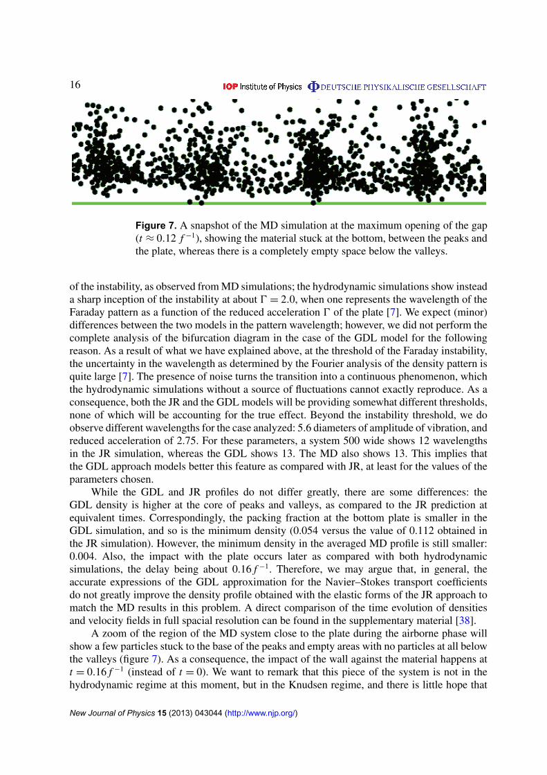
Figure 7. A snapshot of the MD simulation at the maximum opening of the gap(t ≈ 0.12 f −1), showing the material stuck at the bottom, between the peaks andthe plate, whereas there is a completely empty space below the valleys.
of the instability, as observed from MD simulations; the hydrodynamic simulations show insteada sharp inception of the instability at about 0 = 2.0, when one represents the wavelength of theFaraday pattern as a function of the reduced acceleration 0 of the plate [7]. We expect (minor)differences between the two models in the pattern wavelength; however, we did not perform thecomplete analysis of the bifurcation diagram in the case of the GDL model for the followingreason. As a result of what we have explained above, at the threshold of the Faraday instability,the uncertainty in the wavelength as determined by the Fourier analysis of the density pattern isquite large [7]. The presence of noise turns the transition into a continuous phenomenon, whichthe hydrodynamic simulations without a source of fluctuations cannot exactly reproduce. As aconsequence, both the JR and the GDL models will be providing somewhat different thresholds,none of which will be accounting for the true effect. Beyond the instability threshold, we doobserve different wavelengths for the case analyzed: 5.6 diameters of amplitude of vibration, andreduced acceleration of 2.75. For these parameters, a system 500 wide shows 12 wavelengthsin the JR simulation, whereas the GDL shows 13. The MD also shows 13. This implies thatthe GDL approach models better this feature as compared with JR, at least for the values of theparameters chosen.
While the GDL and JR profiles do not differ greatly, there are some differences: theGDL density is higher at the core of peaks and valleys, as compared to the JR prediction atequivalent times. Correspondingly, the packing fraction at the bottom plate is smaller in theGDL simulation, and so is the minimum density (0.054 versus the value of 0.112 obtained inthe JR simulation). However, the minimum density in the averaged MD profile is still smaller:0.004. Also, the impact with the plate occurs later as compared with both hydrodynamicsimulations, the delay being about 0.16 f −1. Therefore, we may argue that, in general, theaccurate expressions of the GDL approximation for the Navier–Stokes transport coefficientsdo not greatly improve the density profile obtained with the elastic forms of the JR approach tomatch the MD results in this problem. A direct comparison of the time evolution of densitiesand velocity fields in full spacial resolution can be found in the supplementary material [38].
A zoom of the region of the MD system close to the plate during the airborne phase willshow a few particles stuck to the base of the peaks and empty areas with no particles at all belowthe valleys (figure 7). As a consequence, the impact of the wall against the material happens att = 0.16 f −1 (instead of t = 0). We want to remark that this piece of the system is not in thehydrodynamic regime at this moment, but in the Knudsen regime, and there is little hope that
New Journal of Physics 15 (2013) 043044 (http://www.njp.org/)
any hydrodynamic model can reproduce this feature in full detail. However, the GDL approachto the Navier–Stokes equations improves the dynamics of the gap formed as compared withthe JR approach in the sense that the minimum density at the bottom plate is reduced. On theother hand, the density gradients are higher in the GDL theory, a feature that is not observed inthe MD profiles, which are smoother. The differences are basically due to the presence of thecoefficient µGDL (equation (19) of the GDL model), which is absent ( µJR = 0) in the elasticcase (the JR approach).
3.2. Temperature and internal energy
In figure 5, we plot the scaled internal energy, φT/(rg), where g denotes the gravityacceleration. Here we see the evolution of the shock wave traveling across the granular layer.We can observe that the energy is smaller everywhere in the GDL system, except at intermediateand large heights. Remarkably, the energy of the GDL shock wave is lower than the JR after animpact with the wall; however, the remnants persist for long at larger heights. The MD profileindicates a higher energy at the bottom after an impact (c), as compared with both GDL and JRresults, but especially with the latter. The GDL shock wave is very much damped. It also showsthat the impact with the bottom wall occurs effectively later, as pointed out when discussing thedensity profiles. In addition, the MD profile shows that the energy vanishes more quickly thanin the GDL solution. Let us examine then the temperature field.
The most striking difference between the GDL and JR solutions is the temperature field(figure 6). At large heights, the GDL temperature is one order of magnitude larger than the JR.Moreover, the GDL temperature gradient is positive at middle heights (it starts to grow), whereasthere the JR, like the MD temperature gradient, is negative once the shock wave is dissipated. Itis clear that the term µ∇n helps to sustain large temperature gradients in the system, transferringheat from the dense to the dilute regions at the top wall. This term is the genuine contribution ofthe inelastic nature of the granular gas to the transport coefficients, although we find no hint inthe obtained MD profile that the temperature gradient should be positive instead of negativewhen ascending from the dense to the dilute region. As mentioned in the introduction, thepresence of the coefficient µ in the heat flux is an exact result of the inelastic Enskog equationand the JR approximation fails in describing this new effect. In addition, the existence of thisterm in the heat flux has been already confirmed by computer simulation results [25].
However, one must recall that beyond 40 diameters in height the material gets more andmore rarefied (figure 4) and goes from densities of the order of 1% in packing fraction at 40diameters to about 0.1% at 60, as obtained from MD results. Therefore, one should find Knudsenlayers when approaching a virtual top wall—in our MD simulations there is none, making ourhydrodynamic simulations meaningless there. Note, on the other hand, that the temperature fieldT displayed in figure 6, when scaled with the mean free path as the relevant unit length, willbe proportional to the quantity φT displayed in figure 5. In the latter, one can appreciate thatthe mismatch between JR and GDL is reduced, although it still persists. Also, by comparingthe three figures (figures 4–6), we find that the growth of the temperature starts at intermediateheights, when the density is not especially small. For this reason, one can conclude that thegrowth of the temperature is a true result of the GDL approach and not a negligible product.
As the GDL temperature is higher than the JR temperature at the top, the GDL solution ismore diffusive. Figure 8 shows the vertical component of the heat flux as a function of height,where this effect is shown: note the enhanced heat transport at intermediate heights, as compared
New Journal of Physics 15 (2013) 043044 (http://www.njp.org/)
Figure 8. Vertical component of the (reduced) heat flux as a function of height(in units of σ ) at selected times over two oscillation periods, for the JR and GDLsimulations. For the time evolution of the profiles, see [38].
New Journal of Physics 15 (2013) 043044 (http://www.njp.org/)
Figure 9. The profiles of the cooling term ζnT as a function of height (inunits of σ ), at selected times over two oscillation periods, for the JR and GDLsimulations. Note the change in the vertical scale in subfigures (b) and (c). Fortime evolution of the profiles, see [38].
New Journal of Physics 15 (2013) 043044 (http://www.njp.org/)
Figure 10. The scaled kinetic energy profiles as a function of height (in unitsof σ ), at selected times over two oscillation periods for the MD, JR and GDLsystems. For time evolution of the profiles, see [38].
New Journal of Physics 15 (2013) 043044 (http://www.njp.org/)
Figure 11. Mach number for the MD system and JR and GDL theories as afunction of time, along two periods ( f −1) of oscillation of the plate. The redcurves indicate the variable height (in diameters) which corresponds to the Machnumber shown. These heights are found as the first point in vertical directionfrom the plate where the packing fraction is 0.1.
with the JR solution. Unlike the JR case, the GDL heat flux consists of two terms, one comingfrom the temperature gradient, and the other associated, through the coefficient µ, with thedensity gradient. An analysis of the data reveals that both terms have generally opposite signs.The role of the latter contribution is to transfer heat from the dense toward the dilute regions atthe top, while the former brings energy into the granulate, from the high-temperature regionsat the top. Both terms are relevant and contribute in the same order of magnitude. So, the heattransfer dynamics is quite different in the GDL and the JR approaches, not only at the top butalso at the bottom plate when the impacts occur, in such a way that it gives rise to entirelydifferent solutions for the temperature field.
In general, the GDL system is less diffusive very close to the plate and more at intermediateheights and at the top, as compared with the JR system. The viscosities and the cooling term(see figure 9) also follow this pattern. The analysis of the results allows us to conclude that inthe JR system, most of the energy is dissipated very close to the plate, whereas much less isdiffused; in the GDL, comparatively, there is less dissipation at the plate and more diffusion.
3.3. Kinetic energy and Mach number
Figure 10 shows the scaled kinetic energy profiles. An examination of the entire sequence showsthat the maximum of the kinetic energy is achieved at t = 0.38 f −1 in the GDL simulation, att = 0.42 f −1 in the JR and at t = 0.54 f −1 in the MD. The GDL peak is the highest, more thanfour times bigger than the MD and about 50% bigger than the JR. This shows that the GDLsolution for the velocity field is also quantitatively different from the JR, a consequence of theinelasticity contributing to the viscosities. Leaving aside the mismatch at the maximum, theJR and GDL solutions go close to each other, and differently from the MD profile, due to thedelayed landing of the granular layer in the MD simulation. In any case, the comparison of thekinetic energy profiles reinforces the quite unexpected result that the GDL solution is not closerto the MD, but even further away, than the JR.
New Journal of Physics 15 (2013) 043044 (http://www.njp.org/)
Since the GDL temperature is about one order of magnitude higher than JR in the diluteregion, the Mach number is also smaller. In figure 11, we can see how the differences are veryrelevant during stages (c)–(d), when the layer has achieved its maximal extension, and wherethe JR Mach number is about twice that of the GDL. This is another fact showing that the GDLsystem is more diffusive than the JR.
The MD curve for the Mach number has been produced using the averaged density andtemperature fields in equation (29) for the sound speed, supplied with the equation of state (13).
Unlike JR and GDL approximations, the second MD peak in the Mach number is higherthan the first one. Anyway, GDL predicts better the behavior of the Mach number than JR.The values of the Mach number have been computed at the heights shown by the red curves infigure 11. They correspond to the first point, going from the dense to the dilute phase, where thepacking fraction is 0.1. There we also find discrepancies when comparing the MD results withthose of JR and GDL simulations. This is a consequence of the discrepancies in the density fielddiscussed above.
4. Conclusions
In this paper, we have compared the predictions of the Navier–Stokes hydrodynamic equationsof 2D granular gases with MD simulations in a highly nonlinear, far-from-equilibrium problemsuch as the periodic impact of a horizontal piston which gives rise to the characteristic patternformation of the Faraday instability. Given that the corresponding Navier–Stokes transportcoefficients are not exactly known, two different approaches to them have been considered:the JR and GDL approximations. While the first approach applies to nearly elastic particles(in fact, their forms for the transport coefficients are the same as the elastic ones), the latterapproximation is much more accurate for granular gases (as verified, for instance, in [23] bycomparing the GDL theory with computer simulations at quite extreme values of dissipation)since it incorporates the effect of inelasticity on the transport coefficients. In particular, whilethe JR theory neglects the term −µ E∇n in the heat flux, the new transport coefficient µ is clearlydifferent from zero in the GDL theory (see the fourth panel of figure 1). After comparing bothapproaches with coarse-grained MD results, we can conclude on the following relevant aspects.
First, we conclude that the granular Navier–Stokes hydrodynamics with the properGDL forms for the transport coefficients η, γ , κ and µ is not capable of reducing thediscrepancy between discrete particle simulations and hydrodynamic simulations of moderatelydense, inelastic gases. This quantitative disagreement can be due to the fact that while theNavier–Stokes constitutive equations (4) and (5) for the pressure tensor and the heat flux,respectively, apply to first-order in the spatial gradients, the problem analyzed here might beoutside the strict validity of the Navier–Stokes approximation as the comparison with MDsimulations shows. Surprisingly, the discrepancies between theory and simulations decrease ifone considers the elastic forms of the transport coefficients. We think that there are no physicalreasons behind this improvement. A similar conclusion has been found in the simple shear flowproblem for dilute gases since the non-Newtonian shear viscosity ηs(α) to be plugged into theNavier–Stokes hydrodynamic equations is better modeled by the elastic shear viscosity than itscorresponding inelastic version ηGDL(α) (see figure 1 of [32], where while ηs decreases withdecreasing α, the opposite happens for ηGDL).
Apart from the different α dependence of η, γ and κ , the main difference between the JRand GDL approaches lies in the presence of the coefficient µ in the heat flux. This new transport
New Journal of Physics 15 (2013) 043044 (http://www.njp.org/)
coefficient, characteristic of inelastic gases and thus vanishing in the JR theory, constitutesa significant contribution to an enhanced heat transfer mechanism which leads to a high-temperature solution in the dilute region, which is not supported by the particle simulations.Even in the dilute region at the top of the system (figure 1), where shock waves should becompletely damped, the GDL model produces an unrealistic energy excess. There, at densitiesof the order of 0.001 in packing fraction, the coefficient µ is very different from zero.
Thus, we can conclude that the transport coefficient µ is clearly overestimated by theNavier–Stokes approximation and, consequently, the influence of the diffusion term −µ E∇non the heat flux is larger than that observed in the simulations. As mentioned before, thesediscrepancies do not imply that the GDL approach is deficient in any respect. Rather differently,they show the limits of the Navier–Stokes description applied to certain regimes of complexgranular flow.
As a matter of fact, in the theory of granular gases, it is well accepted that in certain casesthe Navier–Stokes description is insufficient. It was clearly evidenced at the mathematical level,e.g. in [42], that Burnett-order terms are important for the kinetics of granular gases. Theseterms in the constitutive relations are of second order in the gradients and therefore beyond theNavier–Stokes level of description. In [42], it was shown that these terms are even necessaryfor a consistent description due to the lack of scale separation in granular gases. The presenceof large gradients is quite usual in granular flow, where physical variables may change severalorders of magnitude within a distance of a few grains, due to inelastic interactions. That typicallymanifests in strong shock waves propagating into the system from the boundaries, where theenergy source is located. In this way, granular flow is very often supersonic or even hypersonic,and in this regime of extreme gradients the Navier–Stokes description may prove inadequate.
The inclusion of higher-order terms (beyond the Navier–Stokes domain) in the constitutiveequations for the momentum and heat fluxes might prove to be a better approximation toproblems such as this one, where the first order in the gradients expansion seems insufficient.However, the determination of these nonlinear contributions to the fluxes becomes a very hardtask if one starts from the revised Enskog equation. In these cases it is useful to consider kineticmodels with the same qualitative features as the Enskog equation but with a mathematicallysimpler structure [43]. The use of these models allows to derive explicit forms for generalizedconstitutive equations in complex states driven far from equilibrium, such as the simple shearflow state [44].
In spite of the discrepancies found here, the Navier–Stokes approximation with theGDL forms for the transport coefficients is still appropriate and accurate for a wide class offlows. Some examples include applications of the Navier–Stokes hydrodynamics to symmetrybreaking and density/temperature profiles in vibrated gases [26, 27], binary mixtures [45] andsupersonic flow past a wedge in real experiments [4, 46, 47]. Another group refers to spatialperturbations of the homogeneous cooling state for an isolated system where the MD results ofthe critical length for the onset of vortices and clusters [48, 49] are successfully compared withthe predictions from linear stability analysis [50] performed on the basis of the GDL transportcoefficients.
In summary, the Navier–Stokes theory has shown limitations when exploring the highlynonlinear problem of granular Faraday instability. In particular, the presence of rarefied regionswhere strong transient shock wave fronts propagate seems to justify the inclusion of higher-order gradients in the transport equations, going beyond the Navier–Stokes approximation [42].In spite of that, both GDL and JR models work quite well, although here the main discrepancy
New Journal of Physics 15 (2013) 043044 (http://www.njp.org/)
is attributed to the term in the heat flux coupled to the density gradient, which is the missingcontribution in the JR approach that the inelastic theory comes to fix. More work has to bedone in this respect to clarify the conditions under which the Navier–Stokes approximation failsto describe appropriately the granular heat transport. Finally, as a complementary route to theNavier–Stokes approximation, one could numerically solve the Enskog equation via the directsimulation Monte Carlo method [51, 52]. Presumably, the numerical solution would give betterquantitative agreement with MD simulations than the Navier–Stokes results reported here. Thisis quite an interesting problem to be addressed in the future for the Faraday and other differentproblems such as the simple shear flow or homogeneous states.
Acknowledgments
LA and JAC were partially supported by the project MTM2011-27739-C04-02 DGI (Spain) and2009-SGR-345 from AGAUR-Generalitat de Catalunya. LA, JAC and CS acknowledge supportfrom the project Ingenio Mathematica FUT-C4-0175. CS and VG acknowledge funding fromprojects DPI2010-17212 (CS) and FIS2010-16587 (VG) of the Spanish Ministry of Science andInnovation. The latter project (FIS2010-16587) is partially financed by FEDER funds and by theJunta de Extremadura (Spain) through grant number GR10158. LA and TP were supported byDeutsche Forschungsgemeinschaft through the Cluster of Excellence Engineering of AdvancedMaterials. JAC acknowledges support from the Royal Society through a Wolfson ResearchMerit Award. This work was supported by the Engineering and Physical Sciences ResearchCouncil under grant number EP/K008404/1.
References
[1] Jenkins J and Richman M W 1985 Arch. Ration. Mech. Anal. 87 355[2] Jenkins J and Richman M W 1985 Phys. Fluids 28 3485[3] Bizon C, Shattuck M D, Swift J B and Swinney H L 1999 Phys. Rev. E 60 4340[4] Rericha E C, Bizon C, Shattuck M D and Swinney H L 2001 Phys. Rev. Lett. 88 014302[5] Bougie J, Moon S J, Swift J B and Swinney H L 2002 Phys. Rev. E 66 051301[6] Bougie J, Kreft J, Swift J B and Swinney H L 2005 Phys. Rev. E 71 021301[7] Carrillo J A, Poschel T and Saluena C 2008 J. Fluid Mech. 597 119[8] Bougie J 2010 Phys. Rev. E 81 032301[9] Bougie J and Duckert K 2011 Phys. Rev. E 83 011303
[10] Melo F, Umbanhowar P and Swinney H L 1994 Phys. Rev. Lett. 72 172[11] Melo F, Umbanhowar P B and Swinney H L 1995 Phys. Rev. Lett. 75 3838[12] Hill S A and Mazenko G F 2003 Phys. Rev. E 67 061302[13] Brilliantov N V, Saluena C, Schwager T and Poschel T 2004 Phys. Rev. Lett. 93 134301[14] Meerson B, Poschel T and Bromberg Y 2003 Phys. Rev. Lett. 91 024301[15] Meerson B, Poschel T, Sasorov P V and Schwager T 2004 Phys. Rev. E 69 021302[16] Eshuis P, van der Meer D, Alam M, van Gerner H J, van der Weele K and Lohse D 2010 Phys. Rev. Lett.
104 038001[17] Faraday M 1831 Phil. Trans. R. Soc. 121 299[18] Garzo V and Dufty J W 1999 Phys. Rev. E 59 5895[19] Lutsko J F 2005 Phys. Rev. E 72 021306[20] Chapman S and Cowling T G 1970 The Mathematical Theory of Nonuniform Gases (London: Cambridge
University Press)
New Journal of Physics 15 (2013) 043044 (http://www.njp.org/)
[21] Brey J J and Ruiz-Montero M J 2004 Phys. Rev. E 70 051301[22] Brey J J, Ruiz-Montero M J, Maynar P and Garcıa de Soria I 2005 J. Phys.: Condens. Matter 17 S2489[23] Garzo V, Santos A and Montanero J M 2007 Physica A 376 94[24] Shu C W 1998 Advanced Numerical Approximation of Nonlinear Hyperbolic equations (Lecture Notes in
Mathematics vol 1697) ed C Cockburn, B Johnson, C W Shu and E Tadmor (Berlin: Springer) p 325[25] Soto R, Mareschal M and Risso D 1999 Phys. Rev. Lett. 83 5003[26] Brey J J, Ruiz Montero M J and Moreno F 2001 Phys. Rev. E 63 061305[27] Brey J J, Ruiz Montero M J, Moreno F and Garcıa Rojo R 2002 Phys. Rev. E 65 061302[28] Goldshtein A and Shapiro M 1995 J. Fluid Mech. 282 75[29] Brey J J, Dufty J W and Santos A 1997 J. Stat. Phys. 87 1051[30] Brilliantov N and Poschel T 2004 Kinetic Theory of Granular Gases (Oxford: Oxford University Press)[31] Goldhirsch I 2003 Annu. Rev. Fluid Mech. 35 267[32] Santos A, Garzo V and Dufty J W 2004 Phys. Rev. E 69 061303[33] Grad H 1949 Commun. Pure Appl. Math. 2 331[34] Gass D M 1970 J. Chem. Phys. 54 1898[35] Torquato S 1995 Phys. Rev. E 51 3170[36] Garzo V 2012 arXiv:1204.5114[37] Jiang G and Shu C W 1996 J. Comput. Phys. 126 202[38] Almazan L, Carrillo J A, Garzo V, Saluena C and Poschel T 2012 Supplementary Online Material
http://msssrv01.mss.uni-erlangen.de/lidia/[39] van Noije T P C, Ernst M H, Brito R and Orza J A G 1997 Phys. Rev. Lett 79 411[40] Brey J, Maynar P and Garcia de Soria M I 2009 Phys. Rev. E 79 051305[41] Costantini G and Puglisi A 2010 Phys. Rev. E 82 011305[42] Goldhirsch I 2008 Powder Technol. 182 130[43] Brey J J, Dufty J W and Santos A 1999 J. Stat. Phys. 97 281[44] Montanero J M, Garzo V, Santos A and Brey J J 1999 J. Fluid Mech. 389 391[45] Dahl S R, Hrenya C M, Garzo V and Dufty J W 2002 Phys. Rev. E 66 041301[46] Yang X, Huan C, Candela D, Mair R W and Walsworth R L 2002 Phys. Rev. Lett. 88 044301[47] Huan C, Yang X, Candela D, Mair R W and Walsworth R L 2004 Phys. Rev. E 69 041302[48] Mitrano P P, Dahl S R, Cromer D J, Pacella M S and Hrenya C M 2011 Phys. Fluids 23 093303[49] Mitrano P P, Garzo V, Hilger A H, Ewasko C J and Hrenya C M 2012 Phys. Rev. E 85 041303[50] Garzo V 2005 Phys. Rev. E 72 021106[51] Bird G A 1994 Molecular Gas Dynamics and the Direct Simulation of Gas Flows (Oxford: Clarendon)[52] Montanero J M and Santos A 1996 Phys. Rev. E 54 438
New Journal of Physics 15 (2013) 043044 (http://www.njp.org/)


![arXiv · arXiv:1702.07045v1 [math.AP] 22 Feb 2017 WEIGHTED Lq-ESTIMATES FOR STATIONARY STOKES SYSTEM WITH PARTIALLY BMO COEFFICIENTS HONGJIE DONG …](https://static.documents.pub/doc/80x56/613b08e2f8f21c0c8268c6b1/arxiv-arxiv170207045v1-mathap-22-feb-2017-weighted-lq-estimates-for-stationary.jpg)


