A NUMERICAL STUDY ON THE WEAK GALERKIN METHOD FORTHE HELMHOLTZ EQUATION WITH LARGE WAVE NUMBERS

LIN MU∗, JUNPING WANG† , XIU YE‡ , AND SHAN ZHAO§

Abstract. Weak Galerkin (WG) refers to general finite element methods for partial differentialequations in which differential operators are approximated by weak forms through the usual inte-gration by parts. In particular, WG methods allow the use of discontinuous finite element functionsin the algorithm design. One of such examples was recently introduced in [54] for solving secondorder elliptic problems. The goal of this paper is to apply the WG method of [54] to the Helmholtzequation with high wave numbers. Several test scenarios are designed for a numerical investigationon the accuracy, convergence, and robustness of the WG method in both inhomogeneous and ho-mogeneous media over convex and non-convex domains. Our numerical experiments indicate thatweak Galerkin is a finite element technique that is easy to implement, and provides very accurateand robust numerical solutions for the Helmholtz problem with high wave numbers.

Key words. Galerkin finite element methods, discrete gradient, the Helmholtz equation, weakGalerkin

AMS subject classifications. Primary, 65N15, 65N30, 76D07; Secondary, 35B45, 35J50

1. Introduction. In this paper, we explore the use of a weak Galerkin (WG)finite element method for solving the nonhomogeneous Helmholtz equation with highwave numbers

(1.1) −∇ · (d∇u)− k2u = f,

where k is the wave number, f represents a harmonic source, and d = d(x, y) is a spa-tial function describing the dielectric properties of the medium. The Helmholtz equa-tion (1.1) governs many macroscopic wave phenomena in the frequency domain in-cluding wave propagation, guiding, radiation and scattering, where the time-harmonicbehavior can be assumed. The numerical solution to the Helmholtz equation plays avital role in a wide range of applications in electromagnetics, optics, and acoustics,such as antenna analysis and synthesis, radar cross section calculation, simulation ofground or surface penetrating radar, design of optoelectronic devices, acoustic noisecontrol, and seismic wave propagation. However, it remains a challenge to designrobust and efficient numerical algorithms for the Helmholtz equation, especially whenhigh wave numbers or highly oscillatory solutions are involved [58].

Physically, the Helmholtz problem is usually defined on an unbounded exteriordomain with the so-called Sommerfeld radiation condition holding at infinity [38, 53]

(1.2)∂u

∂r− iku = o

(r

1−m2

), as r →∞, m = 2, 3.

∗Department of Applied Science, University of Arkansas at Little Rock, Little Rock, AR 72204(lxmu@ualr.edu).†Division of Mathematical Sciences, National Science Foundation, Arlington, VA 22230 (jwang@

nsf.gov). The research of Wang was supported by the NSF IR/D program, while working at theFoundation. However, any opinion, finding, and conclusions or recommendations expressed in thismaterial are those of the author and do not necessarily reflect the views of the National ScienceFoundation.‡Department of Mathematics and Statistics, University of Arkansas at Little Rock, Little Rock,

AR 72204 (xxye@ualr.edu). This research of Ye was supported in part by National Science Founda-tion Grant DMS-1115097.§Department of Mathematics, University of Alabama, Tuscaloosa, AL 35487

(szhao@bama.ua.edu). The research of Zhao was supported in part by National Science FoundationGrant DMS-1016579.

1

arX

iv:1

111.

0671

v1 [

mat

h.N

A]

2 N

ov 2

011

2

where i =√−1 is the imaginary unit and r is the radial direction. Here we have

assumed that d = 1 in far field. In computational electromagnetics, the exteriordomain problems are often solved numerically by introducing a bounded domain Ωwith an artificial boundary ∂Ω and imposing certain boundary conditions on ∂Ω sothat nonphysical reflections from the boundary can be eliminated or minimized. Forthe Helmholtz exterior problems, the non-reflecting condition is commonly chosenas a Dirichlet-to-Neumann (DtN) mapping, which relates the wave solution to itsderivatives on ∂Ω [38, 53]

(1.3) d∇u · n− T (u) = g, on ∂Ω,

where n denotes the outward normal direction of ∂Ω, T is a DtN integral operator, andg is a given data function. For sufficiently large Ω, the nonlocal boundary condition(1.3) can be approximated by a Robin boundary condition [38, 53]

(1.4) d∇u · n− iku = g, on ∂Ω,

which is essentially a first order absorbing boundary condition.In the present paper, we consider the following prototype Helmholtz problem

−∇ · (d∇u)− k2u = f in Ω,(1.5)

d∇u · n− iku = g on ∂Ω.(1.6)

Finite element methods for such Helmholtz problems can be classified as two cate-gories. The first category consists of methods that use continuous functions to approx-imate the solution u and the other refers to methods with discontinuous approximationfunctions.

Continuous Galerkin (CG) finite element methods employ continuous piecewisepolynomials to approximate the true solution of (1.5)-(1.6) and lead to a simple for-mulation: find uh ∈ Vh ⊂ H1(Ω) satisfying

(1.7) (d∇uh,∇vh)− k2(uh, vh) + ik(uh, vh)∂Ω = (f, vh) + (g, vh)∂Ω

for all vh ∈ Vh, where Vh is an properly defined finite element space consisting ofcontinuous piecewise polynomials.

Discontinuous Galerkin (DG) finite element methods for the Helmholtz equationwith d = 1 (e.g. [33]) seek uh ∈ Vh ⊂ L2(Ω) satisfying∑T

(∇uh,∇vh)T−∑e

((∇uh, [vh])e + σ(∇vh, [uh])e)− k2(uh, vh)

+ik(uh, vh)∂Ω + i(∑e

α1h−1e ([uh], [vh])e +

∑e

α2he([∂uh∂n

], [∂vh∂n

])e

+∑e

α3h−1e ([

∂uh∂t

], [∂vh∂t

])e) = (f, vh) + (g, vh)∂Ω,(1.8)

for all vh ∈ Vh, where αi, i=1,2,3 are penalty parameters and Vh is a space of discon-tinuous piecewise polynomials.

The continuous Galerkin finite element formulation (1.7) is natural and easy toimplement. However, the errors of continuous Galerkin finite element solutions de-teriorate rapidly when k becomes large. On the other hand, the formulation of DG

3

methods (1.8) is complex, and the stability and accuracy of DG methods heavily de-pend on the selection of penalty parameters (a good determination for the parametervalues has been an issue for DG methods).

The objective of the present paper is to introduce a weak Galerkin (WG) finiteelement method for solving the Helmholtz problem with high wave numbers and toinvestigate the robustness and effectiveness of such WG method through many care-fully designed numerical experiments. The weak Galerkin finite element formulationwas first developed in [54] for solving the second order elliptic equations. Throughrigorous error analysis, optimal order of convergence of the WG solution in both dis-crete H1 norm and L2 norm is established under minimum regularity assumptions in[54]. Nevertheless, no experimental results have been reported in [54].

Generally speaking, like the DG method, the WG finite element method allows oneto use discontinuous functions in the finite element procedure. The main idea behindweak Galerkin methods lies in the approximation of differential operators by weakforms for discontinuous finite element functions defined on a partition of the domain.For example, for the gradient operator, one may introduce a weak gradient operator∇d over discontinuous functions vh = v0, vb, where v0 is defined in the interior ofthe element and vb is defined on the boundary of the element. The weak gradientoperator will then be employed to form a weak Galerkin finite element formulationfor (1.5)-(1.6): find uh ∈ Vh such that for all vh ∈ Vh we have

(1.9) (d∇duh,∇dvh)− k2(u0, v0) + ik(ub, vb)∂Ω = (f, v0) + (g, vb)∂Ω.

The discrete gradient ∇dv in (1.9) is a variable locally calculated on each element.The weak Galerkin methods have many nice features. First, the formulation of WGmethod is simple, easy to implement, and involves no penalty parameters for usersto select. The weak Galerkin is equipped with elements of polynomials of any degreek ≥ 0. Secondly, the weak Galerkin method conserves mass with a well definednumerical flux. In some sense, weak Galerkin finite element methods enjoy both thesimplicity of CG method and the flexibility of DG method.

In the present numerical investigation, we are particularly interested in the perfor-mance of the WG method for solving the Helmholtz equation with high wave numbers.In general, the numerical performance of any finite element solution to the Helmholtzequation depends significantly on the wave number k. When k is very large – repre-senting a highly oscillatory wave, the mesh size h has to be sufficiently small for thescheme to resolve the oscillations. To keep a fixed grid resolution, a natural rule is tochoose kh to be a constant in the mesh refinement, as the wave number k increases[41, 12]. However, it is known [41, 42, 8, 9] that, even under such a mesh refinement,the errors of continuous Galerkin finite element solutions deteriorate rapidly when kbecomes larger. This non-robust behavior with respect to k is known as the “pollutioneffect” [41, 42, 8, 9]. Usually, under the small magnitude assumption of kh, the rela-tive error of a pth order finite element solution in the H1-semi-norm consists of twoparts [41, 42], i.e., an error term of the best approximation behavior like O(kphp) anda pollution error term behavior like O(k2p+1h2p). The error of best approximationis essentially due to the interpolation error on a discretized grid and is of boundedmagnitude if kh = constant. Nevertheless, the pollution error term dominates whenk is large and is responsible for the non-robustness behavior in the finite elementsolutions to the Helmholtz equation.

To the end of eliminating or substantially reducing the pollution errors, variousnumerical approaches have been developed in the literature for solving the Helmholtz

4

equation. For the continuous and least-squares finite element methods, a popularstrategy [8, 9, 45, 10, 46] to reduce the pollution error is to include some analyticalknowledge of the problem, such as characteristics of asymptotic or exact solution, inthe finite element space. The resulting local basis functions of non-polynomial shapeyield improved performance [8, 9, 45, 10, 46]. Similarly, analytical information isincorporated in the basis functions of the boundary element methods to address thehigh frequency problems [36, 44, 23]. Based on the geometrical optics and geometricaltheory of diffraction, asymptotic solutions of the Helmholtz equation that representimportant wave propagation directions are coupled with high frequency oscillations tobuilt boundary element approximation spaces. Consequently, the number of degreesof freedom of such boundary element methods virtually does not depend on the wavenumber k for the Helmholtz equation [36, 44, 23]. In [22], plane wave solutionstraveling in a large number of directions have also been employed as basis functions inthe ultra weak variational formulation (UWVF) [21]. This allows the use of a coarsemesh when resolving high oscillatory wave solutions. The UWVF method can beregarded as an upwinding DG discretization for a first order system obtained throughthe introduction of an adjoint field. Based on such a viewpoint, error estimates ofthe UWVF on the entire domain have been recently presented in [19]. Multiple planewave basis functions are also employed in a DG method using both low order elements[31] and high order elements [32]. The weak continuity of the solution at the elementboundaries is enforced by introducing a Lagrange multiplier. Being more robust thanclassical variational approaches, this DG method can resolve high frequency shortwave problems very well with a ratio of up to three wavelengths per element [31, 32].

Besides changing basis functions, there are other improvements that can be madein the DG framework to reduce the pollution error. By using piecewise linear polyno-mials as the basis functions, stable interior penalty DG methods have been developedin [33] through penalizing not only the jumps of the function values, but also thejumps of the normal and tangential derivatives across the element edges. Robustresults against pollution effect can be achieved through a careful selection of penaltyparameters [33]. Also targeting on enhancing stability, DG methods can be estab-lished by formulating the wave equation as a first-order system [6, 25]. The classicaltechniques, such as the enforcement of weak continuity via fluxes form, can be used insuch DG solutions to the Helmholtz equation. The dispersive and dissipative behaviorof selected DG schemes for both second order Helmholtz equation and the correspond-ing first order system have been examined in [2]. Hybridizable DG method is anotherefficient finite element method for the Helmholtz equation [29, 30]. By introducingnew degree of freedoms on the boundary of elements, parametrization is conductedelement by element so that the final linear system consists of unknowns only from theskeleton of the mesh. This greatly reduces the size of linear systems compared to thestandard DG scheme. The error analysis [37] shows that the condition number of thecondensed matrix of the hybridizable DG methods [29, 30] could be independent ofthe wave number.

The pollution effect can also be alleviated by controlling the numerical dispersion,i.e., the phase difference between the numerical and exact waves. This is because thepollution error is known to be directly related to the dispersion error [40, 1], whilethe best approximation error is non-dispersive. Thus, the reduction of the dispersiveerror is equivalent to the reduction of the pollution error. Consequently, high ordermethods, such as local spectral method [12], spectral Galerkin methods [52, 53], andspectral element methods [39, 3] are less vulnerable to the pollution effect, because

5

they produce negligible dispersive errors.The rest of this paper is organized as follows. In Section 2, we will introduce

a weak Galerkin finite element method for the Helmholtz equation by following theidea presented in [54]. In Section 3, we will present some error estimates for theWG method for the Helmholtz equation. Finally in Section 4, we shall present somenumerical results obtained from the weak Galerkin method with various orders.

2. A Weak Galerkin Finite Element Method. Let Th be a partition of thedomain Ω with mesh size h. Assume that the partition Th is shape regular so that theroutine inverse inequality in the finite element analysis holds true (see [26]). Define(v, w)K =

∫Kvwdx and (v, w)∂K =

∫∂K

vwds.For each triangle T ∈ Th, let T 0 and ∂T denote the interior and boundary of

T respectively. Denote by Pj(T0) the set of polynomials in T 0 with degree no more

than j, and P`(∂T ) the set of polynomials on each segment (edge or face) of ∂T withdegree no more than `. We emphasize that functions of P`(∂T ) are defined on eachedge/face and there is no continuity required across different edges/faces. Define aglobal function v = v0, vb where v0 and vb represent the values of v on T 0 and∂T respectively for each T ∈ Th. Now we are ready to define a weak Galerkin finiteelement space as follows

(2.1) Vh =v = v0, vb : v0, vb|T ∈ Pj(T 0)× P`(∂T ),∀T ∈ Th

.

For each v = v0, vb ∈ Vh, we define the discrete gradient of v on each element T bythe following equation:

(2.2)

∫T

∇dv · qdT = −∫T

v0∇ · qdT +

∫∂T

vbq · nds, ∀q ∈ Vr(T ),

where Vr(T ) is a subspace of the set of vector-valued polynomials of degree no morethan r on T .

For the purpose of easy demonstration, we consider a special 2-D weak Galerkinelement of Vh and Vr(T ) with j = ` = k ≥ 0 in (2.1) and Vr(T ) = RTk(T ). More weakGalerkin elements can be found in [54]. Here RTk(T ) is the usual Raviart-Thomaselement [47] of order k which has the form

RTk(T ) = Pk(T )2 + Pk(T )x,

where Pk(T ) is the set of homogeneous polynomials of degree k and x = (x1, x2).

Weak Galerkin Algorithm 1. A numerical approximation for (1.5)-(1.6)can be obtained by seeking uh = u0, ub ∈ Vh such that for all vh = v0, vb ∈ Vh

(2.3) (d∇duh,∇dvh)− k2(u0, v0) + ik(ub, vb)∂Ω = (f, v0) + (g, vb)∂Ω.

In the following, we will use the lowest order weak Galerkin element (k=0) asan example to demonstrate how one might implement weak Galerkin finite elementmethod for solving the Helmholtz problem (1.5)-(1.6). Let N(T ) and N(e) denote thenumber of triangles and the number of edges associated with triangulation Th. LetEh denote the union of the boundaries of the triangles T of Th. Let φi be a functionwhich takes value one in the interior of triangle Ti and zero everywhere else. Let ψjbe a function that takes value one on edge ej and zero everywhere else. The weakGalerkin finite element space Vh with k = 0 has the form

Vh = spanφ1, · · · , φN(T ), ψ1, · · · , ψN(e).

6

The methodology of implementing WG is the same as that for continuous Galerkinfinite element method except that the standard gradient operator ∇ must be replacedby the discrete gradient operator ∇d. The discrete gradient operator is an exten-sion of the standard gradient operator for smooth functions to non-smooth functions.Therefore, the key step of implementing weak Galerkin method is to compute a localvariable ∇dv for v = v0, vb ∈ Vh element by element. For the case k = 0, we have∇dv ∈ RT0(T ) on each element T ∈ Th where

RT0(T ) =

(a+ cxb+ cy

)= spanθ1, θ1, θ3.

For example, we can choose θi as follows

θ1 =

(10

), θ2 =

(01

), θ3 =

(xy

).

Thus on each element T ∈ Th, ∇dv =∑3j=1 cjθj . Using the definition of discrete

gradient (2.2), we find cj by solving the following linear system: (θ1, θ1)T (θ2, θ1)T (θ3, θ1)T(θ1, θ2)T (θ2, θ2)T (θ3, θ2)T(θ1, θ3)T (θ2, θ3)T (θ3, θ3)T

c1c2c3

=

−(v0,∇ · θ1)T + (vb, θ1 · n)∂T−(v0,∇ · θ2)T + (vb, θ2 · n)∂T−(v0,∇ · θ3)T + (vb, θ3 · n)∂T

.

The inverse of the above coefficient matrix can be obtained explicitly or numericallythrough a local matrix solver. Once ∇dφi and ∇dψj are computed, the rest of stepsare the same as those for the classical finite element method.

3. Error Estimates. Denote by Qhu = Q0u, Qbu the L2 projection ontoPj(T

0)× Pj(∂T ). In other words, on each element T , the function Q0u is defined asthe L2 projection of u in Pj(T ) and on ∂T , Qbu is the L2 projection in Pj(∂T ).

Consider the following Helmholtz problem:

−∇ · (d∇u)− k2u = f in Ω,(3.1)

u = g on ∂Ω.(3.2)

For weak Galerkin finite element space Vh defined in (2.1), we define V 0h a subspace

of Vh with vanishing boundary values on ∂Ω; i.e.,

V 0h := v = v0, vb ∈ Vh, vb|∂T∩∂Ω = 0, ∀T ∈ Th .

The weak Galerkin finite element method for the Helmholtz problem (3.1)-(3.2) isstated as follows.

Weak Galerkin Algorithm 2. A numerical approximation for (3.1) and (3.2)can be obtained by seeking uh = u0, ub ∈ Vh satisfying ub = Qbg on ∂Ω and thefollowing equation:

(3.3) (d∇duh, ∇dv)− k2(u0, v0) = (f, v0), ∀ v = v0, vb ∈ V 0h ,

For a sufficiently small mesh size h, the following error estimate holds true. Aproof of this error estimate can be found in [54].

Theorem 3.1. Let u ∈ H1(Ω) be the solution (3.1) and (3.2), and uh be a weakGalerkin approximation of u arising from (3.3). Assume that the exact solution u is

7

sufficiently smooth such that u ∈ Hm+1(Ω) with 0 ≤ m ≤ k + 1. Then, there exists aconstant C such that

‖∇d(uh −Qhu)‖ ≤ C(hm‖u‖m+1 + h1+s‖f −Q0f‖)(3.4)

‖uh −Qhu‖ ≤ C(hm+s‖u‖m+1 + h1+s‖f −Q0f‖),(3.5)

provided that the dual problem of (3.1)-(3.2) has the Hm+s(Ω) regularity with s ∈(0, 1].

4. Numerical Experiments. In this section, we examine the WG methodby testing its accuracy, convergence, and robustness for solving two dimensionalHelmholtz equations. The pollution effect due to large wave numbers will be par-ticularly investigated and tested numerically. For convergence tests, both piecewiseconstant and piecewise linear finite elements will be considered. To demonstrate WG’srobustness, the Helmholtz equation in both homogeneous and inhomogeneous mediawill be solved on convex and non-convex computational domains. For simplicity, astructured triangular mesh is employed in all cases. The mesh generation and allcomputations are conducted in the MATLAB environment.

Two types of relative errors are measured in our numerical experiments. The firstone is the relative L2 error and the second is the relative H1 error. The relative L2

error is defined by

‖uh −Qhu‖‖Qhu‖

,

where uh is the WG approximation to the solution u, and Qhu = Q0u,Qbu is theL2 projection onto Pj(T

0)×Pj(∂T ). In other words, on each element T , the functionQ0u is defined as the L2 projection of u in Pj(T ) and on ∂T , Qbu is the L2 projectionin Pj(∂T ). The relative H1 error is defined in terms of the discrete gradient

‖∇d(uh −Qhu)‖‖∇dQhu‖

.

However, in the present study, the H1-semi-norm will be calculated as

|||uh −Qhu|||2 = h−1e 〈u0 − ub − (Q0u−Qbu), u0 − ub − (Q0u−Qbu)〉e

for the lowest order finite element (i.e., piecewise constants). For piecewise linearelements, we use the original definition of ∇d to compute the H1-semi-norm ‖∇d(uh−Qhu)‖.

4.1. A convex Helmholtz problem. We first consider a homogeneous Helmholtzequation defined on a convex hexagon domain, which has been studied in [33]. Thedomain Ω is the unit regular hexagon domain centered at the origin (0, 0), see Fig.

4.1 (left). Here we set d = 1 and f = sin(kr)/r in (1.5), where r =√x2 + y2. The

boundary data g in the Robin boundary condition (1.6) is chosen so that the exactsolution is given by

u =cos(kr)

k− cos k + i sin k

k(J0(k) + iJ1(k))J0(kr)(4.1)

where Jξ(z) are Bessel functions of the first kind. Let Th denote the regular triangu-lation that consists of 6N2 triangles of size h = 1/N , as shown in Fig. 4.1 (left) forT 1

8.

8

−1 −0.5 0 0.5 1−1

−0.5

0

0.5

1

−1 −0.5 0 0.5 1−1

−0.5

0

0.5

1

Fig. 4.1. Geometry of testing domains and sample meshes. Left: a convex hexagon domain;Right: a non-convex imperfect circular domain.

Table 4.1Convergence of piecewise constant WG for the Helmholtz equation on a convex domain with

wave number k = 1.

relative H1 relative L2

h error order error order5.00e-01 2.49e-02 4.17e-032.50e-01 1.11e-02 1.16 1.05e-03 1.991.25e-01 5.38e-03 1.05 2.63e-04 2.006.25e-02 2.67e-03 1.01 6.58e-05 2.003.13e-02 1.33e-03 1.00 1.64e-05 2.001.56e-02 6.65e-04 1.00 4.11e-06 2.00

Table 4.2Convergence of piecewise linear WG for the Helmholtz equation on a convex domain with wave

number k = 5.

relative H1 relative L2

h error order error order2.50e-01 9.48e-03 2.58e-041.25e-01 2.31e-03 2.04 3.46e-05 2.906.25e-02 5.74e-04 2.01 4.47e-06 2.953.13e-02 1.43e-04 2.00 5.64e-07 2.991.56e-02 3.58e-05 2.00 7.06e-08 3.007.81e-03 8.96e-06 2.00 8.79e-09 3.01

Table 4.1 illustrates the performance of the WG method with piecewise constantelements for the Helmholtz equation with wave number k = 1. Uniform triangularpartitions were used in the computation through successive mesh refinements. Therelative errors in L2 norm and H1 semi-norm can be seen in Table 4.1. The Tablealso includes numerical estimates for the rate of convergence in each metric. It canbe seen that the order of convergence in the relative H1 semi-norm and relative L2

norm are, respectively, one and two for piecewise constant elements.

9

−1 −0.5 0 0.5 1−1

−0.5

0

0.5

1

−0.3

−0.2

−0.1

0

0.1

0.2

0.3

0.4

0.5

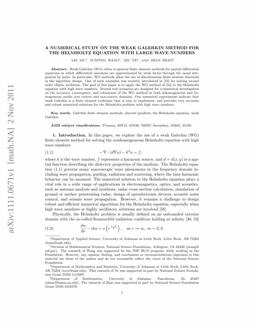
Fig. 4.2. WG solutions for the non-convex Helmholtz problem with k = 4 and ξ = 1. Left:Mesh level 1; Right: Mesh level 6.

High order of convergence can be achieved by using corresponding high orderfinite elements in the present WG framework. To demonstrate this phenomena, weconsider the same Helmholtz problem with a slightly larger wave number k = 5. TheWG with piecewise linear functions was employed in the numerical approximation.The computational results are reported in Table 4.2. It is clear that the numericalexperiment validates the theoretical estimates. More precisely, the rates of conver-gence in the relative H1 semi-norm and relative L2 norm are given by two and three,respectively.

4.2. A non-convex Helmholtz problem. We next explore the use of the WGmethod for solving a Helmholtz problem defined on a non-convex domain, see Fig.4.1 (right). The medium is still assumed to be homogeneous, i.e., d = 1 in (1.5). Weare particularly interested in the performance of the WG method for dealing with thepossible field singularity at the origin. For simplicity, only the piecewise constant RT0

elements are tested for the present problem. Following [37], we take f = 0 in (1.5)and the boundary condition is simply taken as a Dirichlet one: u = g on ∂Ω. Here gis prescribed according to the exact solution [37]

(4.2) u = Jξ(k√x2 + y2) cos(ξ arctan(y/x)).

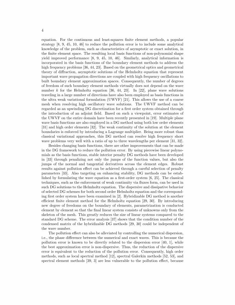
In the present study, the wave number was chosen as k = 4 and three valuesfor the parameter ξ are considered; i.e., ξ = 1, ξ = 3/2 and ξ = 2/3. The sametriangular mesh is used in the WG method for all three cases. In particular, an initialmesh is first generated by using MATLAB with default settings, see Fig. 4.1 (right).Next, the mesh is refined uniformly for five times. The WG solutions on mesh level1 and mesh level 6 are shown in Fig. 4.2, Fig. 4.3, and Fig. 4.4, respectively, forξ = 1, ξ = 3/2, and ξ = 2/3. Since the numerical errors are quite small for theWG approximation corresponding to mesh level 6, the field modes generated by thedensest mesh are visually indistinguishable from the analytical ones. In other words,the results shown in the right charts of Fig. 4.2, Fig. 4.3, and Fig. 4.4 can be regardedas analytical results. It can be seen that in all three cases, the WG solutions alreadyagree with the analytical ones at the coarsest level. Moreover, based on the coarsestmesh, the constant function values can be clearly seen in each triangle, due to the useof piecewise constant RT0 elements. Nevertheless, after the initial mesh is refined for

10

−1 −0.5 0 0.5 1−1

−0.5

0

0.5

1

−0.5

0

0.5

Fig. 4.3. WG solutions for the non-convex Helmholtz problem with k = 4 and ξ = 3/2. Left:Mesh level 1; Right: Mesh level 6.

−1 −0.5 0 0.5 1−1

−0.5

0

0.5

1

−0.1

0

0.1

0.2

0.3

0.4

0.5

0.6

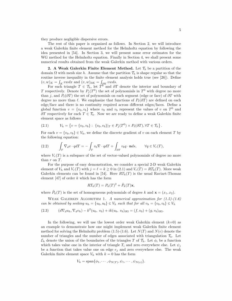
Fig. 4.4. WG solutions for the non-convex Helmholtz problem with k = 4 and ξ = 2/3. Left:Mesh level 1; Right: Mesh level 6.

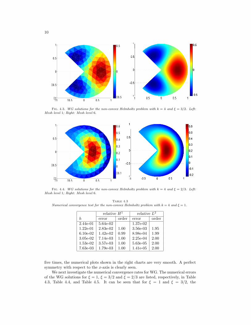
Table 4.3Numerical convergence test for the non-convex Helmholtz problem with k = 4 and ξ = 1.

relative H1 relative L2

h error order error order2.44e-01 5.64e-02 1.37e-021.22e-01 2.83e-02 1.00 3.56e-03 1.956.10e-02 1.42e-02 0.99 8.98e-04 1.993.05e-02 7.14e-03 1.00 2.25e-04 2.001.53e-02 3.57e-03 1.00 5.63e-05 2.007.63e-03 1.79e-03 1.00 1.41e-05 2.00

five times, the numerical plots shown in the right charts are very smooth. A perfectsymmetry with respect to the x-axis is clearly seen.

We next investigate the numerical convergence rates for WG. The numerical errorsof the WG solutions for ξ = 1, ξ = 3/2 and ξ = 2/3 are listed, respectively, in Table4.3, Table 4.4, and Table 4.5. It can be seen that for ξ = 1 and ξ = 3/2, the

11

Table 4.4Numerical convergence test for the non-convex Helmholtz problem with k = 4 and ξ = 3/2.

relative H1 relative L2

h error order error order2.44e-01 5.56e-02 1.12e-21.22e-01 2.81e-02 0.98 3.02e-03 1.896.10e-02 1.42e-02 0.99 8.06e-04 1.913.05e-02 7.14e-03 0.99 2.12e-04 1.921.53e-02 3.58e-03 1.00 5.54e-05 1.947.63e-03 1.79e-03 1.00 1.44e-05 1.95

Table 4.5Numerical convergence test for the non-convex Helmholtz problem with k = 4 and ξ = 2/3.

relative H1 relative L2

h error order error order2.44e-01 1.07e-01 5.24e-021.22e-01 5.74e-02 0.90 2.18e-02 1.276.10e-02 3.23e-02 0.83 9.01e-03 1.273.05e-02 1.89e-02 0.77 3.68e-03 1.291.53e-02 1.14e-02 0.73 1.49e-03 1.317.63e-03 6.99e-03 0.71 5.96e-04 1.32

numerical convergence rates in the relative H1 and L2 errors remain to be first andsecond order, while the convergence orders degrade for the non-smooth case ξ = 2/3.Mathematically, for both ξ = 3/2 and ξ = 2/3, the exact solutions (4.2) are known tobe non-smooth across the negative x-axis if the domain was chosen to be the entirecircle. However, the present domain excludes the negative x-axis. Thus, the sourceterm f of the Helmholtz equation (1.5) can be simply defined as zero throughout Ω.Nevertheless, there still exists some singularities at the origin (0, 0). In particular, itis remarked in [37] that the singularity lies in the derivatives of the exact solution at(0, 0). Due to such singularities, the convergence rates of high order DG methods arealso reduced for ξ = 3/2 and ξ = 2/3 [37]. In the present study, we further note thatthere exists a subtle difference between two cases ξ = 3/2 and ξ = 2/3 at the origin.To see this, we neglect the second cos(·) term in the exact solution (4.2) and plot theBessel function of the first kind Jξ(k|r|) along the radial direction r, see Fig. 4.5. It isobserved that the Bessel function of the first kind is non-smooth for the case ξ = 2/3,while it looks smooth across the origin for the case ξ = 3/2. Thus, it seems that thefirst derivative of J3/2(k|r|) is still continuous along the radial direction. This perhapsexplains why the present WG method does not experience any order reduction for thecase ξ = 3/2. In [37], locally refined meshes were employed to resolve the singularityat the origin so that the convergence rate for the case ξ = 2/3 can be improved.We note that local refinements can also be adopted in the WG method for a betterconvergence rate. A study of WG with grid local refinement is left to interested partiesfor future research.

4.3. A Helmholtz problem with inhomogeneous media. We consider aHelmholtz problem with inhomogeneous media defined on a circular domain withradius R. Note that the spatial function d(x, y) in the Helmholtz equation (1.5)

12

−0.1 −0.05 0 0.05 0.1

0

0.1

0.2

0.3

0.4

r

J ξ(k |r

|)

ξ=3/2ξ=2/3

Fig. 4.5. The Bessel function of the first kind Jξ(k|r|) across the origin.

represents the dielectric properties of the underlying media. In particular, we haved = 1

ε in the electromagnetic applications [56], where ε is the electric permittivity. Inthe present study, we construct a smooth varying dielectric profile:

(4.3) d(r) =1

ε1S(r) +

1

ε2(1− S(r)),

where r =√x2 + y2, ε1 and ε2 are dielectric constants, and

(4.4) S(r) =

1 if r < a,

−2(b−rb−a

)3

+ 3(b−rb−a

)2

if a ≤ r ≤ b,0 if r > b,

with a < b < R. An example plot of d(r) and S(r) is shown in Fig. 4.6. In classicalelectromagnetic simulations, ε is usually taken as a piecewise constant, so that somesophisticated numerical treatments have to be conducted near the material interfacesto secure the overall accuracy [56]. Such a procedure can be bypassed if one considersa smeared dielectric profile, such as (4.3). We note that under the limit b → a,a piecewise constant profile is recovered in (4.3). In general, the smeared profile(4.3) might be generated via numerical filtering, such as the so-called ε-smoothingtechnique [51] in computational electromagnetics. On the other hand, we note thatthe dielectric profile might be defined to be smooth in certain applications. Forexample, in studying the solute-solvent interactions of electrostatic analysis, somemathematical models [24, 57] have been proposed to treat the boundary between theprotein and its surrounding aqueous environment to be a smoothly varying one. Infact, the definition of (4.3) is inspired by a similar model in that field [24].

In the present study, we choose the source of the Helmholtz equation (1.5) to be

(4.5) f(r) = k2[d(r)− 1]J0(kr) + kd′(r)J1(kr),

where

(4.6) d′(r) =

(1

ε1− 1

ε2

)S′(r)

13

0 1 2 3 4 50

0.25

0.5

0.75

1

r

S(r)d(r)

Fig. 4.6. An example plot of smooth dielectric profile d(r) and S(r) with a = 1, b = 3 andR = 5. The dielectric coefficients of protein and water are used, i.e., ε1 = 2 and ε2 = 80.

and

(4.7) S′(r) =

0 if r < a,

6(b−rb−a

)2

− 6(b−rb−a

)if a ≤ r ≤ b,

0 if b < r,

For simplicity, a Dirichlet boundary condition is imposed at r = R with u = g. Hereg is prescribed according to the exact solution

(4.8) u = J0(kr).

Our numerical investigation assumes the value of a = 1, b = 3 and R = 5.The wave number is set to be k = 2. The dielectric coefficients are chosen as ε1 =2 and ε2 = 80, which represents the dielectric constant of protein and water [24,57], respectively. The WG method with piecewise constant finite element functionsis employed to solve the present problem with inhomogeneous media in Cartesiancoordinate. Table 4.6 illustrates the computational errors and some numerical rate ofconvergence. It can be seen that the numerical convergence in the relative L2 erroris not uniform, while the relative H1 error still converges uniformly in first order.This phenomena might be related to the non-uniformity and smallness of the mediain part of the computational domain. Nevertheless, the averaged convergence rate inthe relative L2 norm is about 2.12. Overall, we are confident that the WG method isaccurate and robust in solving the Helmholtz equations with inhomogeneous media.

4.4. Large wave numbers. We finally investigate the performance of the WGmethod for the Helmholtz equation with large wave numbers. The homogeneousHelmholtz problem studied in the Subsection 4.1 is employed again for this purpose.Also, the RT0 and RT1 elements are used to solve the homogeneous Helmholtz equa-tion with the Robin boundary condition. Since this problem is defined on a structuredhexagon domain, a uniform triangular mesh with a constant mesh size h throughoutthe domain is used. This enables us to precisely evaluate the impact of the meshrefinements. Following the literature works [12, 33], we will focus only on the relativeH1 semi-norm in the present study.

14

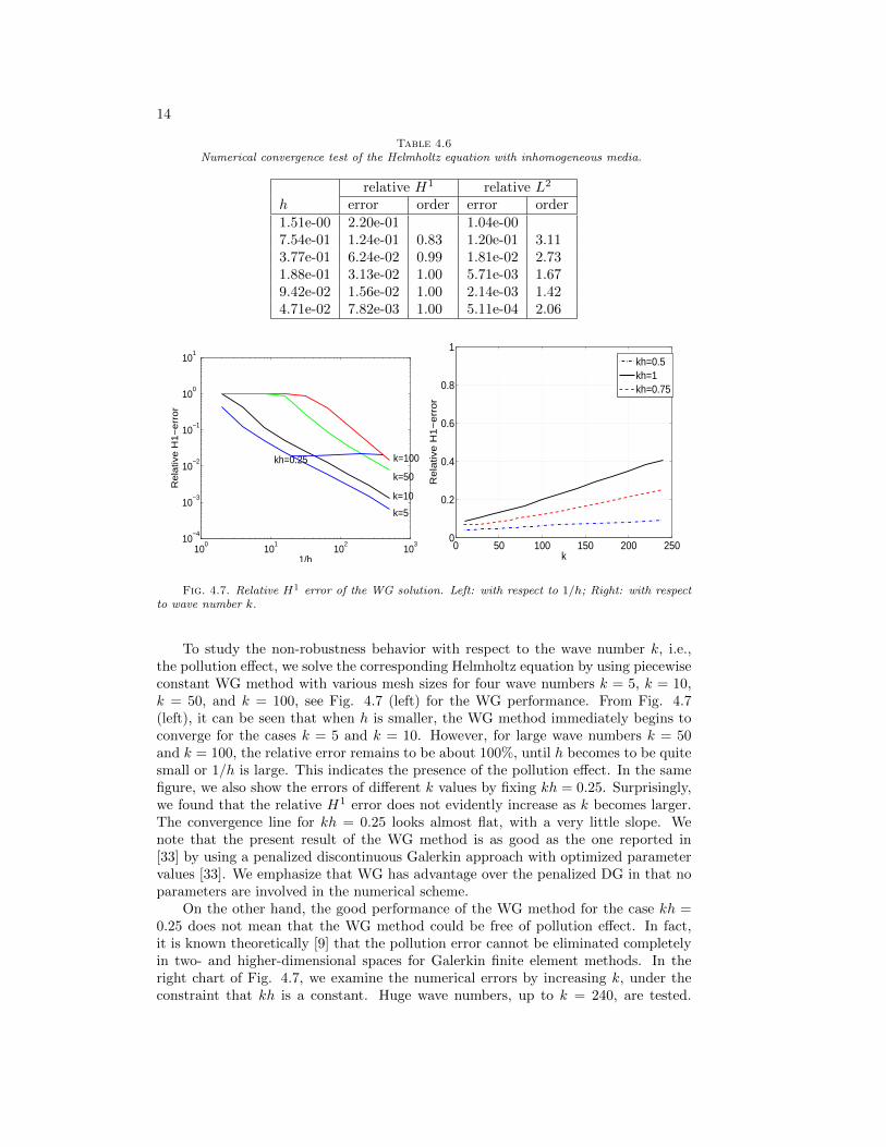
Table 4.6Numerical convergence test of the Helmholtz equation with inhomogeneous media.

relative H1 relative L2

h error order error order1.51e-00 2.20e-01 1.04e-007.54e-01 1.24e-01 0.83 1.20e-01 3.113.77e-01 6.24e-02 0.99 1.81e-02 2.731.88e-01 3.13e-02 1.00 5.71e-03 1.679.42e-02 1.56e-02 1.00 2.14e-03 1.424.71e-02 7.82e-03 1.00 5.11e-04 2.06

100

101

102

103

10−4

10−3

10−2

10−1

100

101

1/h

Re

lativ

e H

1−

err

or

k=100kh=0.25

k=50

k=5

k=10

0 50 100 150 200 2500

0.2

0.4

0.6

0.8

1

k

Rela

tive H

1−

err

or

kh=0.5kh=1kh=0.75

Fig. 4.7. Relative H1 error of the WG solution. Left: with respect to 1/h; Right: with respectto wave number k.

To study the non-robustness behavior with respect to the wave number k, i.e.,the pollution effect, we solve the corresponding Helmholtz equation by using piecewiseconstant WG method with various mesh sizes for four wave numbers k = 5, k = 10,k = 50, and k = 100, see Fig. 4.7 (left) for the WG performance. From Fig. 4.7(left), it can be seen that when h is smaller, the WG method immediately begins toconverge for the cases k = 5 and k = 10. However, for large wave numbers k = 50and k = 100, the relative error remains to be about 100%, until h becomes to be quitesmall or 1/h is large. This indicates the presence of the pollution effect. In the samefigure, we also show the errors of different k values by fixing kh = 0.25. Surprisingly,we found that the relative H1 error does not evidently increase as k becomes larger.The convergence line for kh = 0.25 looks almost flat, with a very little slope. Wenote that the present result of the WG method is as good as the one reported in[33] by using a penalized discontinuous Galerkin approach with optimized parametervalues [33]. We emphasize that WG has advantage over the penalized DG in that noparameters are involved in the numerical scheme.

On the other hand, the good performance of the WG method for the case kh =0.25 does not mean that the WG method could be free of pollution effect. In fact,it is known theoretically [9] that the pollution error cannot be eliminated completelyin two- and higher-dimensional spaces for Galerkin finite element methods. In theright chart of Fig. 4.7, we examine the numerical errors by increasing k, under theconstraint that kh is a constant. Huge wave numbers, up to k = 240, are tested.

15

It can be seen that when the constant changes from 0.5 to 0.75 and 1.0, the non-robustness behavior against k becomes more and more evident. However, the slopesof kh=constant lines remain to be small and the increment pattern with respect to kis always monotonic. This suggests that the pollution error is well controlled in theWG solution.

Fig. 4.8. Exact solution (left) and piecewise constant WG approximation (right) for k = 100,and h = 1/60.

In the rest of the paper, we shall present some numerical results for the WGmethod when applied to a challenging case of high wave numbers. In Fig. 4.8 and 4.10,the WG numerical solutions are plotted against the exact solution of the Helmholtzproblem. Here we take a wave number k = 100 and mesh size h = 1/60 which isrelatively a coarse mesh. With such a coarse mesh, the WG method can still capturethe fast oscillation of the solution. However, the numerically predicted magnitudeof the oscillation is slightly damped for waves away from the center when piecewiseconstant elements are employed in the WG method. Such damping can be seen in atrace plot along x-axis or y = 0. To see this, we consider an even worse case withk = 100 and h = 1/50. The result is shown in the first chart of Fig. 4.9. Wenote that the numerical solution is excellent around the center of the region, but itgets worse as one moves closer to the boundary. If we choose a smaller mesh sizeh = 1/120, the visual difference between the exact and WG solutions becomes verysmall, as illustrate in Fig. 4.9. If we further choose a mesh size h = 1/200, the exactsolution and the WG approximation look very close to each other. This indicates anexcellent convergence of the WG method when the mesh is refined. In addition tomesh refinement, one may also obtain a fast convergence by using high order elementsin the WG method. Figure 4.11 illustrates a trace plot for the case of k = 100 andh = 1/60 when piecewise linear elements are employed in the WG method. It can beseen that the computational result with this relatively coarse mesh captures both thefast oscillation and the magnitude of the exact solution very well.

5. Concluding Remarks. The numerical experiments indicate that the WGmethod as introduced in [54] is a very promising numerical technique for solving theHelmholtz equations with large wave numbers. This finite element method is robust,efficient, and easy to implement. On the other hand, a theoretical investigation for theWG method should be conducted by taking into account some useful features of theHelmholtz equation when special test functions are used. It would also be valuable to

16

−1 −0.5 0 0.5 1−0.1

−0.05

0

0.05

0.1k=100, h=1/50

Numerical solutionExact solution

−1 −0.5 0 0.5 1−0.1

−0.05

0

0.05

0.1k=100, h=1/120

Numerical solutionExact solution

−1 −0.5 0 0.5 1−0.1

−0.05

0

0.05

0.1k=100, h=1/200

Numerical solutionExact solution

Fig. 4.9. The trace plot along x-axis or y = 0 form WG solution using piecewise constants.

test the performance of the WG method when high order finite elements are employedto the Helmholtz equations with large wave numbers in two and three dimensionalspaces.

17

Fig. 4.10. Exact solution (left) and piecewise linear WG approximation (right) for k = 100,and h = 1/60.

−1 −0.5 0 0.5 1−0.1

−0.05

0

0.05

0.1k=100, h=1/60

Numerical solutionExact Solution

Fig. 4.11. The trace plot along x-axis or y = 0 form WG solution using piecewise linearelements.

18

REFERENCES

[1] M. Ainsworth, Discrete dispersion relation for hp-version finite element approximation athigh wave number, SIAM J. Numer. Anal., 42, pp. 553-575, 2004.

[2] M. Ainsworth, P. Monk, and W. Muniz, Dispersive and dissipative properties of discontin-uous Galerkin finite element methods for the second-order wave equation, J. Sci. Comput,27, pp. 5-40, 2006.

[3] M. Ainsworth and H.A. Wajid, Dispersive and dissipative behavior of the spectral elementmethod, SIAM J. Numer. Anal., 47, pp. 3910-3937, 2009.

[4] D. N. Arnold, An interior penalty finite element method with discontinuous elements, SIAMJ. Numer. Anal., 19(4), pp. 742-760, 1982.

[5] D. N. Arnold and F. Brezzi, Mixed and nonconforming finite element methods: imple-mentation, postprocessing and error estimates, RAIRO Modl. Math. Anal. Numr., 19(1),pp. 7-32, 1985.

[6] D. Arnold, F. Brezzi, B. Cockburn, and L. D. Marini, Unified analysis of discontinuousGalerkin methods for elliptic problems, SIAM J. Numer. Anal., 39 (2002), pp. 1749–1779.

[7] I. Babuska, The finite element method with Lagrange multipliers, Numer. Math., 20 (1973),pp. 179-192.

[8] I. Babuska, F. Ihlenburg, E.T. Paik, S.A. Sauter, A generalized finite element method for solvingthe Helmholtz equation in two dimensions with minimal pollution. Computer Methods inApplied Mechanics and Engineering 1995; 128: 325-359.

[9] I. Babuska, S.A. Sauter, Is the pollution effect of the FEM avoidable for the Helmholtz equationconsidering high wave number? SIAM Journal on Numerical Analysis 1997; 34: 2392-2423. Reprinted in SIAM Review 2000; 42: 451-484.

[10] I. Babuska, U. Banerjee, and J. Osborn, Generalized finite element method - main ideas, results,and perspective, Internat. J. Comput. Methods, 1 (2004), pp. 67-103.

[11] G. A. Baker, Finite element methods for elliptic equations using nonconforming elements,Math. Comp., 31 (1977), pp. 45-59.

[12] G. Bao, G.W. Wei, and S. Zhao, Numerical solution of the Helmholtz equation with highwavenubers, Int. J. Numer. Meth. Engng, 59 (2004), pp. 389-408.

[13] C. E. Baumann and J.T. Oden, A discontinuous hp finite element method for convection-diffusion problems, Comput. Methods Appl. Mech. Engrg., 175 (1999), pp. 311-341.

[14] S. Brenner and R. Scott, The Mathematical Theory of Finite Element Mathods, Springer-Verlag, New York, 1994.

[15] F. Brezzi, On the existence, uniqueness, and approximation of saddle point problems arisingfrom Lagrange multipliers, RAIRO, 8 (1974), pp. 129-151.

[16] F. Brezzi and M. Fortin, Mixed and Hybrid Finite Elements, Springer-Verlag, New York,1991.

[17] F. Brezzi, J. Douglas, Jr., R. Durn and M. Fortin, Mixed finite elements for second orderelliptic problems in three variables, Numer. Math., 51 (1987), pp. 237-250.

[18] F. Brezzi, J. Douglas, Jr., and L.D. Marini, Two families of mixed finite elements forsecond order elliptic problems, Numer. Math., 47 (1985), pp. 217-235.

[19] A. Buffa and P. Monk, Error Estimates for the ultra weak variational formulation of theHelmholtz equation, ESAIM: Mathematical Modelling and Numerical Analysis, 42 (2008),pp. 925-940.

[20] P. Castillo, B. Cockburn, I. Perugia, and D. Schotzau, An a priori error analysis ofthe local discontinuous Galerkin method for elliptic problems, SIAM J. Numer. Anal., 38(2000), pp. 1676-1706.

[21] O. Cessenat and B. Despres, Application of the ultra-weak variational formulation of ellipticPDEs to the 2-dimensional Helmholtz problem, SIAM J. Numer. Anal., 35 (1998), pp. 255-299.

[22] O. Cessenat and B. Despres, Using plane waves as base functions for solving time harmonicequations with the ultra weak varational formulation, J. Comput. Acoustics, 11 (2003),pp. 227-238.

[23] S.N. Chandler-Wilde and S. Langdon, A Galerkin boundary element method for high fre-quency scattering by convex polygons, SIAM J. Numer. Anal., 45 (2007), pp. 610-640.

[24] Z. Chen, N.A. Baker, and G.W. Wei, Differential geometry based solvation model I: Eulerianformulation, J. Comput. Phys., 229 (2010), pp. 8231-8258.

[25] E.T. Chung and B. Engquist, Optimal discontinuous Galerkin methods for wave propagation,SIAM J. Numer. Anal., 44 (2006), pp. 2131-2158.

[26] P.G. Ciarlet, The Finite Element Method for Elliptic Problems, North-Holland, New York,1978.

19

[27] B. Cockburn and C.-W. Shu, The local discontinuous Galerkin method for time-dependentconvection-diffusion systems, SIAM J. Numer. Anal., 35 (1998), pp. 2440-2463.

[28] B. Cockburn and C.-W. Shu, Runge-Kutta Discontinuous Galerkin methods for convection-dominated problems, Journal of Scientific Computing, 16 (2001), pp. 173-261.

[29] B. Cockburn, B. Dong, and J. Guzman, A superconvergent LDG-hybridizable Galerkinmethod for second-order elliptic problems, Math. COmput. 77 (2008), pp. 1887-1916.

[30] B. Cockburn, J. Gopalakrishnan, and R. Lazarov, Unified hybridization of discontinuousGalerkin, mixed and continuous Galerkin methods for second- order elliptic problems,SIAM J. Numer. Anal. 47 (2009), pp. 1319-1365.

[31] C. Harhat, I. Harari, and U. Hetmaniuk, A discontinuous Galerkin methodwith Lagrangemultiplies for the solution of Helmholtz problems in the mid-frequency regime, Comput.Methods Appl. Mech. Engrg., 192 (2003), pp. 1389-1419.

[32] C. Harhat, R. Tezaur, and P. Weidemann-Goiran, Higher-order extensions of a discontin-uous Galerkin method for mid-frequency Helmholtz problems, Int. J. Numer. Meth. Engng,61 (2004), pp. 1938-1956.

[33] X. Feng and H. Wu, Discontinuous Galerkin methods for the Helmholtz equation with largewave number, SIAM J. Numer. Anal., 47 (2009), pp. 2872-2896.

[34] B. X. Fraeijs de Veubeke, Displacement and equilibrium models in the finite element method,In “Stress Analysis”, O. C. Zienkiewicz and G. Holister (eds.), John Wiley, New York, 1965.

[35] B. X. Fraeijs de Veubeke, Stress function approach, International Congress on the FiniteElement Methods in Structural Mechanics, Bournemouth, 1975.

[36] E. Giladi, Asymptotically derived boundary elements for the Helmholtz equation in high fre-quencies, J. Comput. Appl. Math. 2007; 198, 52-74.

[37] R. Griesmaier and P. Monk, Error analysis for a hybridizable discontinuous Galerkin methodfor the Helmholtz equation, J. Sci. Comput. 2011; in press.

[38] I. Harari, T.J.R. Hughes, Finite element methods for the Helmholtz equation in an exteriordomain: model problems, Computer Methods in Applied Mechanics and Engineering 1991;87: 59-96.

[39] E. Heikkola, S. Monkola, A. Pennanen, and T. Rossi, Controllability method for the Helmholtzequation with higher-order discretizations. J. Comput. Phys. 2007; 225: 1553-1576.

[40] F. Ihlenburg, I. Babuska, Dispersion analysis and error estimation of Galerkin finite elementmethods for the Helmholtz equation. International Journal for Numerical Methods in En-gineering 1995; 38: 3745-3774.

[41] F. Ihlenburg, I. Babuska, Finite element solution of the Helmholtz equation with high wavenum-ber Part I: the h-version of the FEM. Computer and Mathematics with applications 1995;30: 9-37.

[42] F. Ihlenburg, I. Babuska, Finite element solution of the Helmholtz equation with high wavenum-ber Part II: the h-p-version of the FEM. SIAM Journal of Numerical Analysis 1997; 34:315-358.

[43] Y. Jeon, and E. Park, A Hybrid Discontinuous Galerkin Method for Elliptic Problems, SIAMJ. Numer. Anal. 48 (2010), pp. 1968-1983.

[44] S. Langdon and S.N. Chandler-Wilde, A wavenumber independent boundary elementmethod for an accoustic scattering problem, SIAM J. Numer. Anal., 43 (2006), pp. 2450-2477.

[45] J.M. Melenk and I. Babuska, The partition of unity finite element method: Basic theory andapplications, Comput. Methods Appl. Mech. Engrg. 139, (1996), pp. 289-314.

[46] P. Monk and D.Q. Wang, A least-squares method for the Helmholtz equation, Comput. Meth-ods Appl. Mech. Engrg. 175, (1999), pp. 121-136.

[47] P. Raviart and J. Thomas, A mixed finite element method for second order elliptic prob-lems, Mathematical Aspects of the Finite Element Method, I. Galligani, E. Magenes, eds.,Lectures Notes in Math. 606, Springer-Verlag, New York, 1977.

[48] B. Riviere, M. F. Wheeler, and V. Girault, A priori error estimates for nite element meth-ods based on discontinuous approximation spaces for elliptic problems, SIAM J. Numer.Anal., 39 (2001), pp. 902-931.

[49] B. Riviere, M. F. Wheeler, and V. Girault, Improved Energy Estimates for InteriorPenalty, Constrained and Discontinuous Galerkin Methods for Elliptic Problems. PartI, Computational Geosciences , volume 8 (1999), pp. 337-360.

[50] A. H. Schatz, An observation concerning Ritz-Galerkin methods with indefinite bilinear forms,Math. Comp., 28 (1974), pp. 959-962.

[51] Z.H. Shao, G.W. Wei and S. Zhao, DSC time-domain solution of Maxwell’s equations, J.Comput. Phys., 189 (2003), pp. 427-453.

[52] J. Shen and L.-L. Wang, Spectral approximation of the Helmholtz equation with high wave

20

numbers, SIAM J. Numer. Anal., 43 (2005), pp. 623-644.[53] J. Shen and L.-L. Wang, Analysis of a spectral-Galerkin approximation to the Helmhotlz

equation in exterior domains, SIAM J. Numer. Anal., 45 (2007), pp. 1954-1978.[54] J. Wang and X. Ye, A weak Galerkin finite element method for second-order elliptic problems,

Preprint submitted to SINUM, 2011.[55] J. Wang, Mixed finite element methods, Numerical Methods in Scientific and Engineering

Computing, Eds: W. Cai, Z. Shi, C-W. Shu, and J. Xu, Academic Press.[56] S. Zhao, High order matched interface and boundary methods for the Helmholtz equation in

media with arbitrarily curved interfaces, J. Comput. Phys., 229 (2010), pp. 3155-3170.[57] S. Zhao, Pseudo-time coupled nonlinear models for biomolecular surface representation and

solvation analysis, Int. J. Numer. Methods Biomedical Engrg., (2011), in press.[58] O.C. Zienkiewicz, Achievements and some unsolved problems of the finite element method.

International Journal for Numerical Methods in Engineering 2000; 47: 9-28.