A one-dimensional computational model for the interaction ...

A one-dimensional computational model for the interaction ofphase-transformations and plasticity

Richard Ostwalda,∗, Thorsten Bartela, Andreas Menzela,b

aInstitute of Mechanics, TU Dortmund, Leonhard-Euler-Str. 5, D-44227 Dortmund, GermanybDivision of Solid Mechanics, Lund University, P.O. Box 118, SE-22100 Lund, Sweden

Abstract

In this work, we model the basic mechanisms of the interaction between phase-transformations and plasticitywithin a one-dimensional constitutive framework. Efficient algorithms are presented, facilitating to solve theunderlying evolution equations with high numerical stability at low numerical costs. Furthermore, a family offunctions covering physically reasonable classes for the inheritance of plasticity in the context of evolving phasesis proposed and discussed by means of several representative numerical examples.

Key words: Phase-transformations, Plasticity, Mixture-theory

1. Introduction

Functional materials like TRIP-steels and shape memory alloys offer a great potential for the industrialmanufacturing of sophisticated components benefitting from the advantages that these materials can provide,such as locally varying hardness and stiffness. The need of a reliable manufacturing and application of suchcomponents leads to the demand of accurate constitutive models not only to predict the material’s response bymeans of simulations, but also in view of material and structural design purposes. However, the coupling ofphase-transformations and plasticity involves the interaction of multiple complex physical mechanisms, whichhave not yet been completely understood.

Micromechanically motivated material models are characterized by considering the microstructure of a mate-rial and its stress- or temperature-driven evolution. As shown in Bain (1924) and Bowles and MacKenzie (1954),in particular the kinematics of martensitic (i.e. diffusionless) solid-solid phase-transformations are characterizedby homogeneous deformations of the crystal lattice. Thus, the transformation kinematics can be captured byso-called Bain-strains represented for example by the right stretch tensor U tr in a continuum mechanical context(see for example James and Hane (2000); Bhattacharya (2003)). Besides that, the material’s microstructure canbe approximately accounted for by matrix-inclusion homogenization schemes as suggested in Sun et al. (1991);Sun and Hwang (1993); Cherkaoui et al. (2000). These schemes approximate effective material properties for thephase mixture being bounded by the Voigt and Reuss limits, respectively. In this regard, a promising methodfor the determination of a suitable effective material response is referred to as energy relaxation.

The concept of energy relaxation is dedicated to the computation of the quasiconvex energy hull of anunderlying multi-well free energy potential. It offers the possibility to predict the energetically most favorablearrangement of the underlying microstructure. A comprehensive treatise on quasiconvex analysis can be found

∗Corresponding author. Email: [email protected]

INTERNATIONAL JOURNAL OF STRUCTURAL CHANGES IN SOLIDS – Mechanics and Applications Volume 3, Number 1, February 2011, pp. 63-82

64 Ostwald et al. / International Journal of Structural Changes in Solids 3(2011) 63-82

in Morrey (1952); Ball (1977); Dacorogna (1989) among others. Since the exact determination of the desiredenergy hull is only possible in rare cases as e.g. shown in Kohn (1991); DeSimone and Dolzmann (1999), thequasiconvexification is mostly approximated by upper and lower bounds as shown in Pagano et al. (1998); Ortizand Repetto (1999); Stupkiewicz and Petryk (2002); Miehe et al. (2004). An extension of the energy relaxationconcept has recently been presented in Bartel and Hackl (2009), where the deformations within each phase aredirectly derived from a superimposed displacement fluctuation field. Moreover, a distinction between elastic anddissipative internal variables is introduced therein in order to, on the one hand, determine a well-suited energyhull while, on the other hand, being able to account for the hysteretic behaviour of shape memory alloys. In thiscontext, the evolution of dissipative variables can be established by ordinary differential equations derived frominelastic potentials according to e.g. Mielke and Theil (1999); Mielke et al. (2002).

The mentioned micromechanically motivated models are mainly based on the minimization of total energyand total power, respectively. In contrast to this, the models presented in Berezovski and Maugin (2007); Mauginand Berezovski (2009); Abeyaratne and Knowles (1990, 1993, 1997) are based on the derivation of driving forcesdirectly acting on the propagating phase front. However, the increase of accuracy and physical plausiblity enabledby micromechanical models is always accompanied by a significant increase of computational effort. In particular,the determination of energetically favorable arrangements of phases subjected to compatibility conditions (rank-one connections) leads to immense numerical costs. Moreover, micromechanical models are usually capableof simulating the behaviour of single crystals—in order to extend these models to polycrystalline materials,appropriate scale-bridging methods are required. Thus, the computation of large macroscopic problems—forexample in the context of finite element simulations—is often realized using phenomenological approaches. Theseapproaches, as for example introduced in Helm and Haupt (2003); Auricchio and Taylor (1997); Raniecki et al.(1992), are mainly based on thermodynamics. In addition to the first and second law of thermodynamics, theconcept of generalized irreversible forces and fluxes, as established in Truesdell and Toupin (1960) amongstothers, is used in order to derive evolution equations for the internal variables. An extension of the modelproposed in Raniecki et al. (1992) has been presented in Muller and Bruhns (2006) in terms of finite strains anda self-consistent Eulerian theory accounting for heat generation during phase-transformations.

Another class of thermodynamical models is related to statistical considerations, resulting in transformationprobabilities. As for example elaborated in Achenbach (1989); Abeyaratne and Knowles (1993); Huo and Muller(1993); Abeyaratne et al. (1994); Seelecke (1996); Muller and Seelecke (2001), these models are based on multi-well Helmholtz free energy potentials. The nucleation criteria are formulated in terms of energy barriers, whichlead to statistically derived transformation probabilities governing—together with Boltzmann-based transitionattempt frequencies, see e.g. Govindjee and Hall (2000)—the evolution of material phases.

The goal of this contribution is to enhance the statitics-based phase-transformation model described in Govin-djee and Hall (2000); Ostwald et al. (2010) in order to take into account plasticity as well as the interactionbetween phase-transformation and plasticity effects by introducing a so-called plastic inheritance law. The modelis presented in Section 2, where extended Helmholtz free energy functions for each material phase are presented,taking into account plastic strains as new variables for each individual phase. Based on the extended multi-wellenergy potentials, the probabilistic phase-transformation model is derived in Section 2.1. Moreover, the differ-ential equations describing the evolution of plasticity as well as the potential-based derivation of the individualplastic driving forces are shown in Section 2.2 and 2.2.1, respectively. The coupling of phase-transformation andplasticity effects is incorporated by means of a staggered algorithm. To this end, an inheritance algorithm for theinheritance of plastic strains resulting from a propagating phase front is introduced in Section 2.3. Moreover, twophysically reasonable exponential-type inheritance probability functions are presented in Section 2.3.1 and 2.3.2.Details on the numerical implementation of the model are provided in Section 3, followed by numerical examplesshown in Section 4, where the model is applied not only to shape memory alloys (see Section 4.2), but also toTRIP steel (see Section 4.3). It is shown that the model nicely reflects the actual physical behaviour of bothtypes of materials.

Ostwald et al. / A model for the interaction of phase-transformations and plasticity 65

2. A model for the interaction of phase-transformations and plasticity

The one-dimensional phase-transformation model is based on mixture theory, where we make use of the Voigtassumption, i.e. all material phases are subject to the same strain ε. The implemented phase-transformationmodel is capable of handling an arbitrary amount of material phases, where the volume fraction

ξαdef= lim

v→0

(vα

v

)(1)

of each phase α ∈ {1, . . . , ν} ⊂ N is subject to the restrictions

ξα ∈ [0, 1] ⊂ R ,∑α

ξα = 1 ,∑α

ξα = 0 . (2)

While the validity of (2)a and (2)b is evident, (2)c follows from mass conservation. Each phase is presumed tobehave thermo-elasto-plastically, thus a Helmholtz free energy function ψα = ψα(ε, εαpl, θ) of the form

ρ0ψα =

12Eα[ε− εαtr − εαpl]

2 − ζαEα[ε− εαtr − εαpl][θ − θ0]

+ ρ0cαp θ

[1− log

(θ

θ0

)]− ρ0λ

αT

[1− θ

θ0

](3)

is assigned to each phase α, with E the Young’s modulus, ε = ∇xu the total strains, εtr the transformationstrains, εpl the plastic strains, ζ the coefficient of thermal expansion, θ the current absolute temperature, θ0the reference temperature, cp the heat capacity, and λT the latent heat of the respective material phase. Theoverall free energy of the mixture Ψ = Ψ(ε, ε1d

pl , θ, ξ) =∑α ξ

αψα, with ξ = [ξ1, . . . , ξν ] and ε1dpl = [ε1pl, . . . , ε

νpl],

can directly be obtained from the free energy contributions of the respective constituents, since the distortionalenergy of the phase boundaries is neglected here.

Based on this, the Gibbs potential G = G(∂Ψ/∂ε, ξ, θ) can be obtained by carrying out a Legendre-transformation, i.e.

G = − supε

⎛⎝ ∂Ψ(ε, ε1dpl , θ, ξ)∂ε

∣∣∣∣∣θ,ε1d

pl

ε− ρ0Ψ

⎞⎠ (4)

= − supε

(∑α

ξα [σε− ρ0ψα]

)(5)

= − supε

(∑α

ξαgα

), (6)

where σ = ∂Ψ/∂ε|θ,ε1dpl

= σ(ε, ε1dpl , ξ, θ) is the stress acting in the one-dimensional continuum considered and

gα = g α(σ, ε, εαpl, θ)def= σε− ρ0ψ

α represents the contribution of phase α to the overall Gibbs potential G.

2.1. Evolution of volume fractionsFor the evolution of the volume fractions ξα we use an approach based on statistical physics. In this regard,

a transformation probability matrix Qν ∈ Rν×ν introduced in Govindjee and Hall (2000) is used, facilitating to

derive the evolution of volume fractions as

ξ = Qν · ξ , (7)

wherein the notation • denotes the material time derivative. Since we restrict ourselves to two material phases inthis work, namely austenite (A) and martensite (M), the according transformation probability matrix Q2 ∈ R

2×2

reduces to

Q2 = ω

[−PA→M PM→A

PA→M −PM→A

]�= Qt

2 (8)


with ω the transition attempt frequency and Pα→β = Pα→β(θ, bα→β) the probability of a transformation of onephase α to the other phase β. Note that (8) refers to ξ = [ξA, ξM]t ∈ R

2. Furthermore,∑

iQij = 0 ∀ j guaranteesthat (2)c is fulfilled.

According to Achenbach (1989), the transformation probabilities necessary to assemble Q• can be obtainedfrom

Pα→β = exp(−Δv bα→β

k θ

), (9)

with Δv the constant transformation region’s volume, bα→β the energy barrier for the transformation from phaseα to phase β, k the Boltzmann’s constant, and θ the given temperature. Note that, in general, bα→β �= bβ→α

and thus Pα→β �= Pβ→α holds. The energy barriers can be determined from

bα→β = g α(σ, ε�α,β , θ)− g α(σ, εminα , θ) (10)

with

ε�α,β = infgα,gβ

{ε | g α(σ, ε, θ)|σ,θ = g β(σ, ε, θ)|σ,θ

}(11)

and

εminα =

{ε | ∂g

α(σ, ε, θ)∂ε

∣∣∣∣σ,θ

= 0

}, (12)

where g α(σ, ε�α,β , θ) = g β(σ, ε�α,β , θ) gives the value of the energy potentials at the intersection of the parabolicphase potential functions for two material phases (α, β) in strain space, while g α(σ, εmin

α , θ) denotes the minimumenergy potential of a particular phase α for fixed stresses and temperature. Accordingly, the difference of bothenergy values (10) gives the energy barrier that has to be overcome for a transformation from phase α to β.

2.2. Evolution of plastic strainsTo incorporate plasticity, we—for conceptual simplicity—assume von Mises-type plasticity with linear pro-

portional hardening. Based on the overall free energy potential, the plastic driving force qαpl,Ψ can be derived foreach phase α, see Section 2.2.1 for details. With the driving force and the current yield stress Y α at hand, theyield function Φα = Φα(Y α, qαpl,Ψ ) determining the admissible elastic domain in phase α, is given as

Φα(qαpl,Ψ , Yα) = |qαpl,Ψ − ξαbα| − ξα Y α ≤ 0 . (13)

The current yield stress Y α = Y α(γα) = Y α0 + Hα γα is given by the initial yield stress Y α0 being modified byHα γα due to accumulated plastic strains γα of the respective material phase, where Hα denotes the constanthardening modulus of phase α. The individual back stress ξαbα is additionally considered in order to preventplastic flow occurring in the initial equilibrium state. To be specific, the underlying Voigt assumption leads toan initial stress of

bαdef= σ α(ε = 0, εαpl = 0, θ)

=∂ψα(ε, εαpl, θ)

∂ε

∣∣∣∣∣θ,εα

pl=0,ε=0

= −Eαεαtr + ζαEαεαtr[θ − θ0] (14)

that acts in each phase α and, in consequence, is considered as a back stress in the yield function. Based on theyield function presented, we make use of an associated flow rule, facilitating to derive the evolution law for theplastic strain in phase α by means of

εαpl = λα∂Φα(qαpl,Ψ , Y

α)∂qαpl,Ψ

= λα sgn(qαpl,Ψ − ξαbα

)(15)

with an appropriate Lagrangian multiplier λα.


2.2.1. Remarks on the derivation of the plastic driving forceThe stress-type force qαpl,Ψ = q αpl,Ψ (ξα, ε, εαpl, θ) driving the evolution of plasticity in phase α can be derived

from the overall free energy Ψ according to

qαpl,Ψ = −∂Ψ(ε, ε1dpl , θ, ξ)

∂εαpl

∣∣∣∣∣θ,ε,ξ

(16)

= − ∂

∂εαpl

∣∣∣∣∣θ,ε

∑α

ξαψα(ε, εαpl, θ) (17)

= −ξα ∂ψα(ε, εαpl, θ)∂εαpl

∣∣∣∣∣θ,ε

, (18)

finally resulting in

qαpl,Ψ = ξα[Eα[ε− εαtr − εαpl] + ζαEα[θ − θ0]

]. (19)

Furthermore, the stress acting in the one-dimensional continuum is obtained from

σ =∂Ψ(ε, ε1d

pl , θ, ξ)∂ε

∣∣∣∣∣θ,ε1d

pl

(20)

=∂

∂ε

∣∣∣∣θ,ε1d

pl

[∑α

ξαψα(ε, εαpl, θ)

](21)

=∑α

ξα∂ψα(ε, εαpl, θ)

∂ε

∣∣∣∣∣θ,εα

pl

(22)

=∑α

ξασα (23)

with σα = σα(ε, εαpl, θ) = Eα[ε− εαtr − εαpl] + ζαEα[θ − θ0] the stress acting in phase α. Comparing this result to(19) shows that qαpl,Ψ = ξασα.

Alternatively, the plastic driving forces can be derived by considering each phase individually. Using thisapproach, the driving force qαpl,ψ = q αpl,ψ(ε, εαpl, θ) yields

qαpl,ψ = − ∂ψα(ε, εαpl, θ)∂εαpl

∣∣∣∣∣θ,ε

(24)

= Eα[ε− εαtr − εαpl] + ζαEα[θ − θ0] (25)= σα . (26)

In particular, this result leads to qαpl,Ψ = ξαqαpl,ψ. Note that the consideration of the volume fraction ξα withinthe plastic driving force of each phase α guarantees that q αpl,Ψ (ξα = 0, ε, εαpl, θ) = 0, and thus εαpl = 0 as long asξα = 0, i.e. no evolution of plasticity can occur within a phase of zero volume fraction.

2.3. Plastic inheritance

When the phase front of a phase α evolves throughout a crystal from time step nt to n+1t, the question arises,whether plastic strains present in the decreasing phase β are inherited by the phase front of the increasing phaseor not (see Figure 1). Conceptually speaking, one has to specify to which amount a positive volume fractionincrement Δξα = n+1ξα − nξα > 0 of phase α transfers plastic strains from phase β to phase α. In general, the


updated plastic strains εαpl = εαpl(nξα,Δξα, εαpl, ε

βpl, Π

β→α) in phase α can be determined via

εαpl =1

n+1ξα

[nξα εαpl +Πβ→αΔξα εβpl

], (27)

where Πβ→α reflects the probability of phase α inheriting the dislocations present in phase β (see Figure 1).If one further assumes, that the diffusionless lattice shearing taking place during the phase-transformationsconsidered neither generates nor annihilates any dislocations, i.e. the overall amount of plastic deformationsremains constant in terms of

n+1ξα εαpl + n+1ξβ εβpl = nξα εαpl + nξβ εβpl , (28)

then the updated plastic deformations εβpl = ε βpl(nξβ ,Δξα, εβpl, Π

β→α) remaining in the decreased phase β areobtained from

εβpl =1

n+1ξβ[nξβ −Πβ→αΔξα

]εβpl . (29)

As we restrict ourselves, for the sake of simplicity, to two phases, it is obvious that the increase Δξα of phaseα is related to the decrease Δξβ of phase β via

Δξβ = n+1ξβ − nξβ = −Δξα , Δξβ < 0 (30)

due to mass conservation, thus leading to

n+1ξβ = nξβ −Δξα . (31)

Comparing (29) and (31) then shows that, in case of Πβ→α = 1, the plastic deformations in the decreasing phase

are not affected by the change of volume fractions, i.e. ε βpl(nξβ ,Δξα, εβpl, Π

β→α = 1) = εβpl. On the other hand,in case of Πβ→α = 0, i.e. if all dislocations are pushed rather than inherited by the propagating phase front ofphase α, the plastic strains in phase β increase inversely proportional to the decrease of volume fraction.

However, it is physically reasonable to assume that the inheritance probability is not constant, but rather afunction depending on the remaining volume fraction ξβ and plastic strain εβpl of the decreasing phase β, as wellas on further material parameters characterizing the actual functional dependency. To this end, two reasonableapproaches for introducing exponential-type inheritance probability functions, namely a convex and a concaveone, Πβ→α

cvx = Πβ→αcvx (ξβ , εβpl;κ) and Πβ→α

ccv = Πβ→αccv (ξβ , εβpl;κ, ε

βpl,sat), respectively, are presented in the following.

2.3.1. Convex inheritance probability functionThe inheritance probability function considered is subjected to two physically reasonable restrictions. First,

in case that the volume fraction of the decreasing phase β is very large, i.e. ξβ ≈ 1, a propagating phase frontof phase α will most likely push dislocations present in phase β, since the dislocation density1—being inverselyproportional to the volume fraction—in β is rather low in this case. In consequence and as the first condition,we require the inheritance probability function to match Πβ→α

cvx (ξβ = 1, εβpl;κ) = 0. On the other hand, if theremaining volume fraction ξβ of the decreasing phase β tends to zero, the dislocation density takes high valuesso that the dislocations (or rather plastic strains) remaining in phase β are forced to be inherited by the evolvingphase α, i.e. Πβ→α

cvx (ξβ = 0, εβpl;κ) = 1. One exponential-type ansatz for an inheritance probability functionfulfilling these restrictions is

Πβ→αcvx (ξβ , εβpl;κ) = [1− ξβ ] exp

(−κ ξβ|εβpl|

). (32)

1The phrase dislocation density does not refer to curl(εpl), respectively ∂xεpl here. In the current context, we rather use thisdenomination as a synonym for the density of plastic strains.


α β

(a) Initial state: the phase front of α is about to move.

α β

(b) Πβ→α = 0, i.e. all dislocations are pushed by the phase-front and remainwithin phase β.

α β

(c) Πβ→α = 1, i.e. all dislocations within the volume that undergoes a phase-change are inherited to the growing phase α.

Figure 1: Dislocations can either be inherited or pushed by the propagating phase front of an evolvingphase α. Here, the two special cases, i.e. no inheritance (b) and full inheritance (c) of dislocationsduring phase front propagation are shown. However, the actual physical behaviour of a materialregarding inheritance of dislocations—or rather plastic strains—can be expected to lie in between bothextreme cases. Therefore an inheritance probability function Πβ→α = Πβ→α(ξβ , εβpl; ...) ∈ [0, 1] ⊂ R,depending on the volume fraction ξβ and plastic strain εβpl of phase β as well as on material parameters,is introduced in this work (see Sections 2.3.1 and 2.3.2).


Πβ→αcvx (ξβ , εβpl;κ = 0.1)

ξβεβpl

00 0

0.010.02

0.030.04

0.05

0.2

0.2

0.4

0.4

0.6

0.6

0.8

0.8

1

1

Πβ→αcvx (ξβ , εβpl = 0.025;κ)

κξβ

00

00.05

0.10.15

0.2

0.2

0.2

0.4

0.4

0.6

0.6

0.8

0.8

1

1

Figure 2: Convex inheritance probability function depending on volume fraction ξβ and plastic strainεβpl for given parameter κ = 0.1 (left), and the function depending on ξβ and κ for given plastic strainεβpl = 0.025 (right).

For an exemplary material parameter κ = 0.1, the development of this inheritance function is visualized inFigure 2. Besides that, the influence of the parameter κ for an exemplary fixed plastic strain of εβpl = 0.025 isdisplayed. As the figure shows, the proposed family of parametric inheritance functions is convex in ξ for allparameters κ ∈ R

+.

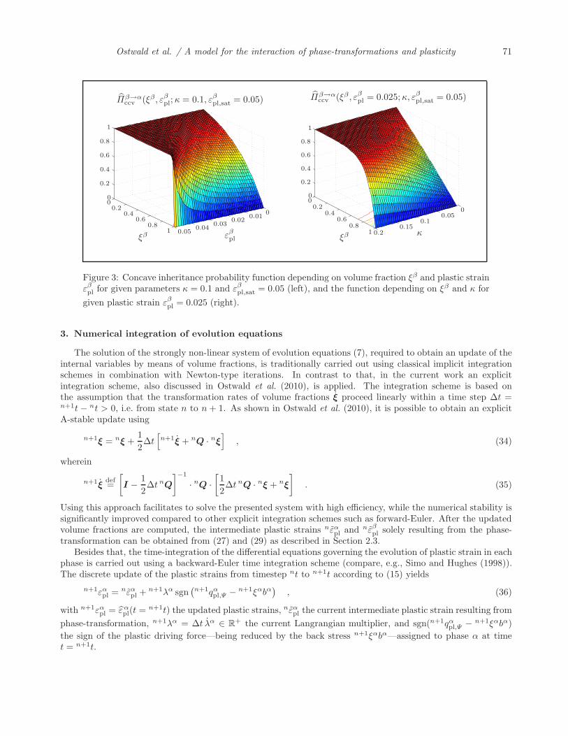
2.3.2. Concave inheritance probability functionAs an addition to the convex2 inheritance probability function shown in Section 2.3.1, a concave2 exponential-

type inheritance function is presented in the following. As before, the physical restrictions, i.e. Πβ→αccv (ξβ =

1, εβpl;κ) = 0 and Πβ→αccv (ξβ = 0, εβpl;κ) = 1, are required to be fulfilled. To be specific, the function

Πβ→αccv (ξβ , εβpl;κ, ε

βpl,sat) =

1− exp

(−κ [1− ξβ ]εβpl,sat − |εβpl|

)

1− exp

(−κ

εβpl,sat − |εβpl|

) , (33)

which again depends on a material parameter κ ∈ R+, is of exponential type, but provides a concave behaviour

in ξ. As above, we require the inheritance probability to increase with increasing plastic strain. Accordingly, aplastic saturation strain εβpl,sat ∈ R

+, which can also be regarded as a material-dependent quantity, is introducedhere. If the magnitude |εβpl| of the plastic strain present in phase β reaches the saturation strain εβpl,sat, theinheritance probability tends towards 1, i.e. Πβ→α

ccv (ξβ , εβpl → εβpl,sat;κ, εβpl,sat)→ 1 ∀ ξβ < 1. Figure 3 shows the

development of the concave inheritance function for a given parameter of κ = 0.1 and an exemplary saturationstrain of εβpl,sat = 0.05. Furthermore, the actual influence of κ on the inheritance probability function is presentedfor an exemplary plastic strain of εβpl = 0.025.

2Here and in the following, by convex or concave inheritance functions, we mean convex or concave in ξ.


Πβ→αccv (ξβ , εβpl;κ = 0.1, εβpl,sat = 0.05)

ξβ εβpl

00

00.01

0.020.03

0.040.05

0.2

0.2

0.4

0.4

0.6

0.6

0.8

0.8

1

1

Πβ→αccv (ξβ , εβpl = 0.025;κ, εβpl,sat = 0.05)

κξβ

00

00.05

0.10.15

0.2

0.2

0.2

0.4

0.4

0.6

0.6

0.8

0.8

1

1

Figure 3: Concave inheritance probability function depending on volume fraction ξβ and plastic strainεβpl for given parameters κ = 0.1 and εβpl,sat = 0.05 (left), and the function depending on ξβ and κ forgiven plastic strain εβpl = 0.025 (right).

3. Numerical integration of evolution equations

The solution of the strongly non-linear system of evolution equations (7), required to obtain an update of theinternal variables by means of volume fractions, is traditionally carried out using classical implicit integrationschemes in combination with Newton-type iterations. In contrast to that, in the current work an explicitintegration scheme, also discussed in Ostwald et al. (2010), is applied. The integration scheme is based onthe assumption that the transformation rates of volume fractions ξ proceed linearly within a time step Δt =n+1t − nt > 0, i.e. from state n to n+ 1. As shown in Ostwald et al. (2010), it is possible to obtain an explicitA-stable update using

n+1ξ = nξ +12Δt[n+1ξ + nQ · nξ

], (34)

wherein

n+1ξdef=[I − 1

2Δt nQ

]−1

· nQ ·[12Δt nQ · nξ + nξ

]. (35)

Using this approach facilitates to solve the presented system with high efficiency, while the numerical stability issignificantly improved compared to other explicit integration schemes such as forward-Euler. After the updatedvolume fractions are computed, the intermediate plastic strains nεαpl and nεβpl solely resulting from the phase-transformation can be obtained from (27) and (29) as described in Section 2.3.

Besides that, the time-integration of the differential equations governing the evolution of plastic strain in eachphase is carried out using a backward-Euler time integration scheme (compare, e.g., Simo and Hughes (1998)).The discrete update of the plastic strains from timestep nt to n+1t according to (15) yields

n+1εαpl = nεαpl + n+1λα sgn(n+1qαpl,Ψ − n+1ξαbα

), (36)

with n+1εαpl = εαpl(t = n+1t) the updated plastic strains, nεαpl the current intermediate plastic strain resulting fromphase-transformation, n+1λα = Δt λα ∈ R

+ the current Langrangian multiplier, and sgn(n+1qαpl,Ψ − n+1ξαbα)the sign of the plastic driving force—being reduced by the back stress n+1ξαbα—assigned to phase α at timet = n+1t.


In the current context, the Lagrangian multiplier can be expressed in terms of the trial value of the yieldfunction Φαtri = Φα(qαpl,Ψ,tri,

nY α), with the trial plastic driving force qαpl,Ψ,tri and nY α = Y α(nγα) the yield stressof phase α at time t = nt. For the derivation of the trial plastic driving force, we make use of the intermediatestate potential Ψ def= Ψ(n+1ε, nε1d

pl , θ,n+1ξ), where the updated volume fractions n+1ξ obtained from the phase-

transformation algorithm, (34) and (35), are considered. Thus, the trial plastic driving force for phase α resultsin

qαpl,Ψ,tri = −∂Ψ(n+1ε, nε1dpl , θ,

n+1ξ)∂ nεαpl

∣∣∣∣∣θ

= − ∂

∂ nεαpl

∣∣∣∣∣θ

∑α

n+1ξαψα(n+1ε, nεαpl, θ)

= −n+1ξα∂ψα(n+1ε, nεαpl, θ)

∂ nεαpl

∣∣∣∣∣θ

. (37)

Based on this, the trial value Φαtri of the yield function can be evaluated, facilitating to express the Lagrangianmultiplier as

n+1λα =Φαtri

n+1ξα [Eα +Hα]. (38)

The plastic strains εαpl in each phase α can then be updated from time nt to n+1t in an explicit manner accordingto (36), while the accumulated plastic strains n+1γα are obtained from

n+1γα = nγα + n+1λα . (39)

Here, the consistency of history variables is accounted for by considering the intermediate accumulated plasticstrains

nγα = γα(nγα, nεαpl,nεαpl)

def= nγα + |nεαpl − nεαpl| . (40)

Moreover, note that the change of plastic strains due to inheritance can be expressed in terms of

Δεαpl,inhdef= εαpl − εαpl . (41)

A flowchart visualizing the actual algorithmical implementation is provided in Appendix A in terms of a Nassi-Shneiderman diagramme.

4. Numerical Examples

This section provides several numerical examples for the model presented in Section 2, where we considerhomogeneous deformation states at constant temperature using a quasi-static strain rate of ε = 10−4 s−1. In Sec-tion 4.1 we show the behaviour of the phase-transformation model without consideration of plasticity, illustratingthat the implemented phase transformation model works correctly.

Then, in Section 4.2 the interactions between phase-transformations and plasticity are evaluated. In partic-ular, two numerical examples are adressed, highlighting the influence of concave and convex plastic inheritancefunctions. For these examples we restrict ourselves to the tensile regime in stress space, since we in this workonly consider a martensitic tension phase for simplicity.

In Section 4.3 we investigate the behaviour of the phase-transformation-plasticity model when applied tomaterial parameters corresponding to TRIP steel (see Table 2). Note that TRIP (transformation induced plas-ticity) steel particularly involves higher martensitic transformation strains. Here, we once more focus on thetensile regime, where the results are restricted to non-negative stresses as in the case of shape memory alloys.

4.1. Shape memory alloys: phase-transformations without plasticityFigure 4 displays the stress-strain response of SMA at different temperatures. In order to show that the

model properly describes the temperature-dependent pseudo-elastic response of SMA, we compute the stress-strain response at θ = 263 K, Figure 4 (a), and θ = 323 K, Figure 4 (b), using parameters as suggested inGovindjee and Hall (2000) and a maximum strain of εmax = 0.08.


ε [−]

σ[M

Pa]

−200

−100

0

0

100

200

300

0.02 0.04 0.06 0.08

(a) stress-strain diagramme, θ = 263 Kε [−]

σ[M

Pa]

00

100

200

300

400

500

0.02 0.04 0.06 0.08

(b) stress-strain diagramme, θ = 323 K

Figure 4: Phase-transformations without plasticity in SMA: pseudo-plastic response as observed atlow temperatures, θ = 263 K (a) and pseudo-elastic response as observed at high temperatures,θ = 323 K (b), cf. Govindjee and Hall (2000).

4.2. Shape memory alloys: phase-transformations with plasticityIn contrast to the non-plastic response provided in Section 4.1, we now make use of the material parameters

provided in Table 1. In particular, we now investigate the behaviour of the model at a constant temperature ofθ = 283 K. As initial conditions, we assume the material to consist of pure austenite, i.e. 0ξ = [ ξA|0, ξM|0 ]t =[ 1, 0 ]t. The material is then loaded by applying a strain of ε(t) = τ (t) εmax, where τ (t) ⊂ R is a time-scalingfunction and εmax = 0.05 is the maximum applied strain.

Figure 5 shows the results obtained for a concave inheritance probability function, where we restrict ourselvesto the tensile regime, i.e. σ > 0. As a tensile load is applied, martensite starts to evolve (see Figure 5(b)), whileboth material phases initially behave elastically (εApl = εMpl = 0 as ε < 0.0175, compare Figure 5(c)). Atε ≈ 0.0175, plastic flow in the austenitic phase is initiated, and at ε ≈ 0.0225 also martensite starts to deformplastically, such that εApl > εMpl (Figure 5(c)). The simultaneous plastic flow of both material phases can alsobe seen in the stress-strain diagramme (Figure 5(a)) showing a linear proportional hardening behaviour forε ∈ [ 0.0225, 0.05 ].

As austenite possesses a higher plastic strain than martensite during the first tensile load cycle (εApl > εMpl forε ∈ [ 0.0225, 0.05 ], compare Figure 5(c)), the evolving martensitic phase (Figure 5(b)) inherits additional plasticstrains present in the austenitic phase. However, the change of plastic strains due to inheritance is very small aslong as the change of plastic strains is mainly governed by the plastic evolution law (15), see Figure 5(d).

As the maximum strain of ε = 0.05 is reached, the load reverses. At this point also the phase-transformationsstart to revert. As shown in Figure 5(b), the volume fraction of martensite starts to decrease, while the austeniticphase is now evolving. Furthermore, the evolution of plasticity stops—the change of plastic strains is now solelydriven by inheritance resulting from the evolution of the austenitic phase, see Figure 5(b). Due to the concaveinheritance function applied, a part of the plastic strains is pushed to the martensitic phase, while the other partis inherited by austenite. Physically speaking, the dislocations pushed by the phase front lead to an increasedplastic distortion of the martensitic phase such that the martensitic plastic strains increase (compare Figure 5(c)).On the other hand, at ε = 0.05 the martensitic plastic strains are smaller than those in austenite. Thus theinheritance initially leads to a decrease of plastic strains in austenite. As the martensitic plastic strains increasefurther, at ε ≈ 0.03 also the austenitic plastic strains start to increase again. Then, at ε ≈ 0.0225, the stressreaches σ = 0 (see Figure 5(a)) and the load cycle is completed.


ε [−]

σ[M

Pa]

00 0.0125 0.025 0.0375 0.05

50

100

150

200

250

300

350

(a) stress-strain diagramme

ε [−]ξ

[−]

ξA ξM

0

0

0.2

0.4

0.6

0.8

0.0125 0.025 0.0375 0.05

1

(b) evolution of volume fractions

ε [−]

εpl

[−]

εApl εMpl

0

0 0.0125 0.025 0.0375 0.05

0.01

0.02

0.03

0.04

(c) evolution of plastic strains

ε [−]

Δεpl,in

h×

105

[−]

ΔεApl,inh ΔεMpl,inh

0

0 0.0125 0.025 0.0375 0.05−1.5

−1

−0.5

0.5

1

1.5

2

(d) change of plastic strains due to inheritance

Figure 5: Phase-transformations in SMA: stress-strain diagramme (a), evolution of volume fractions(b), evolution of plastic strains (c) and change of plastic strains due to inheritance (d) resulting fromthe evolution of phases obtained by applying a maximum tension of εmax = 0.05. Note that concaveinheritance probability functions ΠA→M = ΠA→M

ccv (ξA, εApl;κ = 0.05, εApl,sat = 0.1) and ΠM→A =ΠM→A

ccv (ξM, εMpl ;κ = 0.05, εMpl,sat = 0.1) are chosen here (see Figure 3). The calculations are done atconstant temperature of θ = 283 K.


ε [−]

σ[M

Pa]

00 0.0125 0.025 0.0375 0.05

50

100

150

200

250

300

350


ε [−]

ξ[−

]

ξA ξM

0

0

0.2

0.4

0.6

0.8

0.0125 0.025 0.0375 0.05

1


ε [−]

εpl

[−]

εApl εMpl

0

0 0.0125 0.025 0.0375 0.05

0.01

0.02

0.03

0.04


ε [−]

Δεpl,in

h×

105

[−]


0

0 0.0125 0.025 0.0375 0.05−1.5

−1

−0.5

0.5

1

1.5

2


Figure 6: Phase-transformations in SMA: stress-strain diagramme (a), evolution of volume fractions(b), evolution of plastic strains (c) and change of plastic strains due to inheritance (d) resulting fromthe evolution of phases obtained by applying a maximum tension of εmax = 0.05. Note that convexinheritance probability functions ΠA→M = ΠA→M

cvx (ξA, εApl;κ = 0.1) andΠM→A = ΠM→Acvx (ξM, εMpl ;κ =

0.1) are chosen here (see Figure 2). The calculations are done at constant temperature of θ = 283 K.


Assuming a convex inheritance probability function means that dislocations are rather pushed than inheritedby trend (compare Figures 2 and 3). Figure 6 provides the results obtained for SMA using a convex inheritanceprobability function. Comparison of Figures 6(c) and 5(c) shows that the convex inheritance function leads toa slightly stronger increase of plastic strains in martensite, with at the same time stronger decrease of plasticstrains in austenite. This corresponds to the assumption, that—by trend—the convex inheritance function ratherpushes dislocations to the decreasing phase, while less dislocations remain for inheritance by the increasing phase.Comparison of Figures 6(a) and 5(a) and Figures 6(b) and 5(b), respectively, shows that the plastic inheritancefunction has an influence also on the macroscopic response of the material. Not only the zero stress state isreached at different strains, but also the evolution of phases differs. To be specific, after reverting the loadaustenite is much more likely to evolve assuming concave inheritance, while for convex inheritance the austeniticvolume fraction evolves with less intensity (compare Figures 5(b) and 6(b)).

4.3. TRIP steel: phase-transformations with plasticityApart from SMA, we also investigate the behaviour of the material model when material constants as provided

in Table 2 are applied. These are adapted to what is known for TRIP steels. As initial conditions, we once moreassume the material to consist of pure austenite, i.e. 0ξ = [ ξA|0, ξM|0 ]t = [ 1, 0 ]t. Furthermore, we restrictourselves to the tensile regime and non-negative stresses in the following. The calculation is done at a constanttemperature of θ = 283 K.

Figure 7 shows the results obtained for a concave inheritance probability function. Initially, the materialbehaves purely elastic, as neither phase-transformations occur nor plastic strains evolve, see Figures 7(b) and (c),respectively. Then, at a strain of ε ≈ 0.005, austenite starts to deform plastically, Figure 7(c). A further increaseof the applied strain leads to an evolution of the martensitic tensile phase, Figure 7(b), while both phases andthus the overall macroscopic material is undergoing plastic flow as observed in experiments. As the load reverses,the volume fractions as well as the plastic strains remain constant, resulting in a purely elastic deformation backto the unloaded state at which external forces vanish identically, i.e. σ = 0. This result coincides with theexperimentally-observed fact that TRIP steels do not show the pseudo-elastic hysteresis behaviour as in the caseof SMA. Comparison of Figures 5(b) and 5(c) and 7(b) and 7(c), respectively, shows that for shape memoryalloys the material transforms first and then yields, while when applied to TRIP steel the model predicts thatthe material yields first and then starts to transform.

5. Summary

The main goal of this work is to develop a coupled model for the interaction of phase-transformations andplasticity. As a basis, we make use of a one-dimensional micromechanically motivated potential-based phase-transformation model. Based on this model, we extend the Helmholtz free energy function of the material inorder to account for the influence of evolving plastic strains. Furthermore, we use a von-Mises type plasticitymodel in terms of the driving forces for each phase as related to the overall potential. For the plasticity model,we consider linear proportional hardening, facilitating to transpose the backward-Euler based evolution law insuch way, that explicit updates of the plastic strains as well as plastic history variables are enabled in each loadstep. Together with the A-stable explicit update of the volume fractions, the overall model turns out to benumerically efficient.

The influence of the inheritance probability function is discussed in detail for SMA, where it is shown, that thetype of inheritance law has an influence not only on the macroscopic stress response, but also on the evolution ofvolume fractions. Besides the application to SMA, we also apply the model to TRIP steel material parameters.In case of TRIP steel, the correlation between simulated stress-strain response and experimentally observedstress-strain behaviour shows a good agreement, where in particular the ongoing hardening up to large strainsis represented by the model, see e.g. Choi et al. (2009). It turns out that for SMA the material first transformsand then yields, while for TRIP the material first yields and then starts to transform. Although the underlyingphase-transformation model was originally established for SMA, see Govindjee and Hall (2000), the applicationof the coupled phase-transformation plasticity model to TRIP steel gives promising results in view of futureenhancements of the model.


ε [−]

σ[G

Pa]

00 0.0125 0.025 0.0375 0.05

300

600

900

1200


ε [−]ξ

[−]

ξA ξM

0

0

0.2

0.4

0.6

0.8

1

0.0125 0.025 0.0375 0.05


ε [−]

εpl

[−]

εApl εMpl

00 0.0125 0.025 0.0375 0.05

0.01

0.02

0.03

0.04

0.05


ε [−]

Δεpl,in

h×

105

[−]


0

0 0.0125 0.025 0.0375 0.05

5

−5

−10


Figure 7: Model based on TRIP steel material parameters: stress-strain diagramme (a), evolution ofvolume fractions (b), evolution of plastic strains (c) and change of plastic strains due to inheritance(d) resulting from the evolution of phases obtained by applying a maximum tension of εmax = 0.05.Note that concave inheritance probability functions ΠA→M = ΠA→M

ccv (ξM, εMpl ;κ = 0.05, εMpl,sat = 0.1)and ΠM→A = ΠM→A

ccv (ξA, εApl;κ = 0.05, εApl,sat = 0.1) are chosen here (see Figure 3). The calculationsare done at constant temperature of θ = 283 K.


For future work, the correlation between simulation and experiment is expected to become more exact byadditionally taking into account thermo-mechanical coupling effects occurring during phase-transformations.Furthermore, the consideration of a martensitic compression phase, as discussed in Ostwald et al. (2010), is alsoexpected to increase the accurracy of the simulation results and facilitates to take into account the compressionregime in addition. Also an extension of the model to the three-dimensional case, e.g. by means of a micro-sphereapproach, will contribute to a smoothening of the macroscopic material response.

As elaborated in Section 4, the chosen inheritance law has a severe influence on the macroscopic materialresponse. To this end, it is necessary to carry out detailed micro-mechanical experiments that reveal the complexinteractions between evolving phase fronts and moving dislocations, eventually giving insight to the physicalinheritance probability law depending on the volume fractions and dislocation densities as well as—in general—also on the temperatures of the involved phases.

Acknowledgements

The support of the Deutsche Forschungsgemeinschaft (DFG), that made possible to develop this researchwithin the research project TRR30 B6, is gratefully acknowledged.

please turn overleaf...


A Algorithmic flowchart

Numerical scheme — coupling of phase-transformations and plasticity

while t < tmax do

set t = n+1t = nt+ Δt ∈ [ 0, tmax ]

given: nξ =[nξA, nξM

]t, nε1d

pl =[nεApl,

nεMpl

]t, nγ =

[nγA, nγM

]t, n+1ε

obtain n+1ξ from (34) and (35).

��

��truecheck whether ΔξM = n+1ξM − nξM > 0

��

��

false

define increasing phase α def= M and decreasingphase β def= A

define increasing phase α def= A and decreasingphase β def= M

compute plastic inheritance probability Πβ→α = Πβ→α(n+1ξβ , nεβpl; ...)

compute intermediate plastic strains nεαpl = εαpl(nξα,Δξα, nεαpl,

nεβpl, Πβ→α) and

nεβpl = ε βpl(nξβ ,Δξα, nεβpl, Π

β→α) solely resulting from the change of volume fractions according to (27)and (29)

compute changes of plastic strains—Δεαpl,inh and Δεβpl,inh—according to (41)

compute consistent intermediate history variables nγα = γα(nγα, nεαpl,nεαpl) and nγβ = γβ(nγβ , nεβpl,

nεβpl)according to (40)

evaluate intermediate state potential Ψ def= Ψ(n+1ε, nε1dpl , θ,

n+1ξ)

compute trial plastic driving forces qαpl,Ψ,tri and qβpl,Ψ,tri and Lagrangian multipliers n+1λα and n+1λβ

according to (37) and (38), respectively

compute final updates for plastic strains and accumulated plastic strains according to (36) and (39)

compute stress response n+1σ =∂Ψ(n+1ε, n+1ε1d

pl , θ,n+1ξ)

∂ n+1ε

∣∣∣∣∣θ,n+1ε1d

pl

return n+1ξ, n+1ε1dpl ,

n+1γ, n+1σ and set n← n+ 1


B Material parameters

Table 1: SMA material parameters considered in Section 4.2 (compare, e.g., Govindjee and Hall (2000); Bhat-tacharya (2003)).

material parameter symbol value

austenite A (parent phase): Young’s modulus EA 67 GPa

hardening modulus HA EA/6

initial yield stress Y A0 1200 MPa

transformation strain εAtr 0

latent heat λAT 0

martensite M: Young’s modulus EM 26.3 GPa

hardening modulus HM EM/3

initial yield stress Y M0 600 MPa

transformation strain εMtr 0.025

latent heat λMT 14500 J/kg

common parameters: coefficient of thermal expansion ζ 12× 10−7 K−1

reference temperature θ0 273 K

heat capacity cp 400 J/kgK

transition attempt frequency ω 1.6 s−1

transformation region’s volume Δv 2.71× 10−18 mm3

Boltzmann’s constant k 1.381× 10−23 J/K

Table 2: Specific TRIP steel material parameters considered (compare Lambers et al. (2009)).

material parameter symbol value

austenite A (parent phase): Young’s modulus EA 160 GPa

hardening modulus HA EA/4

initial yield stress Y A0 800 MPa

transformation strain εAtr 0

martensite M: Young’s modulus EM 160 GPa

hardening modulus HM EM/12

initial yield stress Y M0 1200 MPa

transformation strain εMtr 0.04

common parameters: transition attempt frequency ω 16 s−1


References

Abeyaratne, R., Kim, S. and Knowles, J. (1994). A one-dimensional continuum model for shape-memory alloys,Int. J. Sol. Struct. 31, pp. 2229–2249.

Abeyaratne, R. and Knowles, J. (1990). On the driving traction acting on a surface of strain discontinuity in acontinuum, J. Mech. Phys. Sol. 38, pp. 345–360.

Abeyaratne, R. and Knowles, J. (1993). A continuum model of a thermoelastic solid capable of undergoing phasetransitions, J. Mech. Phys. Sol. 41, pp. 541–571.

Abeyaratne, R. and Knowles, J. (1997). On the kinetics of an austenite → martensite phase transformationinduced by impact in a Cu-Al-Ni shape-memory alloy, Acta Mater. 45, pp. 1671–1683.

Achenbach, M. (1989). A model for an alloy with shape memory, Int. J. Plast. 5, pp. 371–395.Auricchio, F. and Taylor, R. (1997). Shape-memory alloys: modelling and numerical simulations of the finite-

strain superelastic behavior, Comp. Meth. Appl. Mech. Engrg. 143, pp. 175–194.Bain, E. C. (1924). The nature of martensite, Trans. AIME 70, p. 25.Ball, J. (1977). Convexitiy conditions and existence theorems in nonlinear elasticity, Arch. Rat. Mech. Anal. 63,

pp. 337–403.Bartel, T. and Hackl, K. (2009). A micromechanical model for martensitic phase-transformations in

shape-memory alloys based on energy-relaxation, Z. Angew. Math. Mech. 89 (10), pp. 792–809, DOI:10.1002/zamm.200900244.

Berezovski, A. and Maugin, G. (2007). Moving singularities in thermoelastic solids, Int. J. Fract. 147, pp.191–198.

Bhattacharya, K. (2003). Microstructure of Martensite - Why it forms and how it gives rise to the shape-memoryeffect (Oxford University Press, New York).

Bowles, J. and MacKenzie, J. (1954). The crystallography of martensite transformations I and II, Acta Metall.2, pp. 129–137.

Cherkaoui, M., Sun, Q. and Song, G. (2000). Micromechanics modeling of composite with ductile matrix andshape memory alloy reinforcement, Int. J. Sol. Struct. 37, pp. 1577–1594.

Choi, K., Liu, W., Sun, X. and Khaleel, M. (2009). Microstructure-based constitutive modeling of TRIP steel:Prediction of ductility and failure modes under different loading conditions, Acta Mater. 57, pp. 2592–2604,DOI: 10.1016/j.actamat.2009.02.020.

Dacorogna, B. (1989). Direct Methods in the Calculus of Variations (Springer, Berlin).DeSimone, A. and Dolzmann, G. (1999). Material instabilities in nematic polymers, Physica D 136, pp. 175–191.Govindjee, S. and Hall, G. (2000). A computational model for shape memory alloys, Int. J. Sol. Struct. 37, pp.

735–760.Helm, D. and Haupt, P. (2003). Shape memory behaviour: modelling within continuum mechanics, Int. J. Sol.

Struct. 40, pp. 827–849.Huo, Y. and Muller, I. (1993). Nonequilibrium thermodynamics of pseudoelasticity, Cont. Mech. Thermodyn. 5,

pp. 163–204.James, R. and Hane, K. (2000). Martensitic transformations and shape memory materials, Acta Mater. 48, pp.

197–222.Kohn, R. (1991). The relaxation of a double-well energy, Cont. Mech. Thermodyn. 3, pp. 193–236.Lambers, H.-G., Tschumak, S., Maier, H.-J. and Canadinc, D. (2009). Tensile properties of 51crv4 steel in

martensitic, bainitic and austenitic state, Hot Sheet Metal Forming of High-Performance Steel 2, pp. 73–82.Maugin, G. and Berezovski, A. (2009). On the propagation of singular surfaces in thermoelasticity, J. Therm.

Stresses 32, pp. 557–592.Miehe, C., Lambrecht, M. and Gurses, E. (2004). Analysis of material instabilities in inelastic solids by incre-

mental energy minimization and relaxation methods: evolving deformation microstructures in finite plasticity,J. Mech. Phys. Sol. 52, pp. 2725–2769, DOI: 10.1016/j.jmps.2004.05.011.

Mielke, A. and Theil, F. (1999). A mathematical model for rate-independent phase transformations with hys-teresis, in H.-D. Alber, R. Balean and R. Farwig (eds.), Proceedings of the Workshop on Models of ContinuumMechanics in Analysis and Engineering.


Mielke, A., Theil, F. and Levitas, V. (2002). A variational formulation of rate-independent phase transformationsusing an extremum principle, Arch. Rat. Mech. Anal. 162 (2), pp. 137–177.

Morrey, C. (1952). Quasi–convexity and the lower semicontinuity of multiple integrals, Pacific J. Math. 2, pp.25–53.

Muller, C. and Bruhns, O. (2006). A thermodynamic finite-strain model for pseudoelastic shape memory alloys,Int. J. Plast. 22, pp. 1658–1682.

Muller, I. and Seelecke, S. (2001). Thermodynamic aspects of shape memory alloys, Math. Comp. Model. 34, pp.1307–1355.

Ortiz, M. and Repetto, E. (1999). Nonconvex energy minimization and dislocation structures in ductile singlecrystals, J. Mech. Phys. Sol. 47, pp. 397–462.

Ostwald, R., Bartel, T. and Menzel, A. (2010). A computational micro-sphere model applied to the simulationof phase-transformations, J. Appl. Math. Mech. 90, pp. 605–622, DOI: 10.1002/zamm.200900390.

Pagano, S., Alart, P. and Maisonneuve, O. (1998). Solid-solid phase transition modelling. local and globalminimizations of non-convex and relaxed potentials. isothermal case for shape memory alloys, Int. J. Eng. Sci.36, pp. 1143–1172.

Raniecki, B., Lexcellent, C. and Tanaka, K. (1992). Thermodynamic models of pseudoelastic behaviour of shapememory alloys, Arch. Mech. 44, pp. 261–284.

Seelecke, S. (1996). Equilibrium thermodynamics of pseudoelasticity and quasiplasticity, Cont. Mech. Thermodyn.8, pp. 309–322.

Simo, J. C. and Hughes, T. J. R. (1998). Computational Inelasticity, Interdisciplinary Applied Mathematics(Springer).

Stupkiewicz, S. and Petryk, H. (2002). Modelling of laminated microstructures in stress-induced martensitictransformations, J. Mech. Phys. Sol. 50, pp. 2303–2331.

Sun, Q. and Hwang, K. (1993). Micromechanics modelling for the constitutive behavior of polycrystalline shapememory alloys-i. derivation of general relations, J. Mech. Phys. Sol. 41, pp. 1–17.

Sun, Q., Hwang, K. and Yu, S. (1991). A micromechanics constitutive model of transformation plasticity withshear and dilatation effect, J. Mech. Phys. Sol. 39, pp. 507–524.

Truesdell, C. and Toupin, R. (1960). The classical field theories, in Handbuch der Physik (Springer, Berlin).

Date post:	11-Nov-2021
Category:	Documents
Upload:	others
View:	3 times
Download:	0 times

A one-dimensional computational model for the interaction ...

Documents