Micro-loans, Insecticide-Treated Bednets and Malaria: Evidence from a Randomized Controlled Trial in Orissa (India) Alessandro Tarozzi, Aprajit Mahajan, Brian Blackburn, Dan Kopf, Lakshmi Krishnan and Joanne Yoong A Online Appendix A.1 Selection of Sample Villages and their Representativeness within the Study Districts The villages included in our sample were selected from a list of 878 villages where BISWA operated in 2007. These villages were spread across 318 panchayats (administrative unions of villages) in 26 blocks across the five districts of Bargarh, Balangir, Keonjhar, Khandhamal and Sambalpur (see Figure A.1). We selected 150 villages for the study, stratified as follows: 33 from Balangir, 48 from Bargarh, 30 from Keonjhar, 9 from Khandhamal and 30 from Sambalpur (the allocation was approximately proportional to the number of BISWA communities in each district). Villages were drawn using a pseudo-random number generator, with a selection algorithm that ensured the inclusion of a multiple of three villages from each block. Blocks where the Government of Orissa was planning to initiate free distribution of nets were excluded from the sampling frame. While the study locations were thus chosen to minimize this risk, the sampling scheme was designed to preserve the balanced structure of the sample across treatment groups in case the state Government initiated any unanticipated distribution. Data collected during the post-intervention survey show that indeed distribution of nets from the Government (or from other NGOs) was extremely limited in study areas, see Tables 2 and A.12. After the baseline survey, but before the intervention, nine of the 150 villages were found to have no actual BISWA activity and were then excluded from the study. Data from these villages are excluded from the analysis. In Table A.7, we evaluate the characteristics of communities in our sample relative to other communities in the five study districts, by using data from the 2001 Census of India on a broad range of village-level characteristics. Overall, the five study districts included a population of 8,991 villages. Although the data used in this paper have been collected from 2007 onwards, the time gap relative to the 2001 census is short enough that a comparison between sample and non-sample villages should be informative. The results show that the null hypothesis of equality of means between sample and non-sample villages is strongly rejected for most village characteristics (column 6). Sample villages are relatively large (both in terms of area and population), with mean total population more than twice as large as in non-sample villages. Sample villages also appear to be closer to towns, although not to a large extent. Mean distance from the nearest town is 35 kilometers among non-sample villages and 1-10 kilometers less in sample villages. Amenities are overall significantly better in sample villages as reflected, for instance, in the higher proportion of villages with schools, health centers, a post office, a telephone connection and electricity. Interestingly, sample villages are also characterized by significantly larger fractions of land devoted to rice cultivation. This may have implication on malaria prevalence, because rice fields are often an ideal breeding ground for larvae of Anopheles mosquitoes. A.1
Transcript
Micro-loans, Insecticide-Treated Bednets and Malaria:Evidence from a Randomized Controlled Trial in Orissa (India)
Alessandro Tarozzi, Aprajit Mahajan, Brian Blackburn, Dan Kopf, LakshmiKrishnan and Joanne Yoong
A Online Appendix
A.1 Selection of Sample Villages and their Representativenesswithin the Study Districts
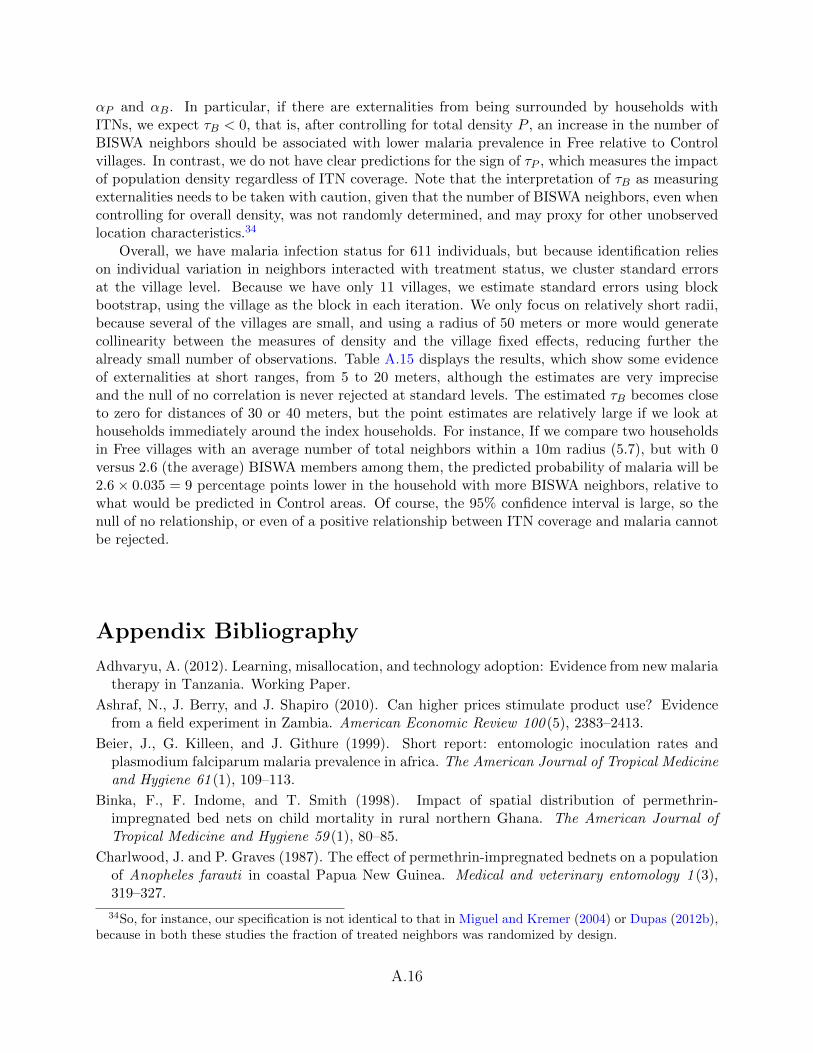
The villages included in our sample were selected from a list of 878 villages where BISWA operatedin 2007. These villages were spread across 318 panchayats (administrative unions of villages) in26 blocks across the five districts of Bargarh, Balangir, Keonjhar, Khandhamal and Sambalpur(see Figure A.1). We selected 150 villages for the study, stratified as follows: 33 from Balangir,48 from Bargarh, 30 from Keonjhar, 9 from Khandhamal and 30 from Sambalpur (the allocationwas approximately proportional to the number of BISWA communities in each district). Villageswere drawn using a pseudo-random number generator, with a selection algorithm that ensured theinclusion of a multiple of three villages from each block. Blocks where the Government of Orissawas planning to initiate free distribution of nets were excluded from the sampling frame. Whilethe study locations were thus chosen to minimize this risk, the sampling scheme was designed topreserve the balanced structure of the sample across treatment groups in case the state Governmentinitiated any unanticipated distribution. Data collected during the post-intervention survey showthat indeed distribution of nets from the Government (or from other NGOs) was extremely limitedin study areas, see Tables 2 and A.12. After the baseline survey, but before the intervention, nineof the 150 villages were found to have no actual BISWA activity and were then excluded from thestudy. Data from these villages are excluded from the analysis.
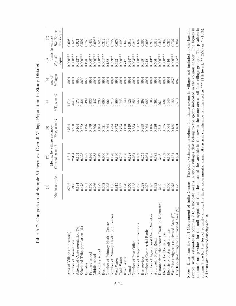
In Table A.7, we evaluate the characteristics of communities in our sample relative to othercommunities in the five study districts, by using data from the 2001 Census of India on a broadrange of village-level characteristics. Overall, the five study districts included a population of 8,991villages. Although the data used in this paper have been collected from 2007 onwards, the timegap relative to the 2001 census is short enough that a comparison between sample and non-samplevillages should be informative.
The results show that the null hypothesis of equality of means between sample and non-samplevillages is strongly rejected for most village characteristics (column 6). Sample villages are relativelylarge (both in terms of area and population), with mean total population more than twice as largeas in non-sample villages. Sample villages also appear to be closer to towns, although not to alarge extent. Mean distance from the nearest town is 35 kilometers among non-sample villages and1-10 kilometers less in sample villages. Amenities are overall significantly better in sample villagesas reflected, for instance, in the higher proportion of villages with schools, health centers, a postoffice, a telephone connection and electricity. Interestingly, sample villages are also characterizedby significantly larger fractions of land devoted to rice cultivation. This may have implication onmalaria prevalence, because rice fields are often an ideal breeding ground for larvae of Anophelesmosquitoes.
A.1
We also test the null hypothesis that village characteristics are on average equal in the threeexperimental arms (column 7). This is useful, because the randomization tests in Table 1 onlyevaluated balance in household-level characteristics among villages included at baseline. In a listof 26 variables, the test of equality across groups is only rejected, at the 10% level, for the presenceof a middle school in the village.
A.2 Details of Blood Tests
The RDTs were conducted using fingerprick samples of less than 0.5 ml of blood for each test.Malaria prevalence was determined using the Binax Now malaria RDT. This test is well validatedin comparison to blood smears for the diagnosis of malaria. The RDT detects both current andrecent infections, up to 2-4 weeks prior to the test. The result of the RDT is read on a test strip,located on a card, where a reagent is added to the blood sample. Recent infection is detected whenthe presence of Plasmodium antigens in the blood (histidine-rich protein 2, or HRP2) is signaled bythe appearance of darker lines on the white strip. High concurrency between test readers (includingnon-trained ones) has been documented in clinical trials of the RDT (Khairnar et al. 2009). Thetest does not indicate the level of parasitemia, and only delivers a positive/negative result formalaria infection, besides showing whether that infection is due to P. falciparum, to one of theother Plasmodium species, or to both (Moody 2002, Farcas et al. 2003, van den Broek et al. 2006,Khairnar et al. 2009). The test has been shown to have both good specificity and sensitivity. Boththese concepts are defined assuming that the “null hypothesis” of the test is that the individual doesnot have malaria. The specificity is calculated as the fraction of negative cases correctly diagnosedas such (that is, it is equal to one minus the probability of a Type-I error). The sensitivity is thefraction of positive cases correctly diagnosed as such (that is, one minus the probability of a Type-IIerror).
Hemoglobin levels were tested with the HemoCue 201 Hb analyzer, a portable, accurate systemfor measuring Hb. The test, like the one used to detect malaria prevalence, requires less than 0.5ml of blood and delivered results in approximately 15 minutes.
A.3 Gender and Age variation in Malaria and Anemia Rates atBaseline
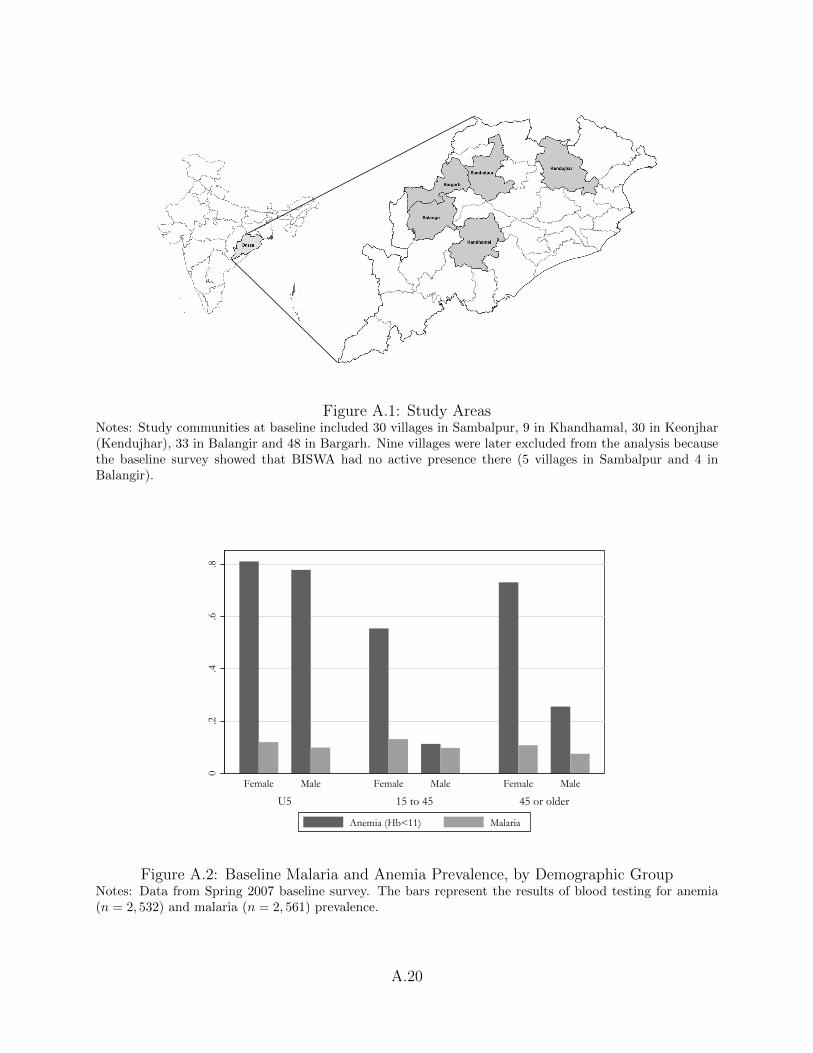
In Figure A.2 we show malaria and anemia prevalence by gender and age group. Women were 3 ppmore likely to test positive for the parasite, and the difference is significant at the 5% level. Thereis overall little variation in prevalence by age group, although when we disaggregate the data intosingle-year age bins we find that prevalence follows an inverted U-shape pattern with respect toage (results not shown).28 Such age patterns are commonly observed in malarious areas, becausevery young children have initially some immune protection from the mother (and are more oftenprotected by bednets, when available) although such immunity is gradually lost and subsequentlyreplaced by their own semi-immunity acquired through repeated exposure to the disease, so thatmalaria prevalence usually peaks for children of age 2-10 years (see Smith et al. 2007 for a reviewof the evidence). Sharma et al. (2006) found similar non-monotone age gradients in incidence andprevalence in Sundargarh, a district of Orissa that shares borders with two of our study districts.
There was substantial variation in anemia rates by gender and age. Approximately 80% oftested U5, of either gender, were anemic. Anemia rates declined significantly among adults aged15 to 45, but prevalence remained extremely high (60%) among women, while it was less than
28The same inverted U-shaped patterns was also found at follow-up, results not shown.
A.2
12% among men. Prevalence increased again among older adults, where it characterized aboutthree-quarters of women and one quarter of men. Similar patterns for anemia for different agesand genders are common in developing countries (see for instance Thomas et al. 2006), and arealso present in data from Orissa collected as part of the Indian National Family and Health Surveyin 2004-05, which showed an anemia prevalence of 65% among U5, 34% among women 15-49 andonly 8% among men in the same age group.
A.4 Details of Bednets and Treatment with Insecticide
The nets were of uniform quality, composed of white polyester multifilament, mesh size 156, and 75denier. They had a bottom reinforcement of 28 cm, with single nets measuring 180×150×100 cmand double nets measuring 180×150×160 cm. A total of 6,750 single and 3,250 double nets weresupplied by Biotech International Limited, who generously donated 5,000 single and 2,500 doublenets.
The bednets were treated on the spot at the time of delivery by trained personnel, follow-ing rules recommended in World Health Organization 2002, using K-Othrine flow, which containsdeltamethrin, a highly effective pyrethroid. The subsequent re-treatments after six and 12 monthswere done similarly by our trained collaborators, using the same guidelines. While wearing gloves,the field worker dipped the washed net into a bucket where water had been mixed with the appro-priate quantity of insecticide. After being soaked for a few minutes, the net was removed from thebucket and was laid flat on a plastic sheet or mat in the shade to dry. The concentration of theinsecticide was determined based on the manufacturer’s instructions: 10 ml of insecticide to 500ml of water for single nets and 15 ml-750 ml for double nets. The chemical concentration madere-treatment optimal after six months.
The study design did not incorporate the systematic use of ‘bioassays’, that is, procedures totest rigorously the insecticidal power of treated bednets. However, at the conclusion of the study,samples from four ITNs gathered from Free villages were tested through gas chromatographicanalysis, and two of the nets still had concentrations of deltamethrin around the concentrationsrecommended by the WHO (15-25 mg/m2), while the other two bednets had lower concentrations.Although the number of ITNs tested is obviously very small, the results do not signal obviousshortcomings with the re-treatment operations, given that the bednets had been last re-treated 6-7months earlier, and that it is not unexpected to find low insecticide concentrations six months afterre-treatment (particularly if the ITN has been washed multiple times).
Pyrethroids have been widely used for bednet impregnation with encouraging evidence aboutthe lack of side-effects on human health (World Health Organization 2005). In Orissa, syntheticpyrethroids have been in use since 1999, and tests performed in 2002-03 in several districts (includingour study districts Balangir, Khandhamal and Keonjhar) showed high rates of susceptibility todeltamethrin of Anopheles culicifacies and A. fluviatilis, the two most common malaria vectors inthe state (Sharma et al. 2004). The insecticidal efficacy of deltamethrin compound has also beenconfirmed in Sundargarh, which borders the study district Sambalpur (Yadav et al. 2001, Sharmaet al. 2006).
A.5 Attrition
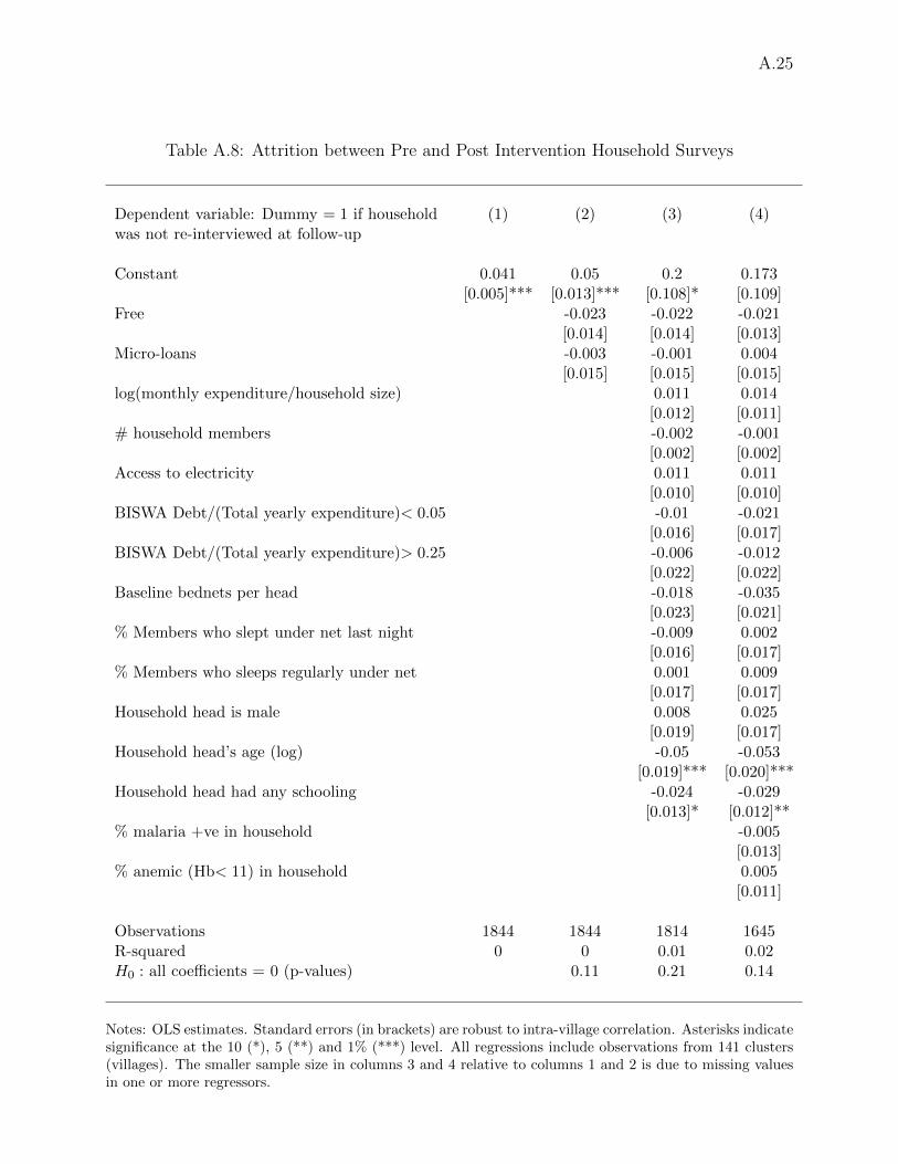
At follow-up, the survey team attempted to re-contact all households included in the baseline survey.The survey protocol called for at least three attempts, although a handful of households were re-contacted after 4 or 5 visits. Refusals accounted for only 13 of 76 lost households. As a result,attrition was limited, and of the 1,844 initial households, 1,768 (96%) were re-interviewed. Attrition
A.3
was 5% in MF and control villages and 3% in Free communities (see Table A.8, column 2). The nullof equal attrition rates among arms is not rejected at standard levels, regardless of whether we useindividual or joint tests. There was little correlation between attrition and household characteristicsat baseline, including RDT results and bednet ownership and usage (columns 3 and 4). The onlyregression coefficients that are individually statistically significant indicate that households withan older and better educated head were less likely to exit the panel. On the other hand, we cannotreject the joint null that all the included slopes are equal to zero (p-value=0.14).
We also investigated whether significant changes in household composition took place betweenthe baseline and the follow-up survey, as well as whether such changes were balanced across experi-mental arms. This was potentially important for two reasons. First, changes in availability of ITNsmay have arisen from changes in the number and age of households members (for instance, youngchildren often share a sleeping space with their parents). Second, malaria and anemia prevalence atbaseline differed across age and gender groups (see Figure A.2), so that changes in the demographicstructure of the household may have confounded aggregate changes in such health measures cal-culated over all household members. We looked at both entry into or exit from panel householdsand to changes in the relative weight of different demographic groups. This analysis was possiblebecause enumerators filled a complete household roster both at baseline and at follow-up, so thatwe can separately identify new members as well as individuals who left the household because ofdeath or relocation. We find that these factors did not plausibly drive any of the results in the pa-per. We omit the detailed analysis for brevity but the interested reader can find it in the appendixof Tarozzi et al. (2011).
A.6 The Information Campaign and Household Survey as PossibleConfounders
In principle, the relatively high ITN adoption rates observed with micro-loans may have been ex-plained at least in part by the information campaign (IC) and household survey cum RDTs thatpreceded the sales. These factors may have made the malaria problem more salient, leading to highdemand regardless of the possibility to pay over time rather than in cash. There is indeed growingawareness within field-based development economics that surveys may themselves constitute ‘in-terventions’, see e.g. Zwane et al. (2011). In this section we argue that although such confounderslikely played a role, they cannot plausibly explain more than a fraction of the high demand observedwith micro-loans.
As a first point, we note that confounders were also present in the recent seminal studies thatdocumented very steep demand curves among poor populations in developing countries. ITN salesin Cohen and Dupas (2010) took place at ante-natal visits, during which the importance of ITNswas discussed and hemoglobin levels were measured (p. 14). In Ashraf et al. (2010), the baselinesurvey also included a number of questions on water use practices and Clorin adoption, as wellas measurements of the concentration of chlorine in households’ drinking water supply (pp. 2389-2391). In this experiment, the water disinfectant Clorin was sold during door-to-door marketingvisits. The de-worming project studied in Kremer and Miguel (2007) was carried out with teachertraining, teacher and NGO-led school lessons, and a number of classroom educational materials(pp 1013-1015). In addition, in that study the huge drop in demand for drugs observed after theintroduction of cost-sharing was also observed in areas where pupils had been tested for intestinalworms infections and had been part of the de-worming campaign. From this perspective, our studydesign was comparable to that of these earlier studies and we show that, if anything, it couldperhaps be singled out for its unusual ability to study the impact of such behavioral components.
A.4
A.6.1 The IC as a possible confounder
We first discuss the IC, which we argue was not a plausible key confounder. First, the IC wasa simple one-time presentation about malaria, the means by which it is transmitted and the im-portance and rationale for ITN use, a demonstration of how to hang nets properly, and adviceon proper use and re-treatment. Such presentation usually lasted less than one hour, and a largemajority of households were already familiar with the IC content, with the major exception of theimportance of treating bednets regularly. For instance, at the time of the baseline survey, 96% ofrespondents stated (un-prompted) that malaria was transmitted by mosquitoes, while 95% statedthat bednets can prevent the disease (although less than 3% explicitly mentioned ‘ITNs’ ratherthan ‘bednets’). Second, the IC conducted before the sales on credit in 2007 and the one before thecash sales in 2011 were very similar, and yet the resulting demand was significantly different. Third,we demonstrated that in control areas there was virtually no change in ITN usage between baselineand follow-up (Table 2, column 5). During the same period there was only a small increase (0.3bednets per households) in the number of bednets owned, suggesting that the IC did not changebehavior or perceptions of malaria risk substantively. Fourth, additional evidence comes from ahousehold survey conducted at the same time as the follow-up survey—in Winter of 2008-09—in25 villages that had not been part of the initial study.
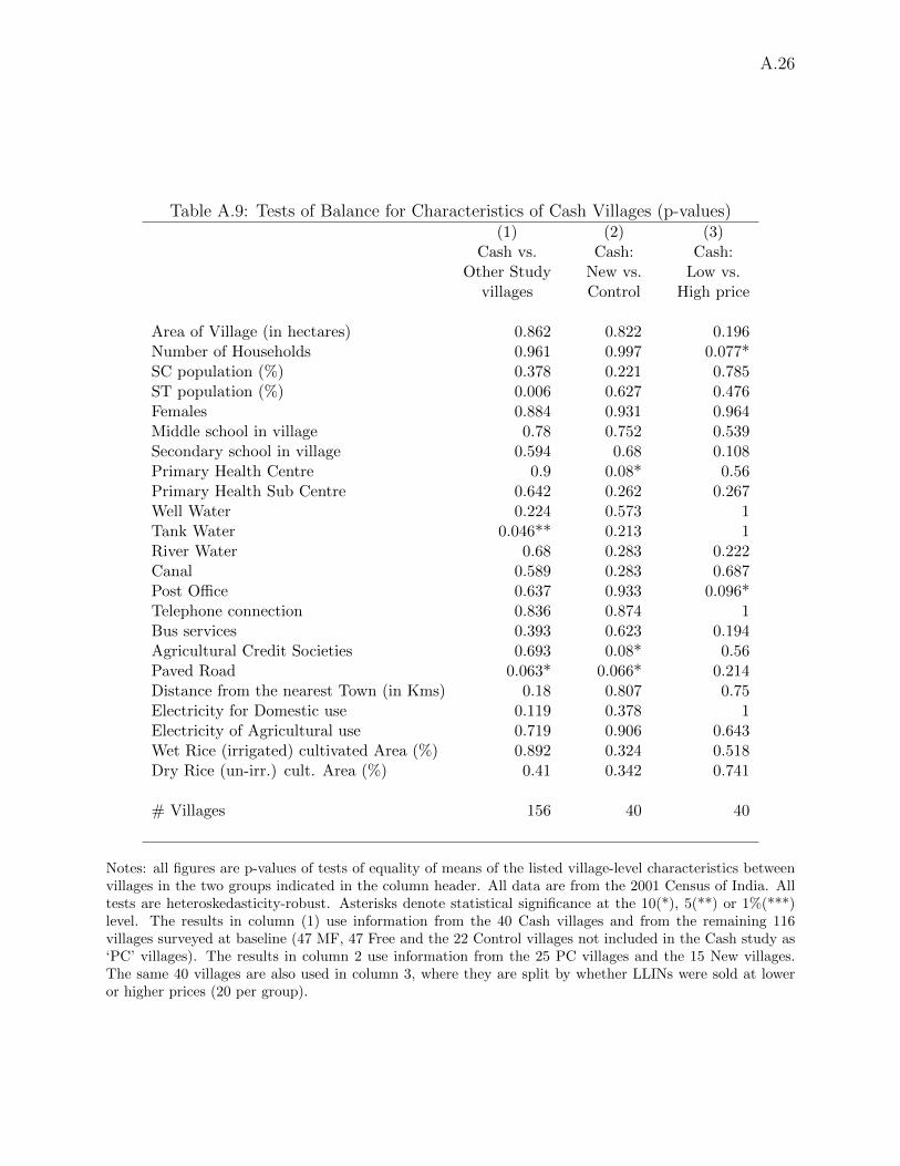
These 25 villages were added specifically to allow for the separate identification of any impact ofthe IC and/or of the survey itself on behavior. These 25 ‘follow-up only’ villages (‘FUO’ hereafter)were selected from the same randomly sorted lists used for the selection of the communities atbaseline. In other words, we did not complete a new randomization, but we selected the “next25 villages” from the same randomization done in 2007. The similarity of the new village relativeto those included since baseline was confirmed by comparing the village characteristics includedin Table A.7 (measured during the 2001 Census) between the 25 FUO villages and the 141 studyvillages where the baseline survey had been conducted. The null of equality is rejected for onlythree of the 26 characteristics (results available upon request). In each FUO village, 15 householdswere selected regardless of BISWA affiliation, using simple random sampling from publicly availablecensus lists formed in 2002 as part of the ‘Below Poverty Line census’ by the Government of Orissa.Because BISWA had a strong presence in the study areas, the sample ended up including BISWAhouseholds in almost all villages (21/25).
When we compare sample households in Control areas to BISWA households in FUO villages,we find that the number of bednets was very close between the two groups, and the null of equalitycannot be rejected at standard levels: the mean was 0.36 per person in Control and 0.32 in FUO,and the p-value for the test of equality is 0.3248. Consistent with this result, the survey-elicitedsubjective probability of someone falling ill with malaria within a year when always sleeping underan ITN was 0.16 in both sub-samples.29 Overall, then, the data do not support the hypothesis thatthe IC affected behavior or perceptions about malaria substantively.
A.6.2 The baseline survey and RDTs as possible confounders
The baseline survey included a long list of questions about malaria and bednets. In addition, theresults of the RDTs were available on the spot, a few minutes after the blood sample was taken,and individuals were immediately informed about the outcome of the test. These factors may havemade the disease more salient, possibly increasing the willingness to pay for ITNs regardless of the
29These subjective probabilities were elicited by asking respondents to place a number of marbles rangingfrom 0 to 10 into a cup, with the number increasing in the probability of the event taking place in the future.Similar methodologies have been adopted in several studies, see Delavande et al. (2010) for a review.
A.5
possibility being offered to delay payment. Indeed we have shown that demand was significantlyhigher among households where at least one member tested positive to the blood test. We argue,however, that these factors cannot plausibly explain more than a fraction of relatively high demandfor ITNs on credit when compared with earlier studies that found very little demand for health-protecting technologies when these were not offered for free.
First, we have discussed before how comparable confounders (including health tests) were alsopresent in earlier studies that found very low demand for health products. In principle, suchconfounders may have been more important in our empirical context, but it is not clear why thisshould be the case.
Second, we have shown that, by comparing outcomes in Control areas with those of BISWAhouseholds in FUO villages, we found no evidence that the joint impact of the IC, the baselinesurvey and RDTs increased bednet ownership or changed perceptions about the effectiveness ofITNs. Even so, we cannot rule out the possibility that demand would have been higher in the Newvillages in the Cash arm if we had filled the same questionnaire and conducted the same RDTs inthese communities (these elements could not be added to the supplemental arm due to time andfunding constraints). In PC villages, however, both potential confounders had been present, albeitmore than four years prior to the Cash intervention. As we pointed out earlier, there is no differencein ITN adoption between PC and New villages which at least suggests that the surveys and RDTshad no longer term effects on take-up. In addition, within PC villages, demand is very similar (andlow) when we directly compare households who had been exposed to the survey and RDTs, andothers who had not (see rows F and G of Table 4). Recall also that attrition between baseline andfollow-up was very limited, so almost all sample households in PC villages had been exposed to alengthy questionnaire and RDTs both at baseline, in 2007, and at follow-up, in 2008-09.
To probe this issue further, we can use data about ITN purchases in MF villages among BISWAhouseholds not included in the pre-intervention survey, among whom biomarkers were not collected.At the time of the MF sales, in 2007, surveyors recorded the number and type of ITNs purchased byall BISWA members, regardless of their inclusion in our sample. Our data do not include the totalnumber of ‘BISWA households’ in study villages, but this number can be estimated from the listsof BISWA members supplied by the micro-lender at the beginning of the study. The latter figure isnot the correct one to be used for the estimation of demand among non-sample households, for tworeasons. First, some households had more than one member affiliated to BISWA (on average 1.11).Second, a fraction of individuals listed as BISWA members were found not to be such during thefield work, or had migrated, or were otherwise excluded from the study population. In this way, weestimate that every 100 members listed by BISWA corresponded to about 79 BISWA households.Let n and ns denote respectively the total number of buyers in MF villages and the number of buyersamong sample households. Let also m denote the initial number of BISWA members provided bythe micro-lender, and let ms denote the number of baseline sample households in the same villages.We thus calculate demand among non-sample BISWA households as (n−ns)/(0.79m−ms) = 0.28.Uptake was then about twice as large as that observed among BISWA members who were offeredLLINs for cash at the same nominal price (.149, see Table 4), and about four times as large as thatobserved when the price was kept constant in real terms (.073). In addition, as described earlier,these figures likely attenuate the differences in demand between Cash and MF, because the vouchersystem implies that a BISWA member who was not present during the voucher distribution wouldnot be counted in the demand estimation, rather than being counted as not having purchased.
Another key factor points to the fact that the 28% take up rate among ‘non-sample’ BISWAhouseholds in MF communities is artificially biased downwards relative to demand among samplehouseholds. That is, field reports indicate that more effort was put into ensuring attendance of
A.6
sales meetings for sample relative to non-sample households. In fact, during the first sale session,78% of baseline households attended the sale, while only 56% did among non-baseline households.Similarly, during the second session, conducted 1-2 weeks afterwards, attendance rates were 62and 40% for the former and latter group respectively. Of course, attendance itself may have beeninfluenced by the inclusion in the baseline.
To summarize: we argue that while the IC and the baseline surveys may have played a role inincreasing take-up, the effects are not sufficient to explain the overall take-up rates.
A.7 Respondent-reported Malaria Incidence versus RDT Results
As we mention in Section 4, our data on malaria incidence are derived from respondent reportsand not from blood tests. Such reports may be noisy indicators of actual incidence and may alsosuffer from bias potentially differential across experimental arms. For instance, the distribution ofITNs may have made the disease more salient, pushing respondents to over-report illnesses or itmay have led to a decrease in the perceived malaria risk, with opposite effects on program impacts.In this section we provide evidence in support of the view that, despite these concerns, incidencedata in our data set were a valuable source of information on malaria burden.
First, note that reported incidence can be validated against the RDTs only for very recentmalaria episodes, because the RDTs we used in the field can only detect malaria episodes thatare still ongoing or that took place no more than 2-4 weeks earlier (see Appendix A.2). Let thebinary variable Si = 1 if individual i was reported as having had malaria in the month precedingthe survey, and let Mi = 1 if the individual tested positive for malaria when tested with a RDT.In our post-intervention sample, there is a total of 63 individuals for whom Si = 1 and for whomwe observe Mi. Among these 63 individuals, 28 (44%, 95% C.I. 0.32-0.57) also have Mi = 1. Aswe discuss in the paper, most malaria cases detected by the RDTs were apparently asymptomaticand thus not mentioned by respondents, but despite this the self-reported information about recentmalaria incidence is strongly correlated with the RDTs. To show this we estimate with OLS thefollowing model, using all individuals for which Mi and Si are non-missing
Si = β0 + βMMi + ui.
The estimated intercept is β0 = 0.006 while βM = 0.012 and is significant at the 1% level (p-value= 0.006, adjusted for clustering at the village level, n = 7, 153). In other words, self-reportedrecent incidence was three times as large for individuals who tested positive relative to others whodid not.
That respondents were able to recognize symptomatic malaria episodes is also confirmed by thefact that the results are very different if we estimate a regression such as the one above using asdependent variable a dummy = 1 if the individual was only reported as having had ‘fever’ duringthe last month. In this case, the intercept is 0.03 while βM = 0.002 and is not significant at anystandard level (p-value= 0.715, adjusted for clustering at the village level, n = 7, 153).
Another key observation is that the link between Si and Mi does not appear to be differentialacross experimental arms, so there is no compelling evidence that the intervention changed per-ceptions about malaria incidence conditional on actual malaria infection. The fractions P (Mi =1 | Si = 1) are 42% in Control areas (8/19), 45% in Free (10/22) and 45% in MF (10/22). Thefractions are thus almost identical, and the null of equality cannot be rejected (p-value= 0.9724 forthe joint null of equality. The individual differences are also not significant).
A.7
A.8 Post-intervention RDT Success Rates
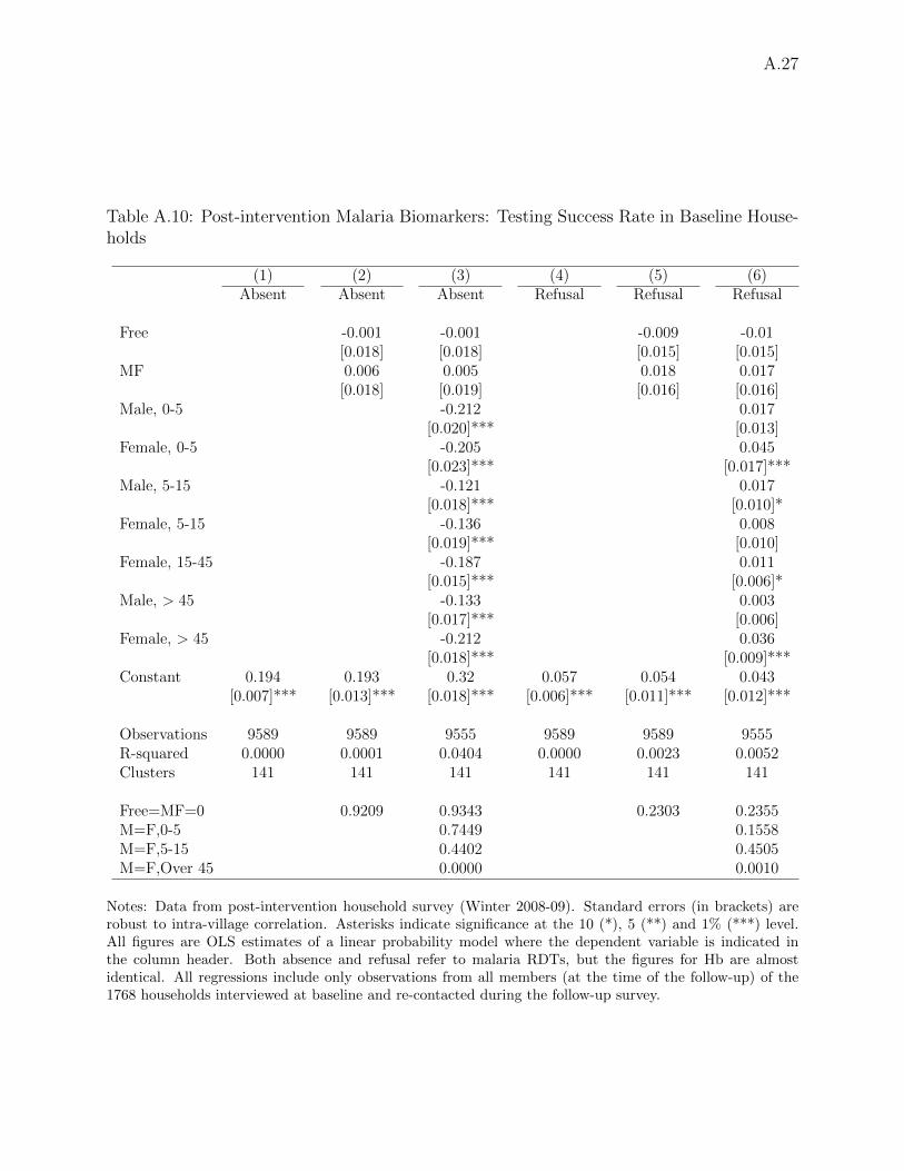
In the post-intervention survey, all members of households re-contacted after the baseline weretargeted for blood tests. Our testers were able to successfully test 75% of members in panelhouseholds, while 19% could not be tested because they were not present at the time of the visitsand only 6% because consent was not given, see columns 1 and 4 in Table A.10. The figures incolumns 2 and 5 show that absence and refusal were almost identical across experimental arms.Conversely, we find differences in testing success across different age groups (columns 3 and 6).Almost one third of adult males (15-45, the omitted category in the regressions) could not betested because of absence during the visits, probably because they were more likely to be offto work. Testing rates among all other demographic groups were substantively and statisticallysignificantly higher, especially among U5 of either gender and among women 15 years old andabove. For these groups, testing rates were close to 90%. The testing rates are very close betweenboys and girls, and the null of equality between genders cannot be rejected for both U5s and 5 to15 year old children. Refusal rates were highest among women over 45 (8%) and girls U5 (9%).Refusal rates were 3 pp lower among U5 boys relative to girls but the null of equality betweengenders cannot be rejected at standard significance levels.
A.9 Changes in Malaria Indices by Demographic Group
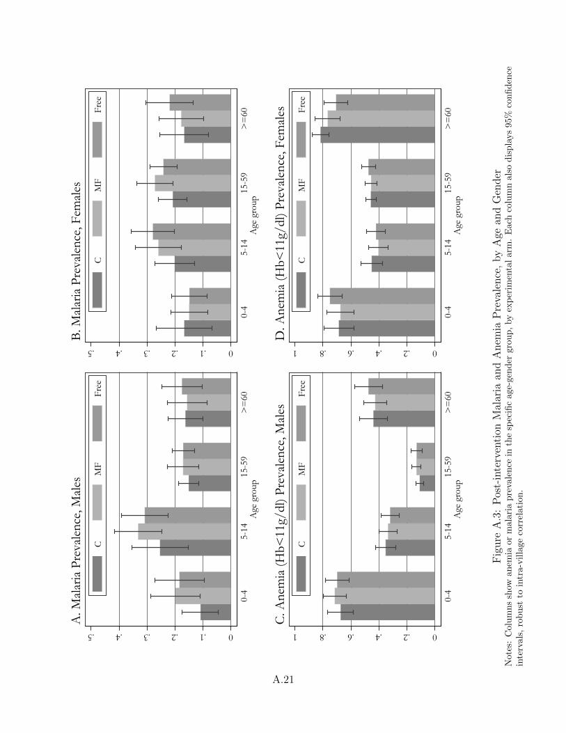
Was the lack of health benefits shared by all demographic groups? The bars in Figure A.3 showmalaria and anemia prevalence for each experimental arm by gender and age group, together with95% confidence intervals.
Among adult males (age 15 or above), malaria prevalence was ∼15% and almost identical acrossarms (panel A). Among U5s, prevalence was 11% in control villages but about twice as large inintervention communities: 18.4% in Free and 19.8% in MF villages. However, the estimates areimprecise, and the difference relative to control is not significant at standard levels, although thep-values are relatively small (below 0.2). Details of the test statistics are available upon requestfrom the authors. Prevalence among males is highest among 5-14 boys, where in each arm it is ∼15pp higher than for younger children, so that the differences among groups are almost identical inthese two age groups.
These patterns change when we look at females (panel B), although again differences betweenarms are never significant at standard levels. Among females, we observe almost identical prevalenceacross arms among the youngest girls (∼15%) and higher prevalence in intervention villages in olderage groups. In each experimental arm, the highest prevalence is observed among females of age 5to 59.
Overall, these results document remarkable differences in malaria prevalence across sub-groups,but these differences are largely concentrated between genders or across age groups rather thanacross experimental arms. Note also that, consistent with the baseline results, we do not observeprevalence rates monotonically declining with age. The relatively low prevalence among U5s isactually driven by very low rates among children less than two years old (results not in the figure).Of a total of 263 children in this latter age group, only 12 (4.6%) tested positive, while prevalencejumps to 23.3% among the 412 two to four years old tested. Overall, in our sample malariaprevalence peaks among 5 to 10 years old, and then gradually declines with age. These patternsare similar among experimental arms.
Consistent with the baseline results, the results for anemia (panels C and D) show large sys-tematic gaps across gender-age groups. In particular, these results confirm the U-shape of anemiaprevalence with respect to age for both genders, as well as the significantly higher anemia rates
A.8
among females 5 and older relative to males of the same age. Like for malaria, however, thedifferences in anemia prevalence between arms are small and never significant at standard levels.
A.10 RDT Validation Study
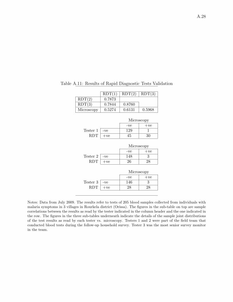
In July 2009, we carried out a small validation study after the conclusion of the follow-up survey incollaboration with the Malaria Research Centre (MRC) Field Station in Rourkela (Orissa), whichconfirmed the accuracy of the RDTs. A total of 205 blood samples were independently collectedfrom the MRC team from individuals with malaria symptoms from three villages. The RDT cardswere interpreted by three different blinded readers, including two of the testers who were part ofthe field team during our study, and the most senior survey monitor in our research team. Theseresults were then compared with thick and thin blood smears read with microscopy by the MRCteam for the same samples, with the smear result accepted as the correct infection status. Theresults showed very high sensitivity (> 90% for each of the three readers, see Table A.11 for details).The fraction of correctly identified negatives (specificity) ranged from 74 to 85%.
The lower specificity (higher prevalence) measured by the RDTs relative to microscopy was notsurprising, given that these tests may detect the presence of the P. falciparum antigens up to 2-4weeks after parasitemia has cleared (Humar et al. 1997). The RDT results were overall very similarbut not identical between readers (pairwise correlations ranged from 0.78 to 0.88). In columns 9and 10 of Table 5, we show that the ITT estimates for malaria prevalence remain almost identicalif we include tester fixed effects in the regressions.
A.11 Changes in Other Prophylactic Behavior
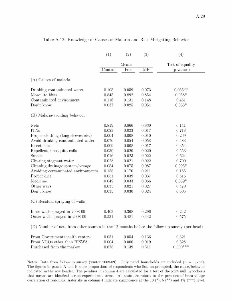
In Table A.12, we look at differences among experimental arms in knowledge about causes ofmalaria (panel A), precautions one can take against it (panel B) and wall spraying between base-line and follow-up (panel C). The survey instrument asked respondents—without prompting—tolist all possible causes of malaria, and then asked “[w]hat are the best precautions you can taketo protect yourself from getting malaria.” In each arm, 85% or more of respondents list mosquitobites as a cause of malaria. Overall, households in intervention communities appear to be about asknowledgeable regarding causes of malaria as those in control areas, although the test of equalityis rejected at the 10% level (but not at the 5%) for three of the four causes of malaria, and in eachof these cases it is one of the experimental arms that suggests the best knowledge. There was nosystematic variation in malaria-avoiding behavior among groups (panel B). Bednets are by far themost commonly listed precaution, mentioned by 82-87% of respondents (with the highest propor-tions in intervention villages). The next two most common precautions are “avoid contaminatedenvironment” (16-21%) and “avoid drinking contaminated water” (5-8%). For all the fourteen in-dices, the test of equal means is not rejected at the 5% level, although the null is rejected at the10% in two cases, and the joint null of equality for all behaviors is rejected (p-value = 0.0421).However, the differences are not consistent with risk-averting behavior being more common in con-trol villages, and indeed in several cases they indicate the opposite (for example, use of smoke orlong sleeves, or cleaning of drainage pools).
In panel C we analyze differences in residual spraying of indoors or outdoor walls. Althoughthe null hypothesis of equal proportion among treatment groups cannot be rejected at standardlevels, the magnitude of the differences between control and intervention areas is large. The reasonwhy the null is not rejected despite the large differences is that the intra-village correlation forthese two variables is very large (0.41 and 0.63 for inner and outer spraying respectively). Our datado not tell us if these differences were driven by household decisions, or if instead they resulted
A.9
from choices made by public health officials who may have scheduled wall spraying taking intoaccount our intervention. To evaluate whether differences in spraying rates help explain the lackof health benefits in intervention villages, we re-estimate the ITT model for malaria prevalenceincluding dummies for recent wall spraying among the regressors, but this leaves the estimatedimpacts almost identical (see columns 9 and 10 of Table 5).
A.12 Changes in Local Anopheles Behavior or Resistance to In-secticide
In principle, changes in the characteristics of the local Anopheles population may explain the lackof improvements in malaria and anemia prevalence. First, Anopheles mosquitoes may have beenresistant to deltamethrin, the insecticide used to impregnate study bednets, or they may havedeveloped resistance during the course of the study. Second, the reduction in malaria transmissionmay have been hampered if local Anopheles took a sufficiently high fraction of blood meals outsideof the sleeping hours, when individuals were less likely to be protected by ITNs. In principle, alarge increase in the fraction of individuals protected by bednets, as well as the excito-repellentproperty of deltamethrin, could lead to changes in peak biting hours, or in indoors vs. outdoorsfeeding habits. The increased difficulty in finding blood meals during the sleeping hours could forcemosquitoes to increase biting at times when individuals are not protected by ITNs. Our projectdid not collect information on the local Anopheles population, before or after the intervention, sowe cannot address these concerns directly. However, a number of factors make these hypothesesunlikely to hold.
First, recent studies carried out in Orissa suggest that local Anopheles biting patterns andsusceptibility to deltamethrin made ITNs a promising protective tool against malaria. In Keon-jhar, one of our study districts, Sahu et al. (2009) found that biting activity of the main localmalaria vectors was concentrated between 2100 and 0300 hours, regardless of the season. Sharmaet al. (2004) describes tests performed in 2002-03 in several Orissa districts (including our studydistricts Balangir, Khandhamal and Keonjhar). The tests showed high rates of susceptibility todeltamethrin of Anopheles culicifacies and A. fluviatilis, the two most common malaria vectors inthe state. The insecticidal efficacy of deltamethrin compound has also been confirmed in Sundar-garh, which borders the study district Sambalpur (Yadav et al. 2001, Sharma et al. 2006). Thefield work for these studies was conducted a few years before our project, but a very recent studyin Sundargarh, conducted in 2009-2010, found that synthetic pyrethroids were still highly effectiveagainst both A culicifacies and A fluviatilis, despite the fact that study areas had been exposedto either large-scale spraying with pyrethroids or to large-scale free distribution of bednets treatedwith deltamethrin, the same synthetic pyrethroid adopted in our study (Sharma et al. 2012). An-other recent study, carried out in 2009 in Madhya Pradesh, central India, found some evidenceof resistance to deltamethrin, but even in areas that had been sprayed regularly in the previous5-10 years, the researchers documented about 75% mortality rates in the local population of Aculicifacies when exposed to the chemical (Mishra et al. 2012).
Second, although the emergence of resistance to insecticides such as DDT and pyrethroids hasbeen documented following widespread use in agriculture or wall spraying, there is as yet littleevidence of resistance developing as a consequence of the introduction of ITNs. Even in situationswhere resistance is present, ITNs have been documented to retain some protective efficacy (Enayatiand Hemingway 2010). The only exception we are aware of is Trape et al. 2011. In this study,the authors found that the introduction of deltamethrin-treated LLINs in one village in Senegalled initially to sharp reductions in malaria incidence and prevalence, but that resistance to the
A.10
insecticide became widespread in about two years. This led to an increase in malaria morbidityrelative to before LLINs distribution among adults and older children. However, unlike in ourstudy, nets were distributed to all villagers, and ownership and usage rates remained around 60-80% throughout the study period (and were close to 100% at the onset of the study).
Third, the literature is overall inconclusive about the impact of ITNs on Anopheles biting pat-terns, with only a fraction of the evidence pointing to changes in mosquito behavior that mayhave reduced the efficacy of nets (Takken 2002, Pates and Curtis 2005). After the distribution ofpermethrin-treated bednets to all inhabitants of one hamlet in Papua New Guinea, Charlwood andGraves (1987) observed a relative increase in biting during the evening, although the number ofAnopheles in the area decreased substantially. Similar results were also found after mass distribu-tion of ITNs in five villages in Tanzania (Magesa et al. 1991) and in locations where ITNs weredistributed to cover all beds in Kenya (Mbogo et al. 1996) and Benin (Moiroux et al. 2012). Notethat in all these studies ITNs had been delivered to ensure universal coverage, a situation in starkcontrast with our case.
In sum, the existing evidence points to the likely efficacy of deltamethrin-treated ITNs in ourstudy areas, and the literature suggests that the relatively low coverage of ITNs at the communitylevel would have been unlikely to produce the emergence of either insecticide resistance or changesin biting patterns that may have reduced the benefits of the intervention.
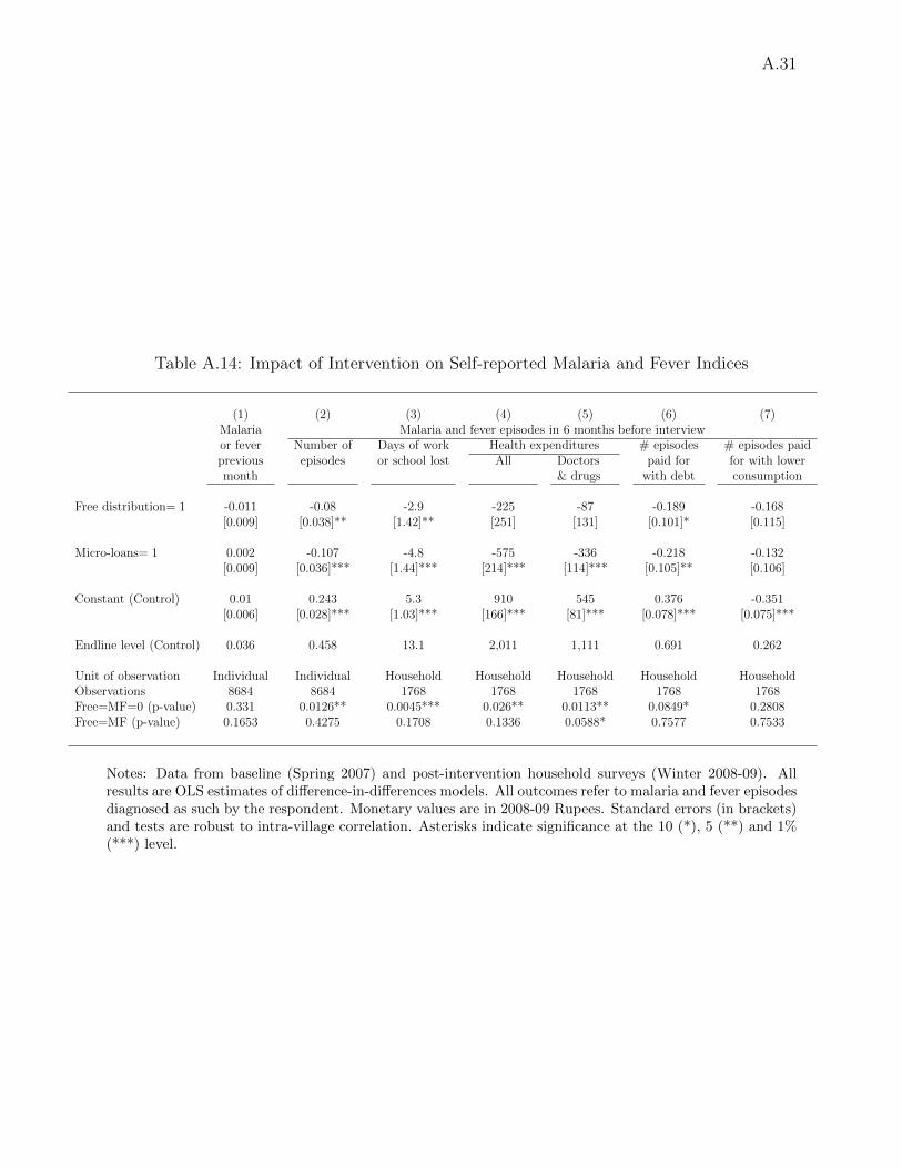
A.13 Impacts on Self-reported Incidence Adjusted for Misdiag-noses
In Appendix A.7 we have shown that only 44% of the individuals reported as having had malariain the same month as the interview tested positive to malaria. Some of these individuals may haverecovered from malaria by the time blood samples were taken, but it is likely that the discrepancyis at least partly explained by misdiagnoses. In malarious areas, while asymptomatic cases arecommon, it is also common to attribute to malaria other fever episodes not caused by this disease(see for instance Adhvaryu 2012, Cohen et al. 2012). In such case, the figures in column 2 ofTable 6 could confound changes in symptomatic malaria cases with changes in other symptomaticfever episodes. In addition, our data show that respondents were also misdiagnosing some malariaepisodes as ‘fever’. This can be seen looking at the RDT results among individuals reported ashaving had fever during the same month as the interview. Among these 221 individuals, we findthat 22% tested positive to malaria (95% C.I. 0.16-0.29).
In this section we use these considerations to construct a procedure to adjust the impacts onincidence in column 2 of Table 6 in a way that takes misdiagnosis into account. Note that weare not interested in estimating the program impacts on ‘true’ malaria incidence (regardless ofwhether an episode was recognized by the respondent), but rather we aim at estimating impactson symptomatic malaria incidence. We argue in the paper that the latter is of interest because itmeasures cases severe enough to be perceived and to lead to illness-related costs recognized by therespondent. Recall that our data include both self-reported malaria cases and self-reported fevercases. Suppose that MA,ti represents the number of malaria cases during the previous six monthsreported for individual i from experimental arm A (A = Free,MF,Control) interviewed at time t(where t = 0 denotes baseline and t = 1 denotes follow-up), while FA,ti is the corresponding figurefor self-reported fever incidence. We assume that errors of diagnoses for symptomatic cases happenat the same rate over time and across different experimental arms (see Appendix A.7 for someevidence in support of this assumption). Consistent with the estimates above, we then assume thatonly 44% of self-reported malaria cases are actually malaria, but also that 22% of self-reported fever
A.11
cases were actually malaria. We can thus estimate the mean number of actual malaria episodes attime t in a given treatment arm as 0.44× MA,t + 0.22× FA,t, where MA,t and FA,t are respectivelymalaria and fever incidence as measured in our raw recall data.
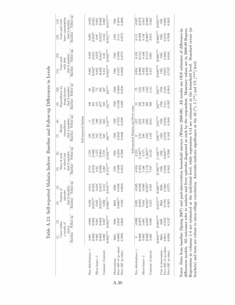
Next, let βDDY,T denote the estimated difference-in-difference impact on outcome Y = M,Ffor treatment T = MF,Free versus control areas. From column 2 of Table 6 we estimate thatβDDM,Free = −0.048 and βDDM,MF = −0.051. Similarly, when we estimate the same model using F
as dependent variable we obtain (results not shown in the table) βDDF,Free = −0.032 (s.e. 0.033, so
not significant) and βDDF,MF = −0.056 (s.e. 0.031, significant at the 10% level). Because the DD isa linear combination of time and arm-specific means, and under the previously stated assumptionthat mid-diagnosis errors of symptomatic illness are non-differential across arms and over time, theadjusted DD for actual symptomatic malaria incidence can be finally calculated as 0.44× βDDM,T +
0.22× βDDF,T , T = MF,Free. The final estimates are thus −0.048× 0.44− 0.032× 0.22 = −0.028
(s.e. 0.012) in Free and −0.051 × 0.44 − 0.056 × 0.22 = −0.035 (s.e. 0.011) in MF areas.30 Suchestimates are thus about 60% as large as those in column 2 of Table 6, although both remainsignificant and substantive in magnitude.
A.14 Epidemiological Models of ITN Use
Current advances in epidemiological models of malaria transmission may help explaining the linkbetween ITN usage and coverage and changes in malaria indices in our study areas. In particular,Killeen et al. (2007) describe a complex model that describes how malaria infection is affected byseveral factors, including mosquito numbers, biting patterns and mortality (also in relation to ITNpresence) and above all ITN coverage and usage. The model simulates the protective power of ITNsfor both users and non-users, by calibrating 16 exogenously determined factors (largely borrowedfrom earlier studies), and then showing how ITN protection varies with changes in coverage andusage. The protective power of bednets is measured as a relative risk (RR) of entomologicalinoculation rates (EIR), that is, the number of infective bites per year calculated relative to asituation where no ones uses nets. A useful feature of this study is that the authors also providea spreadsheet that can be used to analyze how changes in any of the exogenous factors affect theRR. The spreadsheet is available at http://www.ncbi.nlm.nih.gov/pmc/articles/PMC1904465/bin/pmed.0040229.sd001.xls.
Panel A in Figure A.4 shows one of the key results in Killeen et al. (2007): in a scenario whereabout 60% of the population always uses ITN, individuals without an ITN (the dashed line) areas protected as an individual who sleep regularly under an ITN in a community where no one elsedoes (the continuous line). A key assumption to produce these results is that the index individualusing the net does so very regularly. Specifically, panel A (identical to one of the graphs in Figure3 of Killeen et al. 2007) is produced assuming that the individual uses the net for 90% of thepotential time of exposure. In our empirical context, we have argued that information on previousnight usage of ITNs is reliable, but even so our data indicate that only 45% of the program ITNswere in use the night before the follow-up survey in Free villages, and about 30% were in use inMF communities. If we assume that the frequency of usage is equal to such cross-sectional usagerates, while leaving all other parameters in the epidemiological model unchanged, the associationbetween relative transmission intensity and coverage for users becomes as described in panel B ofFigure A.4. Even under such scenario ITNs would provide some protection, but if less than 20%
30To take into account that both 0.22 and 0.44 were estimated, we calculate the standard errors using1,000 block bootstrap replications, using the village as the block.
of the village population always uses ITNs (as surely is the case in a large majority of our studyareas), then the RR remains close to 0.6-0.7.
These results formalize the intuition that sleeping under an ITN, even when done irregularly,should be expected to decrease the number of infectious bites to some extent. However, whether thedecline is sufficient to produce a decline in malaria prevalence (our key biomarker) is not obvious.The link between EIR and prevalence is studied in Beier et al. 1999, who analyze data from 31studies throughout Africa where both outcomes could be estimated. They find that, after excludingtwo clear outliers the data are tightly concentrated around a linear regression relationship betweenmalaria prevalence and the logarithm of annual EIR (R2 = 0.712). Malaria prevalence predictedby the linear fit is 24.68 + 24.2 log10EIR, with the standard errors of intercept and slope equalrespectively to 3.06 and 5.42.
Although there is no direct information from Indian locations, the authors point out that“[w]hile malaria stratification according to ecologic zones is an important element of malaria control,it is important to note that the fundamental relationships between EIR and the prevalence of P.falciparum infection will likely hold across diverse ecosystems in Africa.” Together with the verytight distribution of the scatterplot around the regression line linking EIR to prevalence (see theirFigure 2), this suggests that a similar relationship will also likely hold outside of the Africancontinent. In areas neighboring our study districts, Sharma et al. (2006) documented EIR inthe range of 3-114 infective bites per year, depending on location, well inside the relevant rangeconsidered in Beier et al. 1999.
In our study areas, prevalence rates was about 20%, with village-specific prevalence rangingfrom 0 to about 60% and 95% of the 141 study villages showing prevalence below 0.53. Looking atFigure 2 of Beier et al. (1999), this suggests that the EIR in the area was likely between 1 and 10,but it also suggests that a 30-40% decline in EIR may have barely affected prevalence, given thatEIR in the 1 to 10 range are associated with a very wide spectrum of prevalence rates. Using thewords in Beier et al. (1999), “it may not be possible to achieve dramatic decreases in prevalence ofP. falciparum infection at sites in Africa unless control measures reduce EIRs to levels well below1 infective bites per year” (p. 111). Our results suggest that similar arguments will hold in othermalaria-endemic areas outside of the African continent, such as our study areas in Orissa.
A.15 Malaria Prevalence and ITN Coverage
Recall that only BISWA clients received free ITNs or the offer of ITNs for sale on credit. AlthoughBISWA has a large presence in the study area, we estimate that on average only 20% of peoplelived in households with at least one BISWA affiliate and thus were eligible for inclusion in thestudy.31 It is now accepted that the externalities offered by mass adoption of ITNs are a key factorfor ITN efficacy, although the relative role of personal versus mass protection of ITNs is not yet wellunderstood (Binka et al. 1998, Hawley et al. 2003, Killeen et al. 2007). Reductions in malaria indiceshave been documented among non-users of ITNs living within a few hundred meters of communitiescovered by mass distribution of ITNs. In our intervention, study villages were scattered spatiallyover a very broad geographical area (see Section 2), so cross-village externalities are not plausible.
31We estimated the fraction by making use of village population data from the 2001 census of India,together with estimates of the total number of individuals living in households with at least one BISWAmember. Let sv and bv denote respectively average household size and average number of BISWA affiliatesin BISWA households in village v, both estimated using baseline survey data. Let also mv be the numberof BISWA members in the village, as provided by the micro-lender. Then, if we denote by pv the villagepopulation from the census, our estimate of the fraction who lives in BISWA households is sv(mv/bv)/pv.
A.13
Here, we look at the relationship between village-level coverage and changes in malaria prevalencein our study area.32
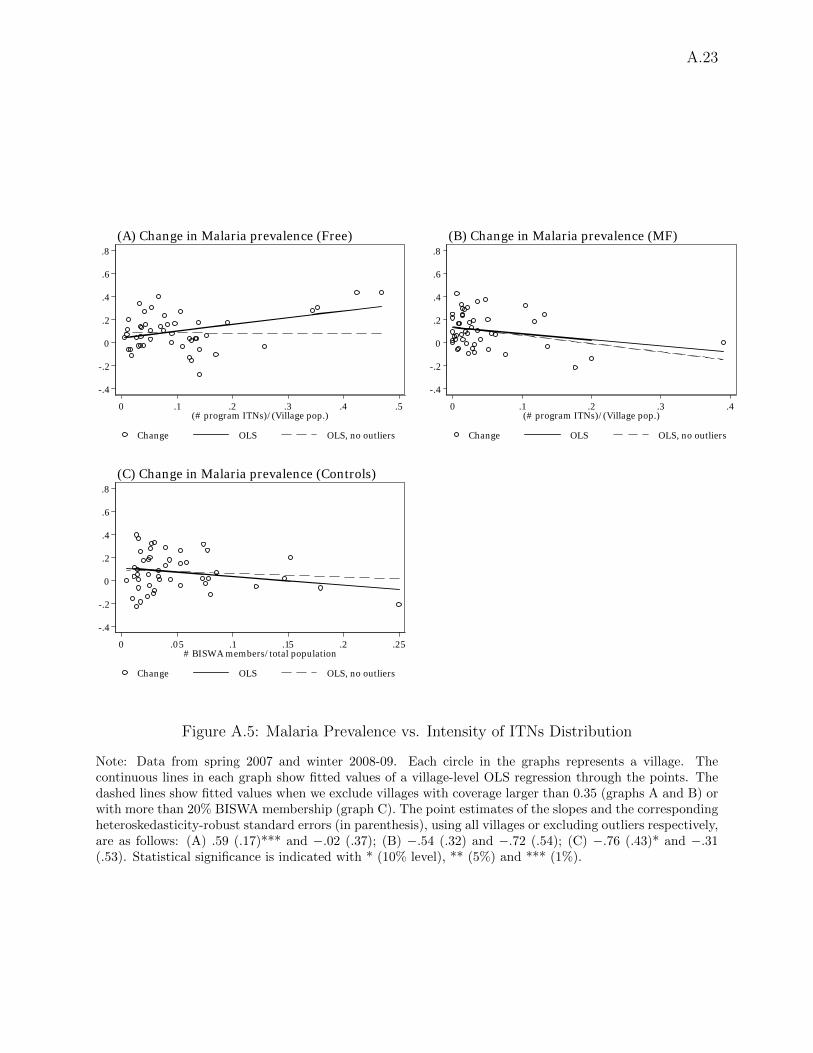
As a first step, we estimated village-specific changes in malaria prevalence in all interventioncommunities. We then plot the results against a measure of village-wide ITN coverage, calculated asthe ratio of the total number of ITNs distributed to BISWA households (regardless of their inclusionin the survey sample) and village population counts from the 2001 Indian Census. Although notup-to-date, the population counts are a good proxy for current population, and if anything, in mostcases 2001 population would underestimate current population, so that our estimates may overstatetrue coverage. The results are displayed separately for MF and Free communities in the two panelsat the top of Figure A.5. Each graph also shows the fitted values of two OLS regressions, one wherewe include data from all villages (the continuous line) and the other where we exclude the very fewvillages where the ITN coverage ratio was larger that 0.35 (the dashed lines).
When we include all Free villages, there is a positive association between malaria prevalenceat follow-up and program coverage. The estimated slope (0.59) is actually significant at the 1%level. However, the results are driven by the three outlier villages with coverage > 0.35, and whenwe exclude them the slope becomes negative but very close to zero (−0.02) and not significant atstandard levels (p-value = 0.966). In MF villages (panel B), where substantially fewer ITNs weredistributed, the slope of the regressions are negative but we cannot reject the null that slopes arezero at standard levels, although when we include all villages the slope is almost significant at the10% level (p-value = 0.103).
Because the ITN coverage achieved in MF communities was endogenously determined by house-hold purchase decisions, its association with changes in malaria prevalence should not be interpretedas necessarily causal. In contrast, in communities with free distribution, the number of ITNs de-livered was decided by our research team based on household size and composition. This producedvariation in ITN coverage resulting only from the distribution of BISWA affiliation and householdcomposition within the community. Even so, BISWA affiliation could be associated with villagecharacteristics related to malaria prevalence, although if we regress malaria prevalence at baselineon ITN coverage the slope is close to zero (0.03) and not significant (p-value = 0.720). On the onehand, the fact that the dependent variable in panels A and B is the change in prevalence, elimi-nates any possible spurious correlation due to time-invariant (observed or unobserved) village-levelcharacteristics. On the other hand, there may be other unobserved differences in trends correlatedwith both ITN coverage and malaria prevalence. To address this concern, in panel C of FigureA.5 we look at the relationship between changes in prevalence and the fraction of the populationaffiliated to BISWA in control villages (“BISWA penetration”). No ITNs were distributed in thesecommunities, but by construction BISWA penetration is very strongly correlated with the measureof ITN coverage that would have been observed if ITNs had been distributed as in Free commu-nities. Indeed, the correlation between the two variables in Free villages is 0.95. The graph inpanel C shows no clear association between changes in malaria prevalence and BISWA penetration.This suggests, albeit indirectly, that the lack of an association between changes in prevalence andITN coverage in Free villages (panel A) is unlikely to be caused by differential trends in prevalenceacross communities with varying degrees of BISWA penetration.
As an additional check, we use Control and Free villages to estimate an OLS regression of the
32We could not study the link between prevalence and density of ITNs throughout the village (e.g. thenumber of ITNs per squared hectare), because we do not have information on village size. The Indian Censusreports the area covered by each village, but it does not report the size and the distribution of the areascovered by dwellings. In Section A.16 we look at the link between prevalence and coverage within the villageusing data from a subset of communities where we collected GIS information for all households.
A.14
village-level change in prevalence on BISWA penetration, the Free dummy, and the interactionbetween the two variables. If ITN coverage were causing declines in malaria prevalence in oursample, we would expect the coefficient on the interaction to be negative. Consistent with theresults in panel A, we find instead that the coefficient is positive and significant when we include all94 villages (= 1.8, p-value= 0.009), and close to zero and not significant (= 0.25, p-value= 0.770)when we exclude the three villages with coverage larger than 0.35. Overall, we conclude that in oursample the coverage of the intervention did not appear to be systematically related to the changesin malaria prevalence.
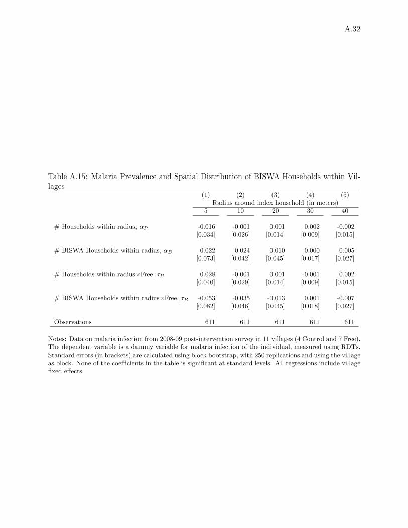
A.16 Within-village Externalities
In Section A.15 we found no direct support for the link between ITN coverage and malaria preva-lence. In principle, it is still possible that such a link existed within villages, with more protectionprovided in clusters with a denser concentration of ITNs. Although the baseline and follow-upsurveys did not include geo-coding of household locations, such information was recorded later ina subset of 11 study villages, including four Control and seven Free villages. The geo-coding wascompleted in February-June 2012, during the implementation of the supplemental Cash arm de-scribed in Section 3.2.1. Unfortunately, time and funding constraints did not allow us to conduct acomplete mapping of the whole study area. In this section we show that the available data providesome evidence of within-village externalities, although the estimates are very imprecise and the nullof no effect can never be rejected.
In each of the 11 villages, surveyors visited all households, regardless of BISWA affiliation, andrecorded for each latitude and longitude using GPS hardware.33 Surveyors also recorded whetherthe household belonged to BISWA at the time of the baseline survey, in 2007. Although the GPSsurvey was carried out a few years later, we were able to find nearly all of the original surveyedhouseholds and field observations suggested that few households had moved within the village sowe are reasonably confident that the 2012 GPS coordinates are accurate measures of households’2007-2009 locations.
We then constructed measures of population density within pre-specified radii of our samplehouseholds. Concretely, for each sample household (an ‘index’ household) we constructed thetotal number of neighbors (P ) and the number of BISWA households (B) within a given radius.The number of BISWA households matters because they all received ITNs in the Free villages,so that B provides a good proxy for the potential ITN coverage around the index household.Controlling for total population in the neighborhood is important, because B is by constructionstrongly correlated with population density around the index household, and this in turn may becorrelated with unobserved characteristics that could be linked to health. On average householdshad 16 neighbors within a 20-meter radius, of whom 7 were BISWA members.
We thus estimate the following model for the malaria indicator Miv of individual i in village v:
where αv is a village fixed effect, and Freev is the usual dummy for Free villages. The inclusion ofControl villages allows to interpret the estimates of τP and τB as causal, because any correlationbetween malaria infection and population density regardless of ITN presence will be captured by
33For each location, two independent measurements were taken, and both were recorded. This doublemeasurement allowed to detect a handful of measurement errors, but otherwise the vast majority of mea-surements were almost identical, so the results remain virtually unchanged if we use either one or the othersets of records.
A.15
αP and αB. In particular, if there are externalities from being surrounded by households withITNs, we expect τB < 0, that is, after controlling for total density P , an increase in the number ofBISWA neighbors should be associated with lower malaria prevalence in Free relative to Controlvillages. In contrast, we do not have clear predictions for the sign of τP , which measures the impactof population density regardless of ITN coverage. Note that the interpretation of τB as measuringexternalities needs to be taken with caution, given that the number of BISWA neighbors, even whencontrolling for overall density, was not randomly determined, and may proxy for other unobservedlocation characteristics.34
Overall, we have malaria infection status for 611 individuals, but because identification relieson individual variation in neighbors interacted with treatment status, we cluster standard errorsat the village level. Because we have only 11 villages, we estimate standard errors using blockbootstrap, using the village as the block in each iteration. We only focus on relatively short radii,because several of the villages are small, and using a radius of 50 meters or more would generatecollinearity between the measures of density and the village fixed effects, reducing further thealready small number of observations. Table A.15 displays the results, which show some evidenceof externalities at short ranges, from 5 to 20 meters, although the estimates are very impreciseand the null of no correlation is never rejected at standard levels. The estimated τB becomes closeto zero for distances of 30 or 40 meters, but the point estimates are relatively large if we look athouseholds immediately around the index households. For instance, If we compare two householdsin Free villages with an average number of total neighbors within a 10m radius (5.7), but with 0versus 2.6 (the average) BISWA members among them, the predicted probability of malaria will be2.6× 0.035 = 9 percentage points lower in the household with more BISWA neighbors, relative towhat would be predicted in Control areas. Of course, the 95% confidence interval is large, so thenull of no relationship, or even of a positive relationship between ITN coverage and malaria cannotbe rejected.
Appendix Bibliography
Adhvaryu, A. (2012). Learning, misallocation, and technology adoption: Evidence from new malariatherapy in Tanzania. Working Paper.
Ashraf, N., J. Berry, and J. Shapiro (2010). Can higher prices stimulate product use? Evidencefrom a field experiment in Zambia. American Economic Review 100 (5), 2383–2413.
Beier, J., G. Killeen, and J. Githure (1999). Short report: entomologic inoculation rates andplasmodium falciparum malaria prevalence in africa. The American Journal of Tropical Medicineand Hygiene 61 (1), 109–113.
Binka, F., F. Indome, and T. Smith (1998). Impact of spatial distribution of permethrin-impregnated bed nets on child mortality in rural northern Ghana. The American Journal ofTropical Medicine and Hygiene 59 (1), 80–85.
Charlwood, J. and P. Graves (1987). The effect of permethrin-impregnated bednets on a populationof Anopheles farauti in coastal Papua New Guinea. Medical and veterinary entomology 1 (3),319–327.
34So, for instance, our specification is not identical to that in Miguel and Kremer (2004) or Dupas (2012b),because in both these studies the fraction of treated neighbors was randomized by design.
A.16
Cohen, J. and P. Dupas (2010). Free distribution or cost-sharing? Evidence from a randomizedmalaria prevention experiment. Quarterly Journal of Economics 125 (1), 1–45.
Cohen, J., P. Dupas, and S. G. Schaner (2012). Price subsidies, diagnostic tests, and targetingof malaria treatment: Evidence from a randomized controlled trial. NBER Working Paper No.17943.
Delavande, A., X. Gine, and D. McKenzie (2010). Measuring subjective expectations in developingcountries: A critical review and new evidence. Journal of Development Economics 94 (2), 151–163.
Dupas, P. (2012). Short-run subsidies and long-run adoption of new health products: Evidencefrom a field experiment. Working Paper.
Enayati, A. and J. Hemingway (2010). Malaria management: Past, present, and future. AnnualReview of Entomology 55 (1), 569–591.
Farcas, G. A., K. J. Y. Zhong, F. E. Lovegrove, C. M. Graham, and K. C. Kain (2003). Evaluationof the Binax now(r) ict test versus polymerase chain reaction and microscopy for the detection ofmalaria in returned travelers. The American Journal of Tropical Medicine and Hygiene 69 (6),589–592.
Hawley, W. A., P. A. Phillips-Howard, F. O. ter Kuile, D. J. Terlouw, J. M. Vulule, M. Ombok, B. L.Nahlen, J. E. Gimnig, S. K. Kariuki, M. S. Kolczak, and A. W. Hightower (2003). Community-wide effects of permethrin-treated bed nets on child mortality and malaria morbidity in westernKenya. The American Journal of Tropical Medicine and Hygiene 68 (4 Suppl), 121–7.
Humar, A., C. Ohrt, M. A. Harrington, D. Pillai, and K. C. Kain (1997). Parasight(R)F testcompared with the polymerase chain reaction and microscopy for the diagnosis of Plasmodiumfalciparum malaria in travelers. The American Journal of Tropical Medicine and Hygiene 56 (1),44–48.
Khairnar, K., D. Martin, R. Lau, F. Ralevski, and D. Pillai (2009). Multiplex real-time quanti-tative PCR, microscopy and rapid diagnostic immuno-chromatographic tests for the detectionof Plasmodium spp: performance, limit of detection analysis and quality assurance. MalariaJournal 8 (1), 284.
Killeen, G. F., T. A. Smith, H. M. Ferguson, H. Mshinda, S. Abdulla, C. Lengeler, and S. P.Kachur (2007). Preventing childhood malaria in Africa by protecting adults from mosquitoeswith insecticide-treated nets. PLoS Medicine 4 (7).
Kremer, M. and E. Miguel (2007). The illusion of sustainability. Quarterly Journal of Eco-nomics 122 (3), 1007–1065.
Magesa, S., T. Wilkes, A. Mnzava, K. Njunwa, J. Myamba, M. Kivuyo, N. Hill, J. Lines, andC. Curtis (1991). Trial of pyrethroid impregnated bednets in an area of Tanzania holoendemicfor malaria. Part 2. Effects on the malaria vector population. Acta Tropica 49, 97–108.
Mbogo, C. N. M., N. M. Baya, A. V. O. Ofulla, J. I. Githure, and R. W. Snow (1996). Theimpact of permethrin-impregnated bednets on malaria vectors of the Kenyan coast. Medical andVeterinary Entomology 10 (3), 251–259.
Miguel, E. and M. Kremer (2004). Worms: identifying impacts on education and health the presenceof treatment externalities. Econometrica 72 (1), 159–217.
Mishra, A. K., S. K. Chand, T. K. Barik, V. K. Dua, and K. Raghavendra (2012). Insecticideresistance status in Anopheles culicifacies in Madhya Pradesh, central India. Journal of VectorBorne Diseases 49 (1), 39–41.
Moiroux, N., M. B. Gomez, C. Pennetier, E. Elanga, A. Djenontin, F. Chandre, I. Djegbe, H. Guis,
A.17
and V. Corbel (2012). Changes in Anopheles funestus biting behaviour following universal cov-erage of long-lasting insecticidal nets in Benin. Journal of Infectious Diseases.
Moody, A. (2002). Rapid diagnostic tests for malaria parasites. Clinical Microbiology Reviews 15 (1),66–78.
Pates, H. and C. Curtis (2005). Mosquito behavior and vector control. Annual Review of Entomol-ogy 50, 53–70.
Sahu, S. S., K. Gunasekaran, and P. Jambulingam (2009). Bionomics of Anopheles minimus and An.fluviatilis (Diptera: Culicidae) in East-central India, endemic for falciparum malaria: Humanlanding rates, host feeding, and parity. Journal of Medical Entomology 46 (5), 1045–1051.
Sharma, S., A. Upadhyay, B. Kindo, M. Haque, and P. Tyagi (2012). Impact of changing over ofinsecticide from synthetic pyrethroids to DDT for indoor residual spray in a malaria endemicarea of Orissa, India. The Indian Journal of Medical Research 135 (3), 382–388.
Sharma, S. K., P. K. Tyagi, K. Padhan, A. K. Upadhyay, M. A. Haque, N. Nanda, H. Joshi,S. Biswas, T. Adak, B. S. Das, V. S. Chauhan, C. E. Chitnis, and S. K. Subbarao (2006).Epidemiology of malaria transmission in forest and plain ecotype villages in Sundargarh Districtand Orissa, India. Transactions of the Royal Society of Tropical Medicine and Hygiene 100 (10),917–925.
Sharma, S. K., A. K. Upadhyay, M. A. Haque, O. P. Singh, T. Adak, and S. K. Subbarao (2004).Insecticide susceptibility status of malaria vectors in some hyperendemic tribal districts of Orissa.Current Science 87 (12), 1722–1726.
Smith, D., C. Guerra, R. Snow, and S. Hay (2007). Standardizing estimates of the Plasmodiumfalciparum parasite rate. Malaria Journal 6 (1), 131.
Takken, W. (2002). Do insecticide-treated bednets have an effect on malaria vectors? TropicalMedicine & International Health 7 (12), 1022–1030.
Tarozzi, A., A. Mahajan, B. Blackburn, D. Kopf, L. Krishnan, and J. Yoong (2011). Micro-loans,bednets and malaria: Evidence from a randomized controlled trial in Orissa (India). WorkingPaper, available at http://www.econ.upf.edu/~tarozzi/TarozziEtAl2011RCT.pdf.
Thomas, D., E. Frankenberg, J. Friedman, J.-P. Habicht, M. Hakimi, N. Ingwersen, Jaswadi,N. Jones, K. McKelvey, G. Pelto, B. Sikoki, T. Seeman, J. P. Smith, C. Sumantri, W. Suriastini,and S. Wilopo (2006). Causal effect of health on labor market outcomes: Experimental evidence.Working Paper.
Trape, J.-F., A. Tall, N. Diagne, O. Ndiath, A. B. Ly, J. Faye, F. Dieye-Ba, C. Roucher,C. Bouganali, A. Badiane, F. D. Sarr, C. Mazenot, A. Toure-Balde, D. Raoult, P. Druilhe,O. Mercereau-Puijalon, C. Rogier, and C. Sokhna (2011). Malaria morbidity and pyrethroid re-sistance after the introduction of insecticide-treated bednets and artemisinin-based combinationtherapies: a longitudinal study. The Lancet Infectious Diseases 11 (12), 925–932.
van den Broek, I., O. Hill, F. Gordillo, B. Angarita, P. Hamade, H. Counihan, and J.-P. Guthmann(2006). Evaluation of three rapid tests for diagnosis of P. falciparum and P. vivax malaria incolombia. The American Journal of Tropical Medicine and Hygiene 75 (6), 1209–1215.
World Health Organization (2002). Instructions for treatment and use of insecticide-treatedmosquito nets. WHO/CDS/RBM 2002.41, World Health Organization, Geneva, Switzerland.
World Health Organization (2005). Safety of pyrethroid for public health use.WHO/CDS/WHOPES/GCDPP/2005.10, WHO/PCS/RA/2005.1, Communicable DiseaseControl, Prevention and Eradication WHO Pesticide Evaluation Scheme (WHOPES) &Protection of the Human Environment Programme on Chemical Safety (PCS).
Yadav, R. S., R. R. Sampath, and V. P. Sharma (2001). Deltamethrin treated bednets for control ofmalaria transmitted by Anopheles culicifacies (Diptera: Culicidae) in India. Journal of MedicalEntomology 38 (5), 613–622.
Zwane, A. P., J. Zinman, E. V. Dusen, W. Pariente, C. Null, E. Miguel, M. Kremer, D. S. Karlan,R. Hornbeck, X. Gine, E. Duflo, F. Devoto, B. Crepon, and A. Banerjee (2011). Being surveyedcan change later behavior and related parameter estimates. Proceedings of the National Academyof Sciences 108 (5), 1821–1826.
A.19
Study Design: Location
Malaria: “number one public health problem” in Orissa (OHDR, 2004)
2003 Dept of Health and Family Welfare data show 417,000 cases of malaria (83%falciparum).
High % of self-reported malaria (NFHS-1999) in our study districts: 8.5% inSambalpur and Bargarh, 8.8% in Balangir, 12.3% in Keonjhar, 17.2% in Phulbani.
Tarozzi et al. (Duke, RAND and Stanford) Micro-loans, Bednets and Malaria April 2009 1 / 1
Figure A.1: Study AreasNotes: Study communities at baseline included 30 villages in Sambalpur, 9 in Khandhamal, 30 in Keonjhar(Kendujhar), 33 in Balangir and 48 in Bargarh. Nine villages were later excluded from the analysis becausethe baseline survey showed that BISWA had no active presence there (5 villages in Sambalpur and 4 inBalangir).
0.2
.4.6
.8
U5 15 to 45 45 or olderFemale Male Female Male Female Male
Anemia (Hb<11) Malaria
Figure A.2: Baseline Malaria and Anemia Prevalence, by Demographic GroupNotes: Data from Spring 2007 baseline survey. The bars represent the results of blood testing for anemia(n = 2, 532) and malaria (n = 2, 561) prevalence.
A.20
0.1.2.3.4.5
0-4
5-14
15-5
9>
=60
Age
gro
up
CM
FFr
ee
A. M
alaria
Pre
valen
ce, M
ales
0.1.2.3.4.5
0-4
5-14
15-5
9>
=60
Age
gro
up
CM
FFr
ee
B. M
alaria
Pre
valen
ce, F
emale
s0.2.4.6.81
0-4
5-14
15-5
9>
=60
Age
gro
up
CM
FFr
ee
C. A
nem
ia (H
b<11
g/dl
) Pre
valen
ce, M
ales
0.2.4.6.81
0-4
5-14
15-5
9>
=60
Age
gro
up
CM
FFr
ee
D. A
nem
ia (H
b<11
g/dl
) Pre
valen
ce, F
emale
s
Fig
ure
A.3
:P
ost-
inte
rven
tion
Mal
aria
and
Anem
iaP
reva
lence
,by
Age
and
Gen
der
Not
es:
Col
um
ns
show
anem
iaor
mal
aria
pre
vale
nce
inth
esp
ecifi
cage-
gen
der
gro
up
,by
exp
erim
enta
larm
.E
ach
colu
mn
als
od
isp
lays
95%
con
fid
ence
inte
rval
s,ro
bu
stto
intr
a-vil
lage
corr
elat
ion
.
A.21
A.22
A. Usage 90% B. Usage 45%
Coverage rate Coverage rate
Rel
ati
ve
Tra
nsm
issi
on I
nte
nsi
ty
Figure A.4: Figure 1: Protective Power of ITNs vs. Community Coverage
Source: Calculations from the epidemiological model in Killeen et al. (2007). The graphs can be pro-duced using the spreadsheet provided by Killeen et al. at http://www.ncbi.nlm.nih.gov/pmc/articles/PMC1904465/bin/pmed.0040229.sd001.xls. Coverage is defined as the fraction of individuals using an ITNeach night, while the relative transmission intensity is the proportional reduction of infectious bites for users(continuous lines) and non-users (dashed line in graph A). The label ‘usage’ refers to the fraction of time ofnormal exposure during which the individual is actually protected by the ITN.
0 .05 .1 .15 .2 .25# BISWA members/total population
Change OLS OLS, no outliers
(C) Change in Malaria prevalence (Controls)
Figure A.5: Malaria Prevalence vs. Intensity of ITNs Distribution
Note: Data from spring 2007 and winter 2008-09. Each circle in the graphs represents a village. Thecontinuous lines in each graph show fitted values of a village-level OLS regression through the points. Thedashed lines show fitted values when we exclude villages with coverage larger than 0.35 (graphs A and B) orwith more than 20% BISWA membership (graph C). The point estimates of the slopes and the correspondingheteroskedasticity-robust standard errors (in parenthesis), using all villages or excluding outliers respectively,are as follows: (A) .59 (.17)*** and −.02 (.37); (B) −.54 (.32) and −.72 (.54); (C) −.76 (.43)* and −.31(.53). Statistical significance is indicated with * (10% level), ** (5%) and *** (1%).
Tab
leA
.7:
Com
par
ison
ofSam
ple
Villa
ges
vs.
Ove
rall
Villa
geP
opula
tion
inStu
dy
Dis
tric
ts
(1)
(2)
(3)
(4)
(5)
(6)
(7)
Mea
ns,
by
villa
geca
tego
ryno.
ofT
ests
(p-v
alues
)N
otin
sam
ple
Con
trol
,n
=47
Fre
e,n
=47
MF
,n
=47
Villa
ges
H0:
All
H0:
Exp
er.
equal
arm
seq
ual
Are
aof
Villa
ge(i
nhec
tare
s)27
5.2
413.
147
6.4
417.
489
910.
000*
**0.
608
Num
ber
ofH
ouse
hol
ds
121.
526
1.4
359.
028
4.3
8991
0.00
0***
0.52
6Sch
edule
dC
aste
pop
ula
tion
(%)
0.13
40.
164
0.16
40.
173
8630
0.01
2**
0.92
1Sch
edule
dT
rib
ep
opula
tion
(%)
0.47
80.
328
0.37
20.
321
8630
0.00
0***
0.59
7F
emal
es0.
501
0.49
70.
496
0.49
986
300.
128
0.76
3P
rim
ary
school
0.74
60.
936
0.97
90.
936
8991
0.00
0***
0.43
2M
iddle
school
0.23
60.
383
0.59
60.
447
8991
0.00
0***
0.09
6*Sec
ondar
ysc
hool
0.12
90.
319
0.40
40.
298
8991
0.00
0***
0.52
3H
ospit
al0.
002
0.00
00.
021
0.00
089
910.
001*
**0.
312
Num
ber
ofP
rim
ary
Hea
lth
Cen
tres
0.02
50.
106
0.06
40.
064
8991
0.13
20.
712
Num
ber
ofP
rim
ary
Hea
lth
Sub
Cen
tres
0.10
50.
170
0.23
40.
213
8991
0.02
9**
0.72
7W
ell
Wat
er0.
815
0.83
00.
872
0.80
989
910.
692
0.67
8T
ank
Wat
er0.
557
0.70
20.
723
0.74
589
910.
000*
**0.
899
Riv
erW
ater
0.12
00.
106
0.17
00.
149
8991
0.74
70.
643
Can
al0.
050
0.12
80.
149
0.12
889
910.
034*
*0.
943
Num
ber
ofP
ost
Offi
ce0.
158
0.23
40.
383
0.25
589
910.
003*
**0.
246
Num
ber
ofT
elep
hon
eco
nnec
tion
s0.
285
0.53
20.
617
0.55
389
910.
000*
**0.
682
Bus
serv
ices
0.22
80.
255
0.29
80.
298
8991
0.49
90.
866
Num
ber
ofC
omm
erci
alB
anks
0.02
70.
064
0.06
40.
085
8991
0.24
20.
906
Num
ber
ofA
gric
ult
ura
lC
redit
Soci
etie
s0.
027
0.08
50.
106
0.10
689
910.
043*
*0.
919
Appro
ach
-P
aved
Roa
d0.
332
0.38
30.
426
0.36
289
910.
506
0.81
3D
ista
nce
from
the
nea
rest
Tow
n(i
nK
ilom
eter
s)34
.934
.325
.226
.189
910.
000*
**0.
445
Ele
ctri
city
for
Dom
esti
cuse
0.46
50.
702
0.57
50.
681
8991
0.00
0***
0.38
9E
lect
rici
tyof
Agr
icult
ura
luse
0.06
60.
106
0.06
40.
149
8991
0.34
60.
386
Wet
Ric
e(i
rrig
ated
)cu
ltiv
ated
Are
a(%
)0.
075
0.15
10.
188
0.18
388
750.
000*
**0.
727
Dry
Ric
e(n
otir
riga
ted)
cult
ivat
edA
rea
(%)
0.42
20.
504
0.48
30.
510
8875
0.00
5**
0.86
4
Not
es:
Dat
afr
omth
e20
01G
over
nm
ent
ofIn
dia
Cen
sus.
Th
ep
oin
tes
tim
ate
sin
colu
mn
1in
dic
ate
mea
ns
invil
lages
not
incl
ud
edin
the
base
lin
esa
mp
le,
wh
ile
esti
mat
esin
colu
mn
s2
to4
ind
icate
mea
ns
inst
udy
vil
lages
that
bel
on
gto
the
gro
up
ind
icate
din
the
colu
mn
hea
der
.T
he
figu
res
inco
lum
n6
are
p-v
alu
esfo
rth
enu
llhyp
oth
esis
that
the
mea
nof
the
vari
ab
lein
the
row
isth
esa
me
acr
oss
all
fou
rvil
lage
gro
up
s.T
he
p-v
alu
esin
colu
mn
7ar
efo
rth
ete
stof
equ
alit
yam
ong
the
thre
eex
per
imen
tal
arm
s.S
tati
stic
al
sign
ifica
nce
isin
dic
ate
das
***
(1%
leve
l),
**
(5%
)or
*(1
0%
).A
llte
sts
are
het
eros
ked
asti
city
-rob
ust
.
A.24
A.25
Table A.8: Attrition between Pre and Post Intervention Household Surveys
Dependent variable: Dummy = 1 if household (1) (2) (3) (4)was not re-interviewed at follow-up
Notes: OLS estimates. Standard errors (in brackets) are robust to intra-village correlation. Asterisks indicatesignificance at the 10 (*), 5 (**) and 1% (***) level. All regressions include observations from 141 clusters(villages). The smaller sample size in columns 3 and 4 relative to columns 1 and 2 is due to missing valuesin one or more regressors.
A.26
Table A.9: Tests of Balance for Characteristics of Cash Villages (p-values)(1) (2) (3)
Cash vs. Cash: Cash:Other Study New vs. Low vs.
villages Control High price
Area of Village (in hectares) 0.862 0.822 0.196Number of Households 0.961 0.997 0.077*SC population (%) 0.378 0.221 0.785ST population (%) 0.006 0.627 0.476Females 0.884 0.931 0.964Middle school in village 0.78 0.752 0.539Secondary school in village 0.594 0.68 0.108Primary Health Centre 0.9 0.08* 0.56Primary Health Sub Centre 0.642 0.262 0.267Well Water 0.224 0.573 1Tank Water 0.046** 0.213 1River Water 0.68 0.283 0.222Canal 0.589 0.283 0.687Post Office 0.637 0.933 0.096*Telephone connection 0.836 0.874 1Bus services 0.393 0.623 0.194Agricultural Credit Societies 0.693 0.08* 0.56Paved Road 0.063* 0.066* 0.214Distance from the nearest Town (in Kms) 0.18 0.807 0.75Electricity for Domestic use 0.119 0.378 1Electricity of Agricultural use 0.719 0.906 0.643Wet Rice (irrigated) cultivated Area (%) 0.892 0.324 0.518Dry Rice (un-irr.) cult. Area (%) 0.41 0.342 0.741
# Villages 156 40 40
Notes: all figures are p-values of tests of equality of means of the listed village-level characteristics betweenvillages in the two groups indicated in the column header. All data are from the 2001 Census of India. Alltests are heteroskedasticity-robust. Asterisks denote statistical significance at the 10(*), 5(**) or 1%(***)level. The results in column (1) use information from the 40 Cash villages and from the remaining 116villages surveyed at baseline (47 MF, 47 Free and the 22 Control villages not included in the Cash study as‘PC’ villages). The results in column 2 use information from the 25 PC villages and the 15 New villages.The same 40 villages are also used in column 3, where they are split by whether LLINs were sold at loweror higher prices (20 per group).
Notes: Data from post-intervention household survey (Winter 2008-09). Standard errors (in brackets) arerobust to intra-village correlation. Asterisks indicate significance at the 10 (*), 5 (**) and 1% (***) level.All figures are OLS estimates of a linear probability model where the dependent variable is indicated inthe column header. Both absence and refusal refer to malaria RDTs, but the figures for Hb are almostidentical. All regressions include only observations from all members (at the time of the follow-up) of the1768 households interviewed at baseline and re-contacted during the follow-up survey.
A.28
Table A.11: Results of Rapid Diagnostic Tests Validation
RDT(1) RDT(2) RDT(3)
RDT(2) 0.7873RDT(3) 0.7844 0.8760
Microscopy 0.5274 0.6131 0.5968
Microscopy-ve +ve
Tester 1 -ve 129 1RDT +ve 45 30
Microscopy-ve +ve
Tester 2 -ve 148 3RDT +ve 26 28
Microscopy-ve +ve
Tester 3 -ve 146 3RDT +ve 28 28
Notes: Data from July 2009. The results refer to tests of 205 blood samples collected from individuals withmalaria symptoms in 3 villages in Rourkela district (Orissa). The figures in the sub-table on top are samplecorrelations between the results as read by the tester indicated in the column header and the one indicated inthe row. The figures in the three sub-tables underneath indicate the details of the sample joint distributionsof the test results as read by each tester vs. microscopy. Testers 1 and 2 were part of the field team thatconducted blood tests during the follow-up household survey. Tester 3 was the most senior survey monitorin the team.
A.29
Table A.12: Knowledge of Causes of Malaria and Risk Mitigating Behavior
Inner walls sprayed in 2008-09 0.403 0.368 0.296 0.242Outer walls sprayed in 2008-09 0.531 0.481 0.442 0.575
(D) Number of nets from other sources in the 12 months before the follow-up survey (per head)
From Government/health centers 0.051 0.054 0.136 0.321From NGOs other than BISWA 0.004 0.000 0.019 0.328Purchased from the market 0.678 0.139 0.511 0.000***
Notes: Data from follow-up survey (winter 2008-09). Only panel households are included (n = 1, 768).The figures in panels A and B show proportions of respondents who list, un-prompted, the cause/behaviorindicated in the row header. The p-values in column 4 are calculated for a test of the joint null hypothesisthat means are identical across experimental arms. All tests are robust to the presence of intra-villagecorrelation of residuals. Asterisks in column 4 indicate significance at the 10 (*), 5 (**) and 1% (***) level.
Tab
leA
.13:
Sel
f-re
por
ted
Mal
aria
Indic
es:
Bas
elin
ean
dF
ollo
w-u
pD
iffer
ence
sin
Lev
els
(1)
(2)
(3)
(4)
(5)
(6)
(7)
(8)
(9)
(10)
(11)
(12)
(13)
(14)
Cas
esw
ith
inN
um
ber
ofD
ays
ofw
ork
Hea
lth
Exp
end
itu
res
for
Cos
tsp
aid
Cos
tsp
aid
wit
ha
mon
thof
epis
od
esor
sch
ool
lost
exp
end
itu
res
dru
gs/d
oct
ors
wit
hdeb
tlo
wer
con
sum
pti
onsu
rvey
(las
t6
mon
ths)
(las
t6
mon
ths)
(las
t6
mon
ths)
(las
t6
mon
ths)
(las
t6
mon
ths)
(las
t6
mon
ths)
Bas
elin
eF
ollo
w-u
pB
asel
ine
Fol
low
-up
Bas
elin
eF
ollo
w-u
pB
asel
ine
Fol
low
-up
Bas
elin
eF
ollo
w-u
pB
asel
ine
Fol
low
-up
Bas
elin
eF
ollo
w-u
p
Sel
f-re
por
ted
Mal
aria
Fre
ed
istr
ibu
tion
=1
0.00
1-0
.001
0.03
2-0
.011
0.71
3-1
.231
189
-510
620
0.08
2-0
.033
0.09
3-0
.023
[0.0
02]
[0.0
03]
[0.0
15]*
*[0
.019
][0
.854
][1
.086
][1
21]
[178
][6
5][1
04]
[0.0
43]*
[0.0
51]
[0.0
53]*
[0.0
21]
Mic
ro-l
oan
s=1
0.00
20.
001
0.03
1-0
.018
0.92
-1.4
7516
3-1
0611
2-7
50.
032
-0.0
790.
090.
003
[0.0
03]
[0.0
03]
[0.0
15]*
*[0
.017
][0
.928
][0
.985
][1
31]
[161
][6
7]*
[86]
[0.0
33]
[0.0
45]*
[0.0
53]*
[0.0
26]
Con
stan
t(C
ontr
ol)
0.00
80.
007
0.09
20.
115
4.26
75.
779
625
863
318
487
0.15
10.
220.
244
0.06
9[0
.002
]***
[0.0
02]*
**[0
.009
]***
[0.0
13]*
**[0
.572
]***
[0.8
33]*
**[8
6]**
*[1
19]*
**[4
3]**
*[6
3]**
*[0
.022
]***
[0.0
38]*
**[0
.031
]***
[0.0
17]*
**
Ob
serv
atio
ns
9684
9598
9684
9598
1768
1768
1768
1768
1768
1768
1768
1768
1768
1768
Fre
e=M
F=
0(p
-val
ue)
0.69
920.
9247
0.04
02**
0.57
860.
5499
0.32
180.
2523
0.75
720.
1526
0.56
230.
1557
0.18
560.
111
0.40
74F
ree=
MF
(p-v
alu
e)0.
7803
0.69
310.
949
0.68
430.
8315
0.78
060.
8438
0.55
280.
929
0.35
480.
2648
0.27
550.
9574
0.26
88
Sel
f-re
por
ted
Mal
aria
and
Fev
erca
ses
Fre
ed
istr
ibu
tion
=1
0-0
.006
0.02
1-0
.049
-0.3
34-3
.213
8-2
1713
-75
0.05
4-0
.135
0.11
1-0
.057
[0.0
06]
[0.0
07]
[0.0
21]
[0.0
40]
[1.0
55]
[1.5
40]*
*[1
41]
[255
][8
0][1
45]
[0.0
60]
[0.1
11]
[0.0
89]
[0.0
74]
Mic
ro-l
oan
s=1
0.00
30.
005
0.04
1-0
.069
1.23
6-3
.571
230
-344
143
-193
0.03
2-0
.186
0.14
60.
013
[0.0
06]
[0.0
07]
[0.0
22]*
[0.0
37]*
[1.1
74]
[1.3
69]*
*[1
62]
[238
][9
0][1
32]
[0.0
59]
[0.1
17]
[0.0
86]*
[0.0
80]
Con
stan
t(C
ontr
ol)
0.02
60.
036
0.21
50.
458
7.84
713
.125
1,10
12,
011
566
1,11
10.
315
0.69
10.
613
0.26
2
[0.0
04]*
**[0
.005
]***
[0.0
15]*
**[0
.028
]***
[0.7
88]*
**[1
.190
]***
[108
]***
[184
]***
[62]
***
[99]
***
[0.0
40]*
**[0
.088
]***
[0.0
60]*
**[0
.055
]***
Un
itof
obse
rvat
ion
9684
9598
9684
9598
1768
1768
1768
1768
1768
1768
1768
1768
1768
1768
Fre
e=M
F=
0(p
-val
ue)
0.86
110.
2735
0.17
910.
1667
0.35
910.
0327
**0.
2735
0.35
350.
211
0.33
50.
6571
0.26
930.
2152
0.60
81F
ree=
MF
(p-v
alu
e)0.
6294
0.11
370.
3815
0.57
750.
1621
0.76
360.
1434
0.58
580.
1207
0.39
130.
7137
0.61
840.
7036
0.36
25
Not
es:
Dat
afr
ombas
elin
e(S
pri
ng
2007
)an
dp
ost
-inte
rven
tion
hou
seh
old
surv
eys
(Win
ter
2008-0
9).
All
resu
lts
are
OL
Ses
tim
ate
sof
diff
eren
ce-i
n-
diff
eren
ces
mod
els.
All
outc
omes
refe
rto
mal
aria
an
dfe
ver
epis
od
esd
iagn
ose
das
such
by
the
resp
on
den
t.M
on
etary
valu
esare
in2008-0
9R
up
ees.
Reg
ress
ion
sin
colu
mn
s1-
4ar
ees
tim
ated
atth
ein
div
idu
al
level
,w
hil
ere
gre
ssio
ns
5-1
4are
esti
mate
dat
the
hou
seh
old
leve
l.S
tan
dard
erro
rs(i
nb
rack
ets)
and
test
sar
ero
bu
stto
intr
a-vil
lage
corr
elati
on
.A
ster
isks
ind
icate
sign
ifica
nce
at
the
10
(*),
5(*
*)
an
d1%
(***)
level
.
A.30
A.31
Table A.14: Impact of Intervention on Self-reported Malaria and Fever Indices
(1) (2) (3) (4) (5) (6) (7)Malaria Malaria and fever episodes in 6 months before interviewor fever Number of Days of work Health expenditures # episodes # episodes paidprevious episodes or school lost All Doctors paid for for with lowermonth & drugs with debt consumption
Notes: Data from baseline (Spring 2007) and post-intervention household surveys (Winter 2008-09). Allresults are OLS estimates of difference-in-differences models. All outcomes refer to malaria and fever episodesdiagnosed as such by the respondent. Monetary values are in 2008-09 Rupees. Standard errors (in brackets)and tests are robust to intra-village correlation. Asterisks indicate significance at the 10 (*), 5 (**) and 1%(***) level.
A.32
Table A.15: Malaria Prevalence and Spatial Distribution of BISWA Households within Vil-lages
(1) (2) (3) (4) (5)Radius around index household (in meters)
Notes: Data on malaria infection from 2008-09 post-intervention survey in 11 villages (4 Control and 7 Free).The dependent variable is a dummy variable for malaria infection of the individual, measured using RDTs.Standard errors (in brackets) are calculated using block bootstrap, with 250 replications and using the villageas block. None of the coefficients in the table is significant at standard levels. All regressions include villagefixed effects.