Calculating Comparable Statistics from Incomparable Surveys, with an Application to Poverty in India Alessandro Tarozzi Duke University ∗ March 2003 Abstract We develop an intuitive and easily implemented procedure to recover comparability over time of statistics computed using databases made incomparable by changes in survey design. Our methodology can be adopted whenever the statistic of interest satisfies a certain simple moment condition. The moment condition is satisfied by many interesting economic indicators, including a broad range of poverty and inequality measures. The procedure we propose requires the existence of a set of auxiliary variables whose reports are not affected by the different survey design, and whose relation with the main variable of interest is stable across the surveys. The adjusted estimates can be recovered by using a two-step method of moments framework. Root-n consistency follows easily under regularity conditions. Because most household surveys adopt a multi-stage design, we provide expressions for the asymptotic variance which are robust to the presence of clustering and stratification. We use our adjustment procedure to estimate poverty counts from the 55 th Round of the Indian National Sample Survey, a large household survey carried out in 1999-2000. Due to important changes in the adopted questionnaire the unadjusted figures are likely to understate poverty relative to the previous rounds. We provide evidence supporting the plausibility of the identifying assumptions and we conclude that most of the very large reduction in poverty implied by the unadjusted figures is real. JEL: C13, C42, I32, O53 Key words: Poverty, Inequality, India, Method of Moments, Survey Methods. Address: Department of Economics, Duke University 305 Social Sciences Building - PO Box 90097 27708 Durham, NC. E-mail: [email protected]. ∗ I am grateful to Angus Deaton and Bo Honoré for comments, support, and conversations that led to this project. I would also like to thank Elie Tamer for his help, and for comments on an earlier draft, and Dwayne Benjamin, Debopam Bhattacharya, Phil Cross, Paul Ellickson, Allen Kelley, Peter Lanjouw, Aprajit Mahajan, Robert McMillan, Jonathan Morduch, and Barbara Rossi for comments and useful conversations, as well as seminar participants at Duke, Georgetown, Princeton, Toronto, Triangle Applied Microeconomics Conference, Villa Mondragone Workshop, and the World Bank. All errors are mine.
Transcript
Calculating Comparable Statistics from Incomparable Surveys,
with an Application to Poverty in India
Alessandro TarozziDuke University∗
March 2003
Abstract
We develop an intuitive and easily implemented procedure to recover comparability overtime of statistics computed using databases made incomparable by changes in survey design.
Our methodology can be adopted whenever the statistic of interest satisfies a certain simplemoment condition. The moment condition is satisfied by many interesting economic indicators,including a broad range of poverty and inequality measures. The procedure we propose requiresthe existence of a set of auxiliary variables whose reports are not affected by the different surveydesign, and whose relation with the main variable of interest is stable across the surveys. Theadjusted estimates can be recovered by using a two-step method of moments framework. Root-nconsistency follows easily under regularity conditions. Because most household surveys adopt amulti-stage design, we provide expressions for the asymptotic variance which are robust to thepresence of clustering and stratification. We use our adjustment procedure to estimate povertycounts from the 55th Round of the Indian National Sample Survey, a large household survey
carried out in 1999-2000. Due to important changes in the adopted questionnaire the unadjustedfigures are likely to understate poverty relative to the previous rounds. We provide evidencesupporting the plausibility of the identifying assumptions and we conclude that most of the verylarge reduction in poverty implied by the unadjusted figures is real.JEL: C13, C42, I32, O53Key words: Poverty, Inequality, India, Method of Moments, Survey Methods.Address:Department of Economics, Duke University305 Social Sciences Building - PO Box 9009727708 Durham, NC.
∗I am grateful to Angus Deaton and Bo Honoré for comments, support, and conversations that led to this project.
I would also like to thank Elie Tamer for his help, and for comments on an earlier draft, and Dwayne Benjamin,
Debopam Bhattacharya, Phil Cross, Paul Ellickson, Allen Kelley, Peter Lanjouw, Aprajit Mahajan, Robert McMillan,
Jonathan Morduch, and Barbara Rossi for comments and useful conversations, as well as seminar participants at Duke,
Georgetown, Princeton, Toronto, Triangle Applied Microeconomics Conference, Villa Mondragone Workshop, and
the World Bank. All errors are mine.
1 Introduction
Applied economists are often interested in studying changes over time of important economic indi-
cators, such as inequality, poverty, or aggregate measures of private consumption. However, such
comparisons are only meaningful insofar as the necessary data are collected consistently over time.
Poverty and inequality, in particular, are routinely evaluated using data from household surveys,
and it is common to observe changes in the questionnaire adopted by the statistical agency. How-
ever, the survey literature convincingly shows that revisions in the questionnaire can affect the
pattern of replies in important ways, so that changes in observed economic indicators sometimes
reflect changes in the survey, rather than real transformations of the economic environment.1
Several papers have recently highlighted the important consequences that the methodology
of data collection can have on the estimation of poverty and inequality. Gibson (1999) uses an
experiment carried out in Papua New Guinea to study the effects on poverty estimation of collecting
expenditure data using diaries instead of recall interviews. Gibson, Huang & Rozelle (2001, 2003)
note that changing the reference period in the Chinese Household Income and Expenditure Survey
would have dramatic effects on the estimation of poverty and inequality. Jolliffe (2001) studies the
large changes in poverty estimates for El Salvador that arise when the list of items included in the
expenditure questionnaire is changed. Lanjouw and Lanjouw (2001) perform a similar analysis for
Ecuador, Nepal, and Brazil. Others have analyzed the effect of the survey design in expenditure
surveys on the estimation of elasticities (Ghose and Bhattacharya, 1995) and economies of scale at
the household level (Gibson 2002).
This paper derives its main empirical motivation from a change in data collection methodology
that took place recently in India, stirring up an ongoing controversy on the poverty trends in this1See Deaton and Grosh (2000, part II) and references therein for an overview of the methodological issues involved
in collecting expenditure data.
2
country. Because of the still large proportion of poor households within the Indian population, the
local poverty numbers frequently appear in economic debates, not only in India, but also within the
World Bank. Poverty monitoring in India has historically been based on expenditure data, collected
approximately every five years in a large round of the Indian National Sample Survey (NSS). The
55th round of the NSS, carried out between July 1999 and June 2000, was awaited by many, with the
expectation that it would at least partly dispel the conflicting evidence on poverty reduction during
the nineties, which apparently conflicted with the high rates of economic growth that followed a
process of economic liberalization started in 1991.2 In 1993-94, at the time of the last quinquennial
survey carried out adopting the standard questionnaire, the proportion of the Indian population
estimated to be poor was 37.3 percent in the rural sector, and 32.4 percent in urban areas. In
1999-2000, the official poverty counts dropped to 27.1 and 23.6 respectively. However, there are a
priori arguments suggesting that the unadjusted figures are likely to understate poverty relatively
to the previous NSS rounds.
The reasons and consequences of the non-comparability of the 1999-2000 survey with previous
NSS rounds have already been analyzed elsewhere, and in the empirical section of the paper we
will only briefly summarize the main issues. In particular, the interested reader is referred to Datt,
Ravallion and Kozel (2003), Deaton (2001, 2003a, 2003b), Deaton and Drèze (2002), Sen (2000),
Sundaram and Tendulkar (2002, 2003) and Visaria (2000).
In this paper we develop an easily implemented adjustment procedure that reestablishes com-
parability over time for statistics estimated using surveys of different design. We also describe the
conditions under which the procedure will perform well, and we study the asymptotic properties
of the adjusted estimates in a method of moments framework. The main condition necessary to2The liberalization process started after a Balance of Payment crisis in the summer of 1991. See Sachs, Varshney,
and Bajpai (1999), and references therein.
3
achieve identification is the existence of a set of auxiliary variables whose reports are not affected
by the change in survey design, and whose relation with the main variable of interest is stable
across the surveys. We also show that the adjustment allows–with appropriate modifications–the
estimation of the full comparable distribution of a variable of interest.
The adjustment procedure has a simple intuition. Suppose, for example, that a researcher is
interested in estimating a poverty or inequality measure φ, which satisfies a population moment
condition E [m (y)− φ] = 0. Typically, y is a meausre of income or expenditure. If the parameter
of interest is a simple poverty headcount ratio, m (y) is a binary variable equal to one is y is below
the poverty line. Suppose that a change in the questionnaire makes the latest available data on
y non-comparable with analogous data collected in previous periods. Using the law of iterated
expectations, one can rewrite the moment condition as E [E [m (y)− φ | v]] , where v is a set of
auxiliary variables. Suppose that the change in the questionnaire did not affect the reports on v,
and that the conditional expectation in the latest survey is the same as in a previous one, which
adopted a standard questionnaire. Then one can recover a comparable estimate φ by estimating the
conditional expectation from the previous survey, and the marginal distribution from the current
one.
When the dimension of v is small, one can obtain the adjusted estimates nonparametrically.
Deaton (2003b) adopts this strategy to estimate adjusted poverty counts for the 55th round of the
Indian NSS using a single auxiliary variable. Specifically, he uses expenditure per head in a set of
miscellaneous items for which the recall period remained the same in all the NSS surveys. Ideally, it
would be useful to use also information on several household characteristics likely to be correlated
with y, but when the number of auxiliary variables is large, the use of nonparametric estimators
becomes computationally intractable. We show that the computational burden is greatly reduced
if one rewrites the estimator–through simple repeated application of Bayes’ rule–as a function of
4
conditional probabilities that can be estimated using a parametric binary dependent variable model.
This transformation implies that a broad spectrum of adjusted poverty and inequality measures
will satisfy a modified two step moment condition, with a logit first step. Since most household
surveys adopt a complex stratified and clustered design–which implies that observations are neither
independent not identically distributed–we study the asymptotic properties of the estimators using
the framework developed in Bhattacharya (2002), who studies the large sample properties of method
of moment estimators with multi-stage samples.
Clearly, the usefulness of the adjustment relies crucially on the identifying assumptions being
appropriate. Since such assumptions involve variables that are not observed, they cannot be for-
mally tested. In our application to the 1999-2000 round of the Indian NSS, we provide indirect
empirical support to the assumptions by making use of smaller experimental expenditure surveys,
carried out in years preceding the 55th round. We also show how these experimental surveys can be
used to test the performance of our adjustment procedure. Overall, the evidence suggests that our
estimates are useful to recover comparability across NSS rounds of different design. Surprisingly,
our results show that most of the reduction in poverty shown by the unadjusted figures is real,
even if the adjustment suggests that the change in the questionnaire actually caused a relative
underestimation of poverty rates, especially in rural areas.
Even if our emphasis on comparability issues over time is justified by the empirical application,
the approach developed here also has other potentially fruitful applications. For example, one
can merge information on auxiliary variables from a census (which commonly does not record
expenditure) with data on the same variables and expenditure from a household survey, to recover
welfare measures for geographically small areas, for which a representative sample from the survey
is typically not available.3 More generally, the estimator can be used to mitigate the problem of3For a different approach, see Elbers, Lanjouw and Lanjouw (2003), whose procedure explicitely focuses on the
5
missing data, when the statistic of interest satisfies a moment condition as the one described above,
and when data on an adequate set of auxiliary variables are available. Clearly, in every application
the plausibility of the identification assumptions should be carefully scrutinized.
The rest of the paper is organized as follows. Section 2 delineates the theoretical problem, and
states the assumptions required by our adjustment procedure. Section 3 introduces the estimator
and describes its asymptotic properties. We cover the empirical application in Section 4, and we
conclude in Section 5.
2 The Theoretical Problem
In what follows we will refer to the population sampled using a revised methodology as the target
population, while the auxiliary population is one that has been sampled using a standard question-
naire.4 Target and auxiliary surveys are analogously defined. Let τ be a binary variable equal
to one when an observation is drawn from the target population, and zero otherwise. Let y be
the main variable of interest as measured in a standard questionnaire. In poverty or inequality
measurement y typically measures consumption, income, or earnings per head.5 Suppose that the
researcher is interested in estimating the value of a parameter φ in a target population, where φ
satisfies the following population moment condition:
E [n (m (y)− φ) | τ = 1] = 0 (1)
estimation of micro-level poverty and inequality measures.4Typically there will be more than one potential auxiliary survey, one per every round of the survey carried out
before the changes in methodology.5Taking intra-household allocation into account would require controversial decisions on how to deal with household
scale economies and equivalence scales. For an overview of the issues involved see Deaton (1997, Ch. 4), and Deaton
and Case (2002).
6
where n is household size. The population moment (1) explicitely refers to the frequent situation
in which the parameter of interest is defined in terms of a per capita variable y across individuals,
but data are sampled at the household level. For example, φ might represent average calorie con-
sumption per head, so that m (y) = y, but the survey collects data on total household consumption.
When data are collected at the individual level, or when the parameter is not defined in per capita
terms, all the results that follow can be obtained as a straightforward special case with n = 1.
The moment condition (1) encompasses a broad set of commonly used poverty measures.6 For
example, if φ represents a Foster-Greer-Thorbecke (FGT) poverty index, and z is the poverty line,
then m (y) = 1(y < z)¡1− y
z
¢α, with α ≥ 0, where (1− y/z) represents the poverty gap, and 1(E)
is an indicator function equal to one when event E is true, and zero otherwise. When α = 0, the
index becomes the headcount poverty ratio, while α = 1 characterizes the poverty gap ratio. A
higher parameter α indicates that large poverty gaps (1− y/z) are given a larger weight in the
computation, so that the poverty index becomes more sensitive to the distribution of y among
the poor. The above moment condition is also easily adapted to describe well-known inequality
measures like the Atkinson index, ifm (y) =³
yE[y]
´1−², or the Theil index, withm (y) = y
E[y] lnyE[y] .
In these cases, the sample equivalent of equation (1) should contain a sample moment condition
for the expected value of y, which is generally not known.
Clearly, if y is not measured in the data collected from the target population, the estimation of
the parameter φ through the sample equivalent of (1) is infeasible. This is precisely the case if the
survey questionnaire changed in such a way that the respondents’ reports are no longer comparable
with those from previous surveys, so that the researcher can only observe a different variable, say
y, but not y. For example, y is consumption per head when the recall period is the week before the6For an introduction to the theory and practice of poverty measurement see Deaton (1997, Ch. 3). For poverty
estimation, see also Ravallion (1993).
7
interview, while y is the report corresponding to a different recall period. Since the phrasing of the
questions frequently have important effects on the pattern of replies, it should be clear that y and
y are actually different variables, even if they are purported to represent exactly the same object.
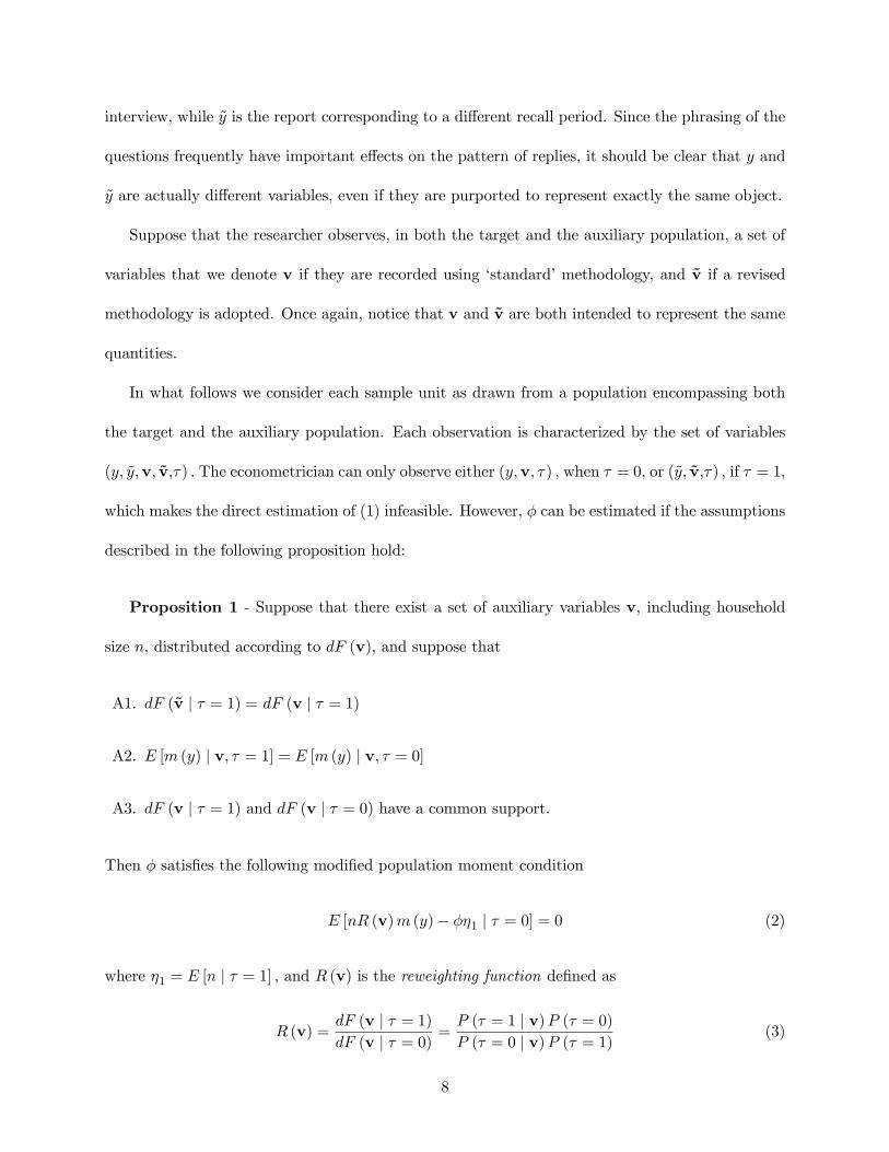
Suppose that the researcher observes, in both the target and the auxiliary population, a set of
variables that we denote v if they are recorded using ‘standard’ methodology, and v if a revised
methodology is adopted. Once again, notice that v and v are both intended to represent the same
quantities.
In what follows we consider each sample unit as drawn from a population encompassing both
the target and the auxiliary population. Each observation is characterized by the set of variables
(y, y,v, v,τ) . The econometrician can only observe either (y,v, τ) , when τ = 0, or (y, v,τ) , if τ = 1,
which makes the direct estimation of (1) infeasible. However, φ can be estimated if the assumptions
described in the following proposition hold:
Proposition 1 - Suppose that there exist a set of auxiliary variables v, including household
size n, distributed according to dF (v), and suppose that
A1. dF (v | τ = 1) = dF (v | τ = 1)
A2. E [m (y) | v, τ = 1] = E [m (y) | v, τ = 0]
A3. dF (v | τ = 1) and dF (v | τ = 0) have a common support.
Then φ satisfies the following modified population moment condition
E [nR (v)m (y)− φη1 | τ = 0] = 0 (2)
where η1 = E [n | τ = 1] , and R (v) is the reweighting function defined as
R (v) =dF (v | τ = 1)dF (v | τ = 0) =
P (τ = 1 | v)P (τ = 0)P (τ = 0 | v)P (τ = 1) (3)
8
where P (τ = 1 | v) is the probability that an observation belongs to the target population condi-
tional on observing v, and the other probabilities are defined accordingly.
Proof: see appendix.
Assumption A1 requires that the econometrician has access to a set of auxiliary variables v
whose marginal distribution is identified by the sampling process both in the auxiliary and in the
target population. In other words, v includes variables whose reports are left unaffected by the
change in survey design. Such variables are likely to be available, since questionnaire revisions
generally do leave several questions unchanged. When the non-comparability across surveys is
caused by changes in the methodology adopted to measure consumption or income, the inclusion
in v of household size and other household characteristics is reasonable, unless their definition
changes between surveys. A2 is the most crucial assumption, and the one who should be scrutinized
more closely in every empirical application of our methodology. It requires that the conditional
expectation of the function m (y) is the same in the target and the auxiliary surveys. For example,
if one is interested in estimating a headcount poverty ratio, A2 amounts to assuming that the
fraction of households to be counted as poor conditional on v remains constant across the two
surveys. Finally, the common support assumption A3 ensures that R (v) is finite and bounded
away from zero for each value of v, and that the distributions involved in A2 are defined for every
v. Intuitively, this condition ensures that we can estimate E [m (y) | v, τ = 1] for every v, which is
necessary in order to recover the unconditional population moment φ.7
The problem at hand has clear similarities with the problem of building counterfactuals for
causal inference with non-experimental data in program evaluation.8 In fact, the object we want to7Note that even if A3 does not hold one can still estimate bounds for the parameter of interest treating observations
with v outside the common support as missing values, using the setting described in Horowitz and Manski (1995).8For a review, see for example Heckman, Lalonde, and Smith, 1999, Ch. 7.
9
estimate is basically a counterfactual distribution, that is, the distribution of per capita expenditure
(or a functional of it) as we would estimate it if the survey did not change. Also, assumption A2 is
analogous to that of selection on observables (or unconfoundedness) adopted in some cases in the
program evaluation literature, while A3 is analogous to the assumption that the sample used by
the evaluator contains both treated and untreated individuals for every v.
Proposition 1 shows that, under the stated assumptions, one can estimate a parameter φ, ‘com-
parable’ with analogous ones estimated when y is observed, without using (unavailable) observations
on y from the target survey. Notice that information from the target survey are still necessary for
the estimation, since the reweighting function R (v) has to be estimated making use of observations
belonging to both the auxiliary and the target population.
A sufficient (but in no way necessary) condition for (2) to hold is that the conditional density
f (y | v, τ) is the same in the two surveys. When this assumption can be maintained, it is possible
to recover a comparable estimate of the whole distribution of y. Note that here the object of
interest is the density of a per capita quantity y which should be defined over individuals, while
data are typically collected at the household level. This implies that the individual-based density
of y, which we denote by fn (y | τ = 1), is described in the population by the following expression:
fn (y | τ = 1) = E [nf (y | n, τ = 1)]E [n | τ = 1]
where f (y | n, τ = 1) is the density defined over households.9 In this case, the comparability is-
sues arise from the presence of y in the above expression, while we maintain the very reasonable
assumption that n is measured consistently in both surveys. Here the sampling process identifies
the parameter of interest if we can identify f (y | n, τ = 1). The following proposition formalizes
this argument.
Proposition 2 - Suppose that there exist a set of auxiliary variables v, including household9 It is easy to check that fn (y | τ = 1) actually integrates to one.
10
size n, distributed according to dF (v), such that A1 and A3 hold. Let v−n be a vector of observed
variables including all the variables in v except n. Suppose also that
A2b f (y | v, τ = 1) = f (y | v, τ = 0)
Then
f (y | n, τ = 1) = f (y | n, τ = 0)E [R (v−n) | y, n, τ = 0] (4)
where the reweighting function is now defined as R (v−n) =P (τ=1|v)P (τ=0|n)P (τ=0|v)P (τ=1|n) .
10
Proof: see appendix.
We do not proceed to analyze the estimation of (4), since we are mostly interested in the
estimation of parameters identified by a moment condition as the one described in (2).11 We
turn now to analyze the estimation and the asymptotic properties of a two-step estimator for such
parameters.
3 Estimation
From the modified moment condition (2) above, it is clear that the estimation of φ requires the
preliminary estimation of η1 and R (v), which are generally not known to the econometrician. The
estimation of η1–the average household size in the target population–is trivial, once we maintain
the assumption that n is measured consistently across all surveys. The reweighting function R (v)10When data are collected at the individual level–so that f (y | τ = 0) is the object of interest–equation (4)
becomes, mutatis mutandis, analogous to equation (3) in DiNardo, Fortin, and Lemieux (1996). There, the authors
use a reweighting procedure to estimate the separate effects on the distribution of wages in the US of different changes
in institutional and labor market factors that took place during the eighties.11To estimate the adjusted density one can use a procedure analogous to that developed in DiNardo et al. (1996).
11
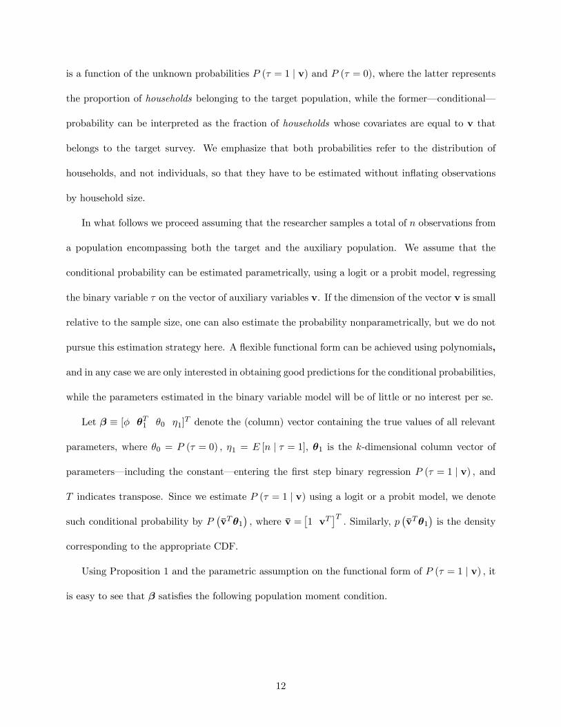
is a function of the unknown probabilities P (τ = 1 | v) and P (τ = 0), where the latter represents
the proportion of households belonging to the target population, while the former–conditional–
probability can be interpreted as the fraction of households whose covariates are equal to v that
belongs to the target survey. We emphasize that both probabilities refer to the distribution of
households, and not individuals, so that they have to be estimated without inflating observations
by household size.
In what follows we proceed assuming that the researcher samples a total of n observations from
a population encompassing both the target and the auxiliary population. We assume that the
conditional probability can be estimated parametrically, using a logit or a probit model, regressing
the binary variable τ on the vector of auxiliary variables v. If the dimension of the vector v is small
relative to the sample size, one can also estimate the probability nonparametrically, but we do not
pursue this estimation strategy here. A flexible functional form can be achieved using polynomials,
and in any case we are only interested in obtaining good predictions for the conditional probabilities,
while the parameters estimated in the binary variable model will be of little or no interest per se.
Let β ≡ [φ θT1 θ0 η1]T denote the (column) vector containing the true values of all relevant
parameters, where θ0 = P (τ = 0) , η1 = E [n | τ = 1], θ1 is the k-dimensional column vector of
parameters–including the constant–entering the first step binary regression P (τ = 1 | v) , and
T indicates transpose. Since we estimate P (τ = 1 | v) using a logit or a probit model, we denote
such conditional probability by P¡vTθ1
¢, where v =
£1 vT
¤T. Similarly, p
¡vTθ1
¢is the density
corresponding to the appropriate CDF.
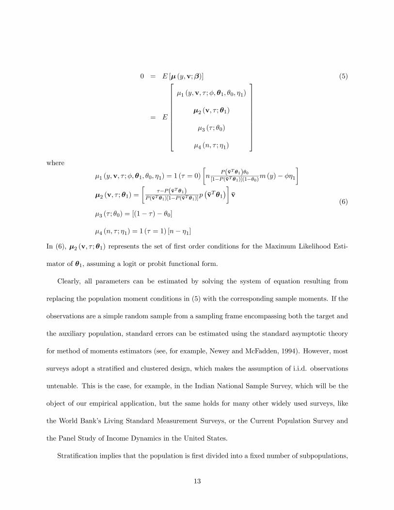
Using Proposition 1 and the parametric assumption on the functional form of P (τ = 1 | v) , it
is easy to see that β satisfies the following population moment condition.
12
0 = E [µ (y,v;β)] (5)
= E
µ1 (y,v, τ ;φ,θ1, θ0, η1)
µ2 (v, τ ;θ1)
µ3 (τ ; θ0)
µ4 (n, τ ; η1)
where
µ1 (y,v, τ ;φ,θ1, θ0, η1) = 1 (τ = 0)
·n
P(vT θ1)θ0[1−P (vT θ1)](1−θ0)m (y)− φη1
¸µ2 (v, τ ;θ1) =
·τ−P(vT θ1)
P (vT θ1)[1−P (vT θ1)]p¡vTθ1
¢¸v
µ3 (τ ; θ0) = [(1− τ)− θ0]
µ4 (n, τ ; η1) = 1 (τ = 1) [n− η1]
(6)
In (6), µ2 (v, τ ;θ1) represents the set of first order conditions for the Maximum Likelihood Esti-
mator of θ1, assuming a logit or probit functional form.
Clearly, all parameters can be estimated by solving the system of equation resulting from
replacing the population moment conditions in (5) with the corresponding sample moments. If the
observations are a simple random sample from a sampling frame encompassing both the target and
the auxiliary population, standard errors can be estimated using the standard asymptotic theory
for method of moments estimators (see, for example, Newey and McFadden, 1994). However, most
surveys adopt a stratified and clustered design, which makes the assumption of i.i.d. observations
untenable. This is the case, for example, in the Indian National Sample Survey, which will be the
object of our empirical application, but the same holds for many other widely used surveys, like
the World Bank’s Living Standard Measurement Surveys, or the Current Population Survey and
the Panel Study of Income Dynamics in the United States.
Stratification implies that the population is first divided into a fixed number of subpopulations,
13
called strata, which are usually defined following geographical and/or socioeconomic criteria. Then
a predetermined number of first stage units (households or clusters, see below) are sampled in-
dependently from each stratum. Stratification, then, typically reduces the standard errors of the
estimates, since all possible samples contain a fixed proportion of observations from each stratum.12
With clustering, instead, households are not sampled directly from the population (or from a stra-
tum), but are selected in a second stage from clusters, typically villages or urban blocks, which
are therefore the first stage units of the survey. Since households selected from the same clusters
tend to be relatively homogeneous, intra-cluster correlation is usually positive, which almost always
implies an increase in the standard errors of the estimates.13 In some surveys, including the NSS,
the design is further complicated by the presence of second-stage stratification, which is present
when each selected cluster is split into separate sub-clusters, and a fixed number of households is
selected from each subcluster.
Notice also that in most surveys the sampling scheme is such that households selected from
different clusters have a different ex-ante probability of being selected. This is the case, for example,
if clusters are selected via simple random sampling in the first stage, and a constant number of
households is sampled from each selected cluster in the second stage. This implies that, before
clusters are selected, households living in larger clusters have a smaller probability of being sampled.
So, unless clusters are selected with probability proportional to their size, consistent estimation of
population parameters requires the use of sampling weights, which ‘inflate’ each observation by the
inverse of the probability of selection.14
For all these reasons, here we use the results in Bhattacharya (2002), who studies the asymptotic12See Deaton (1997, Ch. 1) or Howes and Lanjouw (1995, 1998) for an introduction to the econometrics of stratified
and clustered samples.13On the other side, clustering allows the interviewers to visit a smaller number of locations, so reducing the cost
of the survey.14See Deaton (1997, Ch. 3) for a discussion of sampling weights.
14
properties of Method of Moments estimators allowing for the presence of two-stage stratification,
clustering, and sampling weights.
Suppose that the population is divided into S strata, and that stratum s contains a mass of Hs
clusters. Cluster c is further divided into Sc second-stage strata, each one containing M (s, c, sc)
households. Then, the population moment condition can be written as
0 =SXs=1
HsEc
ScXsc=1
M(s,c,σ)Xh=1
µ (yscsch,vscsch;β) | s (7)
where the expectation in curly brackets is taken with respect to the distribution of clusters in
stratum s, and β denotes the true value of the vector of parameters. If ns clusters are selected from
the sth stratum, and mscsc households are selected in the sc-th second-stage stratum in cluster c
belonging to stratum s, the sample equivalent of (7) is
0 =SXs=1
Hsns
nsXc=1
ScXsc=1
M (s, c, sc)
mscsc
mscscXh=1
µ³yscsch,vscsch; β
´(8)
where (nsmscsc)−1HsM (s, c, sc) represents the sampling weight.15
Bhattacharya (2002) obtains the asymptotic results letting the total number of selected clus-
ters–denoted by n–grow to infinity, while the number of households selected in every second-
stage stratum is kept constant, as well as the proportion of clusters selected per stratum, denoted
by as = ns/n. This is appropriate for our empirical application, since in the Indian NSS the total
number of clusters selected is much higher than the number of households selected per cluster.15 It is instructive to note that the expected value of the sum of the sample weights is an estimate of the total mass
of households in the population. In fact:
E
"SXs=1
nsXc=1
ScXsc=1
mscscXh=1
Hs
ns
M (s, c, sc)
mscsc
#
=SXs=1
HsE
"1
ns
nsXc=1
ScXsc=1
mscscXh=1
M (s, c, sc)
mscsc
| s#
=SXs=1
HsE
"ScXsc=1
M (s, c, sc) | s#
15
Besides complicating the notation, the presence of the complex survey design complicates the
asymptotics, since observations are now neither independent–since observations coming from the
same cluster are typically correlated–nor identically distributed, since observations are selected
from different strata, which are typically characterized by different distributions. However, Bhat-
tacharya (2002) notes that the clusters are independent, and so (8) can be rewritten as the average
of n independent terms. So, re-indexing clusters by i, we have
1
n
nXi=1
mi
³β´
= 0 where (9)
mi
³β´
=SXs=1
Hsas1 (i ∈ s)
SiXsi=1
M (s, i, si)
msisi
msisiXh=1
µ³ysisih,vsisih; β
´Then Bhattacharya (2002) identifies sufficient regularity conditions for consistency and asymptotic
normality, and shows that the following result holds:
√n³β − β0
´d→ N
³0,Γ−1W
¡Γ−1
¢T´(10)
where note that the asymptotic covariance matrix has a form analogous to the standard robust
variance allowing for arbitrary heteroskedasticity and group serial correlation. In the appendix we
describe the functional forms or Γ andW in our context, as well as their consistent estimators, and
we report–for the sake of completeness–the full proposition in Bhattacharya (2002).
Since we use observations sampled from two different databases, one has to be explicit about
how the sampling from the two populations is done. We consider the case where first stage strata are
the same across the two subpopulations, and we take the states to represent different strata.16 To
preserve independence across clusters, we maintain the assumption that, in each stratum, clusters
are selected randomly from a sampling frame encompassing both the target and the auxiliary16 In the NSS, strata are actually defined at a much finer level. Broadly, strata are districts in the rural sector
sectors, and town, or sections of large towns, in urban areas. In the NSS, allowing for stratification has typically
negligible effects on the standard errors, while allowing for clustering is important.
16
population.
4 An application to the estimation of Poverty in India
For decades, the Planning Commission of the Government of India has regularly published “official”
headcount poverty ratios, separately for rural and urban areas of every Indian state and Union
Territory. The poverty counts are computed as the fraction of the population living in households
in which total consumption per person is below the poverty line, which is kept constant over time
in real terms.17 The poverty lines are price-inflated using two different state-specific price indexes:
the Consumer Price Index for Agricultural Labourers (CPIAL) for rural areas, and the Consumer
Price Index for Industrial Workers (CPIIW) for the urban sector.18 Data on household expenditure
are collected by the Indian National Sample Survey Organization (NSSO) approximately every five
years, from a large sample of Indian households interviewed over a one-year period. Each NSS
round contains information on a wide spectrum of socioeconomic variables, but the largest section
of the database consists of records of household consumption of a very detailed list of items.19
17 In the early seventies, NSS expenditure data have also been used to estimate the calorie Engel curves the poverty
lines are based on. The lines have been computed to represent the total monthly per capita expenditure associated,
on average, with a sector-specific minimum calorie intake, as recommended by the Indian National Institute of
Nutrition. At the time of writing, official poverty estimates that use such lines are available for 1973-74 (28th NSS
Round), 1977-78 (32nd), 1983-84 (38th), 1987-88 (43rd), 1993-94 (50th), and 1999-2000 (55th).18These price indexes are available through a number of publications issued by the Government of India (for
example the Statistical Abstract). For a detailed overview of the issues related to the choice of poverty lines in India
see GOI, Planning Commission (1993), or Deaton and Tarozzi (2000), who also criticize the appropriateness of the
indexes used to price inflate the lines, and propose alternatives. For a different set of poverty lines, developed within
the World Bank, see also Datt (1999).19The item list is extremely detailed, and purportedly exhaustive. The questionnaire lists, for example, approxi-
mately 200 different food items.
17
Until the 50th round, carried out in 1993-94, all NSS surveys adopted a 30-day recall period
for all expenditure items. This choice of recall period is unusual, and most statistical agencies use
a much shorter recall period for items–like food–that are typically purchased frequently, and a
longer recall periods for infrequent expenditures like clothing, footwear, educational expenses, and
durables. Several experimental studies find that expenditure reports for frequently purchased items
are on average proportionally lower when the recall period becomes longer.20 According to some,
a switch to more standard recall periods would have helped reconciling the high rate of growth
measured by the National Accounts Statistics in the nineties, and the unimpressive rates of poverty
reduction estimated using NSS data over the same period. To explore further the issue, the NSSO
experimented with different recall periods using the smaller (‘thin’) NSS rounds that followed the
1993-94 survey. Such surveys were not specifically designed for poverty monitoring, so some doubts
remain on the comparability of their sampling frames, but each survey did also gather information
on expenditure on a list of items basically identical to the standard one.21 However, the NSSO
adopted two different expenditure questionnaires and only one of them was assigned at random to
all households living in a given primary stage unit of the survey. One questionnaire type–schedule
1–was the standard one, with a 30-day recall period for all items, while in the other type–schedule
2–the recall period was set equal to the 7 days before the interview for food, beverages and some
other items generally bought frequently, and to 365 days for durables, clothing, footwear and some20See, in particular, Scott and Amenuvegbe (1990). The 30-day recall period was adopted because of an early
experimental study by Mahalanobis and Sen (1954). This study does find a negative relation between reported
expenditure and length of the recall period, but finds that reports based on a 7-day recall period are too high. A new
study carried out by the NSSO (2003) suggests instead that the shorter recall period is more appropriate for many
high-frequency expenditures.21Most NSS rounds do not focus specifically on expenditure, and are carried out over a smaller sample than the
one typical of a ‘quinquennial’ round. For example, the main focus was on education and fertility in the 52nd round,
and on informal sector enterprises in the 51st.
18
other low-frequency purchases. For what follows, it should be kept in mind that the standard 30-
day recall period was instead kept in both schedules for a list of items accounting for a substantial
share of the budget. This list included fuel and light, miscellaneous goods and services, rents and
consumer taxes, and non-institutional medical expenses.22 We will generally refer to this list of
items as ‘30-day’ or ‘miscellaneous’ items.
The experimental surveys once again confirmed the finding that reported expenditure in food is
significantly higher if the recall period is shortened. The opposite result was found for most durables:
even if more households report some purchases when a one year recall period is adopted, average
monthly expenditure is lower than the one observed using a 30-day reference period.23 Given the
large average fraction of the budget spent in food, the net effect in all surveys and in both sectors is
a larger estimate of total per capita expenditure (pce) when the experimental questionnaire is used.
Table 1 contains summary statistics for the major Indian states.24 In all surveys and both sectors,
average total monthly pce is systematically 10-20 percent higher for households in the experimental
group, and the differences are always statistically significant at standard statistical levels. Row (5)
shows that, if one keeps the poverty line constant, this gap would translate into a fifty percent drop
in poverty ‘achieved’ through a change in the survey methodology.25 However, the results in row22The distinction between institutional and non-institutional medical expenses lies in whether the expenses were
incurred for medical treatment as an in-patient at a medical institution or otherwise.23For details, see Deaton (2001) and Sen (2000).24Such states include Andhra Pradesh, Assam, Bihar, Gujarat, Haryana (urban sector only), Jammu & Kashmir,
Karnataka, Kerala, Madhya Pradesh, Maharashtra, Orissa, Punjab, Rajasthan, Tamil Nadu, Uttar Pradesh, West
Bengal, and Delhi. These states account for more than 95 percent of the total Indian population.25The fact that the poverty lines are based on predicted calorie consumption given total pce might suggest that
if the revised questionnaire had to be used for poverty monitoring, the lines should be recalculated. Deaton (2001)
notes that doing so would, if anything, further increase the gap. Since a shorter recall period causes a larger
proportion of the reported total budget to be spent in food, then a lower level of pce would be necessary to achieve
the recommended minimum calorie intake. This would further reduce poverty. However, after analyzing the Engel
19
(3) show that the differences in reports on miscellaneous items are always very small, and in most
cases not statistically significant. This is crucial for our purposes, since it gives some preliminary
support to the claim that reports on a set of items are not influenced by reports in a different set
of items. This observation makes expenditure in miscellaneous items an excellent candidate for the
inclusion in the vector of auxiliary variables. Moreover, the figures in row (5) show that 30-day
items are likely to be good predictor of total pce, since the corresponding average budget share
is above 20 percent in the rural sector–using standard questionnaires–and above 25 percent in
urban areas. In each one of the surveys represented in Table 1, a simple log-linear regressions of
total pce on pce in 30-day expenditure produces an R2 above 0.65.
However, close examination of the figures in row (3) shows that in the rural sector mean pce
in miscellaneous items is systematically higher when computed using the standard questionnaire,
even if the differences are always small. The sign of the differences is reversed in the urban sector.
This empirical regularity is likely to be related to sectoral differences in consumption patterns and
in household characteristics. The cognitive processes adopted to remember expenditure should
be expected to be related to the item specificity, and to the characteristics of the respondent.
This suggests that it might be important to include household characteristics among the auxiliary
variables. Here we will make use of information on household size, completed education of the
household head, a categorical variable for land holdings, main economic activity of the household,
and whether the household belongs to special social groups (called ‘Scheduled Castes and Tribes’
in NSS). We will generally refer to these variables as (household-specific) controls.
Finally, notice that the figures in Table 1 show no apparent trend in poverty reduction over the
examined period. However, the thin rounds were not specifically designed as expenditure surveys.
The relatively small samples, coupled with the choice of sampling frames more suited to the different
curves for food, Deaton (2001) argues that the poverty lines should remain the same.
20
main purpose of these surveys, induced many observers to look at these poverty figures with some
suspicion, and to wait for the next quinquennial expenditure survey, that is, for the 55th round of
the NSS.
In the 55th round of the survey, the NSSO decided to adopt a questionnaire combining both sets
of recall periods used in the thin rounds. Expenditure in food was to be recorded using both the
30-day and the 7-day recall periods for all households, while for durables and other infrequently
purchased items only a 365-day recall period was to be used. The unadjusted results estimated
by the Indian Planning Commission showed an impressive reduction in poverty with respect to
the early nineties: using the data collected with a 30-day reports for food, in the rural sector the
counts dropped from 37.2 in 1993-94 to 27.1 six years later, while in urban areas the proportion
dropped from 32.6 percent to 23.6. In both cases this amounts to a reduction of one third in poverty
rates, in less than a decade. However, the changes in the questionnaire cast serious doubts on the
comparability of the more recent figures with previous poverty estimates, especially if one considers
the results of the thin experimental rounds.
On the one hand, the thin rounds showed that reports on durables are on average lower when
a 1-year recall period is used, so that the new questionnaire would overstate poverty. At the same
time, more respondents reported some expenditure in durables, with the consequence that the
corresponding distribution is much more spread out when the shorter recall period is used. Keeping
the average report constant, this would cause the opposite result of lower poverty estimates when
the experimental questionnaire is used. The two conflicting effects combine with the fact that
durables typically account for a small share of the total budget, especially among poor households,
making it unlikely that important comparability issues arise as a consequence.
On the other hand, the new questionnaire recorded the two separate reports on food expendi-
ture in two parallel columns printed next to each other. One can therefore expect that this format
21
prompted the respondents (or the interviewers) to reconcile the two different reports. So, consump-
tion of food reported with the traditional 30-day recall period would be disproportionately high
(since the respondent would tend to avoid large discrepancies with the 7-day reports, which are
typically higher), and/or the corresponding reports based on a 7-day recall period would be dispro-
portionately low (by a symmetric argument). The plausibility of this argument is strengthened by
the fact that in the 55th round average pce in food as estimated with a 7-day recall period exceeded
the corresponding figure calculated using the 30-day recall period by about 6 percent, while in
all the thin rounds the gap was consistently above 30 percent. Since for most Indian households
food accounts for a very large share of the total budget, these arguments lead to the expectation
that the unadjusted figures might significantly overstate total expenditure, and therefore signifi-
cantly understate poverty. Surprisingly, we find that our adjustment procedure does not change
considerably the poverty estimates, suggesting that the reconciliation between the sets of reports
on food expenditure worked mostly in one direction, shifting the 7-day reports downwards towards
the 30-day reports, but not vice versa.
4.1 Validating the Assumptions
In each thin round, every household received only one questionnaire type, so for each respondent
we observe either (y,v, τ) or (y, v,τ) . However, the questionnaire type was assigned randomly to
households, so that the distribution of both (y,v, τ) and (y, v,τ) are identified in each survey.
This fact can be used to provide support to the identifying assumptions needed for our adjusted
estimates to be reliable. In the rest of the paper, we will not use data from the 54th round. This
survey was carried out over a six-month period, while all other rounds are carried out over a whole
year, so seasonality issues might cause comparability problems.
Assumption A1 requires that the reports on the variables included in v be independent of the
22
questionnaire type. This assumption is easily tested for the discrete household specific controls
that we include in v, all of which are discrete. For each sector and survey we test the hypothesis
that the distribution of each of these variables is independent upon the questionnaire types, by
using a Pearson χ2 statistic modified to take into account stratification and clustering.26 Under the
null hypothesis, once we tabulate observations across values and schedules, the ‘joint’ proportion of
observations in the cell related to the the i-th value and the k-th schedule, should be the same as
the product of the ‘marginal’ proportion of observations having the i-th value, and the ‘marginal’
proportion of observations in the k-th schedule. The test rejects the null when a normalized sum
of the differences between joints and products of marginals is large. We report the p-values of
each test in Table 2. The results strongly support the null. Only 3 out of 30 tests reject the null,
and even in these cases the proportions are very similar across the schedules, as one can see from
the cross tabulations reported in the lower part of Table 2. These results are hardly surprising,
since the two different questionnaires are assigned randomly, and there is no obvious reason why
differences in the recall periods should affect respondents’ reports on the household controls we use
here.
Let m and m denote the (log of) pce in miscellaneous items, as measured respectively in a
standard and experimental questionnaire. Assumption A1 requires the equality of the densities of
m and m in the same round and sector. In Figure 1 we draw nonparametric kernel estimates of
the densities of m, m, y and y for each survey and sector.27 It is apparent that in all cases the
distribution of y is shifted to the right with respect to the distribution of y. This is consistent with
the results in Table 1, which showed that mean total pce is systematically higher for households in26More precisely, we use a second-order corrected Pearson statistic, as in Rao and Scott (1984). This test can be
performed using the “svytab” command in STATATM .27We use the robust bandwidth proposed by Silverman (1986) for the estimation of approximately normal densities
with a biweight kernel.
23
the experimental group. However, there is no such large and systematic gap between the distribu-
tions of m and m. Only in the urban sector of the 51st round does the difference between the two
curves appear visually not negligible, but even in this case the two densities closely coincide for low
values of expenditure, which is the relevant range when one is interested in poverty counts. We
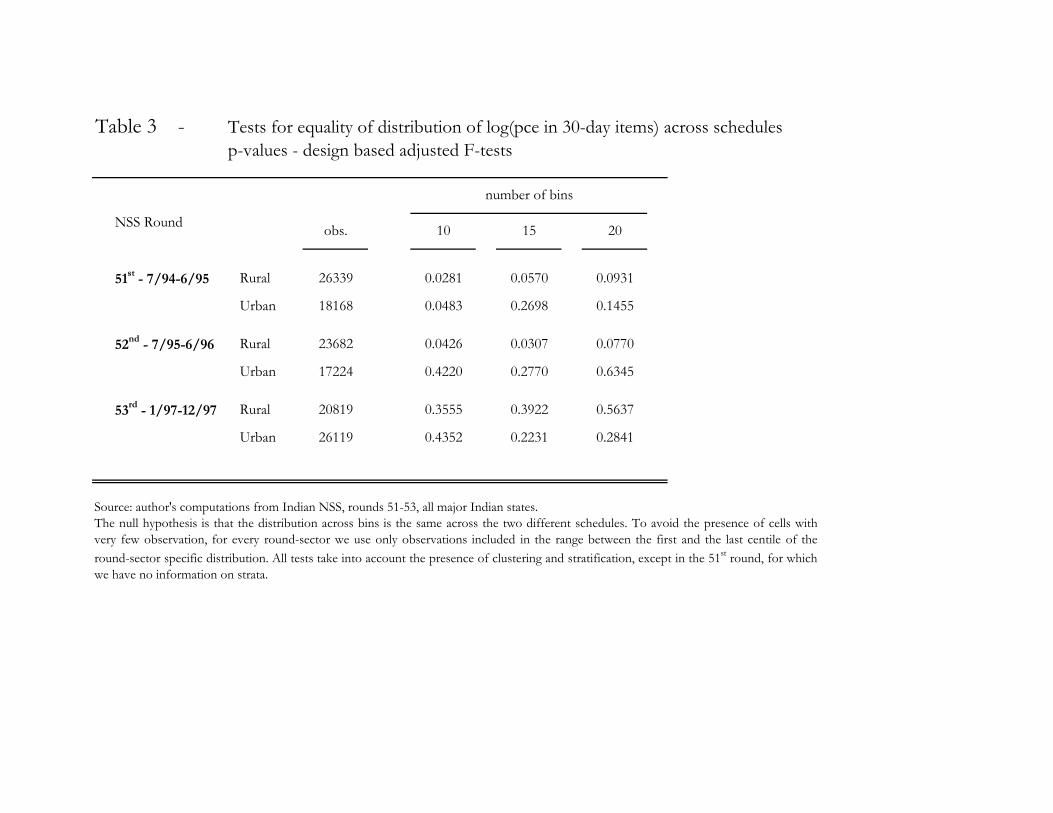
perform a simple test for the equality of the distributions of m and m using the Pearson χ2 statistic
described above.28 First we divide the range of m into bins of equal length, and then we test the
null hypothesis that the distribution of the observations across bins is independent upon the sched-
ule used to measure m. To avoid the presence of many empty cells, we consider only observations
included between the first and the last percentile of the round-sector distribution. Table 3 shows
the estimated p-values computed using 10, 15, or 20 bins, as a robustness check. In most cases the
null hypothesis cannot be rejected, and the p-values are above 0.2. The null is never rejected if we
use a one percent significance level, while using a five percent level we reject in the rural sector of
the 52nd Round, with 10 or 15 bins, and in both sectors of the 51st Round with 10 bins.
Overall, assumption A1 appears to hold well for the variables we plan to include in v, so
we move to analyze assumption A2, which in this context requires the stability over different
rounds of the probability of being poor, conditional on the observed v. In Figure 2 we plot the
estimated probabilities conditional onm only. Each line represents a nonparametric locally weighted
regression on m of a dummy variable equal to one when a household’s pce is below the poverty
line z.29 Because we are interested in the stability of P (y < z | m) , all the lines are constructed28We do not use a Kolmogorov-Smirnov test for the equality of two densities estimated nonparametrically since
this test does not allow for the presence of a complex survey design.29 In a locally weighted regression a “local” OLS regression is run at every point where the conditional expectation
is evaluated (see Fan, 1992). The regression is local since at every point we use only observations for which the
regressor is inside a neighborhood of the point itself, defined by a bandwidth. The observations are weighted by using
a kernel, so that observations closer to the point have more weight in the regression itself. We prefer locally weighted
regressions to the traditional Nadaraya-Watson estimators since the former tends to reduce the bias arising in the
24
using only observations from households that received the standard questionnaire. Even if the lines
do present some systematic gaps in some areas of their range, they look extremely similar overall,
suggesting that the assumption of a constant conditional probability is at the very least a sensible
working hypothesis. Note also that there is no apparent time trend in the way the curves differ
from each other, suggesting that no important gradual change is affecting the relation between m
and y.
In our context, the availability of empirical evidence supporting the stability of the conditional
probability is extremely important, since there are several reasons why such assumption might fail.
The major concern is that movements in the relative price of m should be expected to affect the
conditional probability of being poor, whose stability ultimately depends upon the stability of the
Engel curve linking y to m. Also, changes in tastes–or other demand shocks–might change the
relation between one survey and another. All these concerns are likely to be less pressing if the
auxiliary and the target survey are carried out in consecutive years. In any case, note that our
procedure is flexible enough to accommodate many of these factors, as long as they are observable,
and therefore can be included in the vector v.
As a further check, we impose a logit functional form to the conditional probability P (y < z | v) ,
and we test for the equality of the coefficients across surveys. In Table 4 we report robust tests for
the equality of coefficients across surveys for each pair of rounds, for the rural and urban sectors
separately, and using different sets of variables included in v. Over a total of 60 tests, the joint null
hypothesis of equal coefficients is rejected in 21 cases using a five percent significance level, and in
11 cases using a one percent level. Overall, the conditional probabilities appear remarkably stable,
especially taking into account the very large size of the samples (each tests uses a minimum of
estimates when the density of the regressor is not flat. For a clear treatment of the Nadaraya-Watson estimator see
Pagan and Ullah (1999, Ch. 3). Deaton (1997, Ch. 3) provides an intuitive treatment of locally weighted regressions.
25
18153 of observations, and a maximum of 72528), and the fact that in most cases the null imposes
more than twenty restrictions.
4.2 Performance of the Estimator
The previous section shows that the assumptions needed for the good performance of our adjustment
procedure are reasonable, in our empirical context. As a further check. we use the thin rounds
to perform an empirical exercise in order to evaluate the performance of the estimator. For each
thin round we can estimate a ‘comparable’ poverty count using data on total pce from the subset
of households who received a standard questionnaire. Then we can attempt to replicate these
‘benchmark’ poverty rates, using data on the auxiliary variables collected from households who
received an experimental questionnaire, while deriving information on P (y < z | v) from any of
the available standard surveys. Using the robust standard errors estimated using the procedure
described earlier in the paper, we test for the significance of the difference between the benchmark
and the adjusted poverty ratios. If the reweighting procedure performs well, one should not be able
to reject the hypothesis that the two estimates are equal.
We report the results of the tests in Table 5. Columns 1 and 2 report the benchmark and
the unadjusted poverty count for each round. As we already pointed out, the poverty counts are
approximately halved when the experimental surveys are used. In every case the differences are
statistically significant at any standard significance level. Columns 3 to 6 report the adjusted
poverty ratios and their standard errors, while asterisks denote the cases in which the null of no
difference between benchmark and adjusted ratios is rejected. Each test is simply based on the
ratio between the difference and its standard error. Since in each cell the benchmark and the
adjusted ratio are computed using data from independent surveys, such standard errors are trivial
to compute, once one has the standard errors for each poverty count. For each sector in each
26
thin round, ordered along the rows of the tables, we experiment using auxiliary data from the
same sector, in either the 50th round, or from the standard survey in each of the thin rounds. For
each target-auxiliary pair we use three different sets of auxiliary variables: a polynomial in m and
household size, a polynomial in household size and dummies for household controls, or all of the
above.
The results are mixed, but overall encouraging. Using a five percent significance level, the null is
not rejected in 48 out of 72 tests. The null is never rejected when we use the standard survey in a thin
round as auxiliary survey for the experimental survey in the same round. This can be interpreted
as further indirect evidence of the validity of assumption A1, since the random assignment of
questionnaire type should guarantee that, within the same round, assumption A2 holds. In all
cases, the absolute differences between the benchmark and the adjusted figures are much lower
than the differences across questionnaire types in the same round. However, in the rural sector,
when m is included among the auxiliary variables, the adjusted figures are systematically above
the corresponding benchmark, by 3-5 percentage points. However, this should not suggest that
excluding m from the auxiliary variables would improve the performance of the estimator. In fact,
careful examination of the adjusted estimates obtained excluding m reveals that the adjustment
does little more than reproducing the poverty ratio from the corresponding auxiliary survey. For
example, the headcount ratio for the rural sector of the 51st round is 41.8, and adjusted ratios
calculated using this as auxiliary survey are 41.6 in the 52nd round, and 40.9 in the 53rd round. If
the auxiliary survey is the 53rd round, in which the benchmark poverty ratio is 35.7, the adjusted
headcounts are 35.3 for the 51st round, and 35.6 for the 52nd round. One plausible explanation is
the fact that since the household controls do not explain a large fraction of the total variance of y, so
that the reweighting function R (v) is everywhere close to one, and as a consequence the adjustment
merely reproduces the poverty count in the auxiliary survey. For this reason, when applying our
27
adjustment procedure to the 55th NSS round, we always include m among the auxiliary variables.
As one would expect, there is a close correspondence between the performance of the estimator
and the results of the tests for the validity of the identifying assumptions that we described in
the previous sections. For example, in the urban sector of the 53rd round the hypothesis that the
benchmark and the adjusted ratios are the same is rejected in all specifications, when the 52nd
round is used as auxiliary survey. At the same time, the figures in the bottom panel of the last
column in Table 4 show that, for this pair of rounds, the assumption of equal conditional probability
in the same urban sector always fails. We observe the opposite if we use the 51st round as auxiliary
survey for the 53rd (or vice-versa). These results clearly stress that in empirical applications much
care should be taken in evaluating the credibility of the identifying assumptions.
4.3 Adjusted Poverty Estimates from the 55th Round of the National Sample
Survey
The questionnaire adopted in the 55th round of the NSS is different from any previously adopted
one. We already mentioned that the questionnaire asked all respondents to report consumption in
food using two different recall periods, while a 365-day recall period was introduced for consumption
on durables and some other items. However, expenditure in miscellaneous items, a good predictor
of total pce, was reported only using the standard 30-day recall period, so we can use this variable,
together with other controls, to implement our adjustment procedure. In the previous section we
provided indirect evidence supporting the stability of the conditional probability of being in poverty
given the auxiliary variables, and we showed that changes in some sections of the questionnaire
seem to have only mild consequences on reports recorded in unchanged sections.
Table 6 contains the sector-specific adjusted estimates for the poverty counts. As a robustness
check, we use all the NSS surveys between the 50th and the 53rd Round as auxiliary surveys. As
28
usual, we make use of the official poverty lines for all India in 93-94 Rupees. All monetary values
from subsequent Rounds are deflated using state and sector specific official Consumer Price Indexes.
Here we exclude Jammu and Kashmir from our estimates since we do not have information on the
relevant price indexes for the latest survey period. We report two sets of estimates. In Column 1 v
includes a cubic in m and household size. In Column 2 we also include the other household-specific
controls mentioned earlier in the paper. We obtain all adjusted poverty ratios using the expression
in (8), while the standard errors are computed as the first element along the diagonal of the robust
covariance matrix in (10).
The unadjusted poverty figures for the states included in our analysis are 28.4 percent in rural
areas and 24.5 percent in urban areas. In all cases but one, our adjustment procedure produces
higher estimates of poverty, as expected. The one exception is the point estimate for urban areas
when the 52nd round is used as auxiliary survey, and household specific controls are not included
among the auxiliary variables. In the rural sector, adjusted poverty counts range from 30.4 percent
to 32.5 percent. In urban areas, the adjusted figures range from 24 to 27.3 percent. In all cases the
increase in point estimates is more pronounced if the controls are included. The inclusion of such
controls also slightly increases the estimated standard deviations.
Expenditure data from the previous quinquennial round, carried out in 1993-94, showed that
the proportion of the population in poverty in the states considered here was 33.4 percent in urban
areas, and 38.2 percent in the countryside. So, even if the adjustment delivers–as expected–
higher headcount ratios than the official ones, our estimates confirm a very large poverty reduction
in India during the nineties. This conclusion is consistent with the results obtained by Deaton
(2003b) and Sundaram and Tendulkar (2003). The latter authors, together with Deaton and Drèze
(2002), also argue that such large decline in poverty is consistent with evidence from employment
surveys, the National Accounts and from data on agricultural wages. So, our conclusion is that
29
most of the poverty reduction measured by using NSS data is real, and not simply a statistical
artifact due to a change in the survey design.
The relatively small difference between adjusted and unadjusted estimates suggests that most of
the reconciliation between 7-day and 30-day reports comes from a bias of the 7-day reports towards
the 30-day ones, and not vice versa.
5 Caveats and Conclusions
In this paper we introduce an intuitive and easily implemented method to compute comparable
statistics for differently designed surveys, when the different design causes the respondents’ reports
to be incomparable across the surveys. Our emphasis is in the estimation of poverty headcount
ratios, but the framework can be generally applied to a broad set of parameters satisfying a pop-
ulation moment condition of the form E [m (y)− φ] = 0, where y is the variable measured in a
non-comparable way in the different surveys. The procedure we propose requires the existence of a
set of auxiliary variables whose reports are not affected by the different survey design, and whose
relation with the main variable of interest is stable across the surveys.
The reliability of the adjusted estimates depends crucially on the reliability of the necessary
identifying assumptions, which should be carefully evaluated by the researcher on a case by case
basis. With this caveat, the procedure introduced here should be a very useful tool for the researcher
interested in the evolution over time of welfare or aggregate economic indicators, since changes in
survey methodology are frequent, and can easily lead to non-comparability issues.
We estimate adjusted poverty counts from the 55th round of the Indian National Sample Survey,
a large expenditure survey carried out in 1999-2000, for which comparability issues arose due to
changes in the adopted questionnaire. The identifying assumptions needed for the good performance
30
of our estimator involve unobserved variables, and therefore cannot be directly tested. However,
by using previous NSS rounds, we provide indirect evidence supporting to a large extent their
validity. According to our estimates, poverty counts in India in 1999-2000 were close to 30 percent
in rural areas, and 25 percent in urban areas. Even if these figures are slightly higher than the
unadjusted ones, they still show an impressive poverty decline in the nineties, since the previous
estimates–from the 1993-94 round of the NSS–were approximately 30 percent higher.
Even if our emphasis on comparability issues over time is justified by the empirical application,
the approach developed here also has other potentially fruitful applications. For example, one
can merge information on auxiliary variables from a census (which commonly does not record
expenditure) with data on the same variables and expenditure from a household survey, to recover
welfare measures for geographically small areas, for which a representative sample from the survey
is typically not available.30 More generally, the estimator can be used to mitigate the problem of
missing data, when the statistic of interest satisfies the moment condition described above, and
when data on an adequate set of auxiliary variables are available. Clearly, in every application the
plausibility of the identification assumptions should be carefully scrutinized.
The identifying assumptions will typically not hold if the target and the auxiliary surveys refer
to very different populations, so, for example, our methodology is unlikely to be useful if one needs
to make cross-country comparisons of welfare indicators.
As a final caveat, it should be stressed that in our empirical application we do not suggest the
superiority of one set of recall period over the others. Our scope is to ensure comparability over
time for otherwise incomparable statistics, but our methodology should not be interpreted as a
tool to solve a measurement error problem. In fact, even when the adjustment works perfectly,30For a different approach, see Elbers, Lanjouw and Lanjouw (2003), whose procedure explicitely focuses on the
estimation of micro-level poverty and inequality measures.
31
the adjusted estimates will not recover the true value of the parameter of interest. Rather, the
estimator aims at recovering the estimate for such parameter that one would have obtained if the
questionnaire change did not take place.
32
References
[1] Bhattacharya, Debopam, 2002, “Inference from multi-stage samples: asymptotic theory with
applications to poverty and inequality estimation”, mimeo, Princeton.
[2] Case, Anne, and Angus S. Deaton, 2002, “Consumption, health, gender, and poverty”, Re-
search Program in Development Studies, Princeton University, processed.
[3] Datt, Gaurav, 1999, “Has poverty declined since economic reforms?”, Economic and Political
Weekly, December 11, 3516—18.
[4] Datt, Gaurav, Martin Ravallion, and Valerie Kozel, 2003, “A model based assessment on
India’s progress in reducing poverty in the 1990s”, Economic and Political Weekly, January
25, 355-361.
[5] Deaton, Angus S., 1997, The analysis of household surveys: a microeconometric approach to
development policy, Baltimore, MD, Johns Hopkins University Press.
[6] Deaton, Angus S., 2001, “Survey design and poverty monitoring in India”, Research Program
in Development Studies, Princeton University, processed.
[7] Deaton, Angus S., 2003a, “Prices and poverty in India, 1987-2000”, Economic and Political
Weekly, January 25, 362-368.
[8] Deaton, Angus S., 2003b, “Adjusted Indian poverty estimates for 1999-2000”, Economic and
Political Weekly, January 25, 322-326.
[9] Deaton, Angus S., and Jean Drèze, 2002, “Poverty and inequality in India, a re-examination”,
Economic and Political Weekly, September 7, 3729-3748.
[10] Deaton, Angus S., and Margaret Grosh, 2000, “Consumption,” Chapter 5 in Margaret Grosh
and Paul Glewwe, eds., Designing household survey questionnaires for developing countries:
lessons from 15 years of the Living Standards Measurement Study, Oxford University Press for
the World Bank, Vol 1., 91—133.
[11] Deaton, Angus S., and Alessandro Tarozzi, 2000, “Prices and poverty in India,” Research
Program in Development Studies Working Paper no. 196, Princeton University.
[12] Di Nardo, John, Nicole M. Fortin, and Thomas Lemieux, 1996, “Labor Market Institutions
and the Distribution of Wages, 1973-1992: a Semiparametric Approach”, Econometrica, 64(5),
1001-1044.
[13] Elbers, Chris, Jean O. Lanjouw, and Peter Lanjouw, “Micro-level estimation of poverty and
inequality”, Econometrica, 71(1), 355-364.
[14] Fan, Jianquing, 1992, “Design-adaptive Nonparametric Regression”, Journal of the American
Statistical Association, 87, 998-1004.
[15] Ghose and Bhattacharya, 1995, “Effects of Reference Period on Engel Elasticities of Clothing
and Other Items: Further Results”, The Indian Journal of Statistics, 57, series B, 3, 433-449.
[16] Gibson, John, 1999, “How Robust are Poverty Comparisons to Changes in Household Survey
Methods? A Test Using Papua New Guinea Data”, Department of Economics, University of
Waikato.
[17] Gibson, John, 2002, “Why Does the Engel Method Work? Food Demand, Economies of Size,
and Household Survey Methods”, Oxford Bulletin of Economics and Statistics, 64(4), 341-359.
[18] Gibson, John, Jikun Huang and Scott Rozelle, 2001, “Why is income inequality so low in China
compared to other countries? The effect of household survey methods”, Economics Letters,
71(3), 329-333.
[19] Gibson, John, Jikun Huang and Scott Rozelle, 2003, “Improving estimates of inequality and
poverty from urban China’s Household Income and Expenditure Survey”, Review of Income
and Wealth, forthcoming.
[20] Government of India, 1993, Report of the Expert Group on the estimation of proportion and
number of poor, Delhi, Planning Commission.
[21] Government of India, various years, Statistical abstract, Delhi, Central Statistical Organization,
Department of Statistics, Ministry of Planning.
[22] Heckman, J., Lalonde, R., and Smith, J., 1999, “The Economics and Econometrics of Active
Labor Market Programs,” Handbook of Labor Economics, Volume 3A, Ashenfelter, A. and D.
Card, eds., Amsterdam: Elsevier Science.
[23] Horowitz, Joel L., and Charles F. Manski, 1995, “Identification and Robustness with Conta-
minated and Corrupted Data”, Econometrica, 63(2), 281-302.
[24] Howes, Stephen, and Jean Olson Lanjouw, 1998, “Does Sample Design Matter for Poverty
Rate Comparisons?, Review of Income and Wealth, Series 44, no. 1.
[25] Howes, Stephen, and Jean Olson Lanjouw, 1995, “Making Poverty Comparisons Taking Into
Account Survey Design: How and Why”, Policy Research Department, World Bank, Wash-
ington, D.C., and Yale University, New Haven, processed.
[26] Jolliffe, Dean, 2001, “Measuring absolute and relative poverty: the sensitivity of estimated
household consumption to survey design”, Journal of Economic and Social Measurement, 27,
1-23.
[27] Lanjouw, Jean Olson, and Peter Lanjouw, 2001, “How to Compare Apples and Oranges:
Poverty Measurement based on Different Definition of Consumption”, Review of Income and
Wealth, 47 (1), pp. 25-42.
[28] Mahalanobis, P. C., and S. B. Sen, 1954, “On some aspects of the Indian National Sample
Survey,” Bulletin of the International Statistical Institute, Vol. 34, part II.
[29] National Sample Survey Organization, 2003, “Stability of different recall period for measuring
household consumption: results of a pilot study”, Economic and Political Weekly, January 25,
307-321.
[30] Newey, Whitney, and Daniel McFadden, 1994, “Large Sample Estimation and Hypothesis
Testing”, in Handbook of Econometrics, Volume IV, R.F. Engle and D.L. McFadden eds.,
Elsevier.
[31] Pagan, Adrian, and Aman Ullah, 1999, Nonparametric Econometrics, Cambridge, Cambridge
University Press.
[32] Ravallion, Martin, 1993, Poverty Comparisons: a Guide to Concepts and Methods, LSMS
Working Paper 88, Washington, D.C., World Bank.
[33] Rao J. N. K., and A. J. Scott, 1984, “On chi-squared tests for multiway contingency tables
with cell proportions estimated from survey data”, Annals of Statistics, 12, 46-60.
[34] Sachs, Jeffrey D., Ashutosh Varshney, and Nirupam Bajpai, 1999, India in the Era of Economic
Reforms, Oxford, Oxford University Press.
[35] Scott, Chris, and Ben Amenuvegbe, 1990, “Effects of Recall Duration on Reporting of House-
hold Expenditures: An Experimental Study in Ghana”, Social Dimentions of Adjustment in
Sub-Saharan Africa Working Paper No. 6, Washington, DC, The World Bank.
[36] Sen, Abhijit, 2000, “Estimates of Consumer Expenditure and Its Distribution: Statistical
Priorities after NSS 55th Round”, Economic and Political Weekly, December 16, 2000, 4499-
4518.
[37] Silverman, Bernard W., 1986, Density Estimation for Statistics and Data Analysis, London,
Chapman and Hall.
[38] Sundaram, K and Suresh Tendulkar, 2002, “Recent Debates on Data Base for Mea-
surement of Poverty in India”, Delhi School of Economics, processed. Available at
http://www.worldbank.org/indiapovertyworkshop.
[39] Sundaram, K and Suresh D Tendulkar, 2003, “Poverty Has Declined in the 1990s: A Resolution
of Comparability Problems of NSS on Consumer Expenditure”, Economic and Political Weekly,
January 25, 322-326.
[40] Visaria, Pravin, 2000, “Poverty in India during 1994—98: alternative estimates,” Institute for
Economic Growth, New Delhi, processed.
Appendix
Proof of Proposition 1:
Using the law of iterated expectations, and A2, we can rewrite the initial moment condition as
Figure 1 - Source: author’s computation from NSS - All major Indian states. In each graph the two rightmost linesrepresent kernel estimates of the densities of total pce as measured with the two different schedules. The other two linesrepresent kernel estimates of the densities of pce in 30-day items. All values are in 1993-94 Rupees, deflated using CPIALfor the rural sector, and CPIIW for the urban sector. All densities are estimated using Silverman’s robust bandwidth adaptedfor a biweight kernel, which is the one we use here.
Figure 2 - Conditional probability of being poor given log(PCE in 30-day items) Source: author=s computations from NSS, rounds 50-53, all major Indian States. Locally weighted regressions. The dependent variable is a dummy variable equal to one when the household=s per capita monthly expenditure is below the sector-specific poverty line. The bandwidth used in each line is indicated in the corresponding label.
Deflator is CPIIW for urban sector and CPIAL for rural sector
Table 1 - Summary statistics, Indian NSS Rounds 51-54
rural urban
NSS 51
July 1994 - June 1995
rural urban rural urban
NSS 52
July 1995 - June 1996
NSS 54
January-June 1998
rural urban
Source: author's computations from NSS. Robust standard errors in parenthesis. All values in 1993-94 Rupees. Only the major Indian states are included. All statistics are weighted using inflation factors. S1 is the standard questionnaire, with a 30-day reference period for all items. S2 is the experimental questionnaire, with a 7-day recall period for food and other high frequency items, and a 365day recall period for durables, clothing, footwear, educational and institutional medical expenses. The category "30-day items" includes: fuel and light, miscellaneous consumer goods and services, rents, consumer taxes and non-institutional medical expenses. The mean budget shares are averages of household-specific ratios between expenditure in 30-day items and total expenditure. The poverty counts are the proportion of individuals living in households where per capita expenditure is below the poverty line. The poverty lines are the official ones published by the Planning Commission for 1993-94, and are expressed in 1993-94 Rupees (the exchange rate at the time was approximately (1US$/32 Rs). The poverty line for All India is Rs 205.7 for the rural sector, and Rs 283.4 for the urban sector.
2.73 7.464.919.573.07
0.561.342.462.100.480.182.09 0.62
2.4612.376.92
Table 2 – Tests for equality of distributions across schedules
Source: author's computations from Indian NSS, rounds 51-53. All major Indian states.The figures in panel (1) are p-values for Pearson chi-squared statistics corrected for the survey design. The null hypothesis is that, for every sector-roundpair, the distribution of the selected variable is the same across the two different schedules. "Education of head" is one of the following: illiterate, literatewith no schooling, literate below primary, primary, middle, secondary, above secondary. In the rural sector "Main activity of the household" is one of thefollowing: self-employed in non-agriculture, agricultural labor, other labor, self-employed in agriculture and others; in the urban sector the categories are:self-employed, regular wage/salaried, casual labor, others. "Land holdings" are recorded as a categorical variable, with different codes for different intervals:code 1 is for land holdings below 0.01 acres, code 2 for the interval [0.01,0.2) and so on.
NSS 51, Rural NSS 53, Rural NSS 53, Rural
51st round 52nd round 53rd round
Self-empl. in agr. and others
self-employed in non-agricultureagricultural laborother labor
Table 3 - Tests for equality of distribution of log(pce in 30-day items) across schedulesp-values - design based adjusted F-tests
Source: author's computations from Indian NSS, rounds 51-53, all major Indian states.The null hypothesis is that the distribution across bins is the same across the two different schedules. To avoid the presence of cells withvery few observation, for every round-sector we use only observations included in the range between the first and the last centile of theround-sector specific distribution. All tests take into account the presence of clustering and stratification, except in the 51st round, for whichwe have no information on strata.
number of bins
obs. 10 15 20
Table 4 - Tests for equality of conditional probabilities of being poor across different surveys
Polynomial in m and h. size, controls χ2(27) 32.54 38.66 39.38 31.09 28.31 45.49[0.2127] [0.0680] [0.0585] [0.2675] [0.3952] [0.0144]
Source: author's computations from NSS, rounds 50-53. Major Indian states only. The tests are robust to the presence of arbitrary heteroskedasticity and correlation within clusters. P-values in parenthesis. a m is (log) per capita expenditure in miscellaneous items, in 93-94 Rsb The controls are categorical variables for education of the household head, main economic activity of the household, whether the household belongs to a "scheduled caste or tribe", and land ownership.
Rural Sector
Urban Sector
(1) (2) (3) (4) (5) (6)
H1 H2 50 51 - Sch. 1 52 - Sch. 1 53 - Sch. 1
NSS 51 - 94/95 Rural 41.8 22.7 m only 46.4 (2.83)** 45.6 (1.70) 45.3 (1.77) 44.6 (1.22)s.e. (1.42) (1.19) all except m 38.0 (2.55)** 41.7 (0.13) 37.8 (2.31)* 35.3 (3.42)**
all 45.5 (2.27)* 45.3 (1.55) 45.0 (1.65) 43.9 (0.9)
Urban 36.3 18.5 m only 36.8 (0.27) 33.8 (0.94) 33.4 (1.33) 36.1 (0.06)s.e. (1.88) (1.34) all except m 33.4 (1.37) 36.6 (0.14) 32.0 (2.04)* 35.0 (0.56)
all 36.4 (0.08) 34.7 (0.6) 34.6 (0.77) 36.8 (0.28)
NSS 52 - 95/96 Rural 38.2 18.4 m only 41.7 (3.43)** 41.0 (1.70) 39.7 (1.31) 39.9 (1.06)s.e. (0.89) (0.74) all except m 38.4 (0.23) 41.6 (2.04)* 37.9 (0.16) 35.6 (1.63)
all 41.7 (3.42)** 41.2 (1.8) 40.4 (1.67) 39.8 (1.02)
Urban 30.7 15.4 m only 33.0 (2.27)* 30.7 (0.01) 30.4 (0.22) 33.3 (2.19)*s.e. (0.83) (0.69) all except m 32.0 (1.31) 35.5 (2.6)** 30.7 (0.01) 33.8 (2.64)**
all 32.6 (1.88) 31.2 (0.31) 30.8 (0.14) 33.6 (2.46)**
NSS 53 - 97 Rural 35.7 21.1 m only 40.1 (3.22)** 39.4 (2.06)* 39.0 (2.12)* 38.3 (1.53)s.e. (1.27) (1.06) all except m 37.3 (1.3) 40.9 (2.77)** 37.0 (0.95) 34.9 (0.34)
all 39.9 (3.09)** 39.7 (2.19)* 39.0 (2.1)* 38.4 (1.57)
Urban 33.1 17.5 m only 32.5 (0.90) 30.3 (1.88) 30.1 (3.01)** 32.9 (0.46)s.e. (0.83) (0.75) all except m 31.8 (1.61) 35.1 (0.87) 30.3 (2.8)** 33.9 (0.33)
all 32.1 (1.3) 30.7 (1.62) 30.3 (2.86)** 33.3 (0.14)
Source: author's calculations from NSS rounds 50-53. Only major Indian states are included. Columns 1 and 2 report robust standard errors in parenthesis. Columns 3 to 6 report in parenthesis the robust t-ratio for the null that the adjusted poverty ratio and the benchmark are the same. ** indicates rejection using 1% significant level, while * indicates rejection using 5% level.
Tar
get
surv
ey (S
ch. 2
)
a m is (log) per capita expenditure in miscellaneous items, in 93-94 Rsb The controls are categorical variables for education of the household head, main economic activity of the household, whether the household belongs to a "scheduled caste or tribe",and land ownership.
Table 5 - Adjusted and unadjusted poverty rates in thin rounds using a logit first step
Unadjusted Poverty Counts, only larger Indian States, Standard QuestionnaireRural 28.4 (0.40), Urban 24.5 (0.58)
The poverty lines are the official ones for the 50th round (205.67 for the rural sector, and 283.44 for the urban sector). Allmonetary values from subsequent Rounds are deflated using state and sector specific official Consumer Price Indexes (CPIALfor households living in rural areas, and CPIIW for those living in urban areas). All estimates are computed for all major Indianstates: Andhra Pradesh, Assam, Bihar, Gujarat, Haryana (urban only), Karnataka, Kerala, Madhya Pradesh, Maharashtra, Orissa,Punjab, Rajasthan, Tamil Nadu, Uttar Pradesh, West Bengal, Delhi (urban only). The adjusted poverty counts are estimates usingthe estimator developed in the paper, using a logit first step. In both columns, the logit first step also includes a polynomial inhousehold size.
Source: author's computation from NSS, Rounds 50-51-52-53-55. Robust standard errors in parenthesis.
a m is (log) per capita expenditure in miscellaneous items, in 93-94 Rsb The controls are categorical variables for education of the household head, main economic activity of the household, whetherthe household belongs to a "scheduled caste or tribe", and land ownership.