COMMUNICATIONS ON doi:10.3934/cpaa.2011.10.PURE AND APPLIED ANALYSISVolume 10, Number 5, September 2011 pp. –

A PARTICLE METHOD AND NUMERICAL STUDY OF A

QUASILINEAR PARTIAL DIFFERENTIAL EQUATION

Roberto Camassa

Department of MathematicsUniversity of North Carolina at Chapel Hill

Chapel Hill, NC 27599-3250, USA

Pao-Hsiung Chiu1, Long Lee2, and Tony W.-H. Sheu3

1Nuclear Engineering Division

Institute of Nuclear Energy Research

Taoyuan County, 32546, Taiwan (R.O.C.)

2Department of MathematicsUniversity of Wyoming

Laramie, WY 82071-3036, USA

3Department of Engineering Science and Ocean Engineering

National Taiwan UniversityTaipei City 106, Taiwan (R.O.C.)

(Communicated by ???)

Abstract. We present a particle method for studying a quasilinear partial dif-

ferential equation (PDE) in a class proposed for the regularization of the Hopf

(inviscid Burger) equation via nonlinear dispersion-like terms. These are ob-tained in an advection equation by coupling the advecting field to the advected

one through a Helmholtz operator. Solutions of this PDE are “regularized” in

the sense that the additional terms generated by the coupling prevent solutionmultivaluedness from occurring. We propose a particle algorithm to solve the

quasilinear PDE. “Particles” in this algorithm travel along characteristic curves

of the equation, and their positions and momenta determine the solution of thePDE. The algorithm follows the particle trajectories by integrating a pair of

integro-differential equations that govern the evolution of particle positions and

momenta. We introduce a fast summation algorithm that reduces the compu-tational cost from O(N2) to O(N), where N is the number of particles, andillustrate the relation between dynamics of the momentum-like characteristicvariable and the behavior of the solution of the PDE.

1. Introduction. Consider the quasilinear partial differential equation (PDE)

mt + umx = 0, m = u− α2uxx, α > 0. (1)

We refer to the above equation as the Helmholtz-regularized Hopf equation. Theequation is the b = 0 member of the b-family

mt + umx + b uxm = 0, m = u− α2uxx, α > 0, (2)

described in [7]. The present paper will focus only on equation (1), the b = 0 case.

2000 Mathematics Subject Classification. Primary: 65M25; Secondary: 35G25.Key words and phrases. Quasilinear partial differential equation, particle method, Helmholtz

operator, regularization, inviscid Burgers, Hopf equation.

1

2 ROBERTO CAMASSA, PAO-HSIUNG CHIU, LONG LEE AND TONY W.-H. SHEU

With the definition of the one dimensional Helmholtz operator as

H = 1− α2∂xx, (3)

and its Green’s function, one can represent the solution of equation (1) u in termsof m as

u(x, t) =1

2α

∫ ∞−∞

e−|x−y|/αm(y, t)dy. (4)

The Leray-type [10] smoothed velocity u has been recently proposed for its role ofregularizing the inviscid Burgers (Hopf) equation.

ut + uux = 0. (5)

With nonzero viscosity, the Burgers equation

ut + uux = νuxx (6)

is the simplest model combing the nonlinear propagation effect and the diffusiveeffect, while its inviscid version for ν = 0, also known as Hopf equation, is thesimplest model of shock forming hyperbolic equation. In [11, 12], attempts weremade to compare regularization effects induced by the viscosity and the filteredvelocity (4).

It is well-known that one can study the Burgers equation to determine the physi-cally relevant solutions of the Hopf equation. The regularized Burgers equation (1),written in the form

ut + uux = α2 (uxxt + uuxxx) , (7)

is a quasilinear equation that consists of the Hopf equation plus O(α2) nonlinearterms. An approach, similar to that for the Burgers equation, is proposed (see,e.g., [1]) to show that solutions of this equation converge strongly to physicallyrelevant weak solutions of the Hopf equation (5) as α→ 0, provided the initial datau(0, x) are in a suitable function space. Thus, equation (7) has been proposed as analternative to Burgers equation (5) in this respect. Part of the interest in studyingthis particular class of regularizations stems from the fact that, unlike its Burgercounterpart, it can be endowed with interesting mathematical structures [7] sharedwith the rest of the family (2).

It is worth noting that in the absence of either of the two terms on the righthand site of (7), the equation becomes

ut + uux = α2uuxxx, (8)

orut + uux = α2uxxt . (9)

Both of these are dispersive equations (as linearization around a constant solutionreadily shows) and have zero-dispersion limits. One can expect that high-frequencyoscillation will occur when α is small. However, when the two third derivative terms,uuxxx and uxxt, appear together in equation (7), the delicate balance between thetwo terms will cancel the high-frequency oscillation expected to arise in passing tothe zero-dispersion limits. For most numerical schemes, certain care is required todiscretize the two third-order terms in order to achieve a higher-order accuracy,while maintaining the delicate balance of the two terms. A dispersion-relation-preserving scheme is developed in [6] that maintains the balance between the twodispersive terms and is suitable to study the long-time solution behavior of equation(7). The study in this paper, however, takes a different route by developing a particlemethod that avoids any discretization of the spatial derivative terms in equation

PARTICLE METHOD AND HELMHOLTZ REGULARIZATION 3

(7). “Particles” in this algorithm travel along characteristic curves of the equation,and their positions and momenta determine the solution of the PDE. The algorithmfollows the particle trajectories by integrating a pair of integro-differential equationsthat govern the evolution of particle positions and momenta. The particle methodis a self-adaptive algorithm, since particles normally cluster in areas with sharpgradients. The particle method reveals dynamics of particle position and momenta,which sheds light on solution behaviors of the PDE we study. Such a special featuredistinguishes the particle method from Eulerian methods.

The rest of the paper is organized as follows. In Section 2, we define the char-acteristic variables and derive the evolution (integro-differential) equations for thecharacteristic variables. We introduce a finite dimensional particle system in Section3 by discretizing the integro-differential equations. We derive an implicit analyticsolution for a special case of two-particle dynamics, the particle-antiparticle colli-sion, which, although very simple, is remarkably informative on the trend of PDEsolutions with more general initial conditions. We verify the particle method in Sec-tion 4 by comparing the numerical solution of the particle-antiparticle collision withthe implicit exact solution. Then we present an example with an initial conditionthat is a Gaussian hump. We introduce a fast summation algorithm that reducesthe computational cost from O(N2) to O(N), where N is the number of particles.Using these more general initial data, we verify the proposed method by comparingour numerical solution with the solution computed by a two-step iterative method.Finally, we illustrate the relation between dynamics of the momentum-like charac-teristic variable and solution behaviors of the PDE.

2. Characteristic variables. In this section we introduce a particle method forthe regularized Burgers equation (1) following the one proposed in [3] (and studiedextensively in, e.g., [4, 5, 6, 8, 9]) for a shallow water equation that shares a similarstructure. By introducing the characteristics variable (curve)

x = q(ξ, t), q(ξ, 0) = ξ, (10)

equation (1) is equivalent to

dm

dt= m = 0, q = u(q, t), (11)

where the material (total) derivative is defined as

d

dt=

∂

∂t+ u

∂

∂x. (12)

Equation (11) suggests that the variable m is a constant along the characteristiccurve, or

m(q, t) = m0(ξ). (13)

Equations (11) and (4) imply that

q =1

2α

∫ ∞−∞

e−|q(ξ,t)−q(η,t)|/αm0(η)qη(η, t)dη. (14)

Defining an auxiliary variable

p(η, t) ≡ m0(η)qη(η, t), (15)

4 ROBERTO CAMASSA, PAO-HSIUNG CHIU, LONG LEE AND TONY W.-H. SHEU

taking a time derivative about the above equation, and using equation (14) yieldsthe evolution equation

p = − 1

2α2

∫ ∞−∞

sgn(q(ξ, t)− q(η, t))e−|q(ξ,t)−q(η,t)|/α

m0(ξ)qξ(ξ, t)m0(η)qη(η, t)dη.

(16)

Equations (14), (15), and (16) yield a pair of continuous evolution equations for pand q:

q(ξ, t) =1

2α

∫ ∞−∞

e−|q(ξ,t)−q(η,t)|/αp(η, t)dη,

p(ξ, t) = − 1

2α2

∫ ∞−∞

sgn(q(ξ, t)− q(η, t))e−|q(ξ,t)−q(η,t)|/αp(ξ, t)p(η, t)dη.(17)

After solving the above evolution equation, solutions of the PDE (1) u are found by

u(x, t) =1

2α

∫ ∞−∞

e−|x−q(η,t)|/αp(η, t)dη. (18)

Here the characteristic q(ξ, t) plays the role of positions conjugate to the momentum-like variable p(ξ, t). The initial conditions for p(ξ, t) and q(ξ, t) are

q(ξ, 0) = ξ, p(ξ, 0) = m0(ξ). (19)

The choice of initial condition for the position variable, dictated by the character-istics condition, implies qξ(ξ, 0) = 1, so that the constraint, obtained from equation(15),

qξ(ξ, t) =p(ξ, t)

p(ξ, 0), (20)

is maintained at all times of existence of the solution (q(ξ, t), p(ξ, t)). Thus, the mo-mentum variable p(ξ, t) could be eliminated from the system to obtain an evolutionequation containing only the dependent variable q(ξ, t) and its first derivative withrespect to the initial label ξ. Vanishing of this derivative generically correspondsto crossing of characteristics curves, with loss of uniqueness of solutions ξ(x, ·) tothe equation x = q(ξ, ·) that defines the characteristic map. Constraint (20) canthen be used to show that if the initial condition p(ξ, 0) is bounded, then qξ(·, t) isbounded away from zero, thereby preventing characteristics from crossing, as longas p(·, t) does not have zeros.

We argue, by contradiction, that for a finite ξ the derivative qξ cannot vanishin any finite time, provided the initial data p(ξ, 0) 6= 0. Suppose that t = T is thefirst time when crossing of characteristics occurs. Let Ξ be the location from whichthis curve emanates at t = 0. That is, qξ(Ξ, T ) = 0, and qξ(ξ, t) 6= 0 for all finite ξand 0 < t < T . For simplicity, suppose that p(ξ, 0) is sign definite and p(ξ, 0) > 0;definition (20) then implies that qξ(ξ, t) > 0 for t ≤ T , as long as p(ξ, t) > 0 fort ≤ T . If we can show that p(ξ, t) > 0 for t ≤ T , then we have the contradiction.To show this, let the kernel in equation (4) be

G(ξ, η) ≡ 1

2αe−|q(ξ,t)−q(η,t)|/α, (21)

where α > 0. Since 0 < G(ξ, η) ≤ 12α , the q equation satisfies the inequality

q(ξ, t) ≤ 1

2α

∫ ∞−∞

p(η, t)dη ≡ 1

2αP, (22)

PARTICLE METHOD AND HELMHOLTZ REGULARIZATION 5

where

P =

∫ ∞−∞

p(η, t)dη. (23)

By Gronwall’s inequality, it follows that

q(ξ, t) ≤ 1

2αPt+ ξ (24)

for all characteristic initial conditions ξ ∈ R, and times t ≤ T .We now argue that p(ξ, t) > 0 for 0 ≤ t ≤ T . For the time period 0 ≤ t ≤ T , the

sign definiteness of p(·, t) and the p equation in (17) imply

p(ξ, t) ≥ −p(ξ, t)∫ ∞−∞

G(ξ, η)p(η, t)dη, (25)

orp(ξ, t)

p(ξ, t)≥ −q(ξ, t), (26)

by the q equation in (17). Using Gronwall inequality again, we obtain

p(ξ, t) ≥ p(ξ, 0)e−q(ξ,t)+ξ ≥ p(ξ, 0)e−12αP > 0 (27)

for all 0 ≤ t ≤ T . This contradicts qξ(Ξ, T ) = 0.Contradiction could be resolved by failure of the assumption qξ < ∞ for t ≤ T :

Suppose that there could exist a time T1 < T and a point ξ such that qξ(ξ, T1) =∞.At this time, since

1

qξ(ξ, t)=p(ξ, 0)

p(ξ, t), (28)

where p(ξ, 0) is sign definite, p(ξ, t) could change sign. Thus, qξ could change sign.However, it is easy to show that p(ξ, t) < ∞, and hence qξ(ξ, t) < ∞ by (20). Infact, similar to (25), for the time interval 0 ≤ t ≤ T ,

p(ξ, t) ≤ p(ξ, t)∫ ∞−∞

G(ξ, η)p(η, t)dη, (29)

orp(ξ, t)

p(ξ, t)≤ q(ξ, t). (30)

By Gronwall’s inequality, we obtain

p(ξ, t) ≤ p(ξ, 0)eq(ξ,t)−ξ ≤ e 12αP <∞, (31)

for all ξ and 0 ≤ t ≤ T . This contradicts qξ(ξ, T1) =∞.

3. Finite dimensional particle system. The integrals in system (17) can be ap-proximated by their Riemann sums, thereby yielding discrete systems for “particles”with coordinates

qi(t) ≡ q(ξi, t) (32)

and momentapi(t) ≡ p(ξi, t), (33)

where ξi = Ξ + ih for some real Ξ, step-size h > 0 and i = 1, · · · , N . The dis-cretized version of the system results in the finite dimensional dynamical system ofN particles,

qi =h

2α

N∑j=1

e−|qi−qj |/αpj , pi = − h

2α2pi

N∑i 6=j=1

sgn(qi − qj)e−|qi−qj |/α pj . (34)

6 ROBERTO CAMASSA, PAO-HSIUNG CHIU, LONG LEE AND TONY W.-H. SHEU

System (34) constitutes our particle method for solving the regularized equation (7).Solution of the PDE are found by

u(x, t) =h

2α

N∑j=1

e−|x−qj |/αpj , (35)

which is often referred to as “peakon” superposition in the literature.

3.1. Two-particle dynamics. Substituting the scaled variables q∗, p∗, x∗, t∗, andu∗ into system (34) and equation (35), where

q∗ =q

α, p∗ =

q

α, x∗ =

x

α, t∗ =

2

h

t

α, u∗ =

2

hu, (36)

yields (drop ‘∗’, herein and after)

qi =

N∑j=1

pje−|qi−qj |, pi = −pi

N∑j=1,j 6=i

pjsgn(qi − qj)e−|qi−qj |, (37)

and

u(x, t) =

N∑j=1

e−|x−qj |pj . (38)

The scaled system of evolution equations (37) corresponds to the case α = 1 in thePDE (7)

u+ uux = uxxt + uuxxx. (39)

It is worth noting that making use of spacial and temporal scalings we can findsolutions of equation (7) from equation (39). That is, given a solution u(x, t) of(39), the solution of (7) u(x, t) can be found by

u(x, t) = u

(x

α,t

α

). (40)

We now study the dynamics of two particles (N = 2) for the evolution equations(37). Suppose that two particles are initially well separated and have speeds c1 andc2, with c1 > c2, and c1 > 0, so that they collide. Define the new variables

P = p1 + p2, Q = q1 + q2,

p = p1 − p2, q = q1 − q2,(41)

which obey the equations

P = 0, Q = P(

1 + e−|q|),

p = −1

2

(P 2 − p2

)sgn(q)e−|q|, q = p

(1− e−|q|

).

(42)

Consider the special case P ≡ 0 (p1 = −p2 at all times). Equation (42) becomes

p =p2

2sgn(q)e−|q|,

q = p(

1− e−|q|).

(43)

Equation (43) implies

dp

dq=p

2

sgn(q)e−|q|

1− e−|q|. (44)

PARTICLE METHOD AND HELMHOLTZ REGULARIZATION 7

Solving equation (44), we obtain

p = ±C√

1− e−|q|, (45)

for some constant C > 0. Substituting equation (45) into the the q equation in(43), we obtain

dq(√1− e−|q|

)3 = ±Cdt. (46)

Considering the case q < 0 for some t and letting u ≡ e−|q|, we integrate equation(46) to obtain

2√1− u

+ log

[1−√

1− u1 +√

1− u

]= ±C(t− t0), (47)

for some t0. Hence an implicit expression of the solution q is given by(1−√

1− e−|q|

1 +√

1− e−|q|

)e

2√1−e−|q| = e±C(t−t0). (48)

Note that equation (48) implies when q → 0−,

2√1− eq

∼ C(t− t0), (49)

or

q ∼ log

[1− 4

C2(t− t0)2

]. (50)

Equation (50) suggests that, in the course of particle and antiparticle collision,q → 0 at the rate of O(t−2), when t → ∞. On the other hand, equation (45)implies that p→ 0 at the rate of O(t−1), when t→∞.

4. Numerical investigation. The particle algorithm based on system (34) canbe readily implemented numerically with an appropriate ODE integrator. A simpletest of its performance is provided by the two particle (or peakon) collision caseitself.

4.1. Particle-antiparticle collision. Consider the initial data

u(x, 0) = e−|x+2| − e−|x−2|, (51)

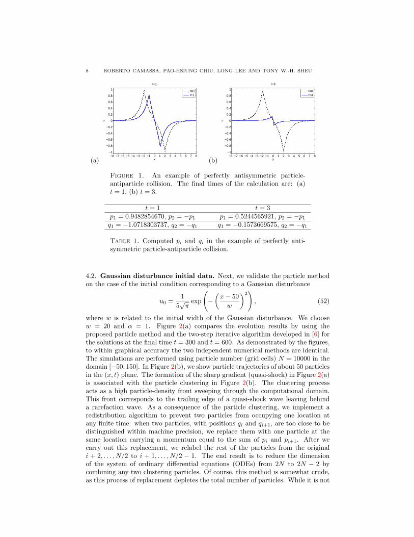
for which p1 = 1, p2 = −1, q1 = −2, and q2 = 2. This implies that the initial datafor p and q in the evolution equations (43) are p = 2 and q = −4. Substitutingthe initial p and q into equation (45) and (48), we obtain C ∼ 2.018571138566857and t0 ∼ 1.663801583149832. Therefore, when t = 1, we solve equations (45) and(48) to obtain q ∼ 2.1436607474 and p ∼ 1.89657093400691, which implies q1 ∼−1.0718303737, q2 ∼ 1.0718303737, p1 ∼ 0.9482854670, and p2 ∼ −0.9482854670.In Figure 1, we solve the evolution equation (37) with the initial momenta p1 = −1,p2 = 1, and particle positions q1 = −2, q2 = 2. The final times of the calculationare: (a) t = 1, (b) t = 3. Solutions of the PDE (39) u are found by equation(38) with 8001 grid points (xi, i = 1 · · · 8001) in the domain [−8, 8]. The timeintegrator is a fourth-order Runge-Kutta method. Our numerical solutions confirmthat pi and qi computed from the evolution equations (37) are identical to thosecomputed from the exact expressions (45) and (48), within fourteen decimal digits(machine precision). We summarize the calculation in Table 1.

8 ROBERTO CAMASSA, PAO-HSIUNG CHIU, LONG LEE AND TONY W.-H. SHEU

(a)−8 −7 −6 −5 −4 −3 −2 −1 0 1 2 3 4 5 6 7 8

−1

−0.8

−0.6

−0.4

−0.2

0

0.2

0.4

0.6

0.8

1

t=1

x

u

t=0t=1

(b)−8 −7 −6 −5 −4 −3 −2 −1 0 1 2 3 4 5 6 7 8

−1

−0.8

−0.6

−0.4

−0.2

0

0.2

0.4

0.6

0.8

1

t=3

x

u

t=0t=3

Figure 1. An example of perfectly antisymmetric particle-antiparticle collision. The final times of the calculation are: (a)t = 1, (b) t = 3.

t = 1 t = 3p1 = 0.9482854670, p2 = −p1 p1 = 0.5244565921, p2 = −p1q1 = −1.0718303737, q2 = −q1 q1 = −0.1573669575, q2 = −q1

Table 1. Computed pi and qi in the example of perfectly anti-symmetric particle-antiparticle collision.

4.2. Gaussian disturbance initial data. Next, we validate the particle methodon the case of the initial condition corresponding to a Gaussian disturbance

u0 =1

5√π

exp

(−(x− 50

w

)2), (52)

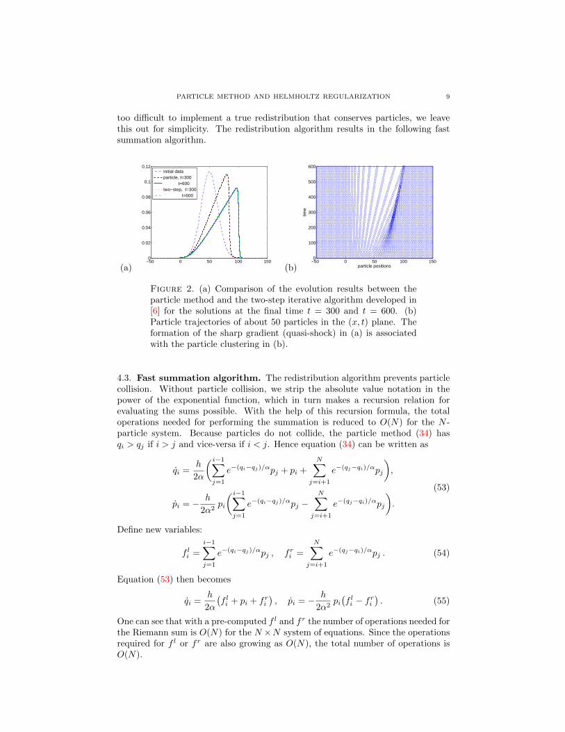
where w is related to the initial width of the Gaussian disturbance. We choosew = 20 and α = 1. Figure 2(a) compares the evolution results by using theproposed particle method and the two-step iterative algorithm developed in [6] forthe solutions at the final time t = 300 and t = 600. As demonstrated by the figures,to within graphical accuracy the two independent numerical methods are identical.The simulations are performed using particle number (grid cells) N = 10000 in thedomain [−50, 150]. In Figure 2(b), we show particle trajectories of about 50 particlesin the (x, t) plane. The formation of the sharp gradient (quasi-shock) in Figure 2(a)is associated with the particle clustering in Figure 2(b). The clustering processacts as a high particle-density front sweeping through the computational domain.This front corresponds to the trailing edge of a quasi-shock wave leaving behinda rarefaction wave. As a consequence of the particle clustering, we implement aredistribution algorithm to prevent two particles from occupying one location atany finite time: when two particles, with positions qi and qi+1, are too close to bedistinguished within machine precision, we replace them with one particle at thesame location carrying a momentum equal to the sum of pi and pi+1. After wecarry out this replacement, we relabel the rest of the particles from the originali + 2, . . . , N/2 to i + 1, . . . , N/2 − 1. The end result is to reduce the dimensionof the system of ordinary differential equations (ODEs) from 2N to 2N − 2 bycombining any two clustering particles. Of course, this method is somewhat crude,as this process of replacement depletes the total number of particles. While it is not

PARTICLE METHOD AND HELMHOLTZ REGULARIZATION 9

too difficult to implement a true redistribution that conserves particles, we leavethis out for simplicity. The redistribution algorithm results in the following fastsummation algorithm.

(a)−50 0 50 100 1500

0.02

0.04

0.06

0.08

0.1

0.12

initial dataparticle, t=300 t=600two−step, t=300 t=600

(b)−50 0 50 100 1500

100

200

300

400

500

600

particle positions

time

Figure 2. (a) Comparison of the evolution results between theparticle method and the two-step iterative algorithm developed in[6] for the solutions at the final time t = 300 and t = 600. (b)Particle trajectories of about 50 particles in the (x, t) plane. Theformation of the sharp gradient (quasi-shock) in (a) is associatedwith the particle clustering in (b).

4.3. Fast summation algorithm. The redistribution algorithm prevents particlecollision. Without particle collision, we strip the absolute value notation in thepower of the exponential function, which in turn makes a recursion relation forevaluating the sums possible. With the help of this recursion formula, the totaloperations needed for performing the summation is reduced to O(N) for the N -particle system. Because particles do not collide, the particle method (34) hasqi > qj if i > j and vice-versa if i < j. Hence equation (34) can be written as

qi =h

2α

(i−1∑j=1

e−(qi−qj)/αpj + pi +

N∑j=i+1

e−(qj−qi)/αpj

),

pi = − h

2α2pi

(i−1∑j=1

e−(qi−qj)/αpj −N∑

j=i+1

e−(qj−qi)/αpj

).

(53)

Define new variables:

f li =

i−1∑j=1

e−(qi−qj)/αpj , fri =

N∑j=i+1

e−(qj−qi)/αpj . (54)

Equation (53) then becomes

qi =h

2α

(f li + pi + fri

), pi = − h

2α2pi(f li − fri

). (55)

One can see that with a pre-computed f l and fr the number of operations needed forthe Riemann sum is O(N) for the N ×N system of equations. Since the operationsrequired for f l or fr are also growing as O(N), the total number of operations isO(N).

10 ROBERTO CAMASSA, PAO-HSIUNG CHIU, LONG LEE AND TONY W.-H. SHEU

We now establish the recursion relation for f l and fr:

f li+1 =

i∑j=1

e−(qi+1−qi)/αpj

=

i−1∑j=1

e−(qi+1−qj)/αpj + e−(qi+1−qi)/αpi

=

i−1∑j=1

e−(qi+1−qi)/α−(qi−qj)/αpj + e−(qi+1−qi)/αpi

= e−(qi+1−qi)/α(i−1∑j=1

e−(qi−qj)/αpj + pi

)= e−(qi+1−qi)/α

(f li + pi

).

(56)

Similarly,fri+1 = e−(qi−qi+1)/αfri − pi+1. (57)

Because e−(qi−qi+1)/α leads to an exponential growth, for numerical stability therecursion relation for fr is better solved backward as

fri =(fri+1 + pi+1

)e−(qi+1−qi)/α. (58)

4.4. Dynamics of momentum-like variable. In the paper [6], we demonstratethat for smooth nearly square-wave initial data,

u0(x) =1

2

(tanh

(x+ 15

w

)− tanh

(x− 15

w

)), (59)

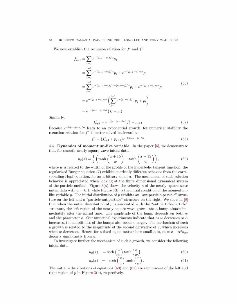
where w is related to the width of the profile of the hyperbolic tangent function, theregularized Burger equation (7) exhibits markedly different behavior from the corre-sponding Hopf equation, for an arbitrary small α. The mechanism of such solutionbehavior is appreciated when looking at the finite dimensional dynamical systemof the particle method. Figure 3(a) shows the velocity u of the nearly square-waveinitial data with w = 0.1, while Figure 3(b) is the initial condition of the momentum-like variable p. The initial distribution of p exhibits an “antiparticle-particle” struc-ture on the left and a “particle-antiparticle” structure on the right. We show in [6]that when the initial distribution of p is associated with the “antiparticle-particle”structure, the left region of the nearly square wave grows into a hump almost im-mediately after the initial time. The amplitude of the hump depends on both wand the parameter α. Our numerical experiments indicate that as w decreases or αincreases, the amplitudes of the humps also become larger. The mechanism of sucha growth is related to the magnitude of the second derivative of u, which increaseswhen w decreases. Hence, for a fixed α, no matter how small α is, m = u− α2uxxdeparts significantly from u.

To investigate further the mechanism of such a growth, we consider the followinginitial data

u0(x) = sech( xw

)tanh

( xw

), (60)

u0(x) = −sech( xw

)tanh

( xw

). (61)

The initial p distributions of equations (60) and (61) are reminiscent of the left andright region of p in Figure 3(b), respectively.

PARTICLE METHOD AND HELMHOLTZ REGULARIZATION 11

(a)−30 −20 −10 0 10 20 300

0.5

1

1.5

x

u

(b)−30 −20 −10 0 10 20 30

−40

−30

−20

−10

0

10

20

30

40

x

p

Figure 3. (a) The velocity u of the nearly square-wave initialdata with w = 0.1. (b) The initial condition of the momentum-likevariable p. The initial distribution of p exhibits a “antiparticle-particle” structure on the left and a “particle-antiparticle” struc-ture on the right.

(a)−40 −20 0 20 40−1

−0.5

0

0.5

1sech(x)tanh(x)

x

u

t=0t=5t=10

(b)−40 −20 0 20 40

−25

−20

−15

−10

−5

0

5

10

15

20

25sech(x)tanh(x)

x

p

t=0t=5t=10

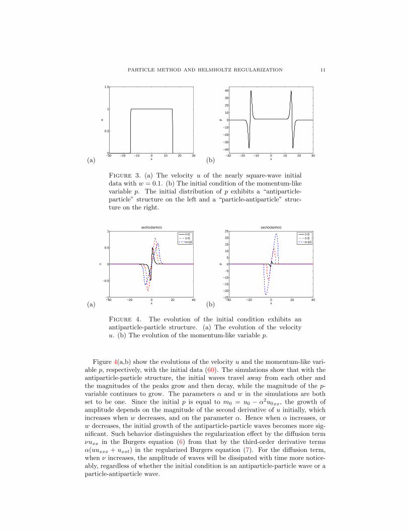
Figure 4. The evolution of the initial condition exhibits anantiparticle-particle structure. (a) The evolution of the velocityu. (b) The evolution of the momentum-like variable p.

Figure 4(a,b) show the evolutions of the velocity u and the momentum-like vari-able p, respectively, with the initial data (60). The simulations show that with theantiparticle-particle structure, the initial waves travel away from each other andthe magnitudes of the peaks grow and then decay, while the magnitude of the p-variable continues to grow. The parameters α and w in the simulations are bothset to be one. Since the initial p is equal to m0 = u0 − α2u0xx, the growth ofamplitude depends on the magnitude of the second derivative of u initially, whichincreases when w decreases, and on the parameter α. Hence when α increases, orw decreases, the initial growth of the antiparticle-particle waves becomes more sig-nificant. Such behavior distinguishes the regularization effect by the diffusion termνuxx in the Burgers equation (6) from that by the third-order derivative termsα(uuxxx + uxxt) in the regularized Burgers equation (7). For the diffusion term,when ν increases, the amplitude of waves will be dissipated with time more notice-ably, regardless of whether the initial condition is an antiparticle-particle wave or aparticle-antiparticle wave.

12 ROBERTO CAMASSA, PAO-HSIUNG CHIU, LONG LEE AND TONY W.-H. SHEU

(a)−40 −20 0 20 40−1

−0.5

0

0.5

1−sech(x)tanh(x)

x

u

t=0t=5t=10

(b)−40 −20 0 20 40

−2.5

−2

−1.5

−1

−0.5

0

0.5

1

1.5

2

2.5−sech(x)tanh(x)

x

p

t=0t=5t=10

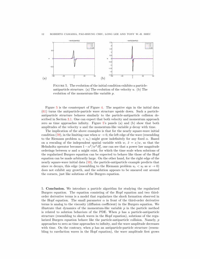
Figure 5. The evolution of the initial condition exhibits a particle-antiparticle structure. (a) The evolution of the velocity u. (b) Theevolution of the momentum-like variable p.

Figure 5 is the counterpart of Figure 4. The negative sign in the initial data(61) turns the anitparticle-particle wave structure upside down. Such a particle-antiparticle structure behaves similarly to the particle-antiparticle collision de-scribed in Section 3.1. One can expect that both velocity and momentum approachzero as time approaches infinity. Figure 5’s panels (a) and (b) show that bothamplitudes of the velocity u and the momentum-like variable p decay with time.

The implication of the above examples is that for the nearly square-wave initialcondition (59), in the limiting case when w → 0, the left edge of the wave (resemblingto the Riemann problem ul < ur) might grow indefinitely for any fixed α. Basedon a rescaling of the independent spatial variable with w, x = x/w, so that theHelmholtz operator becomes 1−α2/w2 ∂2x, one can see that a power law magnitudeorderings between w and α might exist, for which the time scale when solutions ofthe regularized Burgers equation can be expected to behave like those of the Hopfequation can be made arbitrarily large. On the other hand, for the right edge of thenearly square-wave initial data (59), the particle-antiparticle example predicts thatsince m decays, this edge (resembling to the Riemann problem ur < ul as w → 0)does not exhibit any growth, and the solution appears to be smeared out aroundthe corners, just like solutions of the Burgers equation.

5. Conclusion. We introduce a particle algorithm for studying the regularizedBurgers equation. The equation consisting of the Hopf equation and two third-order derivative terms is a model that regularizes the shock formation observed inthe Hopf equation. The small parameter α in front of the third-order derivativeterms is analog to the viscosity (diffusion coefficient) in the Burgers equation. Weillustrate that dynamics of the momentum-like variable p in the particle methodis related to solution behaviors of the PDE. When p has a particle-antiparticlestructure (resembling to shock waves in the Hopf equation), solutions of the regu-larized Burgers equation behave like the particle-antiparticle collision. Namely, papproaches to zero as time approaches to infinity, and the wave amplitude decreaseswith time. On the contrary, when p has an antiparticle-particle structure (resem-bling to rarefaction waves in the Hopf equation), the wave amplitude first grows

PARTICLE METHOD AND HELMHOLTZ REGULARIZATION 13

and then decays 1. Such behavior is different from that of the Burgers equation,where viscosity dissipates both shock waves and rarefaction waves immediately.

Acknowledgements. This research is partially supported by NSF through GrantDMS-0610149 (LL) and DMS-0509423 (RC). T.W.H. Sheu would like to thankthe Department of Mathematics at the University of Wyoming for its provision ofexcellent research facilities during his visiting professorship.

REFERENCES

[1] H. S. Bhat and R. C. Fetecau, A Hamiltonian regularization of the Burgers equation, J.

Nonlinear Sci., 16 (2006), 615–638.[2] H. S. Bhat and R. C. Fetecau, The Riemann problem for the Leray-Burgers equation, J.

Differential Equations, 246 (2009), 3957–3979.

[3] R. Camassa, Characteristics and initial value problem of a completely integrable shallow waterequation, Discrete Contin. Dyn. Syst. Ser. B, 3 (2003), 115–139.

[4] R. Camassa, J. Huang and L. Lee, On a completely integral numerical scheme for a nonlinear

shallow-water wave equation, J. Nonlin. Math. Phys., 12 (2005), 146–162.[5] R. Camassa, J. Huang and L. Lee, Integral and integrable algorithm for a nonlinear shallow-

water wave equation, J. Comp. Phys., 216 (2006), 547–572.

[6] R. Camassa, P. H. Chiu, L. Lee and T. W. H. Sheu, Viscous and inviscid regularizations in aclass of evolutionary partial differential equations, J. Comp. Phys., 229 (2010), 6676–6687.

[7] A. Degasperis, D. D. Holm and A. N. W. Hone, Integrable and non-integrable equations withpeakons, in “Nonlinear Physics: Theory and Experiment, II” (Gallipoli, 2002), World Sci

Publishing, River Edge, NJ, (2003), 37–43.

[8] H. Holden and X. Raynaud, A convergent numerical scheme for the Camassa-Holm equationbased on multipeakons, Discrete Contin. Dyn. Syst., 14 (2006), 505–528.

[9] H. Holden and X. Raynaud, Convergence of a finite difference scheme for the Camassa-Holm

equation, SIAM J. Numer. Anal., 44 (2006), 1655–1680.[10] J. Leray, Essai sur le mouvement d’un fluid visqueux emplissant l’space, Acat Math., 63

(1934), 93–258.

[11] K. Mohseni, H. Zhao and J. Marsden, Shock regularization for the Burgers equation, AIAAPaper 2006–1516, 44th AIAA Aerospace Science Meeting and Exibit Reno, Nevada, Jan, 9–12,

2006.

[12] G. Norgard and K. Mohseni, A regularization of the Burgers equation using a filtered con-vective velocity, J. Phys. A: Math. Theor., 41 (2008), 344016, 21pp.

Received xxxx 20xx; revised xxxx 20xx.

E-mail address: camassa@amath.unc.edu

E-mail address: phchiu@iner.gov.tw

E-mail address: llee@uwyo.edu

E-mail address: twhsheu@ntu.edu.tw

1 In the course of assembling references for submission of this work, we became aware of therecent paper [2] where similar observations were made and investigated.