A Practical Iterative Algorithm for the Art Gallery ... · A Practical Iterative Algorithm for the...

Noname manuscript No.(will be inserted by the editor)

A Practical Iterative Algorithm for the Art Gallery Problem usingInteger Linear Programming

Davi C. Tozoni · Pedro J. de Rezende · Cid C. deSouza

January 14, 2014

Abstract In the last few decades, the search for exact algorithms for known NP-hard geometric problemshas intensified. Many of these solutions make use of Integer Linear Programming (ILP) modeling and relyon state of the art solvers to be able to find optimal solutions for large instances in a matter of minutes.In this work, an ILP based algorithm is proposed to optimally solve the Art Gallery Problem (AGP), oneof the most studied problems in Computational Geometry. The basic idea of our method is to iterativelygenerate upper and lower bounds for the problem through the resolution of discretized versions of theAGP, which are reduced to instances of the Set Cover Problem. Our algorithm was implemented andtested on almost three thousand instances and attained optimal solutions for the vast majority of them,greatly increasing the set of instances for which exact solutions are known. To the best of our knowledge,in spite of the extensive study of the AGP in the last four decades, no other algorithm has shown theability to solve the AGP as effectively and efficiently as the one described here. Evidence of its robustnessis presented through tests done on a number of classes of polygons of various sizes with and withoutholes.

Keywords Art Gallery Problem, Exact Algorithm, Combinatorial Optimization, ComputationalGeometry

This research was supported by grants from Conselho Nacional de Desenvolvimento Científico e Tecnológico (CNPq)#477692/2012-5, #302804/2010-2, Fundação de Amparo à Pesquisa do Estado de São Paulo (Fapesp) #2007/52015-0,#2012/18384-7, and Faepex/Unicamp.

Institute of Computing, University of CampinasCampinas, [email protected], {rezende | cid}@ic.unicamp.br

2 Tozoni, D. C., de Rezende, P. J., de Souza, C. C.

1 Introduction

In 1973, Victor Klee proposed a new geometric puzzle, which basically consisted in answering how fewguards would be sufficient to ensure that an art gallery (represented by a simple polygon) be fully guarded,assuming that a guard’s field of view covers 360 degrees as well as an unbounded distance. This questionbecame known as the Art Gallery Problem (AGP) and, in the course of time, it turned into one of themost investigated problems in computational geometry. The breadth of this research can be perceivedfrom the many important works that appeared, including O’Rourke’s classical book [16], a recent text byGhosh on visibility algorithms [10] and surveys by Shermer in 1992 [17] and Urrutia in 2000 [19].

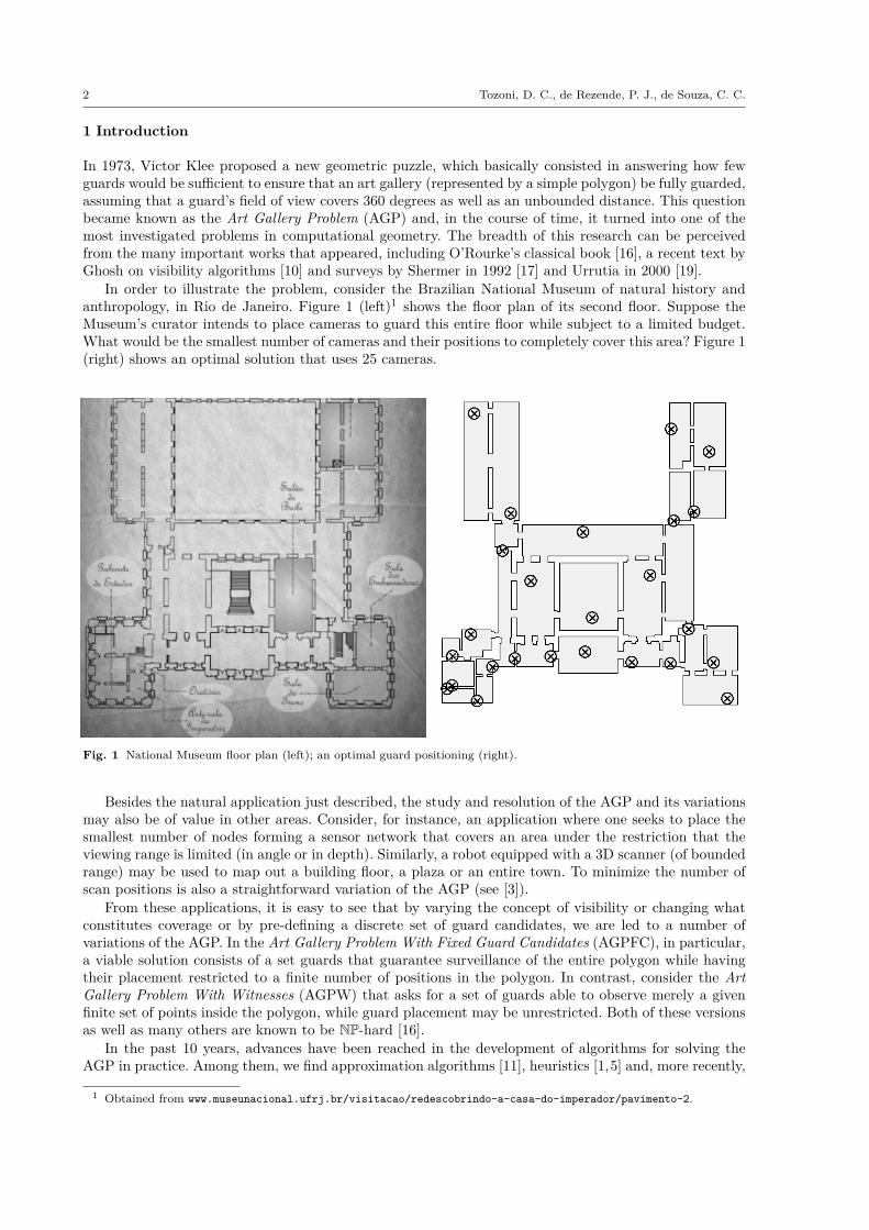
In order to illustrate the problem, consider the Brazilian National Museum of natural history andanthropology, in Rio de Janeiro. Figure 1 (left)1 shows the floor plan of its second floor. Suppose theMuseum’s curator intends to place cameras to guard this entire floor while subject to a limited budget.What would be the smallest number of cameras and their positions to completely cover this area? Figure 1(right) shows an optimal solution that uses 25 cameras.

Fig. 1 National Museum floor plan (left); an optimal guard positioning (right).

Besides the natural application just described, the study and resolution of the AGP and its variationsmay also be of value in other areas. Consider, for instance, an application where one seeks to place thesmallest number of nodes forming a sensor network that covers an area under the restriction that theviewing range is limited (in angle or in depth). Similarly, a robot equipped with a 3D scanner (of boundedrange) may be used to map out a building floor, a plaza or an entire town. To minimize the number ofscan positions is also a straightforward variation of the AGP (see [3]).

From these applications, it is easy to see that by varying the concept of visibility or changing whatconstitutes coverage or by pre-defining a discrete set of guard candidates, we are led to a number ofvariations of the AGP. In the Art Gallery Problem With Fixed Guard Candidates (AGPFC), in particular,a viable solution consists of a set guards that guarantee surveillance of the entire polygon while havingtheir placement restricted to a finite number of positions in the polygon. In contrast, consider the ArtGallery Problem With Witnesses (AGPW) that asks for a set of guards able to observe merely a givenfinite set of points inside the polygon, while guard placement may be unrestricted. Both of these versionsas well as many others are known to be NP-hard [16].

In the past 10 years, advances have been reached in the development of algorithms for solving theAGP in practice. Among them, we find approximation algorithms [11], heuristics [1,5] and, more recently,

1 Obtained from www.museunacional.ufrj.br/visitacao/redescobrindo-a-casa-do-imperador/pavimento-2.

A Practical Iterative Algorithm for the Art Gallery Problem 3

some advances in the search for exact algorithms [8,13]. However, none of the algorithms proposed tosolve the original AGP, where guards are free to be placed anywhere inside the polygon, was able toconsistently find optimal solutions for large instances within a reasonable amount of time.

In this paper, we describe a new practical algorithm for solving the original AGP to exactness. Itfollows an iterative process of obtaining lower and upper bounds that lead to an optimal solution. Thesebounds are drawn up through the resolution of instances of the aforementioned AGPW and AGPFCproblems using Integer Linear Programming (ILP) techniques. As we shall see in Section 5, optimalsolutions are reached (in a reasonable amount of time) for almost the totality of the publicly availableinstances. These results consist in a significant improvement over the previously published techniques.Not only the proposed algorithm solved instances with up to 2500 vertices, something without precedentin the literature, but it also proved to be quite robust, achieving optimality in more than 98% of the2400+ instances tested.

In the next section, we briefly survey relevant related works. Section 2 is dedicated to presenting afew basic concepts and notations while Section 4 describes the main steps of the proposed algorithm.A discussion of the computational results obtained in our experiments appear in Section 5. Lastly, inSection 6, we draw some conclusions and identify future directions of research.

2 Related Work

As early as 1975, Chvátal proved that bn/3c guards are always sufficient and sometimes necessary forcovering a simple polygon of n vertices. Roughly a decade later, Lee and Lin proved the NP-hardness ofthe AGP for vertex guards [14]. The case of point guards and of edge guards are also known to be equallyhard [16].

After progress on theoretical results regarding the complexity of the AGP, researchers turned theirattention to the development of algorithms for positioning guards and trying to reach solutions as closeas possible to optimality. Ghosh, in 1987, proposed a logn-approximation algorithm for the AGP withvertex or edge guards [9]. The idea, also exploited in more recent for exact algorithms, was to reduce theAGP to the Set Cover Problem (SCP) and to apply an already known approximation for the SCP.

In 2007, Amit et al. [1] proposed a set of heuristics based on greedy strategies and polygon partitionmethods. Four years later, Bottino and Laurentini [5] proposed a new heuristic for the restricted versionof the AGP where the objective is to cover only the edges of the polygon. Both algorithms were a stepforward and the latter, in particular, was able to find optimal solutions for a considerable number ofinstances.

Recently, however, the search for algorithms that are able to find provably optimal solutions forspecific formulations has intensified. In this line, two results are worth highlighting. In 2011, Couto etal. [8], published the first exact algorithm for the Art Gallery Problem with Vertex-Guards (AGPVG)with verified practical efficiency. They devised an iterative technique that was guaranteed to convergeto an optimal solution. While the maximum number of iterations was proven to be polynomial in thenumber of vertices in the worst case, actual convergence happened after just a few iterations. The firstinteresting insight was to show that the infinite points of the polygon to be watched could be discretizedinto a finite set of points, called witnesses. The AGPVG, having a finite number of possible guards,coupled with the now finite number of witnesses to be covered, was reduced (in the Karp sense) toa sequence of SCP instances that could be solved to optimality using an Integer Programming solver.These instances started off with a small subset of witnesses and simply included additional witnesseswhenever the previous solution was not viable for the original instance. An alternative approach consistedof including all pre-determined witness into a single SCP instance and solving the problem to exactnessin a single shot. In fact, in [8], a clever reduction of the witness set is also presented, which makes thisalternative approach much more competitive timewise. These algorithms for the AGPVG were tested onmore than ten thousand polygons of various classes and, for up to 2500 vertices, optimal solutions wereattained in just a few minutes of computer time.

Through a related approach, Kröller et al. [13] tackled the original art gallery problem by seeking toreduce the infinite number of witnesses and guard candidates into finite sets, thus generating instancesof the discretized AGP, which can be reduced to SCP instances as mentioned above. By solving thelinear relaxation of the primal and dual formulations of the SCP instances created, their method is ableto find upper and lower bounds for the original problem. The method is also iterative and adds new


witnesses and guards at each new iteration, in hope that the an integer solution for the relaxed AGPis found. A negative result is inferred after a pre-established execution time limit is exceeded. Althoughtheir algorithm converged in several instances, giving rise to an increase in the number of instances forwhich optimal solutions are known, unfortunately, for many polygons the method was unable to convergeto integer solutions.

This brief summary of the state of the art on exact solutions for the original AGP sets the stage forthe contributions that this paper brings forth.

3 Terminology and Formulation

Recall that the objective of the Art Gallery Problem is to find the minimum number of guards that aresufficient to ensure visual coverage of a given gallery, represented as a simple polygon P (possibly withholes). Consider that the vertex set V of P has cardinality n.

Two points in P are visible to each other if the line segment that joins them does not intersect theexterior of P . The visibility polygon of a point p ∈ P , denoted by Vis(p), is the set of all points in P thatare visible from p. The edges of Vis(p) are called visibility edges and are said to be proper for p if theyare not contained in any edges of P .

Given a finite set S of points in P , a covered (respectively, uncovered) region induced by S in P is amaximal connected region in ∪

p∈SVis(p) (respectively, P − ∪

p∈SVis(p)).

Fig. 2 A polygon with holes (left); the visibility polygon of a point (center); and the arrangement induced by a finite setS of points (right).

Moreover, the geometric arrangement defined by the visibility edges of the points in S, denoted Arr(S),partitions P into a collection of closed polygonal faces called Atomic Visibility Polygons or simply AVPs.Denote by Cf ⊂ S the set of points in S that cover an AVP f . Define a partial order ≺ on the facesof Arr(S) as follows. Given two AVPs f and f ′, we say that f ≺ f ′ if and only if Cf ′ ⊂ Cf . We call fa shadow face (light face) if f is minimal (maximal) with respect to ≺. Figures 2 and 3 illustrate theseconcepts.

One important observation for the complexity analysis of our algorithm is that, for a given set S ⊆ P ,the time needed to built Arr(S), as well as the number of AVPs in this arrangement, is O((|S| + |P |)3)[4].

3.1 ILP Formulation

In a geometric setting, the AGP can be restated as the problem of determining a smallest set of pointsG ⊂ P such that ∪

g∈GVis(g) equals P . This leads to a reduction from the AGP to the SCP, in which the

points in P are the elements to be covered and the visibility polygons of the points in P are the sets used


Fig. 3 A set S of three points and its covered (gray) and uncovered (white) regions (left); and the arrangement inducedby S with the light (gray) and shadow (dark gray) AVPs (right).

for covering. Accordingly, we can use this reduction to construct an ILP formulation for the AGP:

min∑c∈P

xc

s.t.∑c∈P

w∈Vis(c)

xc ≥ 1, ∀w ∈ P

xc ∈ {0, 1}, ∀c ∈ P

However, this formulation has an infinite number of constraints and an infinite number of variables,rendering it of no practical benefit. A natural idea that arises is to make at least one of these quantitiesfinite. By fixing only the guard candidates to be a finite set, we obtain the so-called Art Gallery ProblemWith Fixed Guard Candidates (AGPFC). On the other hand, by restricting solely the witness set to afinite set, we end up with the special AGP variant known as the Art Gallery Problem With Witnesses(AGPW). In principle, in the first case, we are still left with an infinite number of constraints while,in the second case, we still have an infinite number of variables. However, in order to have a tractableSCP instance, one should have both the witness and the guard candidate sets of finite size. The AGPvariant that fulfills this property is named the Art Gallery Problem with Witnesses and Fixed GuardCandidates (AGPWFC). Examples of these three versions of the AGP are shown in Figure 4. Therein,the witnesses and the guard candidates are identified by the symbols “×” and “⊗”, respectively. Darkerguard candidates refer to guards present in an optimal solution of the corresponding problem and, whenappropriate, have their visibility polygons also depicted.

A remarkable theoretical result discussed in the next section is that any instance of the AGPW orof the AGPFC can be reduced in polynomial time to an instance of the AGPWFC. This means that, tosolve the AGPW or the AGPFC, one actually has to find an optimal solution of a polynomial-sized SCPinstance. Now, notice that the optimum of an AGPW instance always yields a lower bound for the originalAGP value, since it is clearly a relaxation of the latter. On the other hand, if the set of guard candidatescovers the polygon P , an optimal value for the AGPFC is feasible for the original AGP instance and,therefore, provides an upper bound for it. These are relevant observations since modern ILP solvers arecapable to handle very large-sized SCP instances such as AGPWFC instances, for that matter. As wewill see later, our algorithm relies on these facts.

To close this section, a couple of additional notations are introduced. Let D and C be finite witnessand guard candidate sets, respectively. We denote the AGPW, AGPFC and AGPWFC problems definedfor the sets C and D by AGPW(D), AGPFC(C) and AGPWFC(D,C), respectively. The SCP modelassociated to AGPWFC(D,C) is then

min∑c∈C

xc,

s.t.∑c∈C

w∈Vis(c)

xc ≥ 1, ∀w ∈ D,

xc ∈ {0, 1}, ∀c ∈ C.


Fig. 4 An illustration of the four different variants of the Art Gallery Problem: (a) AGP; (b) AGPFC; (c) AGPW; (d)AGPWFC.

4 A Practical Iterative Algorithm for AGP

The purpose of this section is to describe our algorithm, which basically consists of iteratively obtainingincreasing lower (dual) and decreasing upper (primal) bounds for the AGP. These steps are repeated untileither the gap between the bounds reaches zero or the time limit is exceeded. New bounds are obtainedby solving discretized versions of the original AGP. To find a new lower bound, an AGPW instance issolved, while in the upper bound case, an AGPFC instance is worked out in which the guard candidateset covers the polygon. One important fact to remember is that an optimal solution for such an instanceof AGPFC is also viable for AGP, since the AGPFC asks for a solution that guards the entire polygon.Consequently, reducing the gap to zero means reaching an optimal solution for the original AGP.

In Algorithm 1, we present a simplification of how our technique works. After initializing the witnessand guard candidate sets, the algorithm enters its main loop (lines 4 to 10). At each iteration new lowerand upper bounds are computed and, if optimality has not been proved, the witness and guard candidatesets are updated in line 8. Later we will see how this can be done in a way that the duality gap decreasesmonotonically through the iterations. It is also worth noticing that, as we still do not have a proof ofconvergence for the algorithm, the parameter MAXTIME is used to limit its running time.

ALGORITHM 1: AGP Algorithm1: Set UB← |V | and LB← 02: Select the initial witness set D3: Select the initial guard candidate set C ⊇ V4: while (UB 6= LB) and (MAXTIME not reached) do5: Solve AGPW(D), set Gw ← optimal solution of AGPW(D) and LB← max{LB, |Gw|}6: Solve AGPFC(C), set Gf ← optimal solution of AGPFC(C and UB← min{UB, |Gf |}7: if (UB 6= LB) then8: Update D and C9: end if10: end while11: return Gf

In the following two subsections, the procedures for solving AGPW (line 5) and AGPFC (6) instancesare described in detail. Subsequently, Section 4.3 describes the resolution method for AGPWFC instancesthrough ILP techniques. As said in the previous section, both the AGPW and the AGPFC can be castas an AGPWFC, justifying why we focus on the latter. In Section 4.4, we present how the management


of witness set and, as a consequence, of the guard candidate set, is done. Lastly, Section 4.5 gathers allthe algorithmic information presented previously and describes the complete algorithm for the AGP.

4.1 Solving AGPW

Consider AGPW(D) the Art Gallery Problem instance where the objective is to cover all points in afinite set D. As said before, the resolution of an AGPW on D allows for the discovery of a new lowerbound for the AGP since fully covering P requires at least as many guards as the minimum sufficient tocover the points in D.

However, despite being a simplification of the original AGP problem, we are still dealing with aninfinite number of potential guard positions, which does not allow for a direct reduction to the set coverproblem. Thus, our approach is based on discretizing the guard candidate set, creating an AGPWFCinstance from our original AGPW. To do this, we apply Theorem 1.

Theorem 1 Let D be a finite subset of points in P . Then, there exists an optimal solution for AGPW(D)in which every guard belongs to a light AVP of Arr(D).

Proof Let G be an optimal (cardinality-wise) set of guards that covers all points in D. Suppose there isa guard g in G whose containing face F in Arr(D) is not a light AVP. This means that F is not maximalwith respect to ≺ (see Section 3). In other words, there exists a face F ′ of Arr(D) that shares an edgewith F such that F ≺ F ′, i.e., F ′ sees more points of D than F does. An inductive argument suffices toshow that this process eventually reaches a light AVP (maximal w.r.t. ≺) wherein lies a point that seesat least as much of D as g does, i.e., g may be replaced by a guard that lies on a light AVP. The Theoremthen follows, by induction, on the number of guards of G. ut

From Theorem 1, one concludes that there exists an optimal solution for AGPW(D) in which all theguards are in Light AVPs of the arrangement induced by D. Besides, as every point (whether inside oron the boundary) of an AVP can see the same set of witnesses, we can state that there is an optimalsolution G where each point in G belongs to the set VL(D) of all vertices from the light AVPs of Arr(D).Therefore, an optimal solution for AGPW(D) can be obtained simply by solving AGPWFC(D,VL(D)).As seen before, the latter problem can be modeled as an ILP, where the numbers of constraints and ofvariables are polynomial in |D|. This follows, as mentioned in Section 3, from the fact that the numberof AVPs (and vertices) in Arr(D) is bounded by a polynomial in |D| and |P |. Algorithm 2 shows apseudo-code of the AGPW resolution method.

ALGORITHM 2: AGPW(D) Algorithm1: Arr(D)← construct the arrangement from the visibility polygons of the points in D2: VL(D)← identify the vertices of the light AVPs of Arr(D)3: C ← VL(D)4: Solve AGPWFC(D, C): set Gw ← optimal solution of AGPWFC(D, C)5: return Gw

4.2 Solving AGPFC

As we now know how to generate dual bounds for the AGP, the next task is to compute good upperbounds for the problem. A possible way to achieve this is through the resolution of an AGPFC instancein which the guard candidate set is known to cover the polygon. As said earlier, under this condition, anAGPFC solution is always viable for the original problem.

In this context, consider AGPFC(C) the instance of AGPFC where the finite guard candidate set is C.In contrast to what was discussed regarding the AGPW, we now have a finite number of guard candidatesand an infinite number of points to be covered. Therefore, a straightforward resolution method using areduction to an SCP is not possible. To circumvent this, our algorithm discretizes the original AGPFCinstance, relying on what Theorem 2 establishes.


Theorem 2 Let D and C be two finite subsets of P , so that C fully covers P . Assume that G(D,C) isan optimal solution for AGPWFC(D,C). If G(D,C) also covers P , then G(D,C) is an optimal solutionfor AGPFC(C).

Proof Assume that G(D,C) covers P , but it is not an optimal solution for AGPFC(C). Then, thereexists G′ ⊆ C with |G′| < |G(D,C)| such that G′ is a feasible solution for AGPFC(C), i.e., G′ covers P .This implies that G′ is also a feasible solution for AGPWFC(D,C), contradicting the fact that G(D,C)is optimal for this problem. ut

Theorem 2 shows that an optimal solution for AGPFC may be obtained through the resolution of anAGPWFC instance, provided it fully covers P . Whenever an optimal solution for the simplified version(AGPWFC) leaves uncovered regions in P , additional work is required. To guarantee that we attain anoptimal solution for AGPFC, we will employ here a technique designed by Couto et al. [8] to solve theAGPVG, a special case of AGPFC where C = V , but which may be used to solve the general case withoutsignificant changes.

Initially, consider that we have a finite witness set D. Using the guard candidate set C, we cancreate and solve the AGPWFC(D,C) instance. If the solution fully covers polygon, we have satisfied thehypothesis of Theorem 2 and, consequently, we have an optimal solution for AGPFC. Otherwise, thereare regions of the polygon that remain uncovered. We now update the witness set, adding new pointswithin the uncovered regions, denoted CU (C), and repeat the process.

As shown in [8], the iterative method for solving AGPFC converges in polynomial time. To clarifythis point, consider the arrangement induced by all visibility polygons of guard candidates in C. Thisarrangement partitions the polygon into O((|C| · n)2) faces (AVPs). These faces have the property thatif any of its point is covered, the entire face is covered. Therefore, our aim is to iteratively construct Dby choosing witnesses in the interior of AVPs of Arr(C), leading to an AGPWFC instance whose optimalsolution will also be viable and optimal for the AGPFC. While the number of iterations is clearly inO((|C| · n)2), in [8] it is shown that, in practice, this number is much lower. Moreover, it can even beargued that it suffices to select one point from each shadow AVP of the arrangement induced by C. See[8], for details.

A pseudo-code for the algorithm used to solve the AGPFC is shown in Algorithm 3.

ALGORITHM 3: AGPFC(C) Algorithm1: Df ← initial witness set2: repeat3: Solve AGPWFC(Df , C): set Gf ← optimal solution4: if Gf does not fully cover P then5: Df ← Df ∪ CU (Gf )6: end if7: until Gf fully covers P8: return Gf

4.3 Solving AGPWFC (SCP)

Having reduced both AGPW and AGPFC problems into AGPWFC instances in order to obtain thedesired bounds, the objective becomes solving the latter efficiently. Since an AGPWFC(D,C) instancecan easily be reduced to an SCP, where the witnesses in D are the elements to be covered and thevisibility polygons of the guard candidates in C are the subsets considered, we will make use of the ILPformulation for SCP presented in Section 3.

A simple and straightforward approach would be to directly use an ILP solver, such as XPRESS orCPLEX, since even large instances of the (NP-hard) SCP can be solved quite efficiently by many moderninteger programming solvers. However, as observed in our experiments, some AGP instances can generatesignificantly complex and very large SCP instances, rendering the solvers less efficient. For this reason,some known techniques were implemented to improve the solvers’ running time. Among these, the mosteffective consisted in the reduction on the number of constraints and variables in the initial model. A


simple primal heuristic based on Lagrangian relaxation was also implemented to obtain viable solutions.Despite the fact that these are standard techniques to ILP practitioners, some of them proved to beinstrumental in the context of the AGP. So, for completeness, we briefly describe them below.

The method used for reducing constraints and variables is based on containment relationships betweencolumns (guard candidates) and between rows (witnesses) of the Boolean constraint matrix correspondingto the ILP model of the SCP instance.

Firstly, we search for and discard redundant guard candidates (columns). A guard candidate gr isredundant if there is another candidate that covers the same witness set as gr. For this step, we divideall guard candidates into groups, according to the light AVP they belong to. Guard candidates fromthe same AVP are then tested pairwise for redundancy, and, when one is found, it is removed from theoriginal matrix. Here a slight improvement applies to SCP instances arising from the AGPW. Rememberthat when lower bounds are computed, the witness set D remains fixed while the guard candidates arethe vertices of the light AVPs in Arr(D). In this case, by definition, all vertices of a given light AVPcover the same subset of witnesses. Hence, all but one of the corresponding variables is redundant inthe SCP instance, i.e., we are left with a single vertex from each light AVP. This reduces the size of theguard candidate set by a factor of at least three, although the remaining subset still needs to be checkedpairwise for redundancy.

After the removal of columns, we also test each pair of rows in search for removable ones. We say thata row represents an easy witness w whenever the set of guard candidates that see w properly containsthe (whole) set of candidates that see some other witness.

It is important to notice that the test for redundant candidates (columns) and easy witnesses (rows)can be performed simply by using very fast bit string operations.

Besides conducting matrix reduction, our algorithm also uses an initial Lagrangian Heuristic (LH)with the goal of finding good (or optimal) viable solutions for the AGPWFC. The heuristic implementedis based on the work by Beasley [2], which, among other results, presents a Lagrangian Relaxation forSCP. The idea of the relaxation is to move all coverage constraints into the objective function and usepenalties uw (for each constraint), the Lagrangian Multipliers (LM), resulting in the following LagrangianPrimal Problem (LPP):

z(u) = min∑c∈C

xc +∑w∈D

uw

(1−

∑c∈C

w∈Vis(c)

xc

)

xc ∈ {0, 1},∀c ∈ C

After this step, the LPP (with no actual constraints) can be solved by inspection. It is well-knownthat the optimum of this problem gives a lower bound for the original SCP instance. The new quest isto find the values for LM (uw variables) that maximize this lower bound. The optimization problem offinding the best Lagrangian Multipliers is called Lagrangian Dual Problem (LDP):

Z = max z(u)uw ≥ 0, ∀w ∈W.

A classical approach to tackle the LDP is to apply the subgradient method (c.f., [2]), which is analgorithm in which the LM values are updated iteratively using a subgradient of the objective function.In this way, at each iteration, a new LPP instance is solved and, based on this result, we apply a primalheuristic, which attempts to find a new viable solution for the original SCP instance. The primal heuristicconsists in a greedy algorithm that uses the Lagrangian costs obtained during the last LPP resolutionto define which candidates will be selected to join the new viable solution (see [2] for more details). Insummary, at each iteration, a new lower bound for the SCP is obtained from the LPP resolution anda new upper bound is obtained by the primal heuristic. The subgradient method stops when either anoptimal solution is found or a maximum number of iterations has been reached.

After running the subgradient method for solving LDP, we have a reduced ILP matrix and an up-per bound for AGPWFC. This information can be used in the ILP Solver to improve its performance.Algorithm 4 summarizes the steps for solving the AGPWFC instance, using matrix reduction and aLagrangian Heuristic.


ALGORITHM 4: AGPWFC(D,C) Algorithm1: M ← Boolean matrix of the SCP model constructed using D and C2: R← matrix obtained from M after applying the reduction procedure3: Set I ← SCP instance associated to R4: Solve I using LH5: Set LBSCP ← best lower bound found for I by the subgradient method6: Set Gv ← best viable solution found for I by the primal heuristic7: Gs ← Gv

8: if |Gs| 6= LBSCP then {LH was not able to prove optimality}9: Solve I using an ILP Solver with the primal bound Gv

10: Set Gs ← optimal solution found for the ILP model11: end if12: return Gs

4.4 Witness Management

The witnesses selected during the execution of our algorithm play an important role in the search for anoptimal solution for the AGP. This occurs because the choice of the witness set D directly affects thequality of the lower and upper bounds and, consequently, the resolution of the AGPW (as well as theAGPFC) instances, as we will see later.

Recall that, before the first iteration of Algorithm 1, an initial witness set is chosen and in thefollowing ones, it gets suitably updated (line 5). Several initialization alternatives were considered, testedand analyzed. We present below the three most effective of them.

The first initialization choice, called All-Vertices (AV), consists in using all vertices of the polygonas witnesses, i.e., D = V . Secondly, in an attempt to start off with a small number of witnesses, wealso considered initializing D with only the convex vertices of the polygon, which is referred to as theConvex-Vertices (CV) initialization. The reason for trying to reduce the initial witness set lies on the factthat a smaller such set is likely to lead to a lower number of visibility polygon calculations. Moreover,the visibility arrangement used becomes less complex and so does the SCP model.

The third and last alternative is based on a work by Chwa et al. [7], where the authors define apolygon P to be witnessable when there exists a finite witness set W ⊂ P with the property that any setof guards that covers W must also cover the entire polygon. That paper also presents an algorithm thatcomputes a minimum witness set for a polygon whenever it is witnessable. The method for constructingthis minimum witness set consists of placing a witness in the interior of every reflex-reflex edge of P andon the convex vertices of every convex-reflex edge. The terms convex and reflex here refer to the interiorangles at a vertex or at the endpoints of an edge. Based on these selection criteria, we devised our thirddiscretization method, called Chwa-Points (CP), which assembles the initial witness set for our algorithmfrom the midpoints of all reflex-reflex edges and all convex vertices from convex-reflex edges.

It follows from the results in [7] that, when the Chwa-Points discretization is used for a witnessableinput polygon, our AGP algorithm will find an optimal solution in a single iteration. However, as observedin our experiments, non-witnessable polygons are the norm. In fact, among our random benchmarkinstances, they constitute the vast majority.

Let us now focus on the updating process of the witness set throughout the algorithm iterations. Ofcourse, the better the choice a new set of points for inclusion into the witness set, the better the loweror the upper bound obtained would be. In essence, the process consists simply of adding points from theuncovered regions arising from the solution of the previous AGPW instance.

Our experiments showed that the inclusion of an interior point from each uncovered region was notsufficient to lead the algorithm to good performance and convergence. The shortfall was traced to theabsence of new points on the boundary of the polygon, which proved to be useful to the evolution of thebounds obtained. Therefore, whenever an edge of an uncovered region is found to be contained on theboundary of the polygon, its vertices and its midpoint were also selected to increment the witness setthroughout the iterations. These points along with an interior point of each uncovered region formed thewhole set M of new witness.


4.5 Resulting Algorithm

Once each of the main steps of the algorithm is understood, we are able to describe how these parts fittogether to comprise the complete algorithm. Algorithm 5 sums up how the process as a whole works.

ALGORITHM 5: AGP Algorithm1: D ← initial witness set {see Section 4.4}2: Set LB← 0, UB← n and G∗ ← V3: loop4: Solve AGPW(D): set Gw ← optimal solution and zw ← |Gw| {see Section 4.1}5: C ← VL(D) ∪ V6: if Gw is a coverage of P then7: return Gw

8: end if9: U ← CU (Gw) {one additional point per uncovered region}10: LB← max{LB, zw}11: if LB = UB then12: return G∗

13: end if14: Df ← D ∪ U15: Solve AGPFC(C), using Df : set Gf ← optimal solution and zf ← |Gf | {see Section 4.2}16: UB← min{UB, zf} and, if UB = zf then set G∗ ← Gf

17: if LB = UB then18: return Gf

19: end if20: D ← D ∪ U ∪M {see Section 4.4}21: end loop

It is important to notice that the set of guard candidates used in the AGPW resolution, which consistsof V plus all vertices from the light AVPs induced byD, is actually the set C from the AGPFC(C) instancesolved on Line 14. This means that the AGPW resolution is actually the first iteration of the AGPFCalgorithm (Algorithm 3). Thus, all information obtained during the solution of AGPW(D) can be reusedfor AGPFC(C), which improves the performance of the implementation.

Another relevant aspect of this algorithm is that information on bounds may be used throughout theiterations in order to skip unnecessary steps. For instance, if an upper bound UB was found in a previousiteration and a new AGPFC instance is being solved, whose current solution is not lower than UB, thenwe may stop the AGPFC resolution before obtaining an optimal solution since the upper bound cannotbe improved.

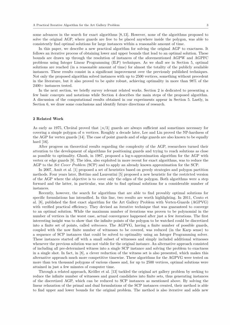
Figures 5, 6 and 7 illustrate the execution of the AGP algorithm on an orthogonal polygon.

Fig. 5 Solving the AGPW (lower bound): The initial witness set D (Chwa-Points) (left); the arrangement Arr(D)and the light AVPs (center); the solution to AGPW(D) (right).


Fig. 6 Solving AGPFC (upper bound): Updated witness set Df (left); the solution to AGPWFC(Df , VL(D)∪V ) andto AGPFC(VL(D) ∪ V ) (right).

Fig. 7 Solving the AGPW (lower bound): The new witness set D (left); the arrangement Arr(D) and the light AVPs(center); the solution to AGPW(D) and to the AGP (right).

5 Computational Results

To report how the experiments, conducted to validate our algorithm, were performed, we describe thecomputing environment, the instances used, the parameters employed and how they affect the overallperformance of the resulting implementation. Lastly, a comparison with other existing techniques ispresented, followed by a summary of the results obtained with all tested instances.

5.1 Computing Environment

All the experiments were performed on standard PCs featuring an Intel R© CoreTM i7-2600 at 3.40 GHz,8 GB of RAM and running GNU/Linux 3.2.0.

Our algorithm (Algorithm 5) was coded in the C++ programming language. The program uses theComputational Geometry Algorithms Library (cgal) [6], version 3.9, to benefit from visibility operations,arrangement constructions and other geometric tasks. To solve the integer programs that model the SCPinstances, we used the xpress Optimization Suite [21], version 7.0.

To achieve accurate time measurements, all tests were run in isolation, i.e., no other process was beingexecuted concomitantly. Moreover, the experiments were run on a single core of the processor, hence, notprofiting from parallelism. Each process was given a time limit of 60 minutes, after which, the instancewas considered unsolved and the program was terminated.


5.2 Instances

In total, our benchmark included more than 2400 publicly available test polygons with and without holes.By collecting such an extended experimentation testbed, from various sources, comprised of polygons ofmultiple classes and sizes, we were able to stress the algorithm robustness.

For polygons without holes, three classes of polygons were used: simple, orthogonal and Von Kochpolygons. The sets of simple polygons were obtained from the work by Bottino et al. [5] (250 polygons)and by Couto et al. [8] (600 polygons).

Random orthogonal polygons included 80 instances from [5] and another 600 instances from [8], whilea third set of hole-free polygons contained 480 Von Koch polygons also from [8].

The instances were grouped according to their source and sizes: those from Bottino et al. containbetween 30 and 60 vertices and are subdivided in groups of 20 polygons each. Those from Couto et al.range from 20 to 2500 vertices and each group has 30 instances of equal size.

In the case of polygons with holes, 120 instances called spike polygons ranging with 60, 100, 200 and500 vertices were obtained from the work by Kröller et al. [13]. As we point out later, the availability ofthese instances afforded us the possibility of comparing our method with the technique presented in [13],which currently is among the most promising methods for solving the AGP.

On the other hand, to make for the lack of diversity of instances with holes in the available benchmarks,we generated another 300 random polygons with holes. These additional instances were made availablein our web page [15] so that they can be used for further comparisons. To construct these new polygonswith holes, two different generation techniques were used, each responsible for producing half of thesenew instances.

To understand the process of generating random simple polygons, picture a randomly generated setof points uniformly distributed inside a given rectangle. cgal’s random_polygon_2 procedure generatesa (not necessarily simple) polygon whose vertices are given by a random permutation of those points andapplies a method of elimination of edge intersections based on 2-opt moves (see [20]).

Now, for the first technique, denoted here GB, the process works as follows: after creating the outerboundary for a random simple polygon with holes, consider that we are left with v vertices to be dis-tributed among h holes. After generating a random uniform partition of v into h parts, we iterativelygenerate the h holes in the following way. At each iteration, we randomly select a point in the interiorof the polygon around which we center an isothetic square entirely contained inside the polygon. Thissquare is then stretched in each of the four orthogonal directions, chosen in random order, by λD whereλ is a stretch factor randomly picked from the interval [0.25, 0.75] and D is the maximum elongationwithin the polygon in that direction. A hole, as a simple polygon, is then created, within this placeholderrectangle, having its number of vertices chosen from one of the unused parts of the previously mentionedrandom partition of v. Here, for an instance with a total of n vertices, n/4 of them were assigned to theouter boundary and 3n/4 of them distributed among n/10 holes.

In contrast, in the second technique, denoted GD, the outer boundary of the polygon as well as allthe holes are random orthogonal polygons. The maximal placeholder rectangle is constructed so that thechosen random interior point c is one of its vertices. Then, at each iteration, besides randomly selectinga new hole size, two holes are allowed to intersect, in which case, they merge into a single hole. Similarlyto the previous generator, for an instance with a total of n vertices, the outer boundary has roughly n/4of them, while the remainder are distributed among the resulting n/10 holes.

The range [100, 500], with step size 100, was used for the number of vertices of the polygons with holes.A total of 30 polygons of each size per generator were produced using these methods, resulting in GBcreating 150 instances (the simple-simple class) and an equal number produced by GD (the ortho-orthoclass).

All instances experimented in Couto et al. and Tozoni et al. work can be found in our project page [15].

5.3 Development History

Since the present work expands and improves our own previous work [18], a comparison of results is due.Let us take, as an example, the polygon in Figure 8, which is a real instance representing a square inBremen, Germany, with 14 holes and 311 vertices taken from [3]. More than 20000 seconds were requiredto obtain an optimal solution using version V1 of our implementation reported in [18].


Subsequent improved versions of the algorithm and its implementation, leading to version V2, in-cluded:

– upgrading the visibility polygon calculation by avoiding computation related to holes that would notbenefit the result;

– cutting short the AGPFC procedure whenever the general upper bound found for the AGP hadthe same cardinality as the current AGPWFC solution, allowing it to skip to the next iteration ofAlgorithm 5.

As an illustration, V2 took less than 10000 seconds to obtain an optimal solution for the aforementionedBremen instance.

Next, by reversing the point of view of visibility testing from the perspective of the guards to thatof the witnesses (fewer in number, in our approach) we avoided computing many visibility polygons andreused those already required for setting up the arrangement. Moreover, by caching visibility informationbased on pairs of points already tested, the performance was further improved. Notice that the ILP matrixconstruction remained the same and changed little on how the algorithm works. This lead to version V3which solved the Bremen instance five times faster than V2.

Recall from Section 4.3 that the ultimate version, V4, of the method described in this work includesthe use of the Lagrangian heuristic for solving the SCP model, besides the removal of lines and columnsfrom the original SCP matrix.

Moreover, V4 takes advantage of reusable information from previous iterations. For instance, if alower bound LB for the AGP instance has been established, Algorithm 2 can be halted when solving anew AGPW(D) instance as soon as a primal solution with cardinality LB is found for the correspondingSCP instance in line 4 (for instance, using the Lagrangian Heuristic). This follows from the fact that LBwas obtained by solving an AGPW(S) instance, for some S ⊂ D. Another interesting situation happenswhen we are solving an AGPWFC instance inside the iterative algorithm for AGPFC (Algorithm 3).Since, in this procedure, witnesses are added and never removed, we can guarantee that the solution ofthe previous AGPWFC instance is a lower bound for the next instance. Using V4, it took less than 600seconds to reach an optimal solution for the Bremen instance!

Fig. 8 Instance representing a square in Bremen, Germany (left); and an optimal guard positioning (right).

5.4 Discretization Techniques for the Witness Set

In Section 4.4, we presented three possible initial discretizations for the witness set. Natural questionsthat arise are: which of these leads to the highest number of exact solutions among multiple classes ofinstances of different sizes? With fewer iterations? With best time performance? Table 1 and Figure 9


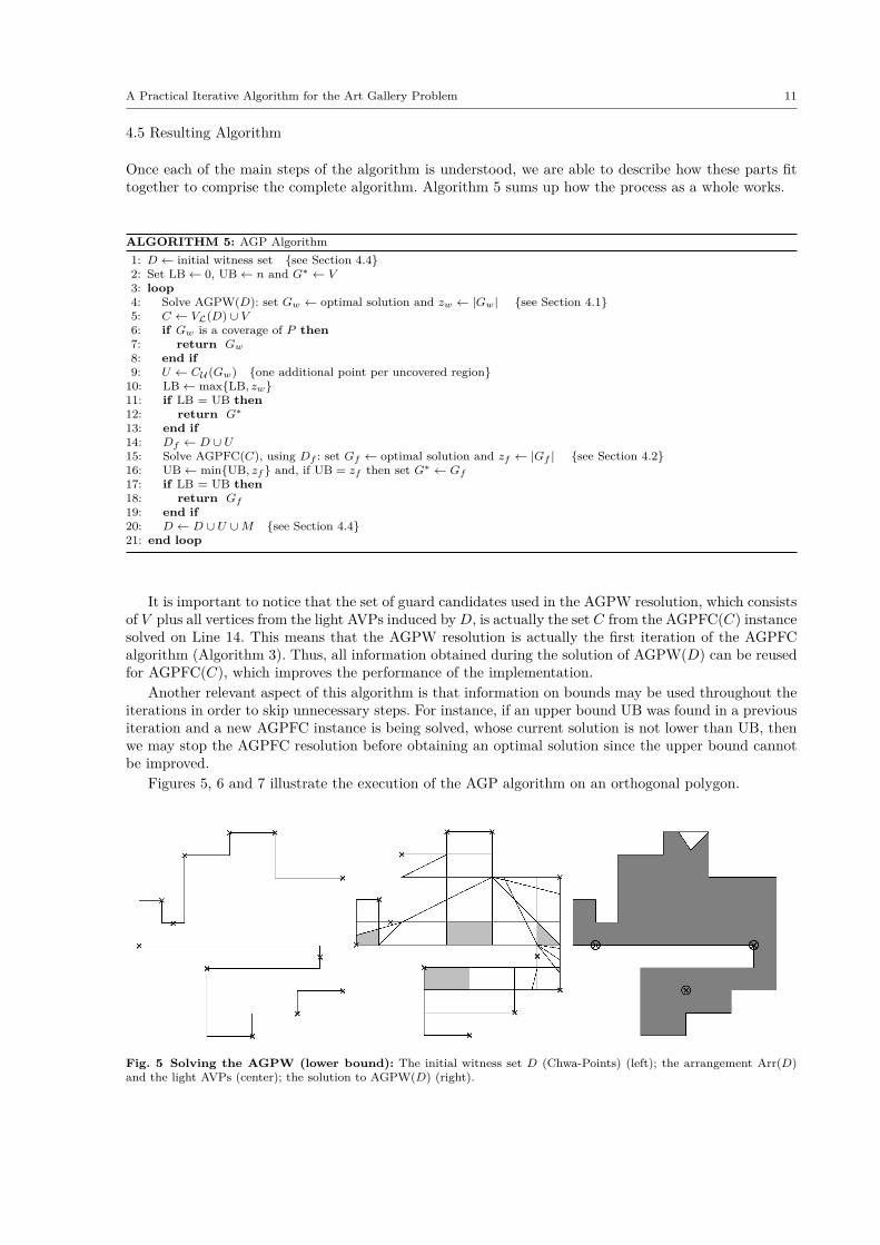
display results obtained in this direction, which exemplify the behavior of the vast majority of the casesobserved. In this summary, only ortho-ortho and simple-simple instances with sizes ranging from 100 to500 vertices were displayed.

Table 1 Number of instances solved to optimality when using each of the three initial discretization techniques

Instance Group n# of Instances Solved

All-Vertices Convex-Vertices Chwa-Points

Simple-simple(30 inst. per size)

100 30 30 30200 30 30 30300 29 30 30400 29 30 28500 26 27 28

Ortho-ortho(30 inst. per size)

100 30 30 30200 29 29 30300 29 29 30400 30 30 30500 27 27 28

Fig. 9 Average number of iterations per size (left); and average time spent per size (right).

In Table 1 we have the number of instances that were solved to optimality using each discretization.As said before, the tests were halted after one hour of execution time. We can see that Chwa-Pointsand Convex-Vertices achieved the best results, solving 294 and 292 of the 300 instances considered,respectively.


By analyzing the charts in Figure 9, which presents the average number of iterations and the averagetime of successful runs, we see a reasonable advantage when using Chwa-Points. In the case of simple-simple polygons with 500 vertices, for example, we have a savings of more than 200 seconds when usingChwa-Points as opposed to Convex-Vertices. If we compare to the All-Vertices technique, this differencegrows to more than 500 seconds, on average.

The graphs for All-Vertices and Convex-Vertices show that while they lead to very similar resultsin regard do the number of iterations, the latter has a considerable advantage over the former in runtime and consequently in the number of instances solved to optimality (Table 1). This behavior stemsfrom the fact that the discretization points in the Convex-Vertices strategy is a subset of the ones in theAll-Vertices and clearly a larger witness set leads to more visibility polygon computations, more complexvisibility arrangements and, consequently, larger SCP instances to be solved.

The Chwa-Points discretization technique, having been the most successful one, was chosen as thestandard initial discretization for our method. In this context, throughout the following sections, allresults presented were obtained using this initial discretization.

5.5 Lagrangian Heuristic

In Section 4.3, the Lagrangian heuristic was presented as a means to reach optimal solutions for AGP-WFC (SCP) instances faster. Lagrangian relaxation is reported (c.f., [2]) to perform well in many SCPapplications and, therefore, we decided to test it on the SCP instances arising in the context of the AGP.In this section, we briefly analyze the pros and cons of using this technique in our implementation. Forthis comparison, four groups of instances, with sizes between 100 and 500, were considered: simple andorthogonal instances from Couto et al. [8] and the new simple-simple and ortho-ortho classes.

Table 2 shows results containing the number of instances solved when using (not using) the heuristic.Since optimal solutions were always found for all hole-free instances (with or without the heuristic),the table only show results for instances from the simple-simple and ortho-ortho classes. From theseresults, we can see that the number of instances solved within our timeframe of one hour did not varyconsiderably. Actually, in the case of the simple-simple group, the version without the heuristic was ableto solve one additional instance.

So, at first glance, it does not seem to be advantageous to employ the Lagrangian heuristic. Never-theless, the time used to compute viable solutions for SCPs using the heuristic is usually negligible withrespect to the time spent in the other parts of our implementation. Besides, some instances benefited fromusing the heuristic and, in general, it yielded good primal bounds for SCP, which was its primary goal.Thus, in an attempt to understand why the optimality rate was not positively affected by the usage ofthe heuristic, we investigated this issue a little further. To this end, we looked at the solutions producedby both the heuristic and the ILP solver xpress for some instances. It turned out that, although theyhad equal sizes, these solutions were often not the same, resulting in different uncovered regions as wellas different witness and guard candidate sets. As a consequence, the next sequence of SCPs to be solvedchanged considerably, deeply affecting the time required to find the optimum of the AGP. This observa-tion shows that more research is needed to distinguish among the optimal SCP solutions those that aremore promising for our algorithm, i.e., that allow it to solve the AGP quicker. For the time being, weturn our attention to the effects of the Lagrangian heuristic in the total running time.

Regarding the average run time when using the Lagrangian heuristic, the graphs in Figure 10 show acomparison for the case of each of the four groups tested. These graphs include only instances that weresolved to optimality regardless of whether the Lagrangian heuristic was used.

In general, we perceive a modest advantage when using the Lagrangian heuristic in our procedure.Therefore, we decided to maintain the usage of the Lagrangian heuristic as the default option in all thetests reported in the following sections.

5.6 Comparison with other State of Art Techniques

Recently, some techniques achieved good practical results in the search for optimal solutions for the AGP.In 2011, Bottino and Laurentini [5] presented a heuristic based on an edge covering algorithm that leadto some nice results, while still not able to achieve optimality for a large set instances. A full comparisonbetween our technique and that heuristic appeared in [18].


Table 2 Number of instances solved to optimality when using or not the Lagrangian Heuristic method

Instance Groups nInstances solved

Without LH With LH

Simple-Simple(30 inst. per size)

100 30 30200 30 30300 30 30400 28 28500 29 28


100 30 30200 30 30300 29 30400 30 30500 29 28

Fig. 10 Comparison between using and not using the Lagrangian heuristic on four different types of polygons.

Through a rather different approach, Kröller et al. [13], in 2012, presented a method that reached opti-mality for many large and complex instances. For the sake of comparison, we also ran our implementationon the same instances used in that paper. Table 3 shows the average running times and optimality ratesof the two methods. In comparing these results, one has to bear in mind the computational environmentsin which the two experiments were conducted were rather different.

It can be seen from Table 3 that our technique reached optimal solutions for all instances within asmall average running time. While we initially allowed a time limit of 60 minutes, as opposed to Kröller etal.’s (see [13]) 20 minute upper bound on the total running time, no more than ten minutes were actuallyrequired for our method to converge in all those instances. As said before, this statistic has to be readwith caution since the computing environments used were not comparable. A deeper look into the timeperformance of our method, however, dismisses the hasty conclusion that this difference might explain its


Table 3 Comparison between the method of Kröller et al. and ours

Instance Group nOptimality Rates Average Time (s)[13] Ours [13] Ours

Simple(30 inst. per size)

60 80% 100% 0.70 0.26100 64% 100% 29.40 0.94200 44% 100% 14.90 3.77500 4% 100% 223.30 35.04

Orthogonal(30 inst. per size)

60 80% 100% 0.40 0.15100 54% 100% 1.10 0.64200 19% 100% 4.30 2.66500 7% 100% 25.30 20.44

Von Koch(30 inst. per size)

60 77% 100% 2.40 0.26100 71% 100% 5.50 0.87200 70% 100% 18.90 6.63500 15% 100% 205.00 76.45

Spike(30 inst. per size)

60 67% 100% 1.70 0.49100 68% 100% 3.90 1.40200 61% 100% 15.30 7.30500 52% 100% 190.20 173.23

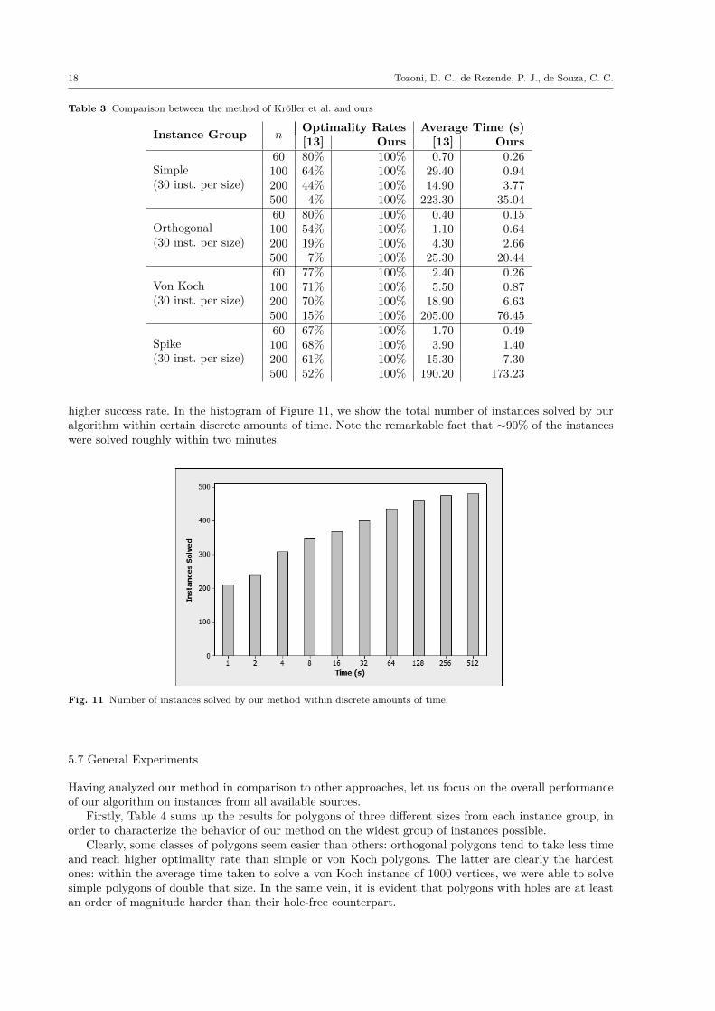
higher success rate. In the histogram of Figure 11, we show the total number of instances solved by ouralgorithm within certain discrete amounts of time. Note the remarkable fact that ∼90% of the instanceswere solved roughly within two minutes.

Fig. 11 Number of instances solved by our method within discrete amounts of time.

5.7 General Experiments

Having analyzed our method in comparison to other approaches, let us focus on the overall performanceof our algorithm on instances from all available sources.

Firstly, Table 4 sums up the results for polygons of three different sizes from each instance group, inorder to characterize the behavior of our method on the widest group of instances possible.

Clearly, some classes of polygons seem easier than others: orthogonal polygons tend to take less timeand reach higher optimality rate than simple or von Koch polygons. The latter are clearly the hardestones: within the average time taken to solve a von Koch instance of 1000 vertices, we were able to solvesimple polygons of double that size. In the same vein, it is evident that polygons with holes are at leastan order of magnitude harder than their hole-free counterpart.


Table 4 Summary of results

Source Instance Group n Optimality Rate Guards Iterations Time (s)

Couto et al.


100 100.00% 13.17 1.93 0.941000 100.00% 126.57 4.50 181.272500 76.67% 312.39 5.78 2349.84


100 100.00% 14.63 2.50 0.641000 100.00% 147.90 5.40 120.292500 100.00% 371.40 6.87 1139.80

Von Koch(30 inst. per size)

100 100.00% 7.83 1.70 0.871000 100.00% 56.80 2.37 723.541500 73.33% 95.00 2.67 2584.83

Bottino andLaurentini


40 100.00% 5.55 1.15 0.1050 100.00% 6.60 1.60 0.2460 100.00% 8.35 1.30 0.27


40 100.00% 6.00 1.40 0.0750 100.00% 7.70 1.55 0.1260 100.00% 9.10 1.50 0.16

Kröller et al. Spikes(30 inst. per size)

100 100.00% 4.37 1.07 1.40200 100.00% 6.87 1.00 7.30500 100.00% 9.77 1.00 173.23

Tozoni et al.

Simple-simple(30 inst. per size)

100 100.00% 13.13 2.27 4.92200 100.00% 24.30 3.47 34.68500 93.33% 59.68 5.82 498.69


100 100.00% 12.27 2.97 7.88200 100.00% 24.97 4.90 45.29500 93.33% 62.46 6.29 433.03

Although average time information can be useful for a general analysis, it is often necessary to observethe behavior on particular instances. In Figure 12, three box-plot charts present the running time resultsfor different classes of polygons. In these charts, it is possible to perceive that the average times (fromTable 4) for a given class and size of polygons may be quite disparate from the median, or even largerthan the third quartile, due to outliers. For instance, consider the Ortho-ortho polygons with 200 vertices:the average time to solve the AGP is 45.29 seconds, while the median and the third quartile are 24.96and 41.38 seconds, respectively. It is clear from these numbers that the instance classes contain polygonswhich differ considerably from each other, leading to AGP instances with very diverse degrees of difficulty.The high success rate of our algorithm in such a heterogeneous benchmark indicates that the method isvery robust.

Quite informative also is an analysis of how the total running time is divided between the differentcomputational tasks, in practice. While one would expect that the larger amount of time should be spentsolving the ILP (SCP) instances, after all these are NP-hard problems, we observe from the histogram inFigure 13 that the time spent solving ILP models is usually lower than half of the total time. This can becredited to the high quality of modern solvers, such as xpress, but, in our case, also to the improvementsmade in our implementation, such as matrix reduction and the Lagrangian heuristic. Of course, were weto consider ever growing instance sizes, this behavior is expected to change, asymptotically.

Needless to say, the amount of time spent in the resolution of ILP models is proportionally larger forinstances with holes as a consequence of the denser and more complex arrangements, which lead to largerand harder ILP instances.

5.8 Implementation

As mentioned earlier, our implementation relies on an ILP solver to quickly solve SCP instances. Initially,our choice was for the xpress Optimization Suite [21] (version 7.0), as a state of the art software capableof finding solutions for very large and complex instances in a matter of minutes. For this reason, allexperiments reported up until now were conducted with xpress.


Fig. 12 Box-plot charts summarizing information about the running times to solve Simple-simple, Ortho-ortho and Spikeinstances.

Fig. 13 Comparison between preprocessing time and solver time for polygons of 500 vertices.

However, as xpress is a proprietary software, we also included in our implementation the possibility ofusing a free ILP solver to facilitate further tests and comparisons of our techniques with new algorithms.The free package of choice was the glpk (GNU Linear Programming Kit) [12], a set of routines writtenin the ANSI C programming language and organized in the form of a callable library. Although switchingto a non-commercial solver is expected to lead to some degradation in performance, it remains a handyand easy to use means for benchmarking future researches on the subject.


As an illustration of the loss of performance, we carried out some extra tests to assess the impactof switching between these two ILP solvers. Table 5 shows the ratio between the time needed to solveinstances of polygons with 1000 vertices when running our code with xpress and with glpk. Fromthese results, we can see a considerable advantage when selecting xpress, at least for simple polygons.Curiously, when we consider orthogonal polygons, glpk presents a modest advantage.

Table 5 Rates between the running times when employing xpress and glpk

ILP Solver Time RateSimple Orthogonal

glpk/xpress 2.56 0.89

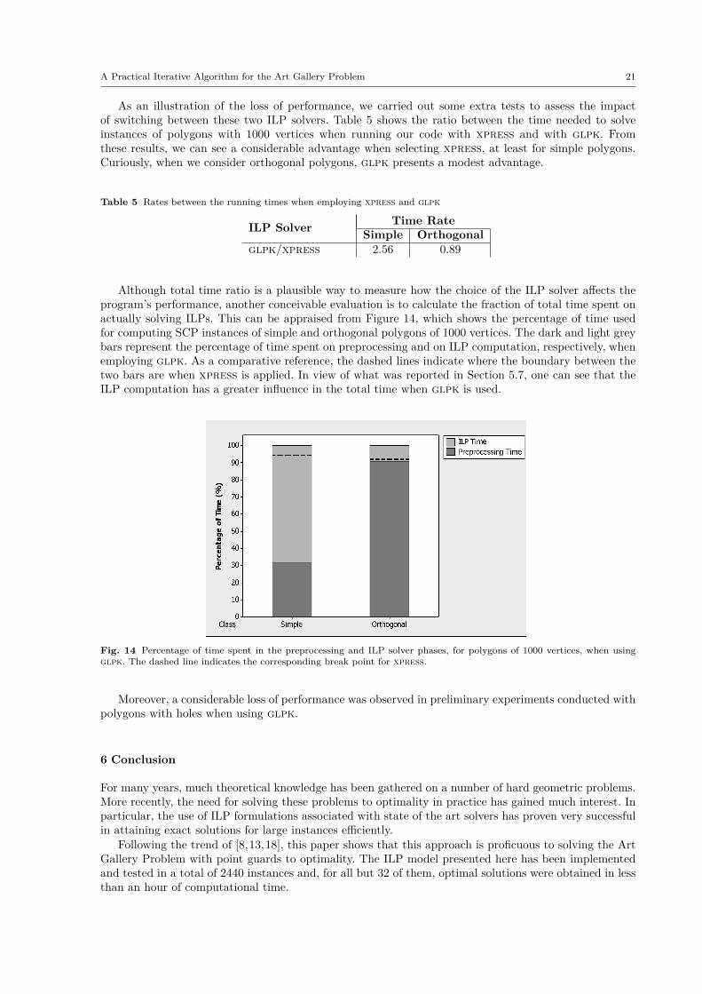
Although total time ratio is a plausible way to measure how the choice of the ILP solver affects theprogram’s performance, another conceivable evaluation is to calculate the fraction of total time spent onactually solving ILPs. This can be appraised from Figure 14, which shows the percentage of time usedfor computing SCP instances of simple and orthogonal polygons of 1000 vertices. The dark and light greybars represent the percentage of time spent on preprocessing and on ILP computation, respectively, whenemploying glpk. As a comparative reference, the dashed lines indicate where the boundary between thetwo bars are when xpress is applied. In view of what was reported in Section 5.7, one can see that theILP computation has a greater influence in the total time when glpk is used.

Fig. 14 Percentage of time spent in the preprocessing and ILP solver phases, for polygons of 1000 vertices, when usingglpk. The dashed line indicates the corresponding break point for xpress.

Moreover, a considerable loss of performance was observed in preliminary experiments conducted withpolygons with holes when using glpk.

6 Conclusion

For many years, much theoretical knowledge has been gathered on a number of hard geometric problems.More recently, the need for solving these problems to optimality in practice has gained much interest. Inparticular, the use of ILP formulations associated with state of the art solvers has proven very successfulin attaining exact solutions for large instances efficiently.

Following the trend of [8,13,18], this paper shows that this approach is proficuous to solving the ArtGallery Problem with point guards to optimality. The ILP model presented here has been implementedand tested in a total of 2440 instances and, for all but 32 of them, optimal solutions were obtained in lessthan an hour of computational time.


While convergence remains dependent on the initial discretization, the current results already showan efficacy rate of more than 98%, which is an achievement unattained up to this point in time.

It remains a challenge for the future to study additional geometric properties that may assist indesigning a discretization strategy that leads to proven convergence of the method described in thiswork.

Along with this paper, we are making the code of our program available to interested researchers andpractitioners. To facilitate its use, we implemented an option for selecting glpk (GNU Linear Program-ming Kit) [12] as the ILP solver used for solving SCPs. As is the case of the required cgal[6] library, glpkalso provides a free license. Therefore, to anyone willing to use our software it will suffice to downloadthose packages and compile the code on the preferred platform.

Although some loss of performance is perceived upon replacement of the commercial solver by glpk,our implementation remains an invaluable tool for those interested in studying the AGP.

To the best of our knowledge, no other robust code that tackles this problem has ever been made acces-sible. Therefore, our aim in doing so is to provide a comparative gauge for reliable evaluation of differentsolution methods for the AGP. The code can be downloaded at www.ic.unicamp.br/∼cid/Problem-ins-tances/Art-Gallery/AGPPG/code/agsol-v1.0.0.tar.gz.

Acknowledgements We would like to thank Alexander Kröller and Sandór Fekete for fruitful discussions and for providingadditional sets of instances for our experiments. We are also grateful to Andrea Bottino for promptly dispensing the instancesused in his work for the tests conducted in our investigation.

References

1. Y. Amit, J. S. B. Mitchell, and E. Packer. Locating guards for visibility coverage of polygons. In ALENEX, pages1–15, New Orleans, Lousiana, January 2007. SIAM.

2. J. E. Beasley. Lagrangian relaxation. In C. R. Reeves, editor, Modern Heuristic Techniques for Combinatorial Problems,pages 243–303. John Wiley & Sons, Inc., New York, NY, USA, 1993.

3. D. Borrmann, P. J. de Rezende, C. C. de Souza, S. P. Fekete, S. Friedrichs, A. Kröller, A. Nüchter, C. Schmidt, andD. C. Tozoni. Point guards and point clouds: solving general art gallery problems. In Proceedings of the twenty-ninthannual symposium on Computational geometry, SoCG ’13, pages 347–348, New York, NY, USA, 2013. ACM.

4. P. Bose, A. Lubiw, and J. I. Munro. Efficient visibility queries in simple polygons. Computational Geometry, 23(3):313–335, 2002.

5. A. Bottino and A. Laurentini. A nearly optimal algorithm for covering the interior of an art gallery. Pattern Recognition,44(5):1048–1056, 2011.

6. CGAL. Computational Geometry Algorithms Library, 2012. www.cgal.org (last access January 2012).7. K.-Y. Chwa, B.-C. Jo, C. Knauer, E. Moet, R. van Oostrum, and C.-S. Shin. Guarding art galleries by guarding

witnesses. Intern. Journal of Computational Geometry And Applications, 16(02n03):205–226, 2006.8. M. C. Couto, P. J. de Rezende, and C. C. de Souza. An exact algorithm for minimizing vertex guards on art galleries.

International Transactions in Operational Research, 18(4):425–448, 2011.9. S. K. Ghosh. Approximation algorithms for art gallery problems. In Proc. Canadian Inform. Process. Soc. Congress,

pages 429–434, Mississauga, Ontario, Canada, 1987. Canadian Information Processing Society.10. S. K. Ghosh. Visibility Algorithms in the Plane. Cambridge University Press, New York, 2007.11. S. K. Ghosh. Approximation algorithms for art gallery problems in polygons. Discrete Applied Mathematics, 158(6):718–

722, 2010.12. GLPK. GNU Linear Programming Kit. GNU, 2013. http://www.gnu.org/software/glpk/ (access December 2013).13. A. Kröller, T. Baumgartner, S. P. Fekete, and C. Schmidt. Exact solutions and bounds for general art gallery problems.

J. Exp. Algorithmics, 17(1):2.3:2.1–2.3:2.23, May 2012.14. D. T. Lee and A. Lin. Computational complexity of art gallery problems. Information Theory, IEEE Transactions on,

32(2):276–282, March 1986.15. D. C. T. M. C. Couto, P. J. de Rezende, and C. C. de Souza. The Art Gallery Problem project (point guards), 2013.

www.ic.unicamp.br/∼cid/Problem-instances/Art-Gallery.16. J. O’Rourke. Art Gallery Theorems and Algorithms. Oxford University Press, New York, NY, 1987.17. T. C. Shermer. Recent results in art galleries. Proceedings of the IEEE, 80(9):1384–1399, September 1992.18. D. C. Tozoni, P. J. de Rezende, and C. C. de Souza. The quest for optimal solutions for the art gallery problem: A

practical iterative algorithm. In V. Bonifaci, C. Demetrescu, and A. Marchetti-Spaccamela, editors, Proceedings of the12th International Symposium on Experimental Algorithms, SEA 2013, volume 7933 of Lecture Notes in ComputerScience, pages 320–336, Rome, Italy, 2013. Springer.

19. J. Urrutia. Art gallery and illumination problems. In J. R. Sack and J. Urrutia, editors, Handbook of ComputationalGeometry, pages 973–1027, Amsterdam, 2000. Elsevier Science Publishers.

20. J. van Leeuwen and A. Schoone. Untangling a traveling salesman tour in the plane. In Proc. 7th Conference onGraph-Theoretic Concepts in Computer Science, pages 87–98, Munich, 1981. Rijksuniversiteit. Vakgroep Informatica.

21. XPRESS. Xpress Optimization Suite. FICO Solutions, 2013. http://www.fico.com/en/products/fico-xpress-optimization-suite/ (access November 2013).

Date post:	15-May-2018
Category:	Documents
Upload:	nguyendat
View:	223 times
Download:	1 times

A Practical Iterative Algorithm for the Art Gallery ... · A Practical Iterative Algorithm for the...

Documents