A primer on turbulence in hydrology and hydraulics: The powerof dimensional analysis
Gabriel Katul1 | Dan Li2 | Costantino Manes3
1Nicholas School of the Environment, DukeUniversity, Durham, North Carolina2Department of Earth and Environment, BostonUniversity, Boston, Massachusetts3DIATI—Department of Environment, Land andInfrastructure Engineering, Torino, Italy
Correspondence Gabriel Katul, Nicholas Schoolof the Environment, Duke University, Durham,NC 27708.Email: [email protected]
Funding informationArmy Research Office, Grant/Award Number:W911NF-18-1-0360; Compagnia di San Paolo,Grant/Award Number: Attrarre Docenti di Qualittramite Starting Grant; Division of Atmosphericand Geospace Sciences, Grant/Award Number:NSF-AGS-1644382; Division of Earth Sciences,Grant/Award Number: NSF-EAR-1344703;Division of Integrative Organismal Systems, Grant/Award Number: NSF-IOS-1754893
The apparent random swirling motion of water is labeled “turbulence,” which is apervasive state of the flow in many hydrological and hydraulic transport phenom-ena. Water flow in a turbulent state can be described by the momentum conserva-tion equations known as the Navier–Stokes (NS) equations. Solving theseequations numerically or in some approximated form remains a daunting task inapplications involving natural systems thereby prompting interest in alternativeapproaches. The apparent randomness of swirling motion encodes order that maybe profitably used to describe water movement in natural systems. The goal of thisprimer is to illustrate the use of a technique that links aspects of this ordered stateto conveyance and transport laws. This technique is “dimensional analysis”, whichcan unpack much of the complications associated with turbulence into surprisinglysimplified expressions. The use of this technique to describing water movement instreams as well as water vapor movement in the atmosphere is featured. Particularattention is paid to bulk expressions that have received support from a large bodyof experiments such as flow-resistance formulae, the Prandtl-von Karman log-lawdescribing the mean velocity shape, Monin-Obukhov similarity theory that correctsthe mean velocity shape for thermal stratification, and evaporation from rough sur-faces. These applications illustrate how dimensional analysis offers a pragmaticapproach to problem solving in sciences and engineering.
Hydrology and hydraulics are primarily concerned with water movement in liquid or vapor phases within natural(e.g., watersheds, wetlands and marshes, atmosphere) or engineered (e.g., pipes, ducts, channels, spillways) systems. In manyinstances, the water movement appears to be dominated by complex swirling or eddying motion that is labeled “turbulence.”It is a flow state, not a fluid property, that is commonly contrasted with the simpler “laminar” flow state. At the microscopiclevel, the occurrence of turbulence may superficially appear to violate the second law of thermodynamics. How can so manywater molecules spontaneously start to move almost coherently together in a large swirl or plume within eddies instead of fol-lowing their random (or Brownian) motion trajectory predicted by the kinetic theory? The answer to this question is at theheart of turbulence research and has numerous consequences in a plethora of sciences. Flow organization by the swirling oreddying motion at some spatial scales leads to enhanced overall dissipation of energy (a conversion of kinetic energy to heatper unit time) by the action of viscosity (or internal friction in fluids), thus ensuring maximum entropy production. This asser-tion implies that order or coherency may be needed in certain regions of the flow domain to increase overall disorder orentropy in the entire flow domain. At the macroscopic (or continuum) level, water flow in a turbulent state can be described
Received: 18 September 2018 Revised: 26 November 2018 Accepted: 12 December 2018
by the momentum conservation equations, which are known as the Navier–Stokes (NS) equations. The NS equations havebeen derived to account for the effects of viscosity in fluids thereby marking a major departure from the so-called Euler equa-tions for ideal or frictionless fluids. The mathematical properties of the NS equations (existence of solutions and smoothness)continue to be one of the important open problems in mathematics as declared by the Clay Mathematics Institute. The NSequations, being equations describing fluid velocity in time at a given position, tend to “hide” the numerous scales involved inenergy transfer and dissipation by viscosity. Numerical integration of the NS equations or some approximated version of themhas been one of the drivers in the creation of a new branch in science known as computational fluid dynamics (CFD). CFDlead to remarkable developments in both computer hardware and an impressive suite of numerical algorithms for solving NS(Pope, 2000) or a more fundamental version of them routed in molecular dynamics (Succi, 2001). Simulations have come longways since Lewis Fry Richardson first attempted numerical weather predictions (Richardson, 1922). While Richardson's simu-lations failed to provide superior weather predictions, they did spawn novel ideas about turbulence representation and werepartly responsible for the discovery of chaos in weather (Lorenz, 1963). High-performance computing and CFD have now suf-ficiently matured to a point they are beginning to replace expensive laboratory experiments and field-scale testing in numerousbranches of engineering. As early as 1949, von Neumann envisioned that supercomputers can help unravel the “mysteries” ofturbulence. While mainly used for research purposes, direct numerical simulations (DNS) of the NS equations that utilize avariety of brute-force numerical integration techniques are conducted to visualize the intricate flow patterns created by turbu-lence. At first glance, the DNS results may seem highly chaotic but actually hide a great deal of coherency. In the meantime,experimental facilities and instrumentation development as well as fast imaging techniques are allowing exploration and visu-alization of turbulence in ways not imaginable 20 years ago. In fact, modern flumes, pipes, and wind tunnel facilities are a tes-tament to the rapid progress made when referenced to the early facilities of O. Reynolds (in 1883) and L. Prandtl (in 1904).
Progress on turbulence theories have not experienced the rapid developments witnessed in simulations and experiments. Itis now becoming a cliche to recite a long list of famed engineers, mathematicians, and physicists (e.g., Boussinesq, Feynman,Heisenberg, Kolmogorov, Kraichnan, Landau, Per-Bak, Prandtl, Taylor, von-Karman) who worked on turbulence withoutoffering the same successes achieved in their respective fields. Practitioners and engineers have recognized that finite viscositymarks a major departure from Euler's equations and subsequently developed a suite of experiments and tactics to describe tur-bulent flows. In fact, hydraulics was born because of operational needs to describe water flow in situations not addressed byearly hydrodynamics that primarily dealt with the mathematics of frictionless fluids. Thus, around the turn from the 19th tothe 20th century onwards, a large number of semiempirical formulae have been independently introduced to describe turbulentflow properties in hydraulics, hydrology, sediment transport, and meteorology. These formulae remain the corner stone oftextbooks and working professional tool-kits alike (Brutsaert, 2005; French, 1985; Willcocks & Holt, 1899). Their success atpacking a large body of experiments dealing with flow conveyance in pipes and channels as well as momentum and scalarmixing in stratified boundary layers, explains their wide usage in hydraulics, atmospheric, and climate models today. Theycontinue to serve as “work-horse” equations for flow and transport in natural systems operating at Reynolds numbers that aresimply too large for DNS. Arriving at these equations from dimensional considerations is the main goal of this primer. Theapproaches taken here bypass the need to use or solve explicitly the NS equations yet the outcomes they offer do not contra-dict the NS equations. Dimensional analysis also offers an efficient way to plan and execute experiments that unfold generallaws in situations where the laws cannot be derived from first principles. They are the most effective and pragmaticdimension-reduction technique (a technique that reduces a system of differential equations into fewer equations by preservingdesirable features of their phase space) invented in science.
2 | WHAT IS TURBULENCE?
Technically, there is no precise definition of turbulence and only defining syndromes are identified to distinguish turbulencefrom other flows characterized by fluctuating changes in pressure and velocity (such as nonlinear waves). These defining syn-dromes must be simultaneously satisfied and include (Tennekes & Lumley, 1972):
1. Irregularity: Turbulent flows are sufficiently irregular that they make a purely deterministic treatment impossible (theoreti-cally and experimentally). An example of this irregularity is shown in Figure 1 featuring water velocity measurementsabove a smooth channel bed in a flume and atmospheric velocity measurements above a grass-covered surface describedelsewhere (G. Katul & Chu, 1998; G. Katul, Hsieh, & Sigmon, 1997).The causes of this irregularity is often attributed tosensitivity to initial conditions—meaning a small change in initial conditions gets amplified through the nonlinear termsin the NS equations. This amplification leads to differing detailed temporal patterns in any realization of a flow variable ata point despite similarities in the flow configuration. However, the statistics of the flow variables associated with the sameflow configuration represented by the flow realizations remain the same. For this reason, describing turbulence is akin to
2 of 17 KATUL ET AL.
describing the statistics of the flow variables as those appear to be “conserved” across repeated experiments with similarinitial and boundary conditions. A highly simplified system illustrating the properties of such irregularity is the well-studied logistic map. The logistic map is defined as a recurrence relation (i.e., linking the variable at one time step in thefuture to the state of the variable in the present state) with a second-order nonlinearity and is archetypal of how chaoticbehavior arises from a single nonlinear difference equation. It is used here to show (a) the chaotic nature of instantaneoussolutions and (b) the preservation of statistics across similar initial conditions. The NS equations and the logistic map(u(t + 1) = −2u(t)2 + 1) can be expressed, respectively, as (Frisch, 1995)
∂Ui
∂t¼ −Uj
∂Ui
∂xj+
∂τij∂xj
+ Bf i, ð1Þ
u t + 1ð Þ− u tð Þ ¼ − 2u tð Þ2 − u tð Þ + 1, ð2Þ
where Ui = U1, U2, U3 are the instantaneous three velocity components that can also be interpreted as momentum per unitmass of fluid in direction xi, xi = x1, x2, x3 are Cartesian coordinates, t is time, τij are the overall viscous stresses and pressureP acting on a fluid surface given by
τij ¼ ν∂Ui
∂xj+
∂Uj
∂xi
� �−Pδij, ð3Þ
and ν is the kinematic viscosity, δij = 1 when i = j but is zero otherwise (the Kronecker delta), and Bfi is an external force.Repeated subscript j implies summation from j = 1 to j = 3. The logistic map as arranged above shares the following withNS: (a) a velocity difference term (first term on the left-hand side) in time (u(t + 1) − u(t)) approximating the local accelera-tion ∂Ui/∂t, (b) a second-order nonlinear term (first term on the right-hand side), and (c) a term (u(t)) resembling a linearstress–strain expected from Newton's viscosity law for τij (second term on the right-hand side), and a constant body force(Bfi = 1) acting on the fluid (last term on the right-hand side). Figure 2 shows two solutions of the logistic equation deter-mined by perturbing the initial condition u(0) = 0.1 with a small increment = 0.00001. After a certain period (only 100 stepsshown), the two solutions diverge in time but their statistics, as quantified by the histogram or probability density function(PDF), remain the same.
2. Diffusivity: Turbulent flows are diffusive and efficient at transporting heat, mass, and momentum—at least when com-pared with their laminar counterparts.
3. Large Reynolds number: A large Reynolds number Re is necessary to ensure a turbulent flow state so that the aforemen-tioned nonlinear inertia term (or advective acceleration term) in the NS equations far exceeds its viscous counterpart. Thesignificance of this term is the main cause of irregularity as shown earlier. Formally and through a scaling argumentapplied to velocity gradients,
Time (s)
12
14
16
18
20
22
24
26
u(t
)(cm
s–1 )
0 5 10 15 20 150 155 160 165 170 175 180
Time (s)
1
1.5
2
2.5
3
u(t
)(m
s–1 )
FIGURE 1 Measured longitudinal velocity time series u(t) at z = 1 cm above a smooth open channel showing irregularity in turbulence (left). Themeasurements were sampled at 100 Hz when the water depth attained a uniform value of h = 10 cm. Measured u(t) in the atmosphere at z = 5 m above agrass field (right) again illustrating similar irregularity to those reported in the smooth open channel flow. The measurements were sampled at 56 Hz duringdaytime conditions
KATUL ET AL. 3 of 17
Re ¼Uj
∂Ui∂xj
��� ���ν ∂2Ui
∂xj∂xj
� � � Ulν
if j Ui j� U;∂Ui
∂xj� U
l;∂2Ui
∂xj∂xj� U
l2: ð4Þ
Naturally, a transition from laminar (regular) to turbulent (irregular) flow occurs due to the growth of unstable modes thatbecome energized and amplified by the nonlinear advective acceleration term (Drazin & Reid, 2004). The exact details of thetransition to turbulence with increasing Re remains a subject of active research that is beyond the scope of this primer. Severalhighlights have been documented by an editorial in Nature Physics (Pomeau, 2016) as well as the influential and best-sellingbook on chaos (Gleick, 2011).
4. Three-dimensional vorticity fluctuations: This defining syndrome guarantees that turbulence is rotational and three dimen-sional. An important mechanism sustaining such vorticity fluctuation is vortex stretching originating from interactionsbetween turbulent velocity and vorticity. Conservation of angular momentum requires that lengthening of vortices inthree-dimensional fluid flow (vortex stretching) correspond to increases in the component of vorticity in the stretchingdirection. Vortex compression also occurs in turbulent flows. DNS has shown that while both stretching and compressionoccur, vortex stretching occurs more frequently (Pope, 2000). This velocity–vorticity interaction arises again from theadvective acceleration term, which is quite large at high Re. Vortex stretching or compression is entirely absent in two-dimensional flows such as waves.
5. Dissipation and energy cascade: This defining mechanism distinguishes the energetics associated with the NS equationsfrom the Euler equations. Viscous stresses always oppose velocity changes thereby acting to increase the internal energyof the fluid at the expense of kinetic energy of turbulence, also known as turbulent kinetic energy (TKE). In a nutshell, tur-bulence requires an external supply of energy that may be mechanical in nature (e.g., stirring, gravitational, or pressuregradients) or buoyant (as may be the case in convection or density gradients). Part of the external energy supply is used togenerate pressure and velocity fluctuations over a wide range of time and spatial scales (i.e., TKE). Vortex stretching isthen the main mechanism responsible for transferring TKE from large to small scales until it is dissipated into heat by fric-tional forces promoted by viscosity. Such kinetic energy loss rate is referred to as TKE dissipation rate or ϵ.A Reynolds number Re can also be formulated to signify scale-wise separation between length scales where turbulence isproduced (also referred to as integral scales LI) and length scales where turbulence is dissipated by the action of viscosityand is referred to as the Kolmogorov microscale η. It is commonly assumed (Tennekes & Lumley, 1972) that the amountof TKE (=σ2e ) produced at LI is roughly balanced by the amount of kinetic energy dissipated at η. Hence, the productionof TKE must scale as σ3e=LI � ϵ. The eddy sizes where the viscous dissipation rate occurs must include ν and ϵ and thusmust scale as η = (ν3/ϵ)1/4. Combining these two findings results in LI=ηeReαt where α = 3/4 and Ret = σeLI/ν is a Reyn-olds number formed from turbulent quantities. A high Ret results in large separation between scales at which TKE is pro-duced (i.e., LI) and scales at which it is dissipated by the action of viscosity (i.e., η).On the topic of finite dissipation,another contrast to the Euler equations is the time irreversibility of NS. Time reversibility of equations of motion are oftenanalyzed by substituting t with −t and U with −U (i.e., when reversing time, the velocity also reverses direction). For NS,the effect of this substitution can be traced through the following terms:
Time
–1
–0.5
0
0.5
1
u(t
)
u(t+1)= –2 u(t)2+1: u(0)=0.1, u(0)=0.10001
0 20 40 60 80 100 –1 –0.5 0 0.5 1u(t)
10–1
100
101
PD
F(u
)
FIGURE 2 Two solutions for the logistic map differing only by a small perturbation in initial conditions (left). The histogram or probability density function(PDF) for the two solutions are also compared (right). Despite the differences in the temporal dynamics of the two solutions, their statistics (i.e., PDF) arevirtually the same. These are the reasons why turbulence, which abides by Navier–Stokes (NS), is treated in a statistical manner
4 of 17 KATUL ET AL.
∂ −Uið Þ∂ − tð Þ ¼ ∂Ui
∂t, Time reversibleð Þ, ð5Þ
−Uj∂ −Uið Þ
∂xj¼ Uj
∂Ui
∂xj, Time reversibleð Þ, ð6Þ
−∂P∂xi
¼ −∂P∂xi
, Time reversibleð Þ, ð7Þ
ν∂ −Uið Þ
∂xj+
∂ −Uj� �∂xi
� �¼ − ν
∂Ui
∂xj+
∂Uj
∂xi
� �, Time irreversibleð Þ: ð8Þ
Hence, the analysis here suggests that the viscous term delineating ideal (ν = 0) from real (ν > 0) fluids is one of the rea-sons why NS are time irreversible. Another reason is the chaotic nature of the flow that is conceptually similar to the determin-istic chaos encountered in the logistic equation. Any slight variability in the description of Ui(to) at a future time to results intime irreversibility. In chaotic systems, small variations amplify with the progression of time whether time is marching for-ward or backward. The NS and the Euler equations share this chaotic feature. Clearly, irregularity and time irreversibility arelinked in NS despite the fact that the nonlinear advective acceleration term itself is time reversible.
6. Continuum: Turbulence is assumed to abide by the continuum assumption, meaning that fluid and flow properties such asdensity, temperature, pressure, viscosity, velocity, or energy can be defined at a “point.” The term “point” here deviatesfrom the conventional mathematical definition of a sphere with zero radius. In the continuum assumption, a “point” refersto a small volume whose radius is sufficiently large to encompass numerous molecules so that all fluid properties do notvary with variations in the size of the sphere. In turn, this radius must be sufficiently small to capture all the relevant gradi-ents of flow properties. This assumption allows turbulence to be represented by the NS equations at a point alreadyused here.
To sum up, the NS equations are the fluid-flow analog to Newton's second law in solid mechanics (F = ma, F is the netforce imbalance acting on a solid object of mass m and a is its acceleration). Solving for the flow given by NS (i.e., Ui orsome statistic of it) requires knowledge of the forces moving the fluid (e.g., pressure gradient, gravitational potential,etc...), the key fluid property needed to describe resistance to flow, geometric constraints on the flow such as the flowdomain dimensions, and boundary conditions (e.g., roughness properties of the surface). Dimensional analysis takes fulladvantage of these basic ingredients to formulate plausible (i.e., dimensionally consistent) form of the solution to NS with-out actually solving the NS.
3 | DIMENSIONAL ANALYSIS
3.1 | Overview
J.W. Strutt, later known as Lord Rayleigh, prefaced his 1915 work on the principle of similitude (i.e., dimensional analy-sis) with this paragraph (Rayleigh, 1915): “I have often been impressed with the scanty attention paid even by originalworkers to the great principle of similitude. It happens not infrequently that results in the form of laws are put forth asnovelties on the basis of elaborate experiments, which might have been predicted a priori after a few minutes of consider-ation”. By no means is Lord Rayleigh the first to propose the use of dimensional analysis. In fact Galileo used the princi-ple of similitude some 300 years earlier to reason that animals that grow in size while keeping the same shape cannotgrow indefinitely (D'arcy, 1915). Galileo's argument rests on the fact that growth in weight scales as some l3 (assumingconstant density), whereas growth in strength must be related to some cross-sectional area transmitting forces, and thusmust increase as l2. This argument leads Galileo to conclude that the animal strength-to-weight ratio changes in proportionto l−1, where l is some characteristic dimension most impacted by growth. Hence, larger animals have smaller strength-to-weight ratio. This argument would be rather difficult to envision without the power of dimensional analysis(Lemons, 2018).
So, what is dimensional analysis and how to implement it in the studies of turbulence in hydraulics and hydrology? Con-veyance and transport laws describing turbulent flows must arrive at relations among physical variables that have dimensionsof fluid mass [M], length [L], time [T], temperature [K] or scalar concentration [C]. Ideally, these relations must be derivedfrom the NS equations, which remain elusive. Dimensional analysis attempts to arrive at those relations from the point of viewof dimensional consistency (or homogeneity) supplemented by a fundamental theorem (Buckingham, 1914): the Buckingham
KATUL ET AL. 5 of 17
π theorem (BPT). In the applications of dimensional analysis, identifying all the variables impacting the sought quantity is themost challenging step. As earlier noted, the variables to be selected must include (a) constraints on the flow such as geometricconstraints (i.e., domain size or other restrictive dimensions, distance from boundaries), (b) boundary conditions(e.g., roughness element size, surface heating, surface water vapor concentration), (c) fluid properties (e.g., density ρ, dynamicviscosity μ, or kinematic viscosity ν) usually needed to quantify internal resistance to flow, and (d) external forcing drivingthe flow (e.g., pressure gradients, gravitational potentials). Once the list of variables is identified, the BPT can be implementedthrough the following steps: First, the number of dimensionless groups (= Md − Nd) is determined based on the number ofvariables listed (= Md) and the number of independent units involved (= Nd). Second, the dimensionless groups (labeled as π)are formed based on the choice of repeat variables (also set to = Nd) and dimensional homogeneity. Third, one dimensionlessgroup describing the flow variable of interest is written as a function of all the other dimensionless π groups usually in theform π1 = f(π2, π3, ..). The functional form of f(.) needs to be determined experimentally. Occasionally, exploring limitingcases allows some aspects of the functional form of f(.) to be partly unraveled. This tactic requires one of the π groups toapproach zero or infinity thereby ensuring its overall contribution to f(.) is a finite constant multiplier provided the remainingπ groups are not small (Barenblatt, 1996). This approach is now illustrated through examples that are further discussed in thefuture reading section where the functional form of f(.) may be derived from phenomenological theories. None of the formulaeconsidered here has been directly derived from the NS equations. However, a growing number of studies that use results fromDNS confirm that the expressions considered here are not inconsistent with the NS equations.
3.1.1 | Example 1: The Chezy equation and Manning's formula
One of the basic equations in stream or open channel flow links the flux of water (defined as the flow rate Q per unit areaA normal to the flow direction) to the hydraulic radius Rh = A/Pw (Pw is the wetted perimeter), the bed slope So, and a so-called empirical roughness coefficient. This equation is named after Antoine de Chezy (Chézy, 1775) and is considered themost lasting resistance formula to be derived from experiments.
To illustrate, consider a prismatic channel of length Lc characterized by a hydraulic radius Rh and surface roughnessheight r as shown in Figure 3. The hydraulic radius Rh is defined as the ratio of the cross-sectional area (= Bh) to thewetted perimeter (B + 2 h). For a wide channel, h/B < < 1 and Rh = h/(1 + 2 h/B) ≈ h. The roughness measure r maybe related (but not equal) to the mean height of the protruding roughness elements distributed along the channel bed andits sides. Because the flow is assumed to be steady and uniform, the bulk (or area-averaged) velocity is equivalent to thewater flux so that V = Q/A. This is the desired variable to be derived from dimensional considerations here. For this flowand channel geometry, Newton's second law can be used to link the driving force for water movement and the frictionalresistance formed by a surface shear stress τo and the overall area over which this frictional stress acts. For small angle θsuch that So ≈ sin(θ) ≈ tan(θ), the force driving the flow down slope is, as noted in Figure 3, the weight of the wateralong the channel slope direction. Hence, the gravitational driving force is Fg = mg sin(θ), where m is the fluid mass inthe control volume (= LcBh) and is given as ρLcBh. The forces opposing Fg are side (= 2τo(Lch)) and bed (= τo(BLc))frictional forces assumed to originate from the same frictional stress τo. For a steady and uniform (i.e., nonaccelerating)flow, the force balance yields
h
So = tan (θ)
B
θ
Fg = m g So
Bed τo
Side τo
The roughness
elements
characterized by
r and are
uniformly
distributed on
the bed and
channel sides
Lc
Gravitationalforce driving
the flow:
FIGURE 3 A uniform rectangular channel characterized by water depth h, width B, length Lc, slope So, and surface roughness characterized by a protrusionheight r into the flow. The bed and one of the side stresses resisting the flow τo are shown along with the gravitational force Fg driving the flow along So
Hence, the frictional stress τo can be uniquely determined from Rh, ρ, and gSo. As noted earlier, the dimensional analysishere seeks to derive an expression for the desired variable V from the flow conditions and channel geometry. Because τo is aderived quantity, it need not be used in the analysis as an independent variable. To arrive at a list of variables impactingV from the most primitive variables, the following choices are made:
1. Rh for flow constraints,2. r for boundary conditions at the channel bottom and side,3. ρ and μ for fluid properties that are routinely combined to define a kinematic viscosity ν = μ/ρ (also emerges in the vis-
cous stress of the NS), and4. gSo for external forcing derived from the gravitational component driving the flow downslope, where g is the gravitational
constant (and is connected to Bfi in NS).
Hence, V = f(Rh, r, ν, gSo), where f(.) is an unknown function. Again, τo is not included in this list of variables given itscomplete dependence on ρ, g, So, and Rh that are all included in f(.).
The application of the BPT proceeds as follows: Determine the
1. number of variables Md(= 5) (V, Rh, r, ν, gSo).2. number of units involved Nd(= 2). Only [L], [T] are selected as [M] has been eliminated by the choice of ν instead of μ and ρ.3. number of dimensionless (or π) groups required: Md − Nd = 5–2 = 3.4. repeating variables (= Nd = 2) to be common to all the dimensionless groups. It is convenient here to choose the repeating
variables as forcing (= gSo) and geometric constraint (=Rh). The choice of So and Rh is based on experimental pragmatismbecause they are convenient to measure when compared to other variables such as r.
Hence, based on the BPT, the three π groups with gSo and Rh as repeating variables are:
π1 ¼ V gSoð Þa1 Rhð Þa2 ;π2 ¼ r gSoð Þa3 Rhð Þa4 ;π3 ¼ ν gSoð Þa5 Rhð Þa6 : ð11ÞDetermining a1 and a2 for π1 proceeds as follows: noting that the dimensions of V = [L][T]−1, gSo = [L][T]−2, and Rh =
[L] and that π1 must be dimensionless results in the following algebraic equations:
Hence, a1 = −1/2 and a2 = −1 − a1 = −1 + 1/2 = −1/2. Repeating for π2 and π3 leads to a3 = 0 and a4 = −1, anda5 = −3/2 and a6 = −1/2. That is, π1 = f1(π2, π3) yields
VffiffiffiffiffiffiffiffiffiffiffiffigSoRh
p ¼ f 1rRh
,ν
RhffiffiffiffiffiffiffiffiffiffigSoh
p !: ð13Þ
This expression is a relation between a Froude number Fr ¼ V=ffiffiffiffiffiffiffiffiffiffiffiffigSoRh
p, the relative roughness height r/Rh, and a certain
type of bulk Reynolds number formed by ReF ¼ RhffiffiffiffiffiffiffiffiffiffiffiffigSoRh
pð Þ=ν or Fr = f1(r/Rh, ReF). The Froude number is a dimensionlessnumber defined by the ratio of the flow inertia to an external field (i.e., the gravitational field along the flow direction in theopen channel flow here). The Reynolds number is expressed as UoL/ν, where Uo is a characteristic velocity (¼ ffiffiffiffiffiffiffiffiffiffiffiffi
gSoRhp
here),L is a characteristic length (= Rh here), and ν is the kinematic viscosity of water as before. The conventional or text-book ver-sion of the Chezy formula can now be stated as (Keulegan, 1938):
V ¼ ChffiffiffiffiffiRh
p ffiffiffiffiffiffiffigSo
p, ð14Þ
where Ch is the Chezy roughness coefficient and must vary as Ch = f1(r/Rh, ReF). Dimensional analysis is unable to fullydetermine f1(.) necessitating its determination via experiments. However, in the limit of high ReF, it is expected that Ch
becomes independent of Re− 1F ð! 0), a state referred to as fully rough because the roughness elements protrude well above the
viscous sublayer (a thin layer of fluid in direct proximity of the roughness elements, where the fluid flows in a laminar state;see next section) thereby simplifying the expression for Ch to be dependent only on r/Rh. Experiments in fully rough pipesand channels suggest a Ch � (r/Rh)
−1/6 over some range of r/Rh (but not all), where the −1/6 exponent is commonly referredto as the Strickler scaling whose origin and connection to other aspects of turbulence are discussed elsewhere (Bonetti,
KATUL ET AL. 7 of 17
Manoli, Manes, Porporato, & Katul, 2017; Gioia & Bombardelli, 2002). When this experimental result for Ch is combinedwith the Chezy equation,
with n � g−1/2r1/6 (Manning, 1891). For historical reasons, Equation 15 is not used thereby making published values ofn dimensional (Chow, 1959). This section commenced with an estimate of τo from Newton's second law, which is now usedto provide an interpretation of Ch. Equation 17 can be written as
V2
RhgSo¼ V2
τo=ρ¼ V2
u2*¼ C2
h, ð17Þ
where u* = (τo/ρ)1/2 is the so-called friction (or shear) velocity defining a kinematic stress. This outcome shows that squared
Chezy coefficient may be interpreted as an inverse drag coefficient thereby completing the sought result.
3.1.2 | Example 2: The law of the wall
While the previous section considered the bulk velocity V, the focus now is on the shape of the mean velocity profile u(z),
where z is the distance from the boundary and V ≈ 1=hð ÞÐ h0 u zð Þdz.Figure 4 shows the flow configuration associated with this example. In this case, the variable describing the geometric constraint
on the flow is z, the boundary condition remains r, the most relevant fluid property is, as before ν characterizing internal friction,and the forcing is now surrogated to the wall stress τo. As earlier noted, this frictional stress arises to counter any driving forces asearlier encountered in the Manning–Chezy formula in uniform open channel flows. Also, as noted earlier in the interpretation of Ch,τo can be normalized by ρ so that kinematic units are used for stresses thereby eliminating [M]. The quantity u2* ¼ τo=ρ, thesquared friction velocity earlier defined, must be viewed here as a kinematic representation of the surface stress that dependson the external driving force and a fluid property. Dimensional analysis is now used to explore the function f(.) in
dudz
¼ f z, r, ν, u*ð Þ: ð18Þ
As before, Md = 5 and Nd = 2 necessitating three π groups. Repeating variables are selected as z and u* representing, onceagain, the constraint and the forcing. The three π groups are:
π1 ¼ dudz
ua1* za2 ;π2 ¼ rua3* z
a4 ;π3 ¼ νua5* za6 : ð19Þ
u(z)
z
zo r
dudz
= f(z,τo,ρ)
z
Fluid density: ρ
τo
FIGURE 4 The variables impacting the mean velocity gradient du/dz. These include the height from the ground z, and the kinematic surface stress
u* ¼ffiffiffiffiffiffiffiffiffiτo=ρ
p. As z increases, du/dz visually decreases. Also, in the limit of τo = 0, du/dz = 0. Because τo is determined from a balance between frictional
forces resisting the driving forces to ensure no acceleration, a τo = 0 either implies no forcing (i.e., the flow is not moving) or a “free slip” condition. In thefree slip condition, the flow no longer senses the presence of the surface and the velocity is finite at the surface
8 of 17 KATUL ET AL.
The dimensions of du/dz is [T]−1, u* is [L][T]−1, r is [L], and ν is [L]2[T]−1. Those dimensions are now used to determine
a1....a6. For example,
π1 ¼ T½ �− 1 L½ � T½ �− 1� �a1
L½ �a2 ;− a1 − 1 ¼ 0;a1 + a2 ¼ 0, ð20Þ
resulting in a1 = −1 and a2 = 1. Again, repeating this procedure to π2 and π3 yields a3 = 0, a4 = −1, a5 = −1, and a6 = −1.The dimensionless π groups are now expressed as:
π1 ¼ dudz
zu*
; π2 ¼ rz; π3 ¼ u*z
ν
� �− 1: ð21Þ
Hence,
dudz
zu*
¼ frz,
1Re +
� �: ð22Þ
Again, π3 is related to a Reynolds number Re+ = u*z/ν and π2 resembles a local relative roughness. If Re+−1 is sufficiently
small (<< 1) and the goal is to evaluate du/dz far from the wall boundary (i.e., r/z < < 1), then f(π2, π3) becomes independentof both π2 and π3 as these variables must saturate to some constant with Re+
−1, r/z ! 0. Hence, f(.) must be a constant farfrom the boundary and at large Re+. That is,
dudz
zu*
¼ 1κ: ð23Þ
Upon integration with respect to z,
u zð Þ ¼ u*κ
log zð Þ + C1: ð24Þ
Dimensional analysis alone cannot predict the numerical values of C1 or κ. Experiments suggest that κ ≈ 0.4 and this con-stant is known as the von Karman constant (Pope, 2000). Based on the variables impacting f(.), the integration constant C1
must be linked to the roughness element height r or the viscous sublayer thickness ν/u* or both depending on whether the flowis fully rough, smooth, or transitional. For the fully rough case, it is assumed that at a momentum roughness height zo � r, u(zo) = 0 allowing C1 to be determined from −(u*/κ) log(zo) and the log-law becomes
u zð Þ ¼ u*κ
logzzo
� �: ð25Þ
Similar arguments can be repeated to evaluate C1 for the smooth case by replacing zo � r with zo � ν/u * (the viscoussublayer thickness).
It is instructive to ask to what extent Manning's formula or the Strickler scaling are connected to the log-law derived here.If the log-law describes the entire mean velocity profile in streams (which it does not), then the two examples can belinked via
V ¼ 1h
ðhzou zð Þdz ¼ u*
κlog
hezo
� �: ð26Þ
In the case of open channel flow, a force balance analysis results in u* ¼ffiffiffiffiffiffiffiffiffiffigSoh
pso that
V ¼ffiffiffiffiffiffiffiffiffiffigSoh
p 1κlog
hezo
� �: ð27Þ
For a range of h/zo > > 1, it was shown elsewhere (G. Katul, Wiberg, Albertson, & Hornberger, 2002) that the log func-tion can be approximated by a power law given as
loghezo
� �≈
52
hezo
� �α1
, ð28Þ
where α1 = 1/7–1/6. If so, then the Strickler scaling and Manning's formula are approximately recovered (Bonetti et al.,2017). Last, it is worth noting that the log-law description for u(z) has been the subject of some controversy with other power-law expressions being proposed when ν is small but finite (Barenblatt & Chorin, 1998; G. G. Katul, Porporato, Manes, &Meneveau, 2013). This controversy will be touched upon in the section titled Further Reading.
KATUL ET AL. 9 of 17
3.1.3 | Example 3: Monin–Obukhov surface layer similarity theory
This example is a generalization of the log-law when thermal stratification controls the density gradients as may be encountered inatmospheric flows. Under those conditions, modifications to du/dz by surface heating or cooling cannot be ignored. Surface heatingor cooling introduces an additional length scale in the list of variables, known as the Obukhov length Lo (Businger & Yaglom, 1971;Foken, 2006). It is related to the strength of mechanical production and the buoyant production or destruction of TKE. It emergesfrom the TKE budget when subjected to stationary and planar homogeneous flow conditions in the absence of mean vertical velocityand assuming all the third-order turbulent transport terms (i.e., terms involving the transport of turbulent fluxes and variances) aresmall. Under these idealized conditions, the TKE budget reduces to the following expression (Kaimal & Finnigan, 1994):
ϵ ¼ u2*dudz
+gTa
Hs
ρCp, ð29Þ
where ϵ ([L]2[T]−3) is the mean TKE dissipation rate due to the action of viscosity, Ta is mean air temperature [K], Hs is thesurface sensible heat flux (energy per unit area per unit time), and Cp is the specific heat capacity of dry air at constant pres-sure. The two terms on the right-hand side are mechanical production (as it involves mean velocity gradients) and buoyantproduction (when Hs > 0) or destruction (when Hs < 0) of TKE. As with the kinematic representation of the surface stressτo ¼ ρu2*, Hs can be expressed in kinematic units as Qs = Hs/(ρCp) ([M][T]−1[K]). The “equilibrium” relation describing ϵarises from a balance between the viscous dissipation rate, mechanical, and buoyant production (or destruction) of TKE andcan be made nondimensional as
ϵκzu3*
¼ dudz
κzu*
+κzu3*
gTQs ¼
dudz
κzu*
−zLo
: ð30Þ
Monin and Obukhov similarity theory (Monin & Obukhov, 1954) argues that Lo ([L]) is a new length scale that must beadded to the list of dimensional variables impacting du/dz ([T]−1). Then the previous analysis must be amended to onlyaccommodate Lo, representing another forcing due to surface heating or cooling. If the focus is restricted to very high Reyn-olds numbers (i.e., 1/Re+ < < 1) and far from the boundary so that r/z < < 1, the revisions yield
dudz
¼ f 2 z, u*,Loð Þ, ð31Þ
where f2(.) is to be partly determined from the BPT. As before, Md = 4 and Nd = 2 so that there are two dimensionless πgroups and two repeating variables chosen again as z and u* for consistency with Example 2. It can be verified that the two πgroups must be:
π1 ¼ dudz
z + 1ð Þu* − 1ð Þ; π2 ¼ Loz − 1ð Þu 0ð Þ* , ð32Þ
so that π1 = f2(π2) or
dudz
zu*
¼ f 2zLo
� �: ð33Þ
When |z/Lo| < < 1, then f2(.) approaches a constant = 1/κ as before. Dimensional considerations alone cannot predict theshape of f2(.). Phenomenological theories can predict the shape of f2(.) once a link to the energetics of the flow is establishedas discussed in further reading.
3.1.4 | Example 4: Evaporation from rough surfaces
The movement of water vapor molecules from rough surfaces such as soils or crops by eddies into the atmosphere is of pri-mary significance to a plethora of applications including hydrological and meteorological forecasting, irrigation planning,energy partitioning, and subsequent growth of the atmospheric boundary layer, to name a few. Evaporation here is viewed asan interfacial phenomenon dealing with transfer of water vapor molecules from a solid surface into the eddies characterizingthe turbulent state in the atmosphere. Hence, it is instructive to explore how far the BPT can be “pushed” to arrive at anexpression for the evaporation rate FE. As earlier noted, the variables to be selected describing FE must include (a) constraintson the flow, (b) boundary conditions, (c) fluid and scalar properties, and (d) external forcing driving the transport of both sca-lars and the fluid. A summary of these variables is listed in Figure 5.
An obvious choice for external driving force for any scalar flux (water vapor here) is the mean concentration difference
ΔC between the surface and the approximately well mixed atmosphere above the surface whereas u* ¼ffiffiffiffiffiffiffiffiffiτt=ρ
pserves as the
driving force for air flow as before. For boundary conditions, the roughness size r is an obvious choice impacting the flow,
10 of 17 KATUL ET AL.
also as before. For scalar and fluid properties, the molecular diffusivity of water vapor Dm (or any scalar such as heat) as wellas kinematic viscosity ν of the transporting fluid (air here) are plausible choices. The constraints are not geometric dimensionshere. They are implicitly specified given that FE is representing water vapor transfer from an interface. That is, the analysishere assumes sufficient available energy from the environment to be present so that liquid water experiences a phase transitionand water vapor molecules are produced at the interface to be transported from the surface. Stated differently, FE is not limitedby the energetics driving the phase transition but is governed by the efficiency of the mass transfer process. Based on this listof variables, it can be surmised that
FE ¼ f ΔC, u*,Dm, ν, rð Þ: ð34ÞHence, the use of the BPT to infer f(.) proceeds as before. The number of variables Md = 6, the number of units Nd = 3
([C], [L], [T]). It is to be noted that the analysis here can be extended to sensible heat flux if the scalar selected is temperatureinstead of water vapor. In this extension, [C] is replaced by [K] with no additional modification. Hence, the number of dimen-sionless π groups is Md − Nd = 3, and the number of repeating variables is Nd = 3. For pragmatic purposes, ΔC, u*, and Dm
are selected as repeating variables. Noting that the units of FE are [C][L][T]−1, ΔC is [C], u* are [L][T]−1, Dm are [L]2[T]−1, ν
Here, π2 emerges as the molecular Schmidt number (named after E.H.W. Schmidt), which is close to unity for many gasesin the atmosphere including water vapor (Sc = 0.66, 0.84, 0.99, 1.14, 1.22 for water vapor, carbon monoxide, methane, car-bon dioxide, and sulfur dioxide, respectively). A similar analysis can be conducted for sensible heat and air temperature withthe Prandtl number replacing the molecular Schmidt number (= 0.66 for temperature). Hence, the general expression for FE
becomes
FE ¼ ΔCu*f Sc, ru*=Dmð Þ: ð36ÞWhile the BPT cannot predict the shape of f(.), the fact that Sc does not vary appreciably for a given scalar such as water
vapor in air allows simplifying the expression to
FE ¼ ΔCu*g1 Scð Þg2 ru*=Dmð Þ: ð37ÞAs earlier noted, some properties of g2 may be further explored in certain limiting situations. In this case, the limiting situ-
ation is r � ν/u* (i.e., r is related to the viscous sublayer thickness for smooth surfaces), then g1(.) and g2(.) both vary with Sconly. Hence, the BPT must predict FE = ΔCu*f(Sc) only. This expression is the text-book version of all bulk evaporation for-mulae predicting FE to be linear in u* (Brutsaert, 1982; Merlivat, 1978). Within the context of BPT, this finding also impliesthat g1(.) and g2(.) may be proportional to each other and vary with the same independent variable in the limit of smooth sur-faces. Hence, to bridge the smooth and rough-surface formulations together, it may be convenient to redefine
FE ¼ ΔCu*g3 Scru*Dm
� �: ð38Þ
While the BPT argues that Sc and ru*/Dm must be treated as independent, the limiting case of a smooth-wall beingapproached as r ! 0 suggest further simplifications. This simplification comes as possible lumping of π groups that could not
r
z
C
u* =
∆C
EddyFlux of watervapor F
E
Air flowρ, μ
τo / ρ
Water vaporconcentrationprofile
Exchange between eddy and surface occurs through molecular diffusion
FIGURE 5 Evaporation rate or water vapor flux FE from a bare soil surface characterized by a roughness r. The flow above the surface is an outcome of abalance between the driving forces and the frictional forces acting at the solid–air interface. The water vapor concentration at the surface and some distancefrom the surface is characterized by ΔC. The water vapor exchange between the moist roughness elements and the dry air aloft at the air–solid interface isonly permissible through molecular diffusion. For this reason, the molecular diffusion coefficient of water vapor in air, Dm, is included in the analysis
KATUL ET AL. 11 of 17
have been foreshadowed from dimensional considerations alone. For the rough case where r > > ν/u* and assuming a plausi-ble choice for f(.) to be a power-law yields
FE ¼ AEΔCu* Scru*Dm
� �ne
, ð39Þ
where AE is a similarity constant to be determined from experiments or theories (e.g., phenomenological). This power-lawform was chosen so that when r � ν/u*, g3 only varies with Scne and FE remains /ΔCu* for a given scalar characterized byits own molecular Sc. In general, ne must also be determined from experiments or alternative theories. One such theory pre-dicts ne = −1/4 based on surface renewal schemes (Brutsaert, 1965) though this theory cannot predict AE. Alternative phe-nomenological theories to surface renewal that make use of the energetics of turbulence also predict ne = −1/4 and values toAE (G. Katul & Liu, 2017a). These energetics are now the subject of the last example.
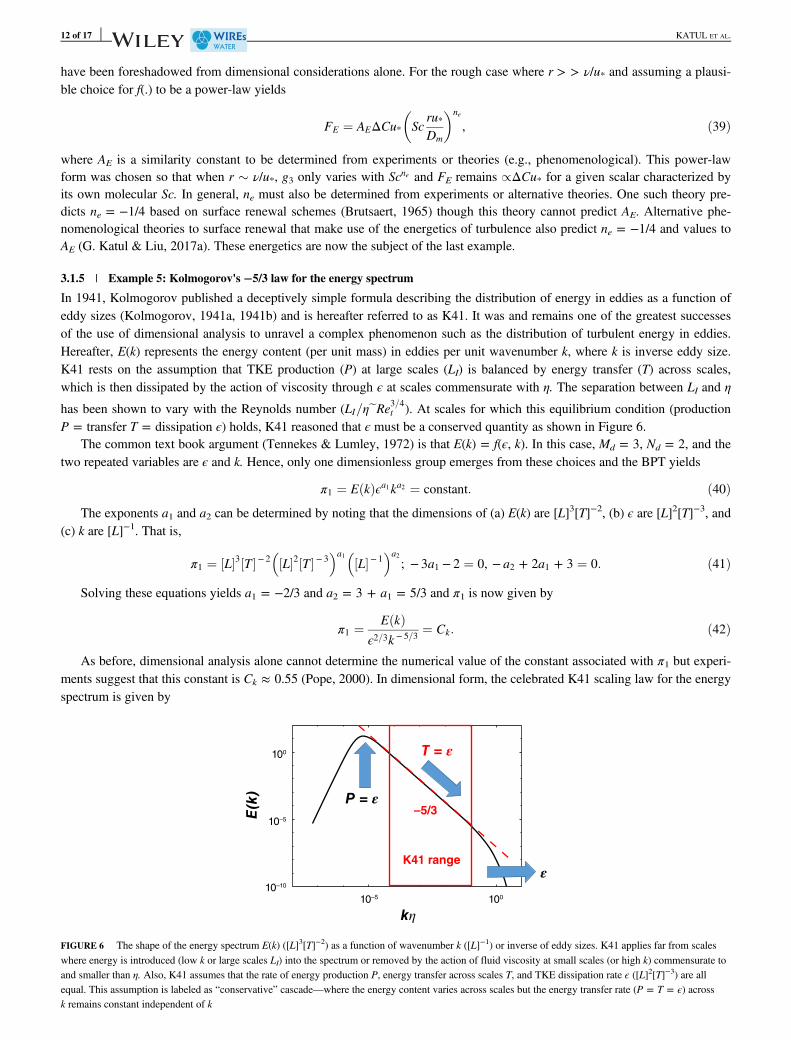
3.1.5 | Example 5: Kolmogorov's −5/3 law for the energy spectrum
In 1941, Kolmogorov published a deceptively simple formula describing the distribution of energy in eddies as a function ofeddy sizes (Kolmogorov, 1941a, 1941b) and is hereafter referred to as K41. It was and remains one of the greatest successesof the use of dimensional analysis to unravel a complex phenomenon such as the distribution of turbulent energy in eddies.Hereafter, E(k) represents the energy content (per unit mass) in eddies per unit wavenumber k, where k is inverse eddy size.K41 rests on the assumption that TKE production (P) at large scales (LI) is balanced by energy transfer (T) across scales,which is then dissipated by the action of viscosity through ϵ at scales commensurate with η. The separation between LI and η
has been shown to vary with the Reynolds number (LI=ηeRe3=4t ). At scales for which this equilibrium condition (productionP = transfer T = dissipation ϵ) holds, K41 reasoned that ϵ must be a conserved quantity as shown in Figure 6.
The common text book argument (Tennekes & Lumley, 1972) is that E(k) = f(ϵ, k). In this case, Md = 3, Nd = 2, and thetwo repeated variables are ϵ and k. Hence, only one dimensionless group emerges from these choices and the BPT yields
π1 ¼ E kð Þϵa1ka2 ¼ constant: ð40ÞThe exponents a1 and a2 can be determined by noting that the dimensions of (a) E(k) are [L]3[T]−2, (b) ϵ are [L]2[T]−3, and
(c) k are [L]−1. That is,
π1 ¼ L½ �3 T½ �− 2 L½ �2 T½ �− 3� �a1
L½ �− 1� �a2
; − 3a1 − 2 ¼ 0, − a2 + 2a1 + 3 ¼ 0: ð41Þ
Solving these equations yields a1 = −2/3 and a2 = 3 + a1 = 5/3 and π1 is now given by
π1 ¼ E kð Þϵ2=3k − 5=3
¼ Ck: ð42Þ
As before, dimensional analysis alone cannot determine the numerical value of the constant associated with π1 but experi-ments suggest that this constant is Ck ≈ 0.55 (Pope, 2000). In dimensional form, the celebrated K41 scaling law for the energyspectrum is given by
kη
P = ε
100
10–5
10–10
10–5 100
ε
T = ε
–5/3
K41 range
E(k
)
FIGURE 6 The shape of the energy spectrum E(k) ([L]3[T]−2) as a function of wavenumber k ([L]−1) or inverse of eddy sizes. K41 applies far from scaleswhere energy is introduced (low k or large scales LI) into the spectrum or removed by the action of fluid viscosity at small scales (or high k) commensurate toand smaller than η. Also, K41 assumes that the rate of energy production P, energy transfer across scales T, and TKE dissipation rate ϵ ([L]2[T]−3) are allequal. This assumption is labeled as “conservative” cascade—where the energy content varies across scales but the energy transfer rate (P = T = ϵ) acrossk remains constant independent of k
12 of 17 KATUL ET AL.
E kð Þ ¼ Ckϵ2=3k − 5=3: ð43Þ
It has been demonstrated that the k−5/3 scaling is associated with eddy sizes contributing to vortex stretching, one of thedefining syndromes of turbulence. For this reason, occurrences of the k−5/3 scaling in experiments have been associated withthe presence of three-dimensional fully developed turbulence at high Re.
To bring this last point into focus, the k−5/3 in K41 does not reflect any boundary conditions or fluid properties. To do sorequires the use of BPT with the additional parameters of domain size Ld and ν. Using a similar approach to the prior exam-ples, E(k) = f(ϵ, k, ν, Ld). Hence, Md = 5, Nd = 2, and upon selecting the repeated variables as in K41 (i.e., ϵ and k), the BPTresults in
π1 ¼ E kð Þϵ2=3k − 5=3
; π2 ¼ νϵa3ka4 ; π3 ¼ Ldϵa5ka6 : ð44Þ
Solving for a3..a6 yields the following: a3 = −1/3, a4 = 4/3, a5 = 0, and a6 = 1 and
π2 ¼ νϵ− 1=3k4=3; π3 ¼ kLd: ð45ÞThe π2 already foreshadows the emergence of the Kolmogorov microscale given as η = (ν3/ϵ)1/4 and can be conveniently
expressed as π2 = (kη)4/3. Hence,
E kð Þ ¼ ϵ2=3k − 5=3f kLd, kηð Þ4=3� �
: ð46Þ
If η and Ld are sufficiently separated scalewise (i.e., η/Ld ! 0), then the function f(.) can be decomposed into the productof two functions correcting K41 scaling at large (kLd � 1) and small (kη � 1) scales. That is,
E kð Þ ¼ ϵ2=3k − 5=3g1 kLdð Þg2 kηð Þ4=3� �
: ð47Þ
Again, BPT cannot predict g1(.) and g2(.). However, g1 must encode the effects of boundary conditions on the shape of thespectrum at large scales, whereas g2 may be more universal across various turbulent flows. This analysis also illustrates whyK41 scaling can only hold for kη < < 1 and kLd > > 1 to ensure g1 and g2 attain constant values.
4 | FURTHER READING
Despite the successes of dimensional analysis in arriving at these empirical formulae, especially those describing the bulk(or macroscopic) flow and transport properties (Examples 1–4), what is evidently missing is the connection between them andthe most prominent features of the flows they describe, namely, the turbulent energetics (or fluctuations) and eddies discussedin Example 5. Establishing the connection through phenomenological theories has been drawing significant research attentionover the past 15 years, which is briefly discussed here. This topic is selected as further reading because it offers new tactics toinfer f(.) that are difficult to achieve via dimensional considerations alone. In certain instances, they offer connections betweencertain constants such as κ and Co thereby providing additional constraints on the problem.
Phenomenological theories built on spectral links, cospectral budget models, and/or structure functions attempt to infer f(.)from the universal character of E(k) in Example 5. A seminal paper by Gioia and Bombardelli (2002) introduced a simplifiedversion of the spectral link to arrive at Manning's formula and the Strickler's scaling (Example 1). Applications of this link tocomplex situations such as flows within emergent and submerged canopies followed with acceptable agreement betweenmodel calculations and measurements (Huthoff, Augustijn, & Hulscher, 2007; Konings, Katul, & Thompson, 2012). Thisapproach was later expanded by relating the energetics of turbulent eddies to the Darcy–Weisbach friction factor fdw (Brown,2002, 2003) thereby explaining, for the first time, the shape of so-called Nikuradse curves (Gioia & Chakraborty, 2006) andMoody charts (Moody, 1944). The linkage between fdw and E(k) may be summarized as:
f dw /ffiffiffiffiffiffiffiffiffiffiffiffiffiffiffiffiffiffiffiffiffið∞
1=lE kð Þdk
s, ð48Þ
and was shown to be consistent with numerical solutions of detailed spectral budgets (Calzetta, 2009), where l = r + aη is acharacteristic scale that includes the surface roughness size r and the Kolmogorov microscale η as before. Equation 48 wasverified using two-dimensional soap film experiments, where E(k) was manipulated so as to scale as k−5/3 or k−3 depending onwhether the inverse energy cascade or forward enstrophy (or integral of vorticity) cascade applies (Guttenberg & Goldenfeld,2009; Kellay et al., 2012; Tran et al., 2010). Another intriguing application of the relation between fdw and E(k) was the correct
KATUL ET AL. 13 of 17
inference of the intermittency exponent (Goldenfeld, 2006; Mehrafarin & Pourtolami, 2008) postulated by Kolmogorov'srefinements to the inertial subrange scaling (Kolmogorov, 1962). To some degree, Equation 48 may be viewed as analogousto a fluctuation (i.e., related to E(k))—dissipation (i.e., related to fdw) phenomenological theory (Kubo, 1966) for turbulence(Goldenfeld & Shih, 2017). The spectral link was also used to highlight how fdw may be enhanced above gravel beds at highReynolds number due to eddy penetration into the porous medium and the resulting faster-than Darcy velocity within thegravel bed itself (Manes, Ridolfi, & Katul, 2012).
In another landmark study, Gioia and coworkers formalized their earlier approach to explain the entire shape of u(z) abovea smooth surface covered in Example 2 starting from an assumed shape of the spectrum of turbulent eddies (Gioia, Gutten-berg, Goldenfeld, & Chakraborty, 2010). Their energy spectrum featured the well-established K41 scaling for inertial sub-range eddies modified to include the effects of TKE generation at larger scales and viscous cutoff at smaller scales (seeEquation 47) as shown in Figure 6. This approach was labeled the “spectral link” because it provides a link between the shapeof the turbulent energy spectrum (i.e., fluctuations) to well-known features in the mean velocity profile (Gioia et al., 2010).
The spectral link was then employed to stratified atmospheric surface layer flows with the goal of deriving the so-calledstability correction function to the mean velocity profile (see Example 3). Two modifications were necessary to implement theoriginal spectral link to atmospheric flows: the inclusion of the effects of thermal stratification on the TKE mean dissipationrate and the eddy-size anisotropy (G. Katul, Konings, & Porporato, 2011). The resulting outcome provided a novel explana-tion for the power-law scaling exponents and coefficients in the stability correction function for momentum transfer. Thus,extensions of the spectral link to stratified atmospheric flows yielded fruitful connections between two separate theories devel-oped by the Russian school of fluid mechanics: Kolmogorov's theory for inertial subrange eddies and Monin–Obukhov simi-larity theory requiring data-derived stability correction functions. It also explained the origin of the so-called OKEYPSequation (after Obukhov–Kazansky–Ellison–Yamamoto–Panofsky–Sellers) describing the stability correction function fromnear convective to mildly stable atmospheric flow (Foken, 2006). The stability correction functions have also been the subjectof an “up-graded” dimensional analysis known as directional-dimensional analysis (Kader & Yaglom, 1990). Here, distinctvelocities are used to normalize horizontal and vertical flow variables instead of only u* offering a more plausible scaling tothe intermediate region between neutral (no heating) and free convective (no shear) conditions.
Refinements were undertaken so as to relax some restrictions on the formulation of eddy-size anisotropy and to extend theaforementioned arguments to mean scalar quantities (G. Katul, Li, Chamecki, & Bou-Zeid, 2013; Li, Katul, & Bou-Zeid,2012; Li, Salesky, & Banerjee, 2016; Salesky, Katul, & Chamecki, 2013). In the process of extending the spectral link to strat-ified turbulent flows, a number of limitations became apparent. The primary one is the oversimplified representation of the tur-bulent shear stress and associated momentum transfer (G. G. Katul, Porporato, et al., 2013), which is assumed to bedominated by a single scale of eddy motion motivated by the so-called attached eddy hypothesis (Townsend, 1976). Thecospectral budget model was then developed to rectify this limitation, allowing for a new representation of the multiscalenature of turbulent transfer. The cospectral budget model recovers and refines the results obtained previously by the spectrallink such as the mean velocity profile above a smooth surface (G. Katul & Manes, 2014; McColl, Katul, Gentine, & Ente-khabi, 2016) and enables extensions to more complex situations as well as to scalar transport (G. Katul, Porporato, Shah, &Bou-Zeid, 2014; Li, Katul, & Bou-Zeid, 2015; Li, Katul, & Zilitinkevich, 2015; G. Katul, Li, Liu, & Assouline, 2016; Liet al., 2016; Li & Katul, 2017; McColl, van Heerwaarden, Katul, Gentine, & Entekhabi, 2017). It also offered a new perspec-tive on the debate about the shape of the mean velocity profile (power-law versus log-law) as discussed elsewhere(G. G. Katul, Porporato, et al., 2013). This work showed that intermittency corrections to the spectrum of turbulence can lead,under some conditions, to power-law solutions for u(z) even at infinite Re.
Phenomenological theories based on structure functions also explain the scaling laws in the evaporation from rough sur-face (see Example 4) when the gas transfer velocity linking FE to ΔC is assumed to follow the K41 scaling subject to the vis-cous corrections derived from the von-Karman–Howarth Equation (G. Katul, Manes, Porporato, Bou-Zeid, & Chamecki,2015), which is equivalent to assuming that eddies responsible for water vapor transfer at the air–surface interface scales withthe Kolmogorov microscale. Such arguments successfully recover the “−1/4” scaling in Equation 39, which was derived inprevious studies based on surface renewal theory (Brutsaert, 1965). The results suggest that the ‘−1/4’ scaling law is an out-come of the Kolmogorov microscale and the associated time scale, while the viscous corrections only alter the scaling of FE
with respect to Sc but not u* (G. Katul & Liu, 2017b). Revisions to surface renewal theories that account for large eddies havebeen proposed and reviewed elsewhere (G. Katul, Mammarella, Grönholm, & Vesala, 2018). These theories confirm that thesimilarity constant AE in Equation 39 vary as power-law with a Reynolds number, a finding that has been confirmed by DNSand several laboratory studies (G. Katul et al., 2018).
Another interfacial phenomenon receiving renewed interest from phenomenological theories is fluvial hydraulics (Ali &Dey, 2018). The spectral link was recently used to explain a number of scaling laws reported experimentally regarding theincipient motion of sediment particles (Ali & Dey, 2017). It was shown that the densimetric Froude number, which describes
14 of 17 KATUL ET AL.
a dimensionless critical bulk velocity to initiate particle movement, can be linked to the submergence depth (r/h) via threescaling laws whose exponents are linked to E(k). These links enlightened how the energetics of turbulence across various r/halters the incipient motion of sediments.
5 | CONCLUSION
To conclude, recent advances in computational and experimental fluid mechanics have allowed for a greater understanding ofmany types of turbulent flows, which are universally considered as one of the main drivers of hydrological and hydraulic pro-cesses; despite these advances, hydraulics and hydrology practice has not effectively profited from them. Undoubtedly, theslow infusion of new knowledge into practice is related to the fact that mathematical treatment of turbulence as well as theunderstanding of its underpinning physics can be daunting and often accessible only to specialists. Fortunately, to amelioratethe situation, dimensional analysis has historically represented a powerful tool that, while bypassing the intricacies of turbu-lence theory, allows for the derivation of many formulae that are still routinely used in many problems of practical interestdealing with highly turbulent flows. This justifies the choice of the authors of writing a primer on turbulence specificallyfocused on dimensional analysis. However, a word of caution is in order here. The title of this primer should not fool thereader as dimensional analysis can be indeed a powerful tool but it should be considered by no means as the panacea for turbu-lent flows. After reading the present paper, the reader is now probably aware that significant results from dimensional analysiscan be reached when the number of nondimensional groups governing the phenomenon is little and allows for the applicationof similarity principles. Moreover, the selection of these groups and governing variables requires deep understanding and intu-ition about the turbulent transport phenomenon. On the contrary, many problems in hydrology and hydraulics are governed bya large number of nondimensional groups, which makes it difficult to apply such principles and even to empirically explorefunctional relations among groups as these are heavily interlinked (Manes & Brocchini, 2015). As discussed in the previoussection, another shortcoming of dimensional analysis is that it represents, by definition, a mathematical tool that is almostcompletely disconnected from the features of the flows it describes and, therefore, it is often bound to offer incomplete solu-tions that can be susceptible to scale issues. Lately, phenomenological theories based on the so-called spectral and cospectralbudget approaches have offered an alternative to dimensional analysis to identify and recover laws of practical interest. Thetheoretical background to understand and apply such phenomenological approaches is clearly heavier when compared todimensional analysis. Nonetheless they represent, to the authors’ opinion, an exciting tool that may even accelerate the bridg-ing between theory and practice in ways that still await discovery. For this reason, they are proposed as further reading to thereader seeking description of hydraulics and hydrology that goes beyond empirical laws.
ACKNOWLEDGMENTS
The authors thank A. Mrad, Y. Liu, and E. Zorzetto for helpful comments and suggestions. G.K. acknowledges support fromthe U.S. National Science Foundation (NSF-EAR-1344703, NSF-AGS-1644382, and NSF-IOS-1754893). D.L. acknowledgessupport from the U.S. Army Research Office (W911NF-18-1-0360). C.M. acknowledges support from “Compagnia di SanPaolo” (project: “Attrarre Docenti di Qualità tramite Starting Grant”).
CONFLICT OF INTEREST
The authors have declared no conflicts of interest for this article.
RELATED WIREs ARTICLES
The hydraulic description of vegetated river channels: the weaknesses of existing formulations and emerging alternativesLife in turbulent flows: interactions between hydrodynamics and aquatic organisms in rivers
REFERENCES
Ali, S. Z., & Dey, S. (2017). Origin of the scaling laws of sediment transport. Proceedings of the Royal Society A, 473(2197), 20160785.Ali, S. Z., & Dey, S. (2018). Impact of phenomenological theory of turbulence on pragmatic approach to fluvial hydraulics. Physics of Fluids, 30(4), 045105.Barenblatt, G. (1996). Scaling self-similarity, and intermediate asymptotics. Cambridge, England: Cambridge University Press.Barenblatt, G., & Chorin, A. J. (1998). New perspectives in turbulence: Scaling laws, asymptotics, and intermittency. SIAM Review, 40(2), 265–291.Bonetti, S., Manoli, G., Manes, C., Porporato, A., & Katul, G. (2017). Manning's formula and Strickler's scaling explained by a co-spectral budget model. Journal of
Fluid Mechanics, 812, 1189–1212.Brown, G. (2002). Henry Darcy and the making of a law. Water Resources Research, 38(7), 1–12.
Brown, G. (2003). The history of the Darcy-Weisbach equation for pipe flow resistance. In J. R. Rogers & A. J. Fredrich (Eds.), Proceedings from the ASCE Civil Engi-neering Conference and Exposition, 2002, November 3–7, 2002, Washington, D.C., United States (pp. 34–43). https://doi.org/10.1061/9780784406502.fm
Brutsaert, W. (1965). A model for evaporation as a molecular diffusion process into a turbulent atmosphere. Journal of Geophysical Research, 70(20), 5017–5024.Brutsaert, W. (1982). Evaporation into the atmosphere: Theory, history, and applications. Dordrecht, Holland: Reidel Co.Brutsaert, W. (2005). Hydrology: An Introduction. Cambridge, England: Cambridge University Press.Buckingham, E. (1914). On physically similar systems: Illustrations of the use of dimensional equations. Physical Review, 4(4), 345–376.Businger, J., & Yaglom, A. (1971). Introduction to Obukhov's paper on ‘turbulence in an atmosphere with a non-uniform temperature’. Boundary-Layer Meteorology,
2(1), 3–6.Calzetta, E. (2009). Friction factor for turbulent flow in rough pipes from Heisenberg's closure hypothesis. Physical Review E, 79(5), 056311.Chézy, A. (1775). Memoire sur la vitesse de l'eau conduit dans une rigole donne. Dossier, 847, 363–368.Chow, V. T. (Ed.). (1959). Open Channel hydraulics. New York, NY: McGraw-Hill.D'arcy, W. T. (1915). Galileo and the principle of similitude. Nature, 95(2381), 426.Drazin, P. G., & Reid, W. H. (2004). Hydrodynamic stability. Cambridge, England: Cambridge University Press.Foken, T. (2006). 50 years of the Monin–Obukhov similarity theory. Boundary-Layer Meteorology, 119(3), 431–447.French, R. H. (1985). Open-channel hydraulics. New York, NY: McGraw-Hill.Frisch, U. (Ed.). (1995). Turbulence. Cambridge, England: Cambridge University Press.Gioia, G., & Bombardelli, F. (2002). Scaling and similarity in rough channel flows. Physical Review Letters, 88, 014501.Gioia, G., & Chakraborty, P. (2006). Turbulent friction in rough pipes and the energy spectrum of the phenomenological theory. Physical Review Letters, 96, 044502.Gioia, G., Guttenberg, N., Goldenfeld, N., & Chakraborty, P. (2010). Spectral theory of the turbulent mean-velocity profile. Physical Review Letters, 105(18), 184501.Gleick, J. (2011). Chaos: Making a new science. London, England: Open Road Media.Goldenfeld, N. (2006). Roughness-induced critical phenomena in a turbulent flow. Physical Review Letters, 96(4), 044503.Goldenfeld, N., & Shih, H. (2017). Turbulence as a problem in non-equilibrium statistical mechanics. Journal of Statistical Physics, 167(3–4), 575–594.Guttenberg, N., & Goldenfeld, N. (2009). Friction factor of two-dimensional rough-boundary turbulent soap film flows. Physical Review E, 79(6), 065306.Huthoff, F., Augustijn, D., & Hulscher, S. (2007). Analytical solution of the depth-averaged flow velocity in case of submerged rigid cylindrical vegetation. Water
Resources Research, 43(6). https://doi.org/10.1029/2006WR005625Kader, B., & Yaglom, A. (1990). Mean fields and fluctuation moments in unstably stratified turbulent boundary layers. Journal of Fluid Mechanics, 212, 637–662.Kaimal, J. C., & Finnigan, J. J. (1994). Atmospheric boundary layer flows: Their structure and measurement. Oxford, England: Oxford University Press.Katul, G., & Chu, C.-R. (1998). A theoretical and experimental investigation of energy-containing scales in the dynamic sublayer of boundary-layer flows. Boundary-
Layer Meteorology, 86(2), 279–312.Katul, G., Hsieh, C.-I., & Sigmon, J. (1997). Energy-inertial scale interactions for velocity and temperature in the unstable atmospheric surface layer. Boundary-Layer
Meteorology, 82(1), 49–80.Katul, G., Konings, A., & Porporato, A. (2011). Mean velocity profile in a sheared and thermally stratified atmospheric boundary layer. Physical Review Letters,
107(26), 268502.Katul, G., Li, D., Chamecki, M., & Bou-Zeid, E. (2013). Mean scalar concentration profile in a sheared and thermally stratified atmospheric surface layer. Physical
Review E, 87(2), 023004.Katul, G., Li, D., Liu, H., & Assouline, S. (2016). Deviations from unity of the ratio of the turbulent Schmidt to Prandtl numbers in stratified atmospheric flows over
water surfaces. Physical Review Fluids, 1(3), 034401.Katul, G., & Liu, H. (2017a). A Kolmogorov-Brutsaert structure function model for evaporation into a turbulent atmosphere. Water Resources Research, 53(5),
3635–3644.Katul, G., & Liu, H. (2017b). Multiple mechanisms generate a universal scaling with dissipation for the air-water gas transfer velocity. Geophysical Research Letters,
44(4), 1892–1898.Katul, G., Mammarella, I., Grönholm, T., & Vesala, T. (2018). A structure function model recovers the many formulations for air-water gas transfer velocity. Water
Resources Research, 54(9), 5905–5920.Katul, G., & Manes, C. (2014). Cospectral budget of turbulence explains the bulk properties of smooth pipe flow. Physical Review E, 90, 063008.Katul, G., Manes, C., Porporato, A., Bou-Zeid, E., & Chamecki, M. (2015). Bottlenecks in turbulent kinetic energy spectra predicted from structure function inflections
using the von Kármán-Howarth equation. Physical Review E, 92(3), 033009.Katul, G., Porporato, A., Shah, S., & Bou-Zeid, E. (2014). Two phenomenological constants explain similarity laws in stably stratified turbulence. Physical Review E,
89(1), 023007.Katul, G., Wiberg, P., Albertson, J. D., & Hornberger, G. (2002). A mixing layer theory for flow resistance in shallow streams. Water Resources Research, 38, 1–8.Katul, G. G., Porporato, A., Manes, C., & Meneveau, C. (2013). Co-spectrum and mean velocity in turbulent boundary layers. Physics of Fluids, 25(9), 091702.Kellay, H., Tran, T., Goldburg, W., Goldenfeld, N., Gioia, G., & Chakraborty, P. (2012). Testing a missing spectral link in turbulence. Physical Review Letters,
109(25), 254502.Keulegan, G. H. (1938). Laws of turbulent flow in open channels (Vol. 21, pp. 707–741). Gaithersburg, MD: National Bureau of Standards US.Kolmogorov, A. (1941a). Dissipation of energy under locally isotropic turbulence. Doklady Akademiia Nauk SSSR, 32, 16–18.Kolmogorov, A. (1941b). The local structure of turbulence in incompressible viscous fluid for very large Reynolds numbers. Doklady Akademiia Nauk SSSR, 30,
299–303.Kolmogorov, A. (1962). A refinement of previous hypotheses concerning the local structure of turbulence in a viscous incompressible fluid at high Reynolds number.
Journal of Fluid Mechanics, 13(1), 82–85.Konings, A., Katul, G., & Thompson, S. (2012). A phenomenological model for the flow resistance over submerged vegetation. Water Resources Research, 48(2).
https://doi.org/10.1029/2011WR011000Kubo, R. (1966). The fluctuation-dissipation theorem. Reports on Progress in Physics, 29(1), 255–284.Lemons, D. S. (2018). Dimensional analysis for curious undergraduates: A student's guide to dimensional analysis. Cambridge, MA: Cambridge University Press.Li, D., Katul, G., & Bou-Zeid, E. (2012). Mean velocity and temperature profiles in a sheared diabatic turbulent boundary layer. Physics of Fluids, 24(10), 105105.Li, D., Katul, G., & Bou-Zeid, E. (2015). Turbulent energy spectra and cospectra of momentum and heat fluxes in the stable atmospheric surface layer. Boundary-Layer
Meteorology, 157(1), 1–21.Li, D., & Katul, G. G. (2017). On the linkage between the k−5/3 spectral and k−7/3 cospectral scaling in high-Reynolds number turbulent boundary layers. Physics of
Fluids, 29(6), 065108.Li, D., Katul, G. G., & Zilitinkevich, S. S. (2015). Revisiting the turbulent Prandtl number in an idealized atmospheric surface layer. Journal of the Atmospheric Sci-
ences, 72(6), 2394–2410.Li, D., Salesky, S., & Banerjee, T. (2016). Connections between the Ozmidov scale and mean velocity profile in stably stratified atmospheric surface layers. Journal of
Lorenz, E. N. (1963). Deterministic nonperiodic flow. Journal of the Atmospheric Sciences, 20(2), 130–141.Manes, C., & Brocchini, M. (2015). Local scour around structures and the phenomenology of turbulence. Journal of Fluid Mechanics, 779, 309–324.Manes, C., Ridolfi, L., & Katul, G. (2012). A phenomenological model to describe turbulent friction in permeable-wall flows. Geophysical Research Letters, 39(14).
https://doi.org/10.1029/2012GL052369Manning, R. (1891). On the flow of water in open channels and pipes. Transactions of the Institution of Civil Engineers of Ireland, 20, 161–207.McColl, K. A., Katul, G. G., Gentine, P., & Entekhabi, D. (2016). Mean-velocity profile of smooth channel flow explained by a cospectral budget model with wall-
blockage. Physics of Fluids, 28(3), 035107.McColl, K. A., van Heerwaarden, C. C., Katul, G. G., Gentine, P., & Entekhabi, D. (2017). Role of large eddies in the breakdown of the Reynolds analogy in an ideal-
ized mildly unstable atmospheric surface layer. Quarterly Journal of the Royal Meteorological Society, 143(706), 2182–2197.Mehrafarin, M., & Pourtolami, N. (2008). Intermittency and rough-pipe turbulence. Physical Review E, 77(5), 055304.Merlivat, L. (1978). The dependence of bulk evaporation coefficients on air-water interfacial conditions as determined by the isotopic method. Journal of Geophysical
Research: Oceans, 83(C6), 2977–2980.Monin, A., & Obukhov, A. (1954). Basic laws of turbulent mixing in the surface layer of the atmosphere. Trudy Geofiz, Instituta Akademii Nauk, SSSR, 24(151),
163–187.Moody, L. (1944). Friction factors for pipe flow. Transactions of the ASME, 66, 671–684.Pomeau, Y. (2016). The long and winding road. Nature Physics, 12(3), 198–199.Pope, S. B. (Ed.). (2000). Turbulent flows. Cambridge, England: Cambridge Univeristy Press.Rayleigh, L. (1915). The principle of similitude. Nature, 95, 66–68.Richardson, L. F. (1922). Weather prediction by numerical methods. Cambridge, England: Cambridge University Press.Salesky, S., Katul, G., & Chamecki, M. (2013). Buoyancy effects on the integral lengthscales and mean velocity profile in atmospheric surface layer flows. Physics of
Fluids, 25(10), 105101.Succi, S. (2001). The lattice Boltzmann equation: For fluid dynamics and beyond. Oxford, England: Oxford University Press.Tennekes, H., & Lumley, J. L. (1972). A first course in turbulence. Cambridge, MA: MIT press.Townsend, A. (1976). The structure of turbulent shear flow. Cambridge, MA: Cambridge University Press.Tran, T., Chakraborty, P., Guttenberg, N., Prescott, A., Kellay, H., Goldburg, W., … Gioia, G. (2010). Macroscopic effects of the spectral structure in turbulent flows.
Nature Physics, 6(6), 438–441.Willcocks, W., & Holt, R. (Eds.). (1899). Elementary hydraulics. Cairo, Egypt: National Printing Office.
How to cite this article: Katul G, Li D, Manes C. A primer on turbulence in hydrology and hydraulics: The power ofdimensional analysis. WIREs Water. 2019;e1336. https://doi.org/10.1002/wat2.1336