A Process Integration Primer - IETS

SINTEF Energy Research IEA Primer on Process Integration

Page 1 of 90

International Energy Agency

Implementing Agreement on Process IntegrationAnnex I (Survey and Strategy)

Supported byCanada, Denmark, Finland, Portugal, Sweden, Switzerland and UK

AProcess

Integration

PRIMERby

Truls GundersenOperating Agent

SINTEF Energy ResearchDept. of Thermal Energy and Hydro Power

Trondheim, Norway

© SINTEF Energy Research3rd and Final version, 9 April 2002

Copying is free within the Participating countriesof the IEA Implementing Agreement on Process Integration


Page 2 of 90


Page 3 of 90

LIST OF CONTENTS

Summary 5

1. Background 5

2. Introduction 6

2.1 Definition of Process Integration 6

2.2 Current Status of Process Integration 7

2.3 From History to the Future 8

2.4 Process Integration and the “Pinch” Concept 8

2.5 Performance Targets before Design 9

2.6 Schools of Methods in Process Integration 9

3. Process Integration Application Areas 10

3.1 Classification of Industrial Tasks 10

3.2 Some Useful Representations 11

4. Sequence of Presentation 12

5. Basic Concepts for Heat Recovery inNew Design of Continuos Processes 13

5.1 Data Extraction (Phase 1) 13

5.2 Performance Targets (Phase 2) 15

5.3 Network Design (Phase 3) 26

5.4 Network Optimization (Phase 4) 29

6. Basic Concepts for Heat Recovery inRetrofit Design of Continuous Processes 34

6.1 Some Useful Representations 34

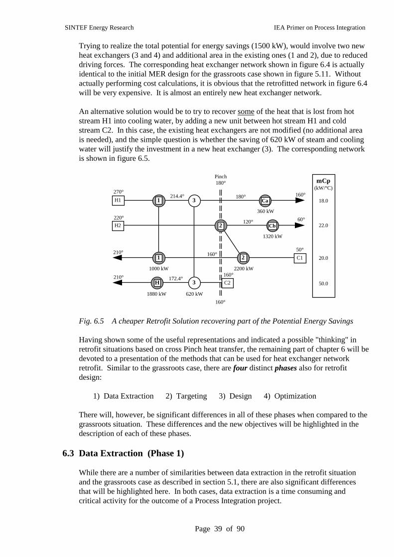
6.2 A Preliminary Retrofit Discussion 38


6.4 Retrofit Targets (Phase 2) 40

6.5 Retrofit Design (Phase 3) 44



Page 4 of 90

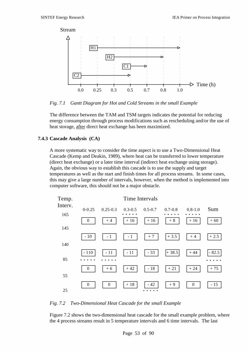
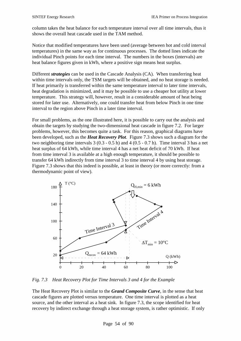
7. Basic Concepts for Heat Recoveryin Batch Processes 49

7.1 Introduction 49

7.2 Heat Recovery and Design Phases 49


7.4 Energy Targeting (Phase 2) 51

7.5 Network Design (Phase 3) 57


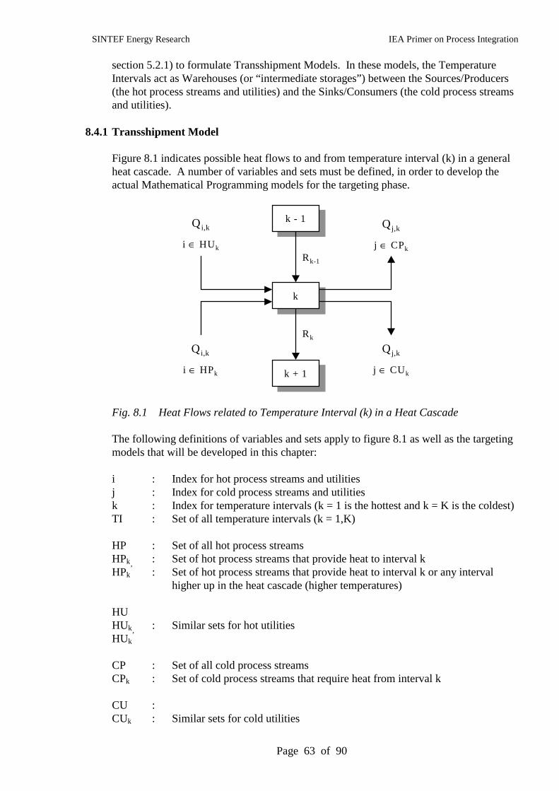
8. Basic Concepts for Using MathematicalProgramming in Process Integration 60

8.1 Motivation 60

8.2 A Brief History 61

8.3 Classes of Mathematical Programming Models 62

8.4 Rigorous Targets for Heat Integration 62

8.5 Network Design using Mathematical Programming 73

8.6 Summary 77

9. Advances in Process Integration 78

9.1 Structuring the Material 78

9.2 Reactor Systems 78

9.3 Separation Systems 78

9.4 Heat Exchanger Networks 79

9.5 Exergy Considerations in Process Integration 80

9.6 Advanced Methods for Utility Systems 81

9.7 Analogies to the Heat Recovery Pinch 81

9.8 Component Considerations in Systems Technologies 82

References 84

Text Book References 89


Page 5 of 90

SUMMARY

This Primer can be regarded as a stand-alone document intended to convey the most basicaspects of Process Integration methods. It also contains towards the end some detailsabout the more recent and advanced elements of Process Integration methods. Sinceemphasis is on learning, the number of references is kept at a minimum, especially in thecore chapters of this Primer.

The Primer is one of the products from the Process Integration Implementing Agreementwithin the International Energy Agency (IEA). The other main products from Annex I(Survey and Strategy) of this IEA Agreement are:

• “IEA Implementing Agreement on Process Integration: Annex I End-User Survey”,T.J. Pears, EA Technology, Capenhurst, UK, November 1997.

• “A Worldwide Catalogue on Process Integration”, T. Gundersen, Telemark Institute ofTechnology, Porsgrunn, Norway, December 1997.

The Primer contains some general material on Process Integration (chapters 1, 2 and 3) inaddition to the more tutorial chapters (5, 6, 7 and 8), and one chapter (9) on more advancedaspects of Process Integration. In the first part, there is some information about the IEAproject, and the Primer attempts to put Process Integration into a broader perspective.

1. BACKGROUND

The Implementing Agreement on Process Integration within the International EnergyAgency (IEA) was formally started in September 1995, motivated by the recognition thatProcess Integration was not used to its full potential in industry, with significantdifferences across geographical regions and industrial branches.

This Primer is based on the idea that there was a need for a document similar to the PinchTechnology Primer that was prepared by Linnhoff March and published by EPRI about tenyears ago (1991). Since Process Integration has been expanded considerably and goes farbeyond basic Pinch Technology, there is a need for a new Primer that describes the morerecent developments. For completeness reasons, however, it was decided to include alsothe more basic and established parts of Process Integration methods.

Emphasis in the presentation of the material will be on what can be done, rather than howit is done. The Primer is written for practitioners in the process industries, and those thatare interested in more details will have to consult some of the literature that is referencedhere, both the journal papers and the growing number of text books available.

Finally, this Primer is expected to be one of many ways to disseminate knowledge aboutProcess Integration into operating companies, engineering and contracting companies,consultants and even software vendors. Information about the IEA Agreement on ProcessIntegration can be found on the Web site http://www.tev.ntnu.no/iea/pi/.


Page 6 of 90

2. INTRODUCTION

The structure of the Primer has been designed to hopefully allow practitioners in industryto get a smooth introduction to Process Integration methods, with its powerful concepts,representations and graphical diagrams. Gradually, the Primer will provide more detailedinformation about application areas and relevant methods. For details about ProcessIntegration Technologies, the reader will have to refer to some of the recommendedliterature given as references in this Primer. A number of good text books and overviewarticles also exist that will be referred to.

2.1 Definition of Process Integration

Process Integration is a fairly new term that emerged in the 80's and has been extensivelyused in the 90's to describe certain Systems oriented activities related primarily to ProcessDesign. It has incorrectly been interpreted as Heat Integration by a lot of people, probablycaused by the fact that Heat Recovery studies inspired by the Pinch Concept initiated thefield and are still core elements of Process Integration. It appears to be a rather dynamicfield, with new methods and application areas emerging constantly. The definition used inthis context is the one used by the IEA since 1993:

"Systematic and General Methods for Designing Integrated Production Systems,ranging from Individual Processes to Total Sites, with special emphasis on theEfficient Use of Energy and reducing Environmental Effects".

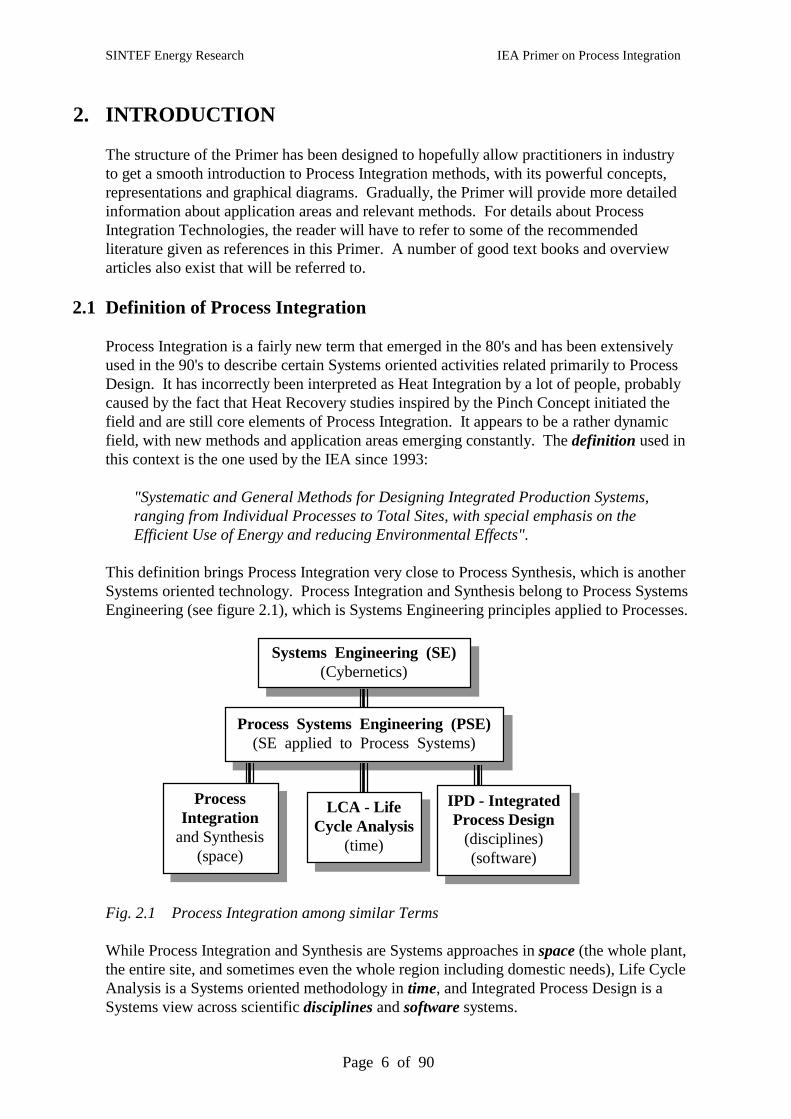
This definition brings Process Integration very close to Process Synthesis, which is anotherSystems oriented technology. Process Integration and Synthesis belong to Process SystemsEngineering (see figure 2.1), which is Systems Engineering principles applied to Processes.

Systems Engineering (SE)(Cybernetics)

Process Systems Engineering (PSE)(SE applied to Process Systems)

IPD - IntegratedProcess Design

(disciplines)(software)

LCA - LifeCycle Analysis

(time)

ProcessIntegration

and Synthesis(space)

Fig. 2.1 Process Integration among similar Terms

While Process Integration and Synthesis are Systems approaches in space (the whole plant,the entire site, and sometimes even the whole region including domestic needs), Life CycleAnalysis is a Systems oriented methodology in time, and Integrated Process Design is aSystems view across scientific disciplines and software systems.


Page 7 of 90

When using the term Process Integration, we both refer to certain industrial tasks and toclasses of methods to address these tasks. In this Primer, we will concentrate on methodsthat have been developed specifically to address these tasks, however, there are also anumber of methods of a more general nature that can be used to a larger or smaller extentto solve Process Integration problems. These methods will also be briefly described.

2.2 Current Status of Process Integration

Process Integration is a strongly growing field of Process Engineering. It is now standardcurriculum for process engineers in both Chemical and Mechanical Engineering at mostuniversities around the world, either as a separate topic or as part of a Process Design orSynthesis course. At UMIST (Manchester, UK) there is a separate Department of ProcessIntegration. Research at UMIST has for 15 years been supported by a large number ofindustrial companies through a Consortium that was established in 1984. As part of theIEA project on Process Integration, we have identified about 35 other universities aroundthe world involved in research in this field.

While Heat Recovery was the initial focus of Process Integration, the scope has beenexpanded considerably during the late 80's and the 90's to cover several aspects of ProcessDesign. A key feature of this expansion has been the use of basic concepts from heatrecovery in other areas through the use of analogies. This has, for example, made itpossible to use heat recovery techniques to study Mass Transfer processes in general andWater Management in particular. Unfortunately, the last attempt to review the entire field(Gundersen and Naess, 1988) is way out of date. The growth of Process Integration duringthe last 10 years has made it almost intractable to produce an updated review.

Appropriate tools, such as user-friendly and reliable software, are keys to industrial use,and there are now around 50 computer programs available to assist the engineer in one ormore areas of Process Integration. This software covers a wide range of problem areas,and the quality of the software is ranging from high standard commercial products beingused routinely in industry, to prototype software from universities that were developedprimarily to assist research. Some of this software may even be available free of charge.

There is an increasing international co-operation on Process Integration. The IEA projecthas already been mentioned, and it is at present supported by seven countries (Canada,Denmark, Finland, Sweden, Switzerland, Portugal and UK). Within the Nordic EnergyResearch Programme, Process Integration has been one of seven activities since 1995. TheEuropean Commission is also funding research in the area of Process Integration.Typically, these projects have a broad international representation.

While the field of Process Integration in the past has been allocated one or two singlesessions on large international meetings, the trend today is to have separate conferencesfocusing specifically on Process Integration. Examples include PRES'98 (Prague), PI'99(Copenhagen), PRES'99 (Budapest), and continuing with PRES'2000 (Prague).

In conclusion, Process Integration has evolved from a Heat Recovery methodology in the80's to become what a number of leading industrial companies in the 90's regarded as aMajor Strategic Design and Planning Technology. With this technology, it is possible tosignificantly reduce the operating cost of existing plants, while new processes often can bedesigned with reductions in both investment cost and operating cost.


Page 8 of 90

2.3 From History to the Future

Process Design has evolved through distinct "generations". Originally (first generation),inventions that were based on experiments in the laboratory by the chemists, were tested inpilot plants before plant construction. The second generation of Process Design was basedon the concept of Unit Operations, which founded Chemical Engineering as a discipline.Unit Operations acted as building blocks for the engineer in the design process. The thirdgeneration considered integration between these units; for example heat recovery betweenrelated process streams to save energy.

A strong trend today (fourth generation) is to move away from Unit Operations and focuson Phenomena. Processes based on the Unit Operations concept tend to have manyprocess units with significant and complex piping arrangements between the units. Byallowing more than one phenomena (reaction, heat transfer, mass transfer, etc.) to takeplace within the same piece of equipment, significant savings have been observed both ininvestment cost and in operating cost (energy and raw materials). Most of the industrialapplications of this idea have been based on trial and error. Research is progressing,however, trying to develop systematic methods in this area to replace trial and error. Nodoubt, this will affect the discipline of Process Integration, since we no longer look atintegration between units only, but also at integration within units.

2.4 Process Integration and the "Pinch" Concept

The single most important concept and the one that originally gave birth to the field ofProcess Integration is the Heat Recovery Pinch, discovered independently by Hohmann(71), Umeda et al. (78-79) and Linnhoff et al. (78-79). It was Linnhoff's group at UMISTin Manchester, however, that developed this concept into an industrial technology in the80's. The concept has later been expanded into new areas by using various analogies.

The most obvious analogy is between heat transfer and mass transfer. In heat transfer, heatis transferred with temperature difference as the driving force. Similarly, in mass transfer,mass (or certain components) is transferred with concentration difference as the drivingforce. The corresponding Mass Pinch, developed by El-Halwagi and Manousiouthakis(89-90), has a number of industrial applications whenever process streams are exchangingmass in a number of mass transfer units, such as absorbers, extractors, etc.

One specific application of the Mass Pinch is in the area of Wastewater Minimization,where optimal use of water and wastewater is achieved through reuse, regeneration andpossibly recycling. The corresponding Water Pinch, developed by Wang and Smith (94),can also be applied for design of Distributed Effluent Treatment processes.

The most recent extension is the Hydrogen Pinch technology, developed by Towler andAlves (96-99). Oil refineries experience these days an increasing need for hydrogen tomeet new product specifications (for example on diesel and gasoline). The HydrogenPinch method is a tool to optimize the hydrogen distribution system and to evaluate thescope for introducing purification units (such as PSA, membranes and cryogenic units).

In summary, the Pinch concept is a Systems tool since it provides critical information on atotal plant or even site level. The concept is also (as shown above) generally applicable inother areas than heat recovery. Actually, whenever an amount (heat or mass) has a quality


Page 9 of 90

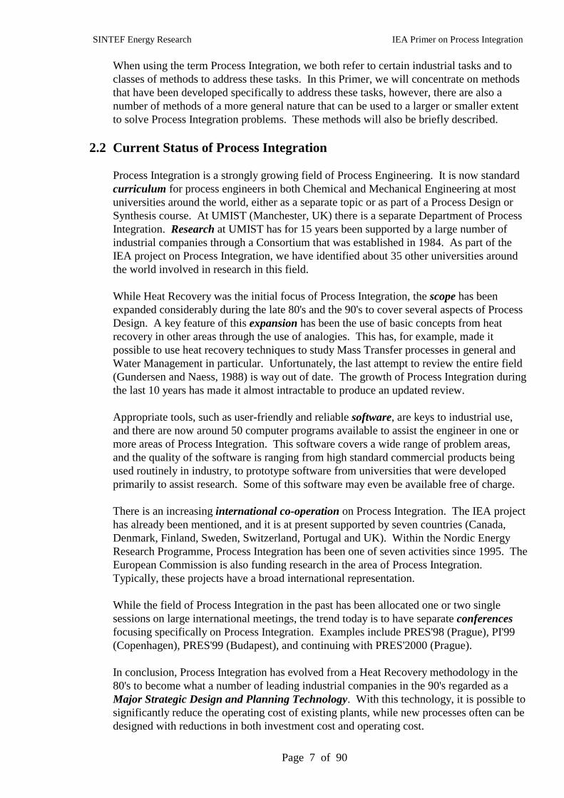
(temperature or concentration), the concept of Composite Curves provides a Systems viewof the problem concerning efficient recovery (or re-use) of resources. The "Pinch" thenshows the location on these curves where there is an accumulated deficit of an amountabove a certain quality. Figure 2.2 shows Composite Curves for a Heat Recovery problem(left) and a Wastewater Minimization application (right).

T

Q

QH,min

QC,min

C

m

LimitingWaterProfile

Water Target

Temperature vs. Enthalpy Concentration vs. Mass Load

Fig. 2.2 The General Concept of Composite Curves applied to Heat and Mass Transfer

2.5 Performance Targets before Design

In the previous section, it was concluded that the Composite Curves represent a conceptthat is general and fundamental in Process Engineering. Another important concept from"early days" Pinch Technology is the idea of establishing objective performance targetsbefore going into the design phase. Examples of such targets in the area of heat recoveryare figures for minimum energy consumption, fewest number of heat transfer equipment,minimum total heat transfer area, and minimum total annual cost. While some of thesetargets are based on thermodynamics (such as energy), others are based on heuristic rules(such as the fewest number of heat exchangers). Finally, some targets are actually onlyestimates of the best performance (such as heat transfer area and total annual cost).

Examples of other targets in Process Integration include minimum wastewater, minimumshaftwork in low temperature processes, minimum emissions, maximum power productionfor total sites, etc. All these and previously mentioned targets have two important features:

1) Any design can be objectively compared with the "best possible".2) The way some targets are calculated also provides guidelines for design.

In his text book on Chemical Process Design, Smith (1995) puts strong emphasis on theidea of establishing Performance Targets prior to Design.

2.6 Schools of Methods in Process Integration

The three major features of Process Integration methods are the use heuristics (insight),about design and economy, the use of thermodynamics and the use of optimizationtechniques. There is significant overlap between the various methods and the trend todayis strongly towards methods using all three features mentioned above. The large number


Page 10 of 90

of structural alternatives in Process Design (and Integration) is significantly reduced by theuse of insight, heuristics and thermodynamics, and it then becomes feasible to address theremaining problem and its multiple economic trade-offs with optimization techniques.

Despite the merging trend mentioned above, it is still valid to say that Pinch Analysis andExergy Analysis are methods with a particular focus on Thermodynamics. HierarchicalAnalysis and Knowledge Based Systems are rule-based approaches with the ability tohandle qualitative (or fuzzy) knowledge. Finally, Optimization techniques can be dividedinto deterministic (Mathematical Programming) and non-deterministic methods (stochasticsearch methods such as Simulated Annealing and Genetic Algorithms).

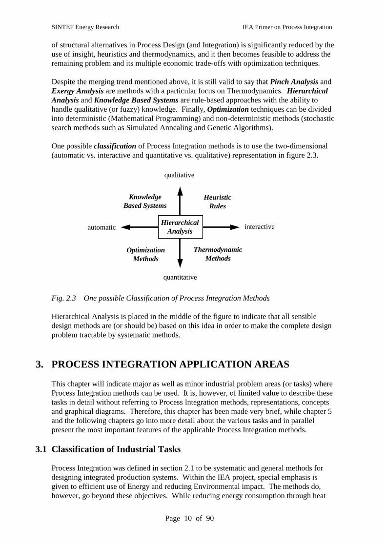
One possible classification of Process Integration methods is to use the two-dimensional(automatic vs. interactive and quantitative vs. qualitative) representation in figure 2.3.

quantitative

qualitative

automatic interactive

OptimizationMethods

ThermodynamicMethods

KnowledgeBased Systems

HeuristicRules

HierarchicalAnalysis

Fig. 2.3 One possible Classification of Process Integration Methods

Hierarchical Analysis is placed in the middle of the figure to indicate that all sensibledesign methods are (or should be) based on this idea in order to make the complete designproblem tractable by systematic methods.

3. PROCESS INTEGRATION APPLICATION AREAS

This chapter will indicate major as well as minor industrial problem areas (or tasks) whereProcess Integration methods can be used. It is, however, of limited value to describe thesetasks in detail without referring to Process Integration methods, representations, conceptsand graphical diagrams. Therefore, this chapter has been made very brief, while chapter 5and the following chapters go into more detail about the various tasks and in parallelpresent the most important features of the applicable Process Integration methods.

3.1 Classification of Industrial Tasks

Process Integration was defined in section 2.1 to be systematic and general methods fordesigning integrated production systems. Within the IEA project, special emphasis isgiven to efficient use of Energy and reducing Environmental impact. The methods do,however, go beyond these objectives. While reducing energy consumption through heat


Page 11 of 90

recovery normally increases investment cost, Process Integration methods also enableindustries to reduce equipment cost for a specified level of energy usage.

Process Integration also affects raw material utilization, since it has been shown thatimproved heat recovery will allow increased recycling in the process. In this way, rawmaterial is used to maximize yield of the desired product and not being lost in lessvaluable outlet streams. Also, increased recycling may allow reduced reactor conversion(per pass), which may improve reactor selectivity and reduce byproduct formation.

The following list of keywords and activities indicate typical application areas of ProcessIntegration for a large number of industrial branches:

• Planning, Design and Operation of Processes and Utility Systems • Short Term (Scheduling) and Long Term Planning (including Strategic Planning) • New Designs and various Retrofit Projects • Improving Efficiency (Energy and Raw Material) and Productivity (Debottlenecking) • Continuous, Semi-Continuous and Batch Processes • All aspects of Processes, such as Reactors, Separators and Heat Exchanger Networks • Integration between the Process and the Utility System • Integration between Processes w.r.t. Material Streams and Energy Streams • Integration between Industrial Sites, Power Stations and District Heating/Cooling • Operability Issues (Flexibility, Controllability and Switchability) • Waste and Wastewater Minimization • Various aspects of Emissions Reduction

3.2 Some Useful Representations

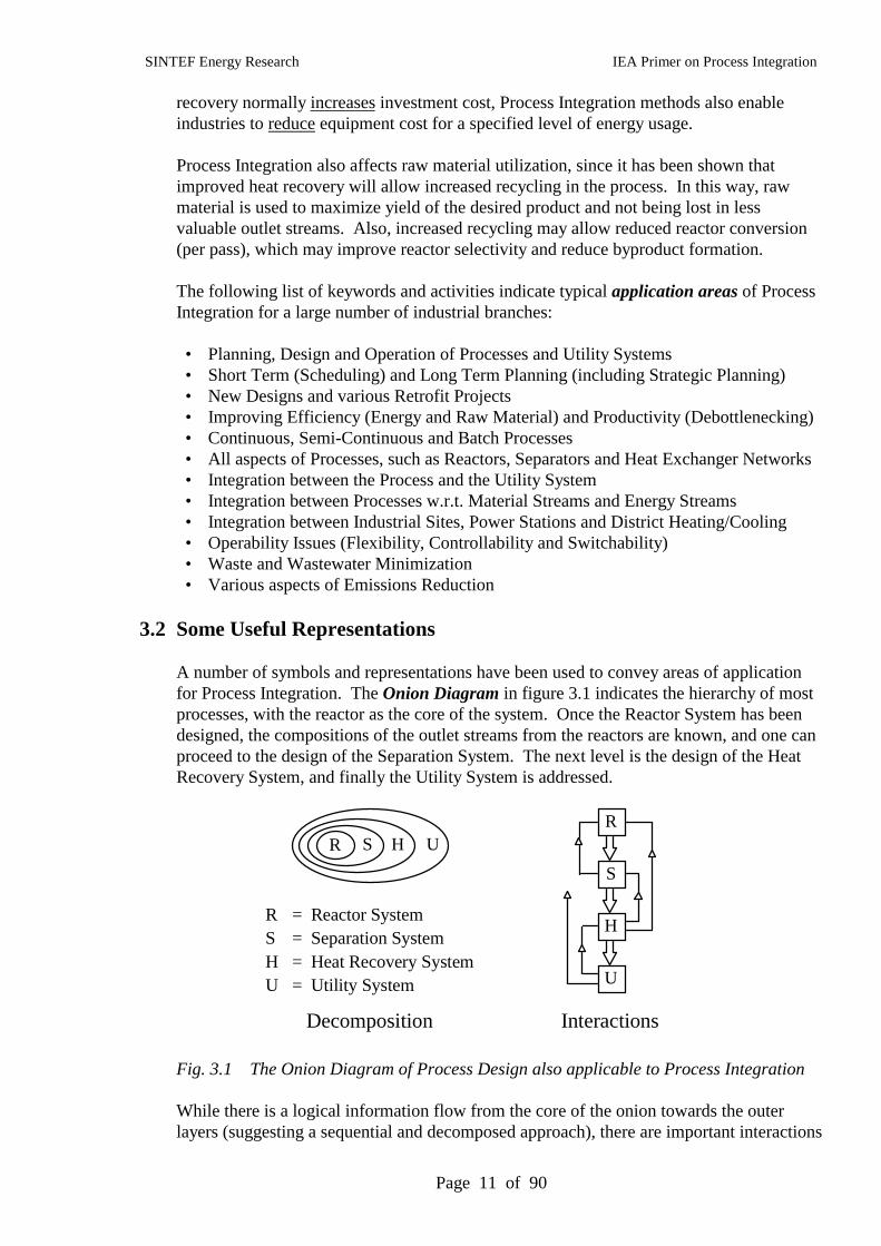
A number of symbols and representations have been used to convey areas of applicationfor Process Integration. The Onion Diagram in figure 3.1 indicates the hierarchy of mostprocesses, with the reactor as the core of the system. Once the Reactor System has beendesigned, the compositions of the outlet streams from the reactors are known, and one canproceed to the design of the Separation System. The next level is the design of the HeatRecovery System, and finally the Utility System is addressed.

R S H U

R = Reactor SystemS = Separation SystemH = Heat Recovery SystemU = Utility System

Decomposition

R

S

H

U

Interactions

Fig. 3.1 The Onion Diagram of Process Design also applicable to Process Integration

While there is a logical information flow from the core of the onion towards the outerlayers (suggesting a sequential and decomposed approach), there are important interactions


Page 12 of 90

that require iteration towards the center of the onion, alternatively a simultaneous approachis required. In addition, there are actually more layers to the onion. One example is totalsites, where several processes interact with each other, and where there normally is acentral utility system for heating, cooling, power, etc. Going even further, one may alsowant to include the community surrounding the plant.

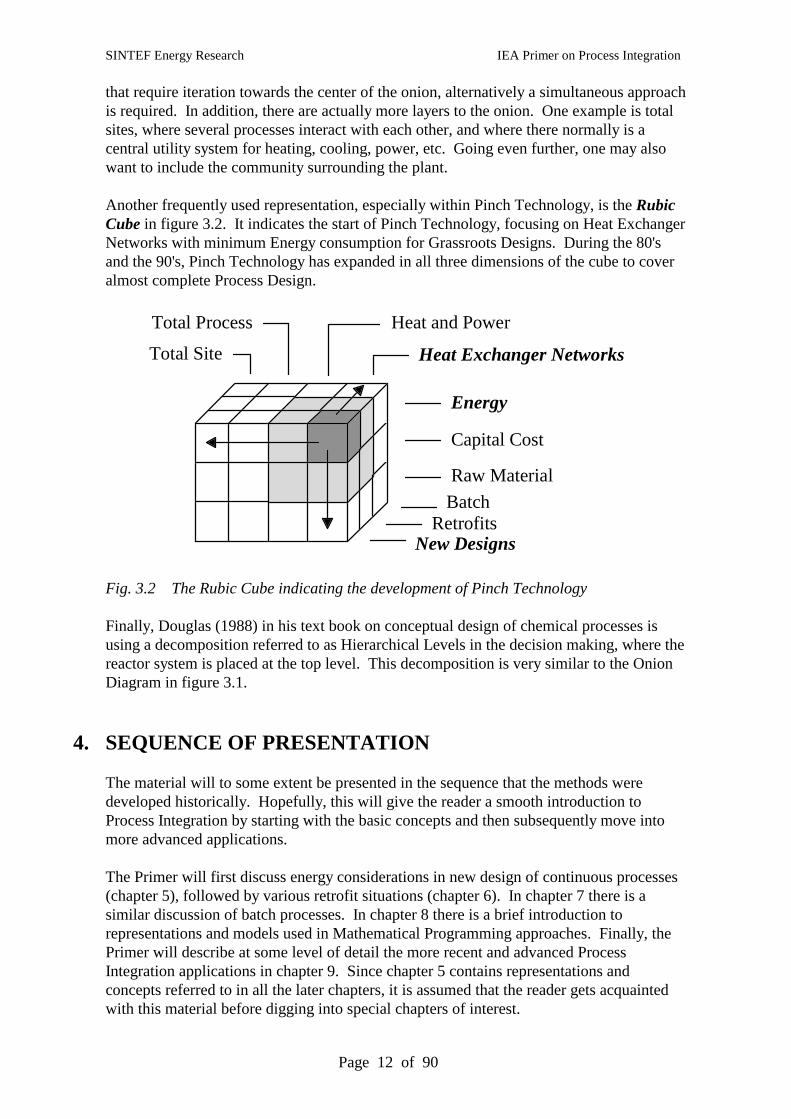
Another frequently used representation, especially within Pinch Technology, is the RubicCube in figure 3.2. It indicates the start of Pinch Technology, focusing on Heat ExchangerNetworks with minimum Energy consumption for Grassroots Designs. During the 80'sand the 90's, Pinch Technology has expanded in all three dimensions of the cube to coveralmost complete Process Design.

Energy

Capital Cost

Raw Material

Heat Exchanger Networks

BatchRetrofits

New Designs

Total Site

Total Process Heat and Power

Fig. 3.2 The Rubic Cube indicating the development of Pinch Technology

Finally, Douglas (1988) in his text book on conceptual design of chemical processes isusing a decomposition referred to as Hierarchical Levels in the decision making, where thereactor system is placed at the top level. This decomposition is very similar to the OnionDiagram in figure 3.1.

4. SEQUENCE OF PRESENTATION

The material will to some extent be presented in the sequence that the methods weredeveloped historically. Hopefully, this will give the reader a smooth introduction toProcess Integration by starting with the basic concepts and then subsequently move intomore advanced applications.

The Primer will first discuss energy considerations in new design of continuous processes(chapter 5), followed by various retrofit situations (chapter 6). In chapter 7 there is asimilar discussion of batch processes. In chapter 8 there is a brief introduction torepresentations and models used in Mathematical Programming approaches. Finally, thePrimer will describe at some level of detail the more recent and advanced ProcessIntegration applications in chapter 9. Since chapter 5 contains representations andconcepts referred to in all the later chapters, it is assumed that the reader gets acquaintedwith this material before digging into special chapters of interest.


Page 13 of 90

5. BASIC CONCEPTS FOR HEAT RECOVERY INNEW DESIGN OF CONTINUOUS PROCESSES

It feels natural to start with the single most important industrial application area forProcess Integration. The development that followed the discovery of the Heat RecoveryPinch has been unique in Process Design when it comes to real life applications inindustry based on results from academic research.

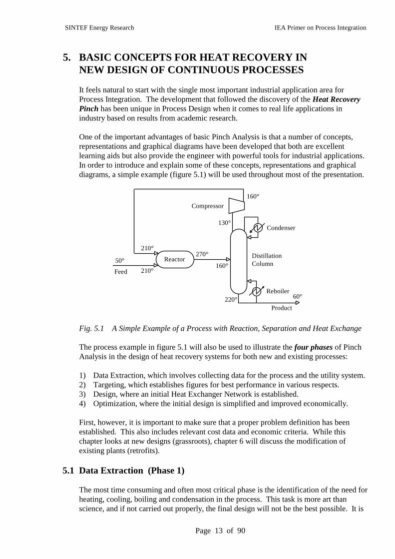
One of the important advantages of basic Pinch Analysis is that a number of concepts,representations and graphical diagrams have been developed that both are excellentlearning aids but also provide the engineer with powerful tools for industrial applications.In order to introduce and explain some of these concepts, representations and graphicaldiagrams, a simple example (figure 5.1) will be used throughout most of the presentation.

Reactor

Feed

Product

DistillationColumn

Compressor

50°

210°

160°

210°

130°

220°

160°

270°

60°Reboiler

Condenser

Fig. 5.1 A Simple Example of a Process with Reaction, Separation and Heat Exchange

The process example in figure 5.1 will also be used to illustrate the four phases of PinchAnalysis in the design of heat recovery systems for both new and existing processes:

1) Data Extraction, which involves collecting data for the process and the utility system.2) Targeting, which establishes figures for best performance in various respects.3) Design, where an initial Heat Exchanger Network is established.4) Optimization, where the initial design is simplified and improved economically.

First, however, it is important to make sure that a proper problem definition has beenestablished. This also includes relevant cost data and economic criteria. While thischapter looks at new designs (grassroots), chapter 6 will discuss the modification ofexisting plants (retrofits).

5.1 Data Extraction (Phase 1)

The most time consuming and often most critical phase is the identification of the need forheating, cooling, boiling and condensation in the process. This task is more art thanscience, and if not carried out properly, the final design will not be the best possible. It is


Page 14 of 90

quite easy to accept too many features of the proposed flowsheet, which inevitably resultsin the situation where many good opportunities are excluded from the analysis.

Once the Data Extraction and corresponding Targeting (Phase 2) activities are completed,it is time to look back and question some of the decisions made for the Reactor andSeparation Systems. The idea is then to identify process modifications that will increasethe potential for heat recovery and/or allow the use of cheaper utilities.

In practice, there are a number of situations where heat integration is not desirable.Examples include long distances (costly piping), safety (heat exchange betweenhydrocarbon streams and oxygen rich streams), product purity (potential leakage in heatexchangers), operability (start-up and shut-down), controllability and flexibility. Areasonable strategy is, however, to start by including all process streams and keep thedegrees of freedom open. Later, practical considerations can be used to exclude some ofthese streams and degrees of freedom, and the engineer will then at any time be able toestablish the consequences with respect to energy consumption and total annual cost.

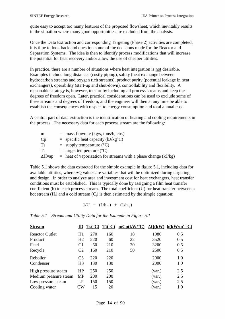
A central part of data extraction is the identification of heating and cooling requirements inthe process. The necessary data for each process stream are the following:

m = mass flowrate (kg/s, tons/h, etc.)Cp = specific heat capacity (kJ/kg°C)Ts = supply temperature (°C)Tt = target temperature (°C)∆Hvap = heat of vaporization for streams with a phase change (kJ/kg)

Table 5.1 shows the data extracted for the simple example in figure 5.1, including data foravailable utilities, where ∆Q values are variables that will be optimized during targetingand design. In order to analyze area and investment cost for heat exchangers, heat transferconditions must be established. This is typically done by assigning a film heat transfercoefficient (h) to each process stream. The total coefficient (U) for heat transfer between ahot stream (Hi) and a cold stream (Cj) is then estimated by the simple equation:

1/U = (1/hHi) + (1/hCj)

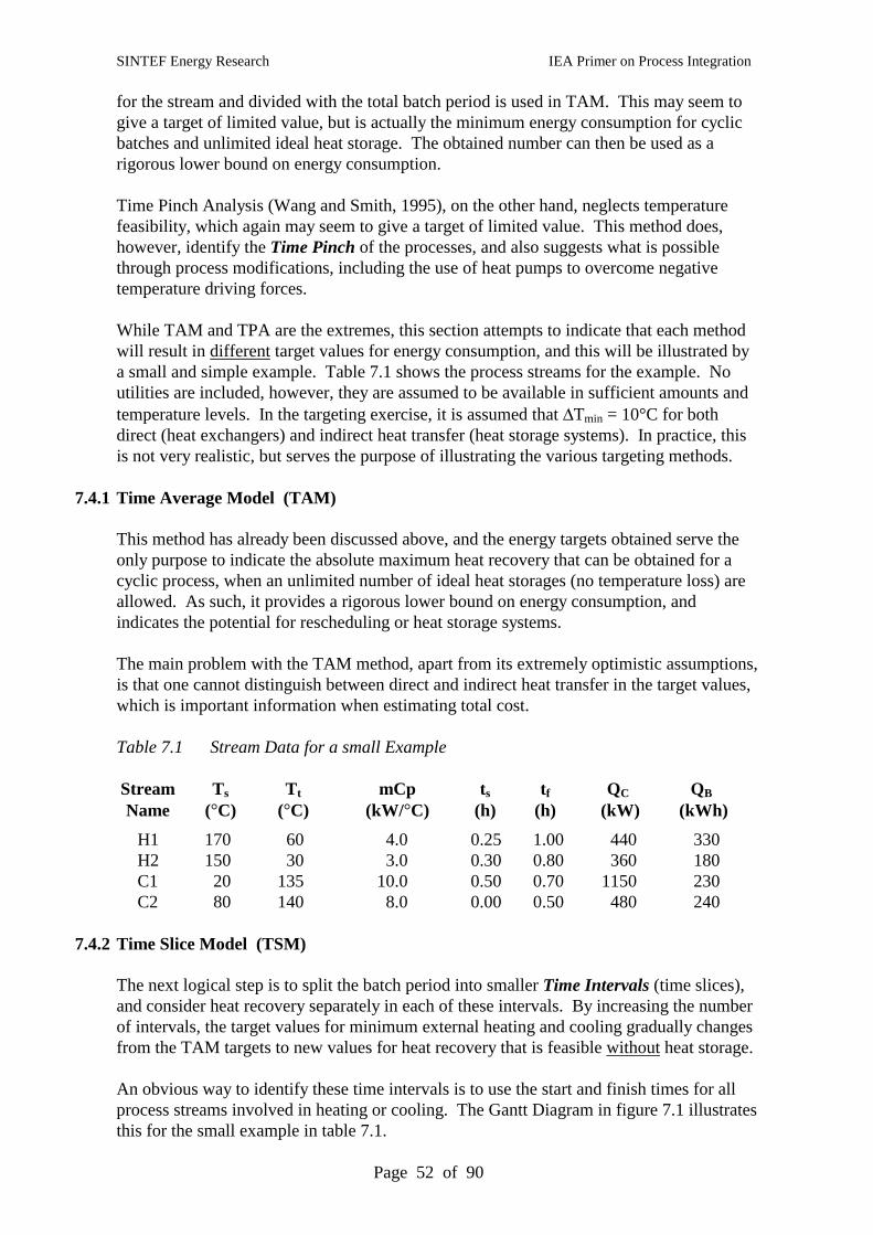
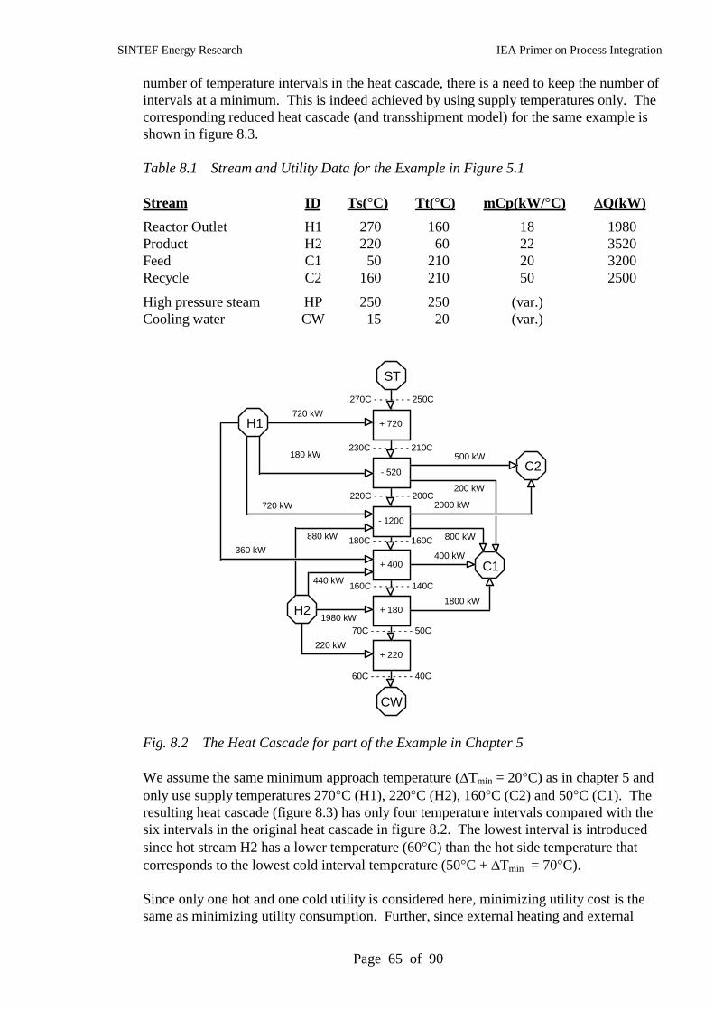
Table 5.1 Stream and Utility Data for the Example in Figure 5.1

Stream ID Ts(°C) Tt(°C) mCp(kW/°C) ∆Q(kW) h(kW/m2 °C)

Reactor Outlet H1 270 160 18 1980 0.5Product H2 220 60 22 3520 0.5Feed C1 50 210 20 3200 0.5Recycle C2 160 210 50 2500 0.5

Reboiler C3 220 220 2000 1.0Condenser H3 130 130 2000 1.0

High pressure steam HP 250 250 (var.) 2.5Medium pressure steam MP 200 200 (var.) 2.5Low pressure steam LP 150 150 (var.) 2.5Cooling water CW 15 20 (var.) 1.0


Page 15 of 90

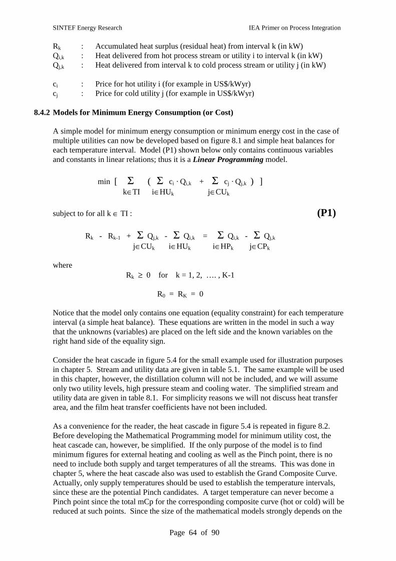
5.2 Performance Targets (Phase 2)

As indicated in section 2.5, an important feature of Process Integration is the ability toidentify Performance Targets before the design phase is started. For heat recovery systemswith a specified value for the minimum allowable approach temperature (∆Tmin), targetscan be established for Minimum Energy Consumption (external heating and cooling),Fewest Number of Units (process/process heat exchangers, heaters and coolers) andMinimum Total Heat Transfer Area. In addition, the corresponding calculations will alsoidentify the Heat Recovery Pinch, which acts as a bottleneck for heat recovery.

For new designs, it is possible to return to data extraction and modify the process in such away that the impact of the heat recovery pinch is reduced or even eliminated. Then a newPinch point will be identified, and the procedure can be repeated.

It is also possible to combine targets for energy, units and total heat transfer area into anestimate of the total annual cost. By repeating these calculations for different values of∆Tmin, it is possible to identify a good starting value for the level of heat recovery. Thisexercise of pre-optimization (Linnhoff and Ahmad, 1990) has been referred to as "Super-Targeting" (which also gave name to one of the commercial software packages available).

While initial methods used a global value for ∆Tmin, later methods allowed individualstream contributions to the overall minimum approach temperature (∆Ti) reflecting theheat transfer conditions for each process stream, as indicated by its film heat transfercoefficient (hi). One model that has been used is ∆Ti = C / sqrt(hi), where C is a commonadjustable factor, reflecting the chosen level of heat recovery (see Ahmad et al., 1990).

5.2.1 Minimum Energy Consumption

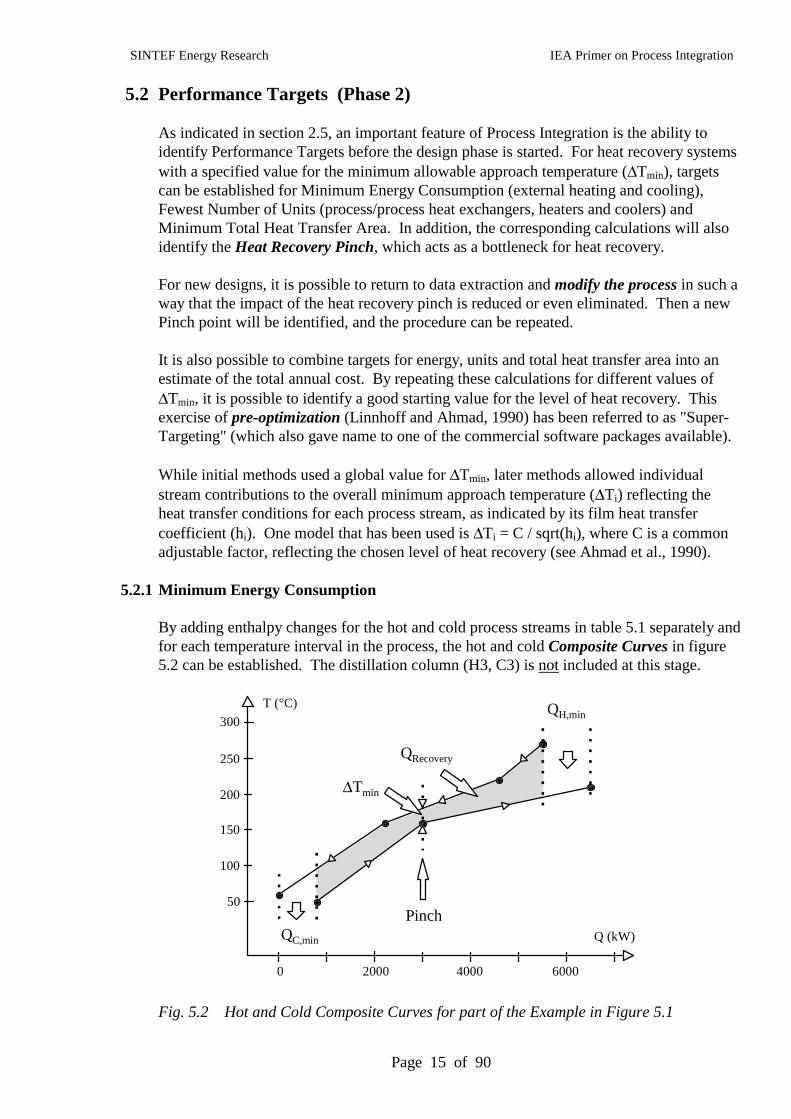
By adding enthalpy changes for the hot and cold process streams in table 5.1 separately andfor each temperature interval in the process, the hot and cold Composite Curves in figure5.2 can be established. The distillation column (H3, C3) is not included at this stage.

300

250

200

150

100

50

T (°C)

Q (kW)

2000 4000 60000

QH,min

QC,min

Pinch

QRecovery

∆Tmin

Fig. 5.2 Hot and Cold Composite Curves for part of the Example in Figure 5.1


Page 16 of 90

Composite Curves provide valuable information about maximum heat recovery (QRecovery),minimum external heating (QH,min), minimum external cooling (QC,min) and location of theheat recovery Pinch for a given value of ∆Tmin. As mentioned in section 2.4, CompositeCurves can be applied and provide valuable information whenever an amount (such asheat) has a quality (such as temperature). The advantages of graphical representations(such as the one in figure 5.2) include a pedagogic aspect of understanding, they providethe engineer with an overview of the problem, they illustrate important economic trade-offs, and finally they represent information in a very concentrated form. The results(targets) that can be extracted from figure 5.2, where ∆Tmin = 20°C, are the following:

Maximum Heat Recovery: QRecovery = 4700 kWMinimum External Heating: QH,min = 1000 kWMinimum External Cooling: QC,min = 800 kWPinch Point (caused by a cold stream): TPinch,C = 160 °CCorresponding Pinch for hot streams: TPinch,H = 180 °C

As indicated in table 5.1, the values for mCp are assumed to be constant. This simplifiesthe calculations from numerical integration to a summation over intervals. When the valueof Cp varies considerably with temperature, introducing stream segments can piece-wiselinearize the temperature/enthalpy relation for the stream. The same applies for a streamthat has a phase change.

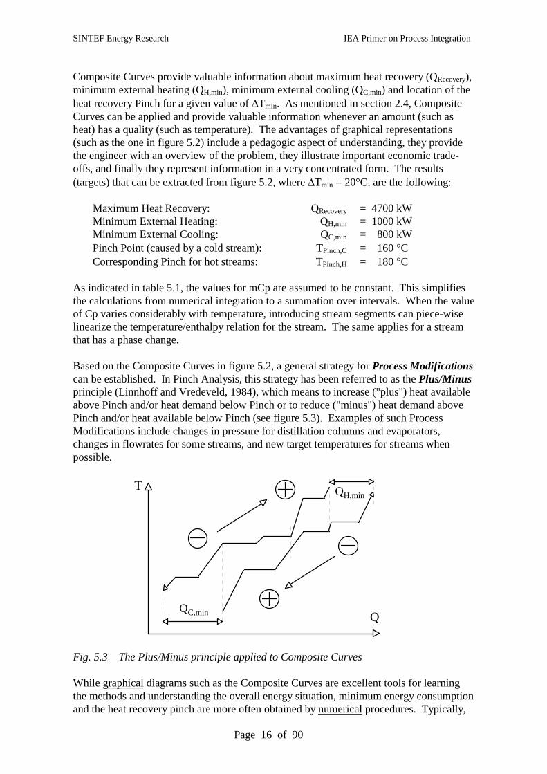
Based on the Composite Curves in figure 5.2, a general strategy for Process Modificationscan be established. In Pinch Analysis, this strategy has been referred to as the Plus/Minusprinciple (Linnhoff and Vredeveld, 1984), which means to increase ("plus") heat availableabove Pinch and/or heat demand below Pinch or to reduce ("minus") heat demand abovePinch and/or heat available below Pinch (see figure 5.3). Examples of such ProcessModifications include changes in pressure for distillation columns and evaporators,changes in flowrates for some streams, and new target temperatures for streams whenpossible.

T

QQC,min

QH,min

Fig. 5.3 The Plus/Minus principle applied to Composite Curves

While graphical diagrams such as the Composite Curves are excellent tools for learningthe methods and understanding the overall energy situation, minimum energy consumptionand the heat recovery pinch are more often obtained by numerical procedures. Typically,


Page 17 of 90

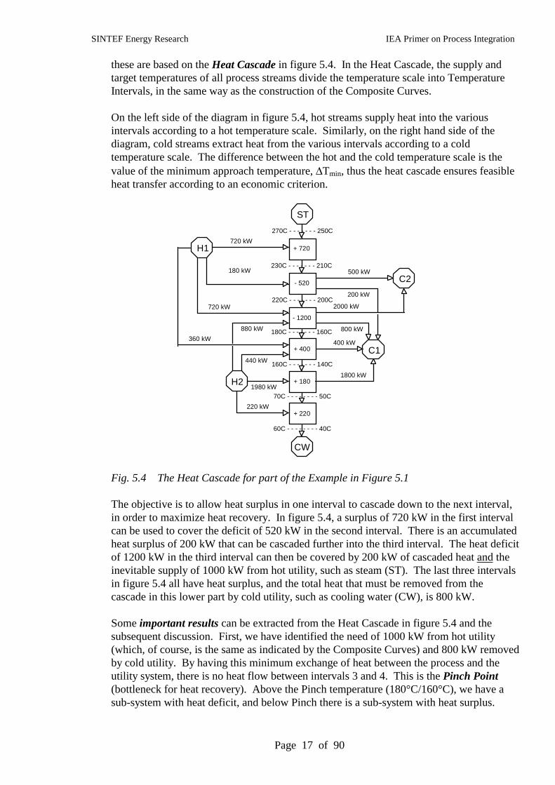
these are based on the Heat Cascade in figure 5.4. In the Heat Cascade, the supply andtarget temperatures of all process streams divide the temperature scale into TemperatureIntervals, in the same way as the construction of the Composite Curves.

On the left side of the diagram in figure 5.4, hot streams supply heat into the variousintervals according to a hot temperature scale. Similarly, on the right hand side of thediagram, cold streams extract heat from the various intervals according to a coldtemperature scale. The difference between the hot and the cold temperature scale is thevalue of the minimum approach temperature, ∆Tmin, thus the heat cascade ensures feasibleheat transfer according to an economic criterion.

270C - - - - - - - 250C

230C - - - - - - - 210C

220C - - - - - - - 200C

180C - - - - - - - 160C

160C - - - - - - - 140C

70C - - - - - - - - 50C

H1

H2

CW

C1

C2

ST

720 kW

180 kW

720 kW

880 kW

440 kW

1980 kW

500 kW

200 kW

800 kW

1800 kW

+ 720

- 520

- 1200

2000 kW

400 kW

+ 180

+ 220

+ 400

60C - - - - - - - - 40C

360 kW

220 kW

Fig. 5.4 The Heat Cascade for part of the Example in Figure 5.1

The objective is to allow heat surplus in one interval to cascade down to the next interval,in order to maximize heat recovery. In figure 5.4, a surplus of 720 kW in the first intervalcan be used to cover the deficit of 520 kW in the second interval. There is an accumulatedheat surplus of 200 kW that can be cascaded further into the third interval. The heat deficitof 1200 kW in the third interval can then be covered by 200 kW of cascaded heat and theinevitable supply of 1000 kW from hot utility, such as steam (ST). The last three intervalsin figure 5.4 all have heat surplus, and the total heat that must be removed from thecascade in this lower part by cold utility, such as cooling water (CW), is 800 kW.

Some important results can be extracted from the Heat Cascade in figure 5.4 and thesubsequent discussion. First, we have identified the need of 1000 kW from hot utility(which, of course, is the same as indicated by the Composite Curves) and 800 kW removedby cold utility. By having this minimum exchange of heat between the process and theutility system, there is no heat flow between intervals 3 and 4. This is the Pinch Point(bottleneck for heat recovery). Above the Pinch temperature (180°C/160°C), we have asub-system with heat deficit, and below Pinch there is a sub-system with heat surplus.


Page 18 of 90

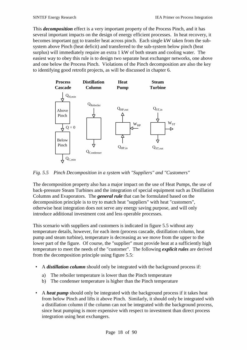
This decomposition effect is a very important property of the Process Pinch, and it hasseveral important impacts on the design of energy efficient processes. In heat recovery, itbecomes important not to transfer heat across pinch. Each single kW taken from the sub-system above Pinch (heat deficit) and transferred to the sub-system below pinch (heatsurplus) will immediately require an extra 1 kW of both steam and cooling water. Theeasiest way to obey this rule is to design two separate heat exchanger networks, one aboveand one below the Process Pinch. Violations of the Pinch decomposition are also the keyto identifying good retrofit projects, as will be discussed in chapter 6.

AbovePinch

BelowPinch

QH,min

QC,min

Q = 0

ProcessCascade

QReboiler

QCondenser

DistillationColumn

HeatPump

QHP,out

QHP,in

WHP

SteamTurbine

QST,in

QST,out

WST

Fig. 5.5 Pinch Decomposition in a system with "Suppliers" and "Customers"

The decomposition property also has a major impact on the use of Heat Pumps, the use ofback-pressure Steam Turbines and the integration of special equipment such as DistillationColumns and Evaporators. The general rule that can be formulated based on thedecomposition principle is to try to match heat "suppliers" with heat "customers",otherwise heat integration does not serve any energy saving purpose, and will onlyintroduce additional investment cost and less operable processes.

This scenario with suppliers and customers is indicated in figure 5.5 without anytemperature details, however, for each item (process cascade, distillation column, heatpump and steam turbine), temperature is decreasing as we move from the upper to thelower part of the figure. Of course, the "supplier" must provide heat at a sufficiently hightemperature to meet the needs of the "customer". The following explicit rules are derivedfrom the decomposition principle using figure 5.5:

• A distillation column should only be integrated with the background process if:

a) The reboiler temperature is lower than the Pinch temperatureb) The condenser temperature is higher than the Pinch temperature

• A heat pump should only be integrated with the background process if it takes heatfrom below Pinch and lifts it above Pinch. Similarly, it should only be integrated witha distillation column if the column can not be integrated with the background process,since heat pumping is more expensive with respect to investment than direct processintegration using heat exchangers.


Page 19 of 90

• A steam turbine should only be integrated (i.e. back pressure or extraction turbine)with a process or distillation column if the outlet steam has a high enough condensingtemperature (high enough pressure) to be used above the process Pinch or in a columnreboiler. Otherwise a condensing turbine should be used.

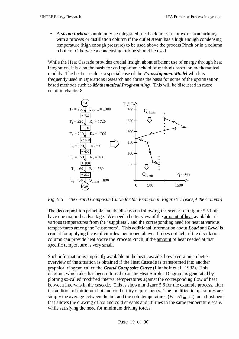
While the Heat Cascade provides crucial insight about efficient use of energy through heatintegration, it is also the basis for an important school of methods based on mathematicalmodels. The heat cascade is a special case of the Transshipment Model which isfrequently used in Operations Research and forms the basis for some of the optimizationbased methods such as Mathematical Programming. This will be discussed in moredetail in chapter 8.

300

250

200

150

100

50

T (°C)

Q (kW)

500 15000

QH,min

QC,min

CW

ST

+ 720

- 520

- 1200

+ 180

+ 220

+ 400

T0 = 260 QH,min = 1000

T1 = 220 R1 = 1720

T2 = 210 R2 = 1200

T3 = 170 R3 = 0

T4 = 150 R4 = 400

T5 = 60 R5 = 580

T6 = 50 QC,min = 800

Fig. 5.6 The Grand Composite Curve for the Example in Figure 5.1 (except the Column)

The decomposition principle and the discussion following the scenario in figure 5.5 bothhave one major disadvantage. We need a better view of the amount of heat available atvarious temperatures from the "suppliers", and the corresponding need for heat at varioustemperatures among the "customers". This additional information about Load and Level iscrucial for applying the explicit rules mentioned above. It does not help if the distillationcolumn can provide heat above the Process Pinch, if the amount of heat needed at thatspecific temperature is very small.

Such information is implicitly available in the heat cascade, however, a much betteroverview of the situation is obtained if the Heat Cascade is transformed into anothergraphical diagram called the Grand Composite Curve (Linnhoff et al., 1982). Thisdiagram, which also has been referred to as the Heat Surplus Diagram, is generated byplotting so-called modified interval temperatures against the corresponding flow of heatbetween intervals in the cascade. This is shown in figure 5.6 for the example process, afterthe addition of minimum hot and cold utility requirements. The modified temperatures aresimply the average between the hot and the cold temperatures (+/- ∆Tmin /2), an adjustmentthat allows the drawing of hot and cold streams and utilities in the same temperature scale,while satisfying the need for minimum driving forces.


Page 20 of 90

The Grand Composite Curve has a number of industrial applications, mostly related to theutility system and heat and power considerations. Typically, the Grand Composite Curvecan be used to qualitatively and to some extent quantitatively address the following tasks:

• Identify a near-optimal set of utility types (both load and level) to cover the need forexternal heating and cooling in the process. A Utility Grand Composite Curve (Hall,1989) consisting of available utilities, such as for example various steam levels, fluegas from a furnace or gas turbine, hot oil circuits, cooling water, refrigeration, etc., canbe combined in such a way that total utility cost is minimized.

• Identify potential for steam production below Pinch, if the process Pinch is at asufficiently high temperature. This means that steam generation (typically LP steam)is acting as a cold utility.

• Identify potential for utilizing so-called "pockets" in the Grand Composite Curve foradditional power production. There is one such pocket above Pinch in figure 5.6. Ifthe temperature difference had been sufficiently large between the part of the processwhere there is local heat surplus and the corresponding part where there is local heatdeficit, there would have been some scope for producing steam that could have beenused in a back pressure turbine. The turbine then borrows steam generated in theprocess and returns steam for heating at a lower level after power production.

• Identify scope for using heat pumps in the process to reduce both hot and cold utilityconsumption. Typically, this is the case where there is a distinct Pinch point, with flatprofiles both immediately above and below the Pinch. In such cases, a significantamount of heat can be transferred from the heat surplus region below Pinch to the heatdeficit region above Pinch, by using a heat pump with moderate temperature lift.

• Identify whether there is scope for integration of special equipment such asdistillation columns or evaporators with the background process.

300

250

200

150

100

50

T (°C)

Q (kW)

1000 20000

QH,min

QC,min

3000

QReboiler

QCondenser

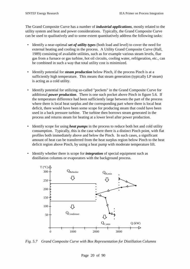
Fig. 5.7 Grand Composite Curve with Box Representation for Distillation Columns


Page 21 of 90

Returning to the process example in figure 5.1, the Grand Composite Curve can be used togive a quick and simple answer about the scope for integrating the distillation columnwith the background process, or whether it should be operated with utilities (steam andcooling water). After heat integration with the process has been analyzed, the next stepcould be to evaluate the scope for heat pumping.

Figure 5.7 shows the Process Grand Composite Curve and the Temperature/EnthalpyDiagram for the distillation column in figure 5.1. Since the distillation column operatesacross the Pinch, there will be no energy savings from integration with the process. Thisalso follows from the decomposition concept illustrated in figure 5.5. The graphicalrepresentation in figure 5.7 has also been referred to as the Andrecovich diagram.

Later extensions within Pinch Analysis include a refinement of the box representation,where a Column Grand Composite Curve (CGCC) shows the need for reboiling andcondensation at various temperatures in the column. The CGCC is based on convergedprofiles from a rigorous column simulation, and can be used to identify the scope fordistributed reboiling and condensing as well as feed pre-heating or pre-cooling, and finallychanges in the reflux ratio for the column.

300

250

200

150

100

50

T (°C)

Q (kW)

500 15000

MP

HP

0

LP

CW

Consumption:

HP: 400 kWMP: 600 kWCW: 600 kW

Production:

LP: 200 kW

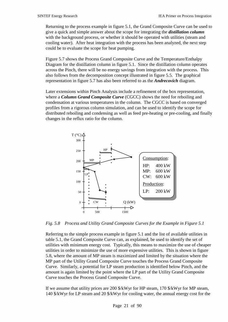
Fig. 5.8 Process and Utility Grand Composite Curves for the Example in Figure 5.1

Referring to the simple process example in figure 5.1 and the list of available utilities intable 5.1, the Grand Composite Curve can, as explained, be used to identify the set ofutilities with minimum energy cost. Typically, this means to maximize the use of cheaperutilities in order to minimize the use of more expensive utilities. This is shown in figure5.8, where the amount of MP steam is maximized and limited by the situation where theMP part of the Utility Grand Composite Curve touches the Process Grand CompositeCurve. Similarly, a potential for LP steam production is identified below Pinch, and theamount is again limited by the point where the LP part of the Utility Grand CompositeCurve touches the Process Grand Composite Curve.

If we assume that utility prices are 200 $/kWyr for HP steam, 170 $/kWyr for MP steam,140 $/kWyr for LP steam and 20 $/kWyr for cooling water, the annual energy cost for the


Page 22 of 90

utility mix in figure 5.8 is 166,000 $/yr. When using HP steam and cooling water only, thecorresponding annual energy cost is 216,000 $/yr, i.e. 30% higher.

The Grand Composite Curve enables the engineer to identify a set of utilities that givesminimum energy cost. As always, however, there is a trade-off between operating cost(energy) and investment cost (number of heat exchangers and their total heat transfer area).Thus, the following important factors need further investigation before accepting the set ofutilities proposed in figure 5.8:

• Temperature driving forces will be reduced when introducing MP and LP steam,which means larger heat transfer area in some utility and process/process exchangers.As a result, there will be a significant increase in the investment cost.

• New Utility Pinch Points will be introduced when maximizing MP steam usage andLP steam production. This will result in tighter designs and more complex heatexchanger network structures.

• The decomposition feature of the Process Pinch also applies to Utility Pinches. Thismeans for example that heat pumps can be used to transfer heat across (from below toabove) all Pinch points in order to reduce total heating and cooling requirements(Process Pinch) or reduce the need for a more expensive utility (Utility Pinch).

• The number of heat transfer units will increase whenever new utilities are introducedand whenever Utility Pinches are created, which means increased investment cost.

• The complexity of the heat exchanger network (number of units, piping and streamsplits) will increase with an increasing number of Pinch points included during design.

While significant savings in energy cost can be obtained by introducing intermediate (andthus cheaper) utilities, there will be a corresponding increase in investment cost (total heattransfer area and the number of units will increase). Minimum total annual cost is foundby exploring these trade-offs.

The Grand Composite Curve (GCC) has the inherent limitation (which also in manyrespects is an advantage) that details about the individual streams are not shown. Thus,any conclusion about integration of distillation columns and heat pumps as well as steamgeneration, must be evaluated carefully by looking beyond the GCC and into the actualnumber of streams that would be involved. If a heat pump would have to extract (deliver)heat from (to) a large number of streams, it would not be economically interesting. Thesame applies if we end up with a large number of steam boilers.

5.2.2 Fewest Number of Units

A heuristic estimate for the minimum number of units is obtained by using Euler's Rulefrom Graph Theory as the basis:

U = N + L - S

where U is the number of units (process/process heat exchangers, heaters and coolers), N isthe total number of process streams and utility types, L is the number of heat load loops in


Page 23 of 90

the network and S is the number of sub-systems in the network. Assuming there are noheat load loops (it will be shown later that loops can be removed) and no sub-networks(sets of hot and cold streams in perfect heat balance, which would be a coincidence), thefollowing can be used as an estimate for the fewest number of units:

Umin = N + 0 - 1 = N - 1

In order to obtain Maximum Energy Recovery (MER) or minimum energy consumption,however, it was shown above that decomposition at the Process Pinch must be respected.This means that separate heat exchanger networks must be designed above and belowPinch, and the corresponding minimum total number of units is given by:

Umin,MER = ( N - 1 )above + ( N - 1 )below

In the case of multiple utilities, as indicated in figure 5.8, new Utility Pinch points will beintroduced whenever a cheaper utility is maximized in order to minimize a more expensiveutility. There are also cases with near-Pinches that could be included to make tight designsituations easier. A more general equation for the fewest number of units is thus:

Umin,MER = ( Ni - 1)Σi=1

np+1

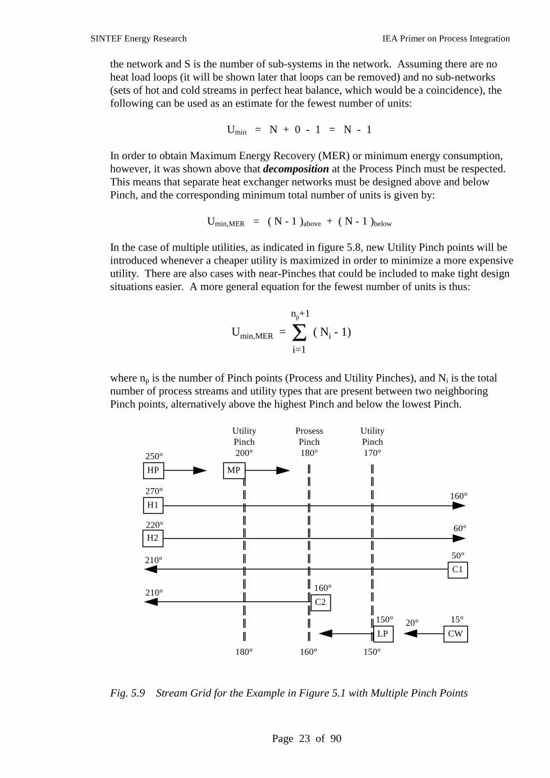
where np is the number of Pinch points (Process and Utility Pinches), and Ni is the totalnumber of process streams and utility types that are present between two neighboringPinch points, alternatively above the highest Pinch and below the lowest Pinch.

ProsessPinch180°

C2210° 160°

C1210° 50°

H2

220° 60°

H1

270° 160°

160°

HP

250°

MP

180°

LP

150°

CW

15°

150°

UtilityPinch200°

UtilityPinch170°

20°

Fig. 5.9 Stream Grid for the Example in Figure 5.1 with Multiple Pinch Points


Page 24 of 90

It is obvious from these equations that the target for minimum number of units depends onthe number of utility types that are used and the number of Pinch points (process andutility pinches) where strict decomposition is implemented. For the simple example infigure 5.1 with 4 process streams (keeping the distillation column out of the discussion)and up to 4 utility types, the fewest number of units varies considerably. If we only use HPand CW and do not decompose at the process Pinch, the fewest number of units is 4, whileit is 14 if we use all 4 utility types and decompose at all 3 Pinch points. Obviously, theeconomic trade-off between energy cost and equipment cost will have an optimum that iscloser to 5 heat transfer units than 14.

The Stream Grid (Linnhoff and Flower, 1978a) shown in figure 5.9 is an importantrepresentation for the design of heat exchanger networks. It can also be used to assist inthe application of the (N-1) rule to calculate the fewest number of heat exchangers for thevarious scenarios of multiple utilities and the existence of Process and Utility Pinch points.

5.2.3 Minimum Number of Shells

Refinements have been made in Pinch Analysis (Ahmad and Smith, 1989) to reflect thefact that very few industrial heat exchangers are pure counter-current. These refinementsrelate to both the number of heat exchange units (now counted as number of shells ratherthan heat exchangers) and to heat transfer area (see the discussion in section 5.2.4).

So far, these extensions only apply to Shell & Tube exchangers, where correction factorsfor heat transfer area (fT) are used that depend on mCp values and temperatures for thestreams. These factors represent deviations from pure counter-current heat exchange whenusing models and equations for 1-2 Shell & Tube exchangers. If the value of fT falls undera minimum acceptable value, the number of shells must be increased by one, and theprocedure is repeated. With these extended models, it is possible to obtain a target for theminimum number of shells rather than units. The next section on minimum heat transferarea also applies to shells in 1-2 configurations, with the addition of the fT factor whencalculating area.

5.2.4 Minimum Heat Transfer Area

Estimating the need for total heat transfer area in the network of heat exchangers beforedesign is both the most time consuming (need software) and the most uncertain targetingactivity. There are large uncertainties in heat transfer coefficients, and simplifiedassumptions are made about the network structure when calculating minimum total area.

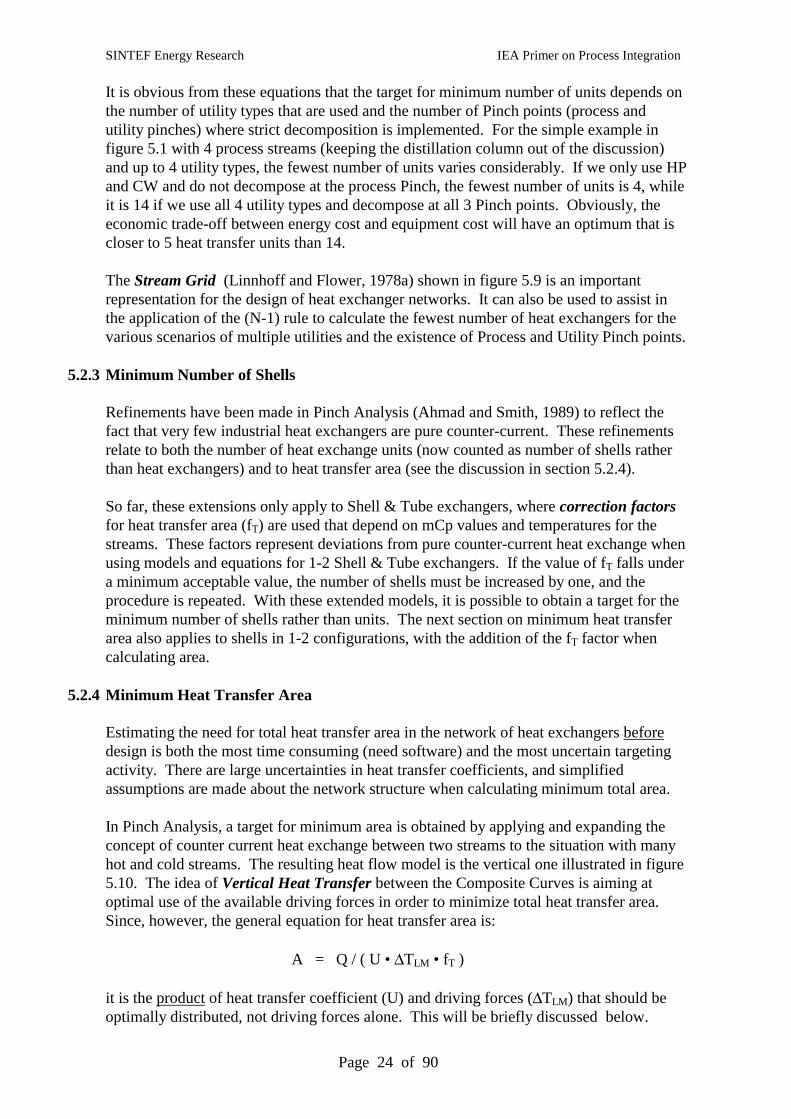
In Pinch Analysis, a target for minimum area is obtained by applying and expanding theconcept of counter current heat exchange between two streams to the situation with manyhot and cold streams. The resulting heat flow model is the vertical one illustrated in figure5.10. The idea of Vertical Heat Transfer between the Composite Curves is aiming atoptimal use of the available driving forces in order to minimize total heat transfer area.Since, however, the general equation for heat transfer area is:

A = Q / ( U • ∆TLM • fT )

it is the product of heat transfer coefficient (U) and driving forces (∆TLM) that should beoptimally distributed, not driving forces alone. This will be briefly discussed below.


Page 25 of 90

300

250

200

150

100

50

T (°C)

Q (kW)

2000 4000 60000

CW

HP

Fig. 5.10 Vertical Heat Transfer for the Example in Figure 5.1

In order to achieve vertical heat transfer in a heat exchanger network, however, all heatexchangers in the same Enthalpy Interval (marked by the dotted lines in figure 5.10) musthave exactly the same temperature profiles. This can only be achieved by considerablesplitting and mixing of streams and a large number of small heat exchangers (must applythe N-1 rule to each enthalpy interval). The corresponding network is therefore referred toas the "Spaghetti Design", and serves exclusively as a calculation model for total heattransfer area (Townsend and Linnhoff, 1984).

In figure 5.10, hot and cold utilities are included and the result is often referred to as theBalanced Composite Curves. In this case only HP steam and cooling water are used. Theactual calculation of minimum area, based on the concept of vertical heat transfer, is donewith the so-called Bath formulae (after the place where the equation was presented):

Amin = Σj ( 1 / ∆TLM, j ) Σi (qi) / (hi)

where qi is the change in enthalpy and hi is the film heat transfer coefficient for stream (i)in enthalpy interval (j). By applying this equation to the example problem we get thefollowing results:

With MP/LP: Amin = 775 m2 Without MP/LP: Amin = 632 m2

Thus, while the introduction of MP and LP steam reduces total energy cost with about30%, there is an increase in the target for heat transfer area of about 23%. In addition, asdiscussed in the previous section, there will be an increase in the number of units, and thenetwork structure will be more complex.

As mentioned above, there are a number of uncertainties related to these target values forminimum area. In addition to the fact that heat transfer coefficients are uncertain bynature, the vertical model and the Bath equation have two severe limitations:


Page 26 of 90

• To achieve minimum area, a large number of heat exchangers, splitters and mixers arerequired. Due to economy of scale effects, cost optimal heat exchanger networks willhave close to the fewest number of units rather than close to minimum area. The so-called Spaghetti Design should only be regarded as a model for calculating Amin.

• The strict vertical model will only result in minimum area if all film heat transfercoefficients for the hot streams area equal (hH), and that all cold stream film heattransfer coefficients are equal (hC). With significant differences in these coefficients,streams with low film heat transfer coefficients should be matched and allowed moredriving forces at the expense of matches between streams with large film heat transfercoefficients that will be assigned less driving forces. As a result, there may beconsiderable non-vertical (Criss-Cross) heat transfer.

These limitations are important, however, the main use of the target for minimum area is tobe able to estimate total annual cost ahead of design for various values of ∆Tmin, in order toidentify a good starting point for the design exercise.

5.2.5 Total Annual Cost

By combining targets for minimum energy consumption, fewest number of units or shellsand minimum heat transfer area, as well as cost data for utilities, cost equations for heatexchangers, some economic factors such as payback time or interest rate, and the numberof operating hours per year, it is possible to obtain figures for Total Annual Cost. Thereare also uncertainties in these estimates, for example related to the fact that we only havefigures for total area, and not how this area is distributed among the heat exchangers. Withan economy of scale type cost equation, such a distribution is important for the final result.

Experience from industrial projects have shown, however, that some of the uncertaintiesand assumptions in the calculation of area and total annual cost tend to cancel, and that theestimated total cost often is within a few percent from the total cost of the final heatexchanger network (using the same cost and economic data).

As mentioned above, the main purpose of estimating Total Annual Cost (TAC) is toidentify a good starting point for network design. This is done by calculating the differenttargets and the resulting total annual cost for various values of ∆Tmin. By selecting a valuefor ∆Tmin where TAC has a minimum, the initial heat exchanger network (see next section)will have a structure that is compatible with the final optimal network.

In the case of multiple utilities, a similar economic trade-off should be explored in thetargeting phase. Methods have been developed within Pinch Analysis that can be used toidentify near-optimal amounts of the various utilities (Parker, 1989, and Hall et al., 1992).It should also be mentioned that utility selection and process modifications interact andmust be considered simultaneously.

5.3 Network Design (Phase 3)

This section will be presented in much less detail than the previous section where anumber of concepts, representations and graphical diagrams were introduced that are of ageneral nature with several different applications in Process Integration.


Page 27 of 90

Design of Heat Exchanger Networks in various industries is primarily carried out using thenow classical Pinch Design Method (Linnhoff and Hindmarsh, 1983). While the originalmethod focused on minimum energy consumption and the fewest number of units, latergraphical and numerical additions made it possible also to consider heat transfer area andtotal annual cost during design. Both the original features and the later extensions havebeen implemented in current state of the art commercial software packages for HeatExchanger Network Design.

The basic Pinch Design Method respects the decomposition at Process and Utility Pinchpoints and provides a strategy and matching rules that enable the engineer to obtain aninitial network, which achieves the minimum energy target. The Stream Grid presented insection 5.2.2 is very useful in the design phase and acts as a drawing board, where theengineer places one match at a time using these matching rules. The Pinch Design Methodalso indicates situations where stream splitting is required to reach the minimum energytarget. Stream splitting is also important in area considerations and the optimal use oftemperature driving forces.

The design strategy mentioned above is simply to start design at the Pinch, where drivingforces are limited and the critical matches for maximum heat recovery must be selected.The matching rules simply ensure sufficient driving forces, and they attempt to minimizethe number of units. The design then gradually moves away from the pinch, making surethat hot streams are utilized above Pinch (limited resource), and vice versa for cold streamsbelow Pinch (limited resource).

The matching rules for Pinch exchangers (those situated immediately above or belowPinch) can be expressed mathematically by (where Hi and Cj are potential streams to bematched in a heat exchanger):

Above Pinch Below Pinch

mCpCj ≥ mCpHi mCpHi ≥ mCpCj

nC ≥ nH nH ≥ nC

Making sure that every unit fully satisfies the enthalpy change of either the hot or the coldstream (the “tick-off” rule) minimizes the number of units. If the inequalities above arenot satisfied for a complete set of Pinch exchangers, stream splitting has to be consideredin order to reach Maximum Energy Recovery (MER). It is always possible by streamsplitting to satisfy all the inequalities, since total mCp for cold streams are larger than totalmCp for hot streams above Pinch, and vice versa below Pinch.

Later extensions enable the engineer to also consider investment cost during design, inparticular the effect of each match on total heat transfer area. The Driving Force Plot(Linnhoff and Vredeveld, 1984) makes is possible to evaluate graphically whether asuggested match is using reasonable driving forces compared with what is available in thattemperature region of the process.

The Remaining Problem Analysis (Ahmad, 1985) is more quantitative tool, that providesfigures for energy (E), number of units (U), heat transfer area (A) and total annual cost(TAC), if a suggested match is accepted. Adding actual figures for partial designs underdevelopment to target values for the remaining problem provides accumulated figures forTAC.


Page 28 of 90

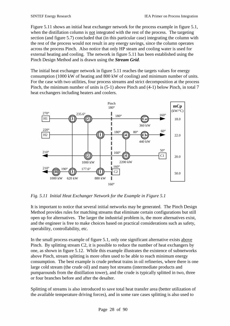
Figure 5.11 shows an initial heat exchanger network for the process example in figure 5.1,when the distillation column is not integrated with the rest of the process. The targetingsection (and figure 5.7) concluded that (in this particular case) integrating the column withthe rest of the process would not result in any energy savings, since the column operatesacross the process Pinch. Also notice that only HP steam and cooling water is used forexternal heating and cooling. The network in figure 5.11 has been established using thePinch Design Method and is drawn using the Stream Grid.

The initial heat exchanger network in figure 5.11 reaches the targets values for energyconsumption (1000 kW of heating and 800 kW of cooling) and minimum number of units.For the case with two utilities, four process streams and strict decomposition at the processPinch, the minimum number of units is (5-1) above Pinch and (4-1) below Pinch, in total 7heat exchangers including heaters and coolers.

Pinch180°

C2210° 160°

C1210° 50°

H2

220° 60°

H1

270° 160°

160°

Ca

4

4

H

1

13

3

2

2

190° 177.6°

1000 kW

1000 kW 620 kW 880 kW

Cb

360 kW

440 kW

2200 kW

160°

180°

180°

80°

235.6°

mCp(kW/°C)

18.0

22.0

20.0

50.0

Fig. 5.11 Initial Heat Exchanger Network for the Example in Figure 5.1

It is important to notice that several initial networks may be generated. The Pinch DesignMethod provides rules for matching streams that eliminate certain configurations but stillopen up for alternatives. The larger the industrial problem is, the more alternatives exist,and the engineer is free to make choices based on practical considerations such as safety,operability, controllability, etc.

In the small process example of figure 5.1, only one significant alternative exists abovePinch. By splitting stream C2, it is possible to reduce the number of heat exchangers byone, as shown in figure 5.12. While this example illustrates the existence of subnetworksabove Pinch, stream splitting is more often used to be able to reach minimum energyconsumption. The best example is crude preheat trains in oil refineries, where there is onelarge cold stream (the crude oil) and many hot streams (intermediate products andpumparounds from the distillation tower), and the crude is typically splitted in two, threeor four branches before and after the desalter.

Splitting of streams is also introduced to save total heat transfer area (better utilization ofthe available temperature driving forces), and in some rare cases splitting is also used to


Page 29 of 90

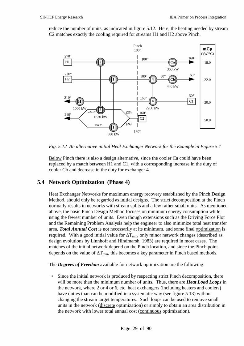
reduce the number of units, as indicated in figure 5.12. Here, the heating needed by streamC2 matches exactly the cooling required for streams H1 and H2 above Pinch.

Pinch180°

C2210° 160°

C1210° 50°

H2

220° 60°

H1

270° 160°

160°

Ca

4

4

H

196.7°

222.3°2

2

1620 kW

1000 kW

1

1

880 kW

Cb

360 kW

440 kW

2200 kW

160°

180°

180°

80°

mCp(kW/°C)

18.0

22.0

20.0

50.0

(26)

(24)

Fig. 5.12 An alternative initial Heat Exchanger Network for the Example in Figure 5.1

Below Pinch there is also a design alternative, since the cooler Ca could have beenreplaced by a match between H1 and C1, with a corresponding increase in the duty ofcooler Cb and decrease in the duty for exchanger 4.

5.4 Network Optimization (Phase 4)

Heat Exchanger Networks for maximum energy recovery established by the Pinch DesignMethod, should only be regarded as initial designs. The strict decomposition at the Pinchnormally results in networks with stream splits and a few rather small units. As mentionedabove, the basic Pinch Design Method focuses on minimum energy consumption whileusing the fewest number of units. Even though extensions such as the Driving Force Plotand the Remaining Problem Analysis help the engineer to also minimize total heat transferarea, Total Annual Cost is not necessarily at its minimum, and some final optimization isrequired. With a good initial value for ∆Tmin, only minor network changes (described asdesign evolutions by Linnhoff and Hindmarsh, 1983) are required in most cases. Thematches of the initial network depend on the Pinch location, and since the Pinch pointdepends on the value of ∆Tmin, this becomes a key parameter in Pinch based methods.

The Degrees of Freedom available for network optimization are the following:

• Since the initial network is produced by respecting strict Pinch decomposition, therewill be more than the minimum number of units. Thus, there are Heat Load Loops inthe network, where 2 or 4 or 6, etc. heat exchangers (including heaters and coolers)have duties than can be modified in a systematic way (see figure 5.13) withoutchanging the stream target temperatures. Such loops can be used to remove smallunits in the network (discrete optimization) or simply to obtain an area distribution inthe network with lower total annual cost (continuous optimization).


Page 30 of 90

• There will also be Heat Load Paths from a hot utility exchanger through some of theprocess/process exchangers to a cold utility exchanger. These paths can be used torestore unacceptable temperature driving forces in some units after manipulation ofheat load loops. Since increasing the duties of utility exchangers will affect theenergy/area trade-off, this procedure has similarities to shifting the Composite Curvesfor the overall problem. A heat load path, however, affects only a limited number ofunits. In some cases, such heat load paths can also be used to remove small units.

• Flowrates of the individual branches of a Stream Split can be varied in order to reducetotal heat transfer area (or actually investment cost) of the heat exchangers involved.This is a local optimization affecting a limited number of units, but interactions existbetween this optimization and the manipulation of heat load loops and paths.

Figure 5.13 shows a Heat Load Loop in the initial heat exchanger network from figure5.11, involving all four process/process exchangers. Another heat load loop existsbetween the two process/process exchangers 2 and 4 and the two coolers Ca and Cb. Infigure 5.13, it is possible to remove exchanger 1 by selecting X = 880 kW or to removeexchanger 3 by selecting X = - 620 kW.

Pinch180°

C2210° 160°

C1210° 50°

H2

220° 60°

H1

270° 160°

160°

Ca

4

4

H

1

13

3

2

2

Cb

620 + X 880 - X

2200 + X1000 - X

T1

T2

T3

T4

Fig. 5.13 Heat Load Loop in the initial Heat Exchanger Network

With economy of scale type cost equations, the obvious strategy is to remove small units,since these are expensive in terms of cost for the given heat recovered ($/kW). Theseeffects are illustrated by the following cost equation:

Chex = a + b • ( A ) c

where (a) is the fixed charge term, (b) is the cost factor for heat transfer area (A), and (c) isthe area exponent which typically is less than 1.0 ("economy of scale").

A Heat Load Path from the heater (H) to one of the coolers (Cb) is illustrated in figure5.14. This network is the result after removing heat exchanger (1) from the network infigure 5.13. As shown in figure 5.14, heat exchanger (2) has infeasible driving forces in


Page 31 of 90

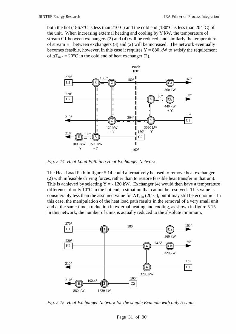
both the hot (186.7ºC is less than 210ºC) and the cold end (180°C is less than 204°C) ofthe unit. When increasing external heating and cooling by Y kW, the temperature ofstream C1 between exchangers (2) and (4) will be reduced, and similarly the temperatureof stream H1 between exchangers (3) and (2) will be increased. The network eventuallybecomes feasible, however, in this case it requires Y = 880 kW to satisfy the requirementof ∆Tmin = 20°C in the cold end of heat exchanger (2).

Pinch180°

C2210° 160°

C1210° 50°

H2

220° 60°

H1

270° 160°

160°

Ca

4

4

H 3

3

2

2

Cb

1000 kW+ Y

1500 kW- Y

120 kW+ Y

3080 kW- Y

360 kW

440 kW+ Y

190°

186.7° 180°

204°

80°

Fig. 5.14 Heat Load Path in a Heat Exchanger Network

The Heat Load Path in figure 5.14 could alternatively be used to remove heat exchanger(2) with infeasible driving forces, rather than to restore feasible heat transfer in that unit.This is achieved by selecting Y = - 120 kW. Exchanger (4) would then have a temperaturedifference of only 10°C in the hot end, a situation that cannot be resolved. This value isconsiderably less than the assumed value for ∆Tmin (20°C), but it may still be economic. Inthis case, the manipulation of the heat load path results in the removal of a very small unitand at the same time a reduction in external heating and cooling, as shown in figure 5.15.In this network, the number of units is actually reduced to the absolute minimum.

C2210° 160°

C1210° 50°

H2

220° 60°

H1

270° 160°Ca

4

4

H

Cb

880 kW

3

3

1620 kW

3200 kW

360 kW

320 kW

192.4°

180°

74.5°

Fig. 5.15 Heat Exchanger Network for the simple Example with only 5 Units


Page 32 of 90

In the general case, when a heat exchanger with duty X kW is removed from a network bybreaking a heat load loop, it requires that Y kW is added to the external heating andcooling consumption through a heat load path in the network. The following is alwaysvalid:

0 ≤ Y ≤ X

In our example, Y = X = 880 kW, however, in many cases Y can be considerably less thanX. The rare situation where Y is 0 kW only happens in cases where hot and cold streamsor stream branches for the potential problem exchangers have equal mCp values.

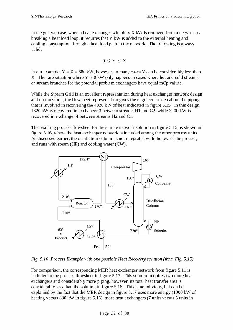
While the Stream Grid is an excellent representation during heat exchanger network designand optimization, the flowsheet representation gives the engineer an idea about the pipingthat is involved in recovering the 4820 kW of heat indicated in figure 5.15. In this design,1620 kW is recovered in exchanger 3 between streams H1 and C2, while 3200 kW isrecovered in exchanger 4 between streams H2 and C1.

The resulting process flowsheet for the simple network solution in figure 5.15, is shown infigure 5.16, where the heat exchanger network is included among the other process units.As discussed earlier, the distillation column is not integrated with the rest of the process,and runs with steam (HP) and cooling water (CW).

Product

DistillationColumn

Compressor

210°

160°

130°

220°

160°270°

60°

Feed 50°

210°

Reboiler

Condenser

74.5°

HP

CW

180°

CW

CW

HP

192.4°

Reactor

Fig. 5.16 Process Example with one possible Heat Recovery solution (from Fig. 5.15)

For comparison, the corresponding MER heat exchanger network from figure 5.11 isincluded in the process flowsheet in figure 5.17. This solution requires two more heatexchangers and considerably more piping, however, its total heat transfer area isconsiderably less than the solution in figure 5.16. This is not obvious, but can beexplained by the fact that the MER design in figure 5.17 uses more energy (1000 kW ofheating versus 880 kW in figure 5.16), more heat exchangers (7 units versus 5 units in


Page 33 of 90

figure 5.16), and finally that all exchangers have temperature driving forces that are at least20°C. Figure 5.16 has one heat exchanger with a large duty (3200 kW) and only 10°Ctemperature difference in the hot end. In these arguments, the distillation column and itsuse of HP steam and cooling water is not included, since the column is operated in thesame way in figures 5.16 and 5.17.

Product

DistillationColumn

Compressor

210°

160°

130°

220°

160°270°

60°

Feed

50°

210°

Reboiler

Condenser

80°

HP

CW

180°CW

CW

HP

190°

Reactor

235.6°

180°

160°

177.6°

Fig. 5.17 Process Example with a maximum Heat Recovery solution (from Fig. 5.11)

In summary, this section has indicated how network optimization can be carried out as adesign evolution, without large modifications to the basic network structure. This methodrequires a good initial design, as the ones that can be established by the Pinch DesignMethod. In practice, cost information is required to actually optimize the network, but thebasic strategy outlined here is still valid:

a) Identify a good starting value for ∆Tmin by pre-optimization based on individualtargets for Energy, Area and Units (also referred to as SuperTargeting).

b) Design an MER network using the Pinch Design Method (section 5.3).

c) Remove the smallest unit by breaking a Heat Load Loop.

d) Restore driving forces by manipulating a Heat Load Path.

One of the major limitations in chapter 5 is the assumption of a global value of ∆Tmin forall process streams and heat exchangers. In industrial applications, differences in heattransfer coefficients must be accounted for in Targeting, Design and Optimization.Another limitation is the fact that sequential procedures as the one outlined here haveproblems handling complicated multiple trade-offs and so-called topology traps asexplained by Gundersen et al., 1990 and 1991.


Page 34 of 90

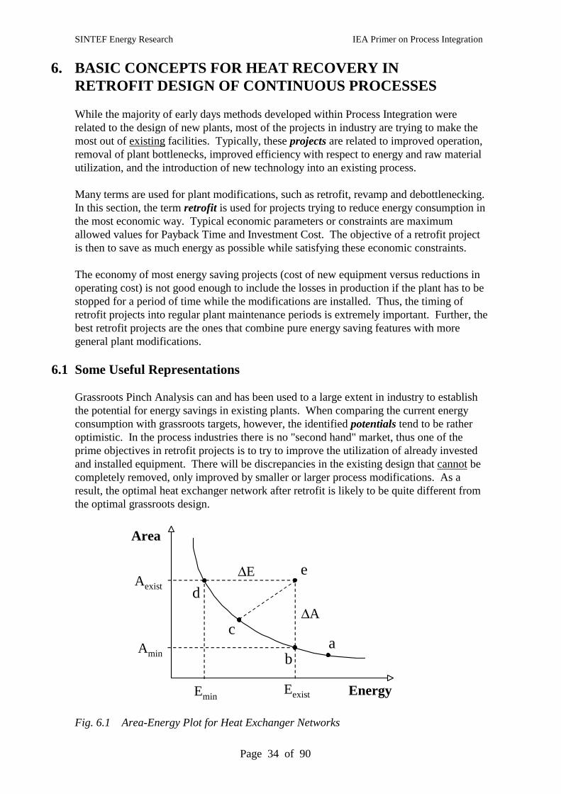
6. BASIC CONCEPTS FOR HEAT RECOVERY INRETROFIT DESIGN OF CONTINUOUS PROCESSES

While the majority of early days methods developed within Process Integration wererelated to the design of new plants, most of the projects in industry are trying to make themost out of existing facilities. Typically, these projects are related to improved operation,removal of plant bottlenecks, improved efficiency with respect to energy and raw materialutilization, and the introduction of new technology into an existing process.

Many terms are used for plant modifications, such as retrofit, revamp and debottlenecking.In this section, the term retrofit is used for projects trying to reduce energy consumption inthe most economic way. Typical economic parameters or constraints are maximumallowed values for Payback Time and Investment Cost. The objective of a retrofit projectis then to save as much energy as possible while satisfying these economic constraints.

The economy of most energy saving projects (cost of new equipment versus reductions inoperating cost) is not good enough to include the losses in production if the plant has to bestopped for a period of time while the modifications are installed. Thus, the timing ofretrofit projects into regular plant maintenance periods is extremely important. Further, thebest retrofit projects are the ones that combine pure energy saving features with moregeneral plant modifications.

6.1 Some Useful Representations

Grassroots Pinch Analysis can and has been used to a large extent in industry to establishthe potential for energy savings in existing plants. When comparing the current energyconsumption with grassroots targets, however, the identified potentials tend to be ratheroptimistic. In the process industries there is no "second hand" market, thus one of theprime objectives in retrofit projects is to try to improve the utilization of already investedand installed equipment. There will be discrepancies in the existing design that cannot becompletely removed, only improved by smaller or larger process modifications. As aresult, the optimal heat exchanger network after retrofit is likely to be quite different fromthe optimal grassroots design.

Fig. 6.1 Area-Energy Plot for Heat Exchanger Networks

Area

Energy

Aexist

Eexist

∆A

∆E

ab

c

d

e

Emin

Amin


Page 35 of 90

In an existing plant, the heat recovery system can suffer from two types of errors, asillustrated in figure 6.1. Each point on the curved line indicates the minimum amount ofheat transfer area that is required to have a certain energy consumption (or level of heatrecovery). Similarly, the curve also indicates minimum energy consumption for a giventotal heat transfer area. The points (a) to (e) represent different design solutions that willbe discussed in the following.

The curved line in figure 6.1, also referred to as the Area-Energy Plot, is constructed bycalculating minimum target values for energy and area as indicated in section 5.2 fordifferent values of the minimum allowable approach temperature, ∆Tmin. With smallvalues of ∆Tmin, the minimum area target is large, while the energy target is low, andopposite for large values of ∆Tmin.

Assume that design (c) is the optimal grassroots heat exchanger network, with an optimaltrade-off between operating cost and investment cost for the current energy and area prices.Network (a) has been correctly designed in the sense that it uses minimum area to achievea certain level of heat recovery. Most likely, this design has been established by the PinchDesign Method. The trade-off in this design is wrong, however, as it uses more energythan would have been optimal with the “current” prices. In a retrofit project, it will be veryhard and costly to improve this network. Moving along the curve from (a) to (c) wouldmean that a number of heat exchangers would have to be taken out of the network. Whatwould be done in practice is to keep most of the existing exchangers and invest in somenew ones. The corresponding retrofit project would move along a curve above theminimum target line, and this curve would be steeper than the target line.

Next, consider design (e), which is located far above the target line. If this had been asuggested new design, both investment cost (area) and operating cost (energy) could havebeen reduced as indicated by ∆A and ∆E. If this is an existing network, however, it is noteconomically tractable to try to reach design (c), since that would involve throwing away alarge number of invested heat exchangers. Again, the retrofit project would follow a curveto the left, but in this case it would be flat in the beginning, since the existing network hasmajor errors that can be corrected by moderate investments, such as re-piping and theaddition of strategically placed new heat exchangers. After correcting the most obviouserrors in the existing design, the cost of recovering additional heat will gradually becomemore costly. This means that the retrofit curve would become steeper, and payback timetherefore increases with the amount of energy saved.

While network (a) is a "good" design (unfortunately with a wrong trade-off), network (e) isa "poor" design, since it uses much more energy than what could have been achieved withthe amount of invested heat transfer area. The errors in design (e) are important in retrofitprojects and will be discussed in detail in this section.

It should also be mentioned that the minimum area figures used to establish the targetcurve in figure 6.1 actually require a large number of heat exchangers, splitters and mixers(referred to as the Spaghetti Design in section 5.2.4). Thus, one would never design on thetarget line, but some small distance above. Figure 6.1 is a quantitative tool to identify thepotential for improved heat recovery, and at the same time a qualitative picture of thesituation indicating how costly the corresponding retrofit projects will be. What areneeded next are some guidelines on how to actually modify the network.


Page 36 of 90

The reason why an existing design, such as network (e) in figure 6.1, is using more thanthe minimum amount of energy (both heating and cooling), is the fact that heat is beingtransferred across the heat recovery Pinch. Such heat transfer can take three differentforms, as indicated in figure 6.2.

The heat recovery Pinch divides the process into a heat deficit part above Pinch and a heatsurplus part below Pinch. Of course, it would not make sense to transfer heat from thedeficit part to the surplus part. Nevertheless, when heat exchanger networks are designedwithout the knowledge about the heat recovery Pinch, such heat transfer is often inevitable.This is why large potentials for energy savings have been identified in existing plants, andthe more complex these processes are, the more likely it is that considerable cross Pinchheat transfer takes place. Typical examples are petrochemical plants and oil refineries,however, significant potentials have also been identified in other industries as well.

Pinch

T

Hot Streams

Cold Streams

ST

Hot Streams

Cold StreamsCW

QPP QPH

QPC

Fig. 6.2 The Penalty Heat Flow Diagram for Heat Exchanger Networks

There may also be practical reasons for such heat transfer across the Pinch. One of themajor limitations of the Composite Curves and the corresponding Pinch Analysis, is thathot and cold streams are regarded to be heating and cooling resources that can be usedwithout limitation. In practice, however, there will be match combinations among hot andcold streams that one would avoid. Examples include safety considerations, geographicaldistance, start-up considerations, ensuring product purity, etc.

In many of these cases, heat transfer across the Pinch is inevitable, however, there aresome degrees of freedom in how this heat transfer takes place. The Penalty Heat FlowDiagram (Linnhoff and O’Young, 1987) in figure 6.2 shows that heat can be transferredacross the heat recovery Pinch in the following three ways:

• Heat transfer from a hot stream above Pinch to a cold stream below Pinch: QPP

• Heating a cold stream below Pinch with hot utility, such as steam: QPH

• Cooling a hot stream above Pinch with cold utility, such as cooling water: QPC

The total Energy Penalty for heat transfer across the Pinch is then the sum of theseindividual heat flow components:

QP = QPP + QPH + QPC


Page 37 of 90

This penalty is then the difference between the current energy consumption and theminimum energy consumption for a given value of ∆Tmin:

QH,exist = QH,min + QPQC,exist = QC,min + QP

The three components of penalty heat flow (QPP, QPH and QPC) can be considered asvariables that can be used to take advantage of the situation when practical constraintsresult in an energy penalty. When trying to minimize the cost penalty of such constraints,the three variables provide two degrees of freedom. This is obvious from figure 6.2, sincethere are two heat load loops that can be manipulated. The following advantages can betaken from a constrained situation:

• QPP means heat transfer at larger driving forces, thus heat transfer area is reduced.

• QPC can be realized as steam production, if the Pinch temperature is high enough.

• QPH means that a cheaper hot utility with lower temperature can be used.

Since the energy target depends on the chosen value of ∆Tmin, the corresponding potentialfor reduced energy consumption is larger for a smaller value of ∆Tmin. The correspondingretrofit project will, however, also be more complex and costly. While targeting methodsexist for the retrofit case that can identify a proper value for ∆Tmin (will be described later),it is common practice in industry to use a larger value for ∆Tmin in a retrofit situation thanthe corresponding and optimal value of ∆Tmin in a grassroots case.

Pinch180°

C2210° 160°

C1210° 50°

H2

220° 60°

H1

270° 160°

160°

Ca

2

2

H

1

1

1000 kW

2500 kW

Cb

980 kW

1320 kW

2200 kW

160°

214.4°

120°

mCp(kW/°C)

18.0

22.0

20.0

50.0

Fig. 6.3 Cross Pinch Heat Transfer in a Stream Grid

Having explained the features of an existing design that is responsible for a larger thanminimum energy consumption, the next logical step is to look at the actual heat exchangernetwork to identify which process/process heat exchangers, external heaters and coolersthat are actually transferring heat across pinch. The Stream Grid is an excellent tool forthis purpose. In figure 6.3, an existing heat exchanger network is drawn in a stream grid insuch a way that the relative position (in temperature) to the Pinch is indicated for all units.


Page 38 of 90

6.2 A Preliminary Retrofit Discussion

It is now easy to identify which heat exchangers that transfer heat across the Pinch, andwhat amount of heat that is transferred across Pinch in each of these units. The sum of allthese cross Pinch occurrences should add up to the total energy penalty. It should benoted, however, that there sometimes are cases where a heat exchanger operating withsmall temperature driving forces is transferring heat from below to above Pinch. Theseheat flows must then be subtracted when calculating the total energy penalty.

The heat exchanger network in figure 6.3 uses 2500 kW of hot utility and 2300 kW of coldutility. The corresponding minimum target values for ∆Tmin = 20°C are QH,min = 1000 kWand QC,min = 800 kW (see the small example used for illustration in section 5.2). The totalenergy penalty for this existing design is thus:

QP = QH,exist - QH,min = QC,exist - QC,min = 1500 kW

For the network in figure 6.3, cross Pinch heat transfer can be identified in heat exchanger(2) and cooler (Ca). The actual amount of heat transfer across the Pinch in these units canbe calculated as follows:

Exchanger (2): QPP = 22 · (220 - 180) = 880 kWCooler (Ca): QPC = 18 · (214.4 - 180) = 620 kW

In this case, there is no external heating below Pinch, and the total energy penalty can becalculated from the occurrences of cross Pinch heat transfer:

QP = QPP + QPH + QPC = 880 + 620 + 0 = 1500 kW

Fig. 6.4 A Retrofit Solution reaching Minimum Energy Consumption

Obvious retrofit projects should involve attempts to reduce heat transfer across the Pinch.Hot stream H2 is a heating resource above Pinch that could be used to heat up cold streamC2 and thus reduce the use of steam in the heater (H). Hot stream H1 is also a heatingresource above Pinch, where some heat in the existing design is lost to cooling water.

3

Pinch180°

C2210° 160°

C1210° 50°

H2

220° 60°

H1

270° 160°

160°

Ca

2

2

H

4

43

1

1

190° 177.6°

1000 kW

1000 kW 620 kW 880 kW

Cb

360 kW

440 kW

2200 kW

160°

180°

180°

80°

235.6°

mCp(kW/°C)

18.0

22.0

20.0

50.0


Page 39 of 90

Trying to realize the total potential for energy savings (1500 kW), would involve two newheat exchangers (3 and 4) and additional area in the existing ones (1 and 2), due to reduceddriving forces. The corresponding heat exchanger network shown in figure 6.4 is actuallyidentical to the initial MER design for the grassroots case shown in figure 5.11. Withoutactually performing cost calculations, it is obvious that the retrofitted network in figure 6.4will be very expensive. It is almost an entirely new heat exchanger network.

An alternative solution would be to try to recover some of the heat that is lost from hotstream H1 into cooling water, by adding a new unit between hot stream H1 and coldstream C2. In this case, the existing heat exchangers are not modified (no additional areais needed), and the simple question is whether the saving of 620 kW of steam and coolingwater will justify the investment in a new heat exchanger (3). The corresponding networkis shown in figure 6.5.

Pinch180°

C2210° 160°

C1210° 50°

H2

220° 60°

H1

270° 160°

160°

Ca

2

2

H

1

1

1000 kW

1880 kW

Cb

360 kW

1320 kW

2200 kW

160°

214.4°

120°

mCp(kW/°C)

18.0

22.0

20.0

50.03

3

620 kW

180°

172.4°

Fig. 6.5 A cheaper Retrofit Solution recovering part of the Potential Energy Savings

Having shown some of the useful representations and indicated a possible "thinking" inretrofit situations based on cross Pinch heat transfer, the remaining part of chapter 6 will bedevoted to a presentation of the methods that can be used for heat exchanger networkretrofit. Similar to the grassroots case, there are four distinct phases also for retrofitdesign:

1) Data Extraction 2) Targeting 3) Design 4) Optimization

There will, however, be significant differences in all of these phases when compared to thegrassroots situation. These differences and the new objectives will be highlighted in thedescription of each of these phases.


While there are a number of similarities between data extraction in the retrofit situationand the grassroots case as described in section 5.1, there are also significant differencesthat will be highlighted here. In both cases, data extraction is a time consuming andcritical activity for the outcome of a Process Integration project.


Page 40 of 90

Typically, for a new design there will be material and energy balances available eithermanually derived or based on a simulation model. A rigorous simulation model has thedistinct advantage that stream data can be extracted directly and even automatically withtoday’s software. Unfortunately, such models may not always be available for an existingplant. In general, the following are possible sources for data that are needed in a retrofitheat recovery project, and often these sources have to be used in combination:

• Measurements (that are often not complete and not reliable)• Design data (that are often outdated after plant modifications)• Simulation models (that may not always reflect true plant behavior)

As a result, data reconciliation is important in retrofit projects. If measurements indicatethat heat extracted from a hot stream in an existing heat exchanger does not match the heatabsorbed by the cold stream in the same exchanger, it is necessary to analyze the situation.Stream data must be modified in such a way that heat balance is obtained; otherwise theheat recovery project will produce unrealistic results. It is important to notice that dataaccuracy is most important in the near Pinch region of the plant. Thus, it is commonpractice to try to establish a first draft of the Composite Curves, and then try to improvethe accuracy only for process streams in the near Pinch region.

Another typical retrofit issue is related to which streams to include in the analysis. Theremay be a number of practical considerations suggesting that certain streams should not beincluded, since heat integration of these streams could cause operational problems. It is,however, good practice to start by including all streams that need heating or cooling, andthen later exclude these streams one by one from the analysis. In this way, the engineerwill know the loss in heat recovery potential from excluding certain streams.

In retrofit projects it is not necessary to iterate between data extraction and targeting, sincethe basic process (reactors, separators) is given and cannot easily be modified for improvedheat recovery potential as the case is for grassroots projects. It would also be expensive tomodify these process units, and would seldom “pay off” in pure energy based projects.

6.4 Retrofit Targets (Phase 2)

Targeting in the Retrofit situation is far more difficult than for Grassroots design. This isso because a number of different changes can be made to the heat exchanger network inorder to reduce energy consumption. Typically, these modifications include:

• Addition of a new heat exchanger• Additional area to an existing unit (for example a new shell)• Change internals in heat exchangers• Modify piping on one side of the exchanger• Modify piping on both sides of the exchanger• Moving a heat exchanger to a new location

Most of these retrofit actions will change the operating conditions for many of the heatexchangers, and a rigorous rating exercise is required to evaluate whether an existing unitwill be able to operate in the new situation. The cost function for the retrofit project willexhibit a discontinuity whenever a heat exchanger switches from being large enough tobecome too small for the new operation.


Page 41 of 90

In other words, the targeting of capital investment (new heat transfer area and new units) ismuch more difficult than in the grassroots case. Energy consumption, on the other hand, ismuch easier to predict, however, knowing the savings in energy cost is of limited value if itis not correctly linked with its corresponding investment cost. That is the true challenge inretrofit targeting.

6.4.1 Different ∆T Representations

The ultimate goal of the targeting exercise is to establish a good starting value for the levelof heat recovery. In grassroots heat exchanger network design (Chapter 5), the parameter∆Tmin (minimum approach temperature) was used to represent this level of heat recovery.In most industrial processes, it does not make sense to require that all heat exchangers (andthus all process streams and utilities) obey the same minimum value for driving forces,since streams (and utilities) in general have very different heat transfer coefficients. Quiteoften, the difference in film heat transfer coefficients can be two orders of magnitude.Thus, some heat exchangers require large ∆T-values in order to avoid excessive heattransfer area, while other units manage well with much smaller ∆T-values.

Since this document is a Primer with focus on the key concepts in Process Integration, wedid not discuss the details about heat transfer conditions and driving forces in Chapter 5.When considering the retrofit case, however, there are many reasons why we need toreconsider this question. Without going into too many details, we should at leastacknowledge the need for two different approach temperatures:

HRAT = Heat Recovery Approach TemperatureEMAT = Exchanger Minimum Approach Temperature

While HRAT, as the name indicates, is a key parameter for the level of heat recovery (it issimply defined as the smallest vertical distance between the Composite Curves), EMAT isthe minimum allowable temperature difference for the individual heat exchangers. Inorder to reach a certain level of heat recovery, (as specified by HRAT), the followinginequality must be satisfied:

0 ≤ EMAT ≤ HRAT

As mentioned in section 5.2, it is also possible to assign individual contributions to theminimum driving forces for each stream and utility. Typically, these ∆T contributionsshould reflect heat transfer conditions, but they can also be used to represent the need forexpensive material of construction, expensive heat exchanger types, etc. In this case,EMAT becomes stream dependent, and the following must be satisfied for a matchbetween hot stream/utility (i) and cold stream/utility (j):

∆Ti,j ≥ EMAT (i,j) = ∆Ti + ∆Tj

where ∆Ti and ∆Tj are the individual stream contributions. To illustrate how thesedifferent ∆T-values apply in retrofit situations, consider a typical oil refinery with a crudepreheat train that warms up the crude from ambient temperature to the inlet of the furnacejust before the crude fractionation tower. This is a complex heat exchanger network withmany units, a large number of stream splits and considerable heat recovery from various


Page 42 of 90

hot streams in the refinery. In retrofit projects for such plants, it is common to design for alevel of heat recovery that corresponds to HRAT = 30°C, however, the actual energyconsumption in many such crude preheat trains corresponds to a value of HRAT wellabove 50°C. At the same time, there will be some heat exchangers typically where ∆T inone end of the units is in the range between 10 and 15°C. Thus, EMAT and the individualcontributions ∆Ti and ∆Tj are considerably less than HRAT.

6.4.2 A Simple Energy Target

An obvious way to establish a target for energy savings in a retrofit project is to calculatethe minimum external heating requirements for different values of HRAT (previouslyreferred to as ∆Tmin). One of these values of HRAT (typically a large one) corresponds tothe current energy consumption, and the targeting exercise then becomes the identificationof a new value of HRAT that is less than the “existing” value of HRAT:

HRATnew ≤ HRATexisting

By plotting minimum energy consumption (or minimum energy cost in the case of multipleutilities) as a function of HRAT, it is possible to identify potential starting values of HRATfor the retrofit project.

Fig. 6.6 A typical Energy Target Plot for the Retrofit Case

Consider the Energy Target Plot in figure 6.6, where the change in the slope illustrates thetypical situation that minimum energy consumption does not always increase directlyproportional with minimum driving forces. As a result, there are certain levels of heatrecovery (represented by HRAT) that are more likely to be good retrofit candidates thanothers. Consider point (a) in figure 6.6. When trying to move towards larger energysavings, the change in QH,min is relatively small, while the reduction in HRAT isconsiderable. Normally, this means large investments with moderate savings.

Figure 6.6 also indicates how the targeted savings in energy consumption (∆E) can be readfrom the diagram for different values of HRAT. Also, by looking at figure 6.6, one mayconclude that point (a) seems to save too little energy, while point (c) involves too largeinvestments. Qualitatively, it may look as if point (b) provides a good trade-off between

HRAT

QH,min

QH,exist

QH,new

HRATnew HRATexist

∆E a

b

c


Page 43 of 90

investments and savings in the retrofit case; thus HRATnew is a good starting value for theretrofit project. Cross Pinch Analysis (section 6.1 and figure 6.3) will then be performed,where the existing heat exchanger network is drawn in a stream grid with a Pinch pointaccording to ∆Tmin = HRATnew.

6.4.3 Targets for Area and Investment Cost

As stated in the beginning of section 6.4, targeting for heat transfer area and investmentcost is far more complicated and uncertain in the retrofit situation than in the grassrootscase. The identification of “promising” starting points in figure 6.6 may work in somecases, however, there is a need to quantify not only the energy saving part, but also theinvestment in new equipment and changes in piping.

Within Pinch Analysis, a Retrofit Targeting procedure has been proposed that is based onthe concept of Area Efficiency (Tjoe and Linnhoff, 1986). This parameter can be easilyobtained from the existing design and can be mathematically formulated as:

α = [ Amin ] / [ Aexist ]

where α = Area EfficiencyAmin = Minimum area for the current level of heat recovery (HRATexist)Aexist = Total heat transfer area in the existing network

A conservative assumption is that any new invested heat transfer area will at least have thesame utilization level (area efficiency) as the installed area. This assumption (also referredto as the “constant α” approach) proved to work nicely for oil refineries and crude preheattrains, where area efficiency in existing plants was quite high (above 80%), while it did notwork equally well in other industries. In processes with less heat integration, the constantα assumption can be too conservative. Attempts have been made to overcome thisproblem; one is the so-called “incremental α” approach (Silangwa, 1986), which meansthat area efficiency will change (improve) during the retrofit project.

Fig. 6.7 A typical Retrofit Target Plot for Savings and Investment Cost

Investment(US$)

Savings(US$/yr)

Invmax

a

bdc

PB=1PB=2

PB=3


Page 44 of 90

Irrespective of the actual approach chosen, using some kind of assumptions about areaefficiency for new heat exchangers or additional shells, it becomes possible to estimate theneed for new area (and thus investment cost) when targeting for different values of HRAT.By combining target values for area and energy for different values of HRAT (starting withthe existing HRAT and then decreasing this value gradually), the Retrofit Target Curve infigure 6.7 can be obtained.

The curved line in figure 6.7 shows corresponding values for annual savings in energy costand the total investment for new equipment (including installation). Each point on thecurve represents a certain level of heat recovery (HRAT), starting in the origin of thediagram, where there are no investments made and no savings earned. Thus, the originrepresents the situation before the retrofit project is started, and moving along the curve tothe right means heading for smaller HRAT values and higher levels of heat recovery. Asdiscussed in section 6.1, the most obvious errors in the existing network can be correctedfirst, often with small or moderate investments. Thus, the target line is initially steep, butthen becomes more flat as we move towards higher levels of heat recovery.

Payback Time is simply defined as the Investment Cost divided with the Annual Savingsin Operating Cost (energy). Considering the nature of the target curve in figure 6.7, it isobvious that Payback Time increases as we move along the curve towards larger energysavings. The dashed lines in the diagram illustrates typically Payback Times (PB) of one,two and three years. It is also quite common that management has set an upper limit on theinvestment that will be put into a certain energy saving project (indicated as Invmax infigure 6.7). There will also be constraints on the Payback Time, and depending on whethermaximum Payback Time for this particular example is set to two or three years, the retrofittargeting exercise will identify points (b) if minimum payback is two years or point (c)limited by maximum investment, if maximum payback is three years.

Points (b) and (c) in figure 6.7 correspond to different values of HRAT, which means thata target for the level of heat recovery has been identified. This target is an improvementcompared with the more simplified discussion in section 6.4.2, since investment cost hasbeen included and quantified, even though there are large uncertainties in these numbers.Again, once the new value for HRAT has been identified, the next stage is a cross Pinchanalysis, as described in section 6.1.

6.5 Retrofit Design (Phase 3)

The Cross Pinch Analysis mentioned in the previous section is a good starting point for thedesign exercise. The first methods suggested to remove heat exchangers that transferredheat across the Pinch and to try to reuse these units in new locations. Since, however, heatexchangers in most cases are tailor made for a certain application (flowrates and types ofstreams) it is not easy and quite expensive to follow this approach.

6.5.1 Temperature “Shifting” of Heat Exchangers

Instead, Tjoe and Linnhoff, 1986, suggested to “shift” heat exchangers away from a crossPinch situation. This shifting involves changes in operating conditions for the unit in sucha way that hot stream temperatures are reduced and/or cold stream temperatures increased.The result is that cross Pinch heat transfer in that particular unit is reduced and possiblyeliminated. Heating resources are released above Pinch and or cooling resources are


Page 45 of 90

released below Pinch. Consider the existing heat exchanger network in figure 6.3 that wasused in the preliminary retrofit discussion of this chapter.

The cooler Ca and heat exchanger (2) are transferring a total of 1500 kW across Pinch,which is why external heating (2500 kW) and cooling (2300 kW) requirements are largerthan the established minimum figures (1000 kW of heating and 800 kW of cooling). Theshifting procedure means that the inlet temperature of stream H1 to the cooler Ca shouldbe reduced from 214.4°C to at least 180°C (Pinch temperature for hot streams). This willrelease a heating resource from stream H1 above Pinch equal to 620 kW, and the duty ofcooler Ca is reduced from 980 kW to 360 kW.

Similarly, the inlet temperature of stream H2 to heat exchanger (2) should be reduced from220°C to 180°C. Assuming that the duty of this unit remains unchanged at 2200 kW(should always be questioned during network optimization), the duty of cooler Cb will bereduced by 880 kW to 440 kW. Figure 6.8 shows the incomplete network after theseshifting operations. As indicated by the rectangles, there are two heating resources thathave been released and not yet utilized above Pinch.

Fig. 6.8 Incomplete Heat Exchanger Network after “Shifting”

6.5.2 Introduction of New Heat Exchangers

The next obvious question is how to utilize these new heating resources above Pinch.Since cold stream C1 already is fully covered through heat recovery from hot stream H1,the obvious option is to try to use heat from hot streams H1 and H2 to partially heat coldstream C2 in order to reduce steam consumption in the heater.

Following the basic philosophy of the Pinch Design Method, cold stream C2 cannot fullyutilize the two new heating resources (would involve taking both streams H1 and H2 downto Pinch temperature) unless stream C2 is split into two branches. Since mCp for streamC2 (50 kW/°C) is larger than the sum of mCp (18+22 kW/°C) for streams H1 and H2, thisis a feasible option. Alternatively, the heating resource related to hot stream H1 could beshifted to the beginning (hottest part) of the stream. This option has already been shown infigure 6.4, however, as indicated in the same figure, heat exchanger (1) has considerablyreduced driving forces and additional area is inevitable.

Pinch180°

C2210° 160°

C1

210° 50°

H2

220°60°

H1

270° 160°

160°

Ca

2

2

H

1

1

1000 kW

2500 kW

Cb

360 kW

440 kW

2200 kW

160°

214.4°

80°

mCp(kW/°C)

18.0

22.0

20.0

50.0

180°

620 kW

880 kW

180°


Page 46 of 90

Figure 6.9 shows the initial retrofitted heat exchanger network when the stream splitoption is chosen. In this case, the operating conditions (duty and temperatures) for heatexchanger (1) is unchanged, and no additional area is needed. Heat exchanger (2) has,however, reduced driving forces with the same duty, and additional area is needed asindicated. A comparison with the alternative retrofit design in figure 6.4 will be madebefore going into the optimization stage.

Fig. 6.9 Complete Retrofitted Heat Exchanger Network with Stream Split

In order to compare the two alternative initial retrofit heat exchanger networks in figure 6.4and figure 6.9, details about heat transfer conditions and cost equations are needed. In thisparticular case, we do have information about heat transfer coefficients for streams andutilities (table 5.1), however, for the purpose of this Primer we do not want to go intodetailed cost calculations. Instead, comparison between the two alternatives will be madeon the basis of a simple UA analysis.

It is easy from the heat transfer equation to calculate UA-values for the heat exchangersbefore and after retrofit modifications. If we assume that the units are pure countercurrent, UA-values can be obtained from:

UA = Q / ∆TLM

Table 6.1 shows UA-values for existing and new heat exchangers before and after retrofitmodifications for the two alternative designs A (figure 6.4) and B (figure 6.9). Utilityexchangers are not included, since the duty of these units are reduced in such a way that noadditional area is needed (actually, these units will not be fully utilized after the retrofitmodifications). Isothermal mixing is assumed for stream C2 after the split.

As indicated in table 6.1, the UA analysis does not give any strong preference for design A(figure 6.4) or design B (figure 6.9). The difference in total UA needed in the retrofittednetworks is not significant, and a stronger argument for choosing design B is probably thatthe number of modifications is less, since there is no change needed for heat exchanger (1)in this case, however, there is a stream split introduced.

Pinch180°

C2210° 160°

C1

210° 50°

H2

220°60°

H1

270° 160°

160°

Ca

2

2

H

1

1

1000 kW

1000 kW

Cb

360 kW

440 kW

2200 kW

160°

214.4°

80°

mCp(kW/°C)

18.0

22.0

20.0

50.0

180°

620 kW

880 kW

180°4

3

4

3

190°


Page 47 of 90

Table 6.1 UA-values (kW/°C) for two alternative Retrofit Designs

Existing Retrofit NetworksHeat Exchanger Design Design A Design B

1 17.49 44.12 17.492 33.91 89.20 89.203 0 9.07 27.994 0 29.52 35.68

Total 51.40 171.91 170.36

While both design A and design B fully recover the energy saving potential of 1500 kW, inmost cases one can only justify economically to realize some fraction of this potential. Thefigures for UA listed in table 6.1 indicate that heat transfer area must be more than tripledin order to reduce energy consumption to its minimum for HRAT = 20°C. Thus, morerecent retrofit methods use a “greedy” approach trying to identify the most economicretrofit projects with the fewest number of topological changes.

6.5.3 Matrix Methods for Retrofit Design

Some interesting matrix based methods have also been proposed for heat exchangernetwork retrofit situations. Shokoya, 1992, focused on heat transfer area in a methodwhere targeting and design are closely linked. The so-called Area Matrix method is anadoption of the vertical heat transfer model (see the Area Targeting method in section5.2.4). For various levels of heat recovery, the best vertical match area contribution isfound using Linear Programming (LP). The result is a significantly improved retrofit areatargeting method when compared with the constant α or incremental α methods mentionedin section 6.4.3. While the Area Matrix method primarily is a targeting procedure, theresults from the LP optimization can also be used for retrofit design.

Another matrix based method for retrofit design is the Cost Matrix method developed byCarlsson et al., 1993. The method is based on the experience from a number of retrofitprojects that other costs such as pumping and piping may have a larger influence on theoptimal design than the number of units and heat transfer area. A Cost Matrix for possiblematches is established, where the cost for each match is estimated taking into accountparameters such as physical distance between process streams, material requirements, typeof heat exchangers, auxiliary equipment (such as valves), heat transfer coefficients, spacerequirements, pumping cost, maintenance cost and fouling. The method uses the greedyapproach due to its sequential nature, and there is no targeting involved.

6.5.4 More Recent Retrofit Methods

A number of more recent methods for retrofit heat exchanger networks using optimization(Mathematical Programming) to a large extent have been developed (e.g. Asante and Zhu,1996, Briones and Kokossis, 1996). Due to the rather complex nature of these methods,however, they are only briefly mentioned in chapter 9 and omitted here. The complexity ofthese methods also means that software is an absolute requirement. Typically, thesemethods acknowledge the fact that only a few carefully selected modifications will beeconomically worthwhile, and the approach is to identify these retrofit actions.


Page 48 of 90


As mentioned in the previous section, optimization is used in some of the more recentretrofit methods for network design, and the distinct classification into targeting, designand optimization has been reduced and almost eliminated. This section, however, willdiscuss how initial retrofit designs developed using the methods described in sections 6.5.1and 6.5.2 can be improved economically and simplified with respect to network structure,using the same optimization philosophy as in the grassroots case.

Degrees of freedom in the form of heat load loops and paths as well as stream splits canbe used to improve the initial retrofit design. One important new aspect in the retrofit caseis to maximize the utilization of existing heat exchangers. After the shifting of cross Pinchheat exchangers and the introduction of new units, some of the existing heat exchangersmay have a reduced duty and therefore no longer require all the area installed. In suchcases it may be worthwhile to shift duty in heat load loops and/or paths until the existingunits are better utilized.

Similar to grassroots situations, retrofit network optimization is a combination of discreteand continuous adjustments. The discrete part takes care of the removal of small new heatexchangers or small area additions to existing units, while the continuous part takes care ofthe trade-off between investment cost and obtained energy savings. The continuous partalso includes, as mentioned above, the maximum utilization (if possible) of existing units.

Figure 6.5 shows an alternative retrofit heat exchanger network for the example problem,where only one topological modification is suggested. The introduction of the new heatexchanger (3) between H1 and C2 recovers heat that is lost to cooling water above Pinch inthe existing design. In this retrofit alternative, the existing heat exchangers (1) and (2) arenot changed, and the optimization simply becomes a one-dimensional search to identify thelargest duty for heat exchanger (3) that satisfies constraints such as maximum PaybackTime and maximum Investment Cost. Figure 6.10 illustrates that the optimization problemis reduced to the issue of finding the best duty for the new heat exchanger (variable y maytake positive and negative values), and how this affects the heat load path from the heaterthrough the new unit to the cooler Ca. Temperatures T1 and T2 depends on the value of y.

Fig. 6.10 A limited Retrofit Network Optimization Problem

C2210° 160°

C1

210° 50°

H2

220°60°

H1

270° 160°Ca

2

2

H

1

1

1880+y

Cb

360+y

214.4°

mCp(kW/°C)

18.0

22.0

20.0

50.0

T1

620-y

3

3

T2


Page 49 of 90

7. BASIC CONCEPTS FOR HEAT RECOVERYIN BATCH PROCESSES

Batch processes have several advantages compared with continuous processes. Whilecontinuous processes are "tailor-made" to serve basically one major purpose for 15-20years, batch processes typically consist of more general-purpose equipment, which makessuch plants far more flexible. This becomes increasingly important in a world of highvalue products with shorter lifetime.

By its very nature, however, batch processes cannot reach the same degree of utilization ofthe equipment as continuous processes. Typically, time is lost in a number of operationssuch as feeding, unloading, cleaning, etc. Time analysis of the operation of such plants(also called scheduling) is therefore extremely important. The time aspect is also a keyfactor when studying heat recovery of such processes.

7.1 Introduction

In order to maximize the use of invested equipment, Gantt Diagrams are heavily used inbatch industries. In these diagrams, both the duration of each operation and the relativesequence of operations depending on each other, can be plotted as function of time. Sinceefficient schedules are important, there is a very strong link between design, scheduling(short term) and planning (long term) of such processes.

This section will primarily concentrate on the use of Pinch Analysis based methods for theidentification of Heat Recovery opportunities. While energy cost is small compared withthe cost of equipment and raw material for a majority of batch processes, it has been shownin some cases that the energy system may be responsible for bottlenecks in the plants. Oneshould also mention the more general spin-off from Systems oriented studies such as PinchAnalysis, that more insight about the various aspects of the process is obtained. Also,there are quite a few batch industries where energy cost is considerable, and whereimproved energy efficiency may give the company a competitive edge.

7.2 Heat Recovery and Design Phases

There are several differences between batch and continuous processes when studying heatrecovery. The most important difference is the time aspect in batch processes where acertain amount of heat is available between specified temperatures, and also betweenspecified times. Thermal energy in such plants has two qualities, temperature and time.

While most plants are operated with repeated cycles, some of the material in this sectionrelates to a single batch only, however, the effect of cyclic operation will be addressed.When plants are operated in a cyclic manner, the question about "before" or "after"becomes more vague than the situation when considering a single batch.

It should also be mentioned that the majority of the literature covering design, scheduling,planning and heat integration of batch processes assumes that these plants are operatedwith a rigid schedule. Some plants do not operate according to a predefined schedule, andquite often the schedule is somewhat uncertain due to upsets in plant operation. Delaysmay then destroy the nice schedule that was planned.


Page 50 of 90

Heat exchange between process streams in batch processes can take place in two differentways:

• Direct using a Heat Exchanger if the streams exist in the same time period • Indirect using a Heat Storage System if the streams do not co-exist in time

When heat storage is expensive, an alternative solution would be to consider reschedulingin such a way that direct heat exchange becomes possible.

When using Pinch Analysis for heat recovery in batch processes, the Design Stages aresimilar to the case with continuous processes, however, the actual content of each phasecan be quite different. The following four phases should be carried out in sequence:

1) Data Extraction (collecting data for the process and the utility system)2) Targeting (identify maximum heat recovery using direct/indirect heat transfer)3) Design (establish an initial network of heat exchangers and heat storages)4) Optimization (improve the initial network using degrees of freedom)

First, however, it is important to make sure that a proper problem definition has beenestablished. This also includes relevant cost data and economic criteria. It is alsoimportant to identify the actual schedule, and to what extent the schedule is fixed.


In section 5.1 it was mentioned that the most time consuming and often most critical phaseof heat recovery projects, is the collection and evaluation of process data to be used in theanalysis and design. In batch processes, data extraction is even more complicated. Inparticular, there are two new problems to deal with in batch processes. The first is theobvious time aspect, and the second is the fact that several types of streams exist.

A central part of data extraction is the identification of heating and cooling requirements inthe process. The necessary data for each process stream are the following:

m = mass flowrate (kg/s, tons/h, etc.)Cp = specific heat capacity (kJ/kg°C)Ts , Tt = supply and target temperature (°C)ts , tf = start and finish time (s, h, etc.)∆Hvap = heat of vaporization for streams with a phase change (kJ/kg)

In order to analyze heat transfer area and investment cost for heat exchangers or heatstorage systems, film heat transfer coefficients (h) are needed. In continuous processes, theheat flow (often referred to as heat duty) of a hot stream can be calculated by (index C forcontinuous):

QC = m • Cp • (Ts - Tt ) (kW)

In batch processes, the total amount of heat is a more representative property, and can becalculated for a hot stream by (index B for batch):

QB = m • Cp • (Ts - Tt ) • (tf - ts ) (kWh)


Page 51 of 90

Based on the start and finish times of each stream exchanging heat, a Gantt Diagram thatonly relates to heat recovery can be constructed.

During data extraction the following four types of streams can be encountered:

1) Streams with fixed or constant Ts, Tt, ts, tf, and Q. This corresponds to the situation incontinuous processes apart from the time aspect.

2) Streams with a gradual change of Q with time, even though temperature is constant.This can be the case when a volatile component is vaporizing from a batch reactor.

3) Streams with a gradual change in temperature with time, even though Q is constant.This can be the case when a liquid tank is heated with electric coils.

4) Streams with a gradual change in both Q and temperature with time. This can be thecase when a batch reactor is heated or cooled with steam or cooling water. Duringheat exchange, the temperature driving forces are reduced, resulting in a reduced Q.

7.4 Energy Targeting (Phase 2)

A number of different methods exist for identifying minimum energy consumption inbatch processes. Many of these methods are inspired by Pinch Analysis originallydeveloped for continuous processes. Various assumptions are used, and as a result,different target values are obtained providing the engineer with valuable information.Thus, it is difficult to claim that any of these methods are better than the others, they justserve different purposes. The most important among these assumptions are:

• Whether Heat Storage is used or not. • Type of Heat Storage used and the degree of Temperature Loss. • Selected ∆Tmin value for the Heat Storage • Single Batch or Cyclic Operation

Methods for Energy Targeting in batch processes can be classified in two major groups:

I. Methods where Temperature is considered the Primary Constraint, while Time isconsidered to be a secondary concern, in some cases not included at all:

TAM : Time Average ModelTSM : Time Slice ModelCA : Cascade AnalysisBUC : Batch Utility Curves

II. Methods where Time is considered the Primary Constraint, while Temperature isconsidered to be a secondary concern:

TPA : Time Pinch Analysis

The Time Average Model (Linnhoff et al., 1988), for example, neglects time completelyand assumes that heating or cooling of a stream takes place in the entire batch period. An“average heat duty” obtained from the real heat duty multiplied with the actual time span


Page 52 of 90

for the stream and divided with the total batch period is used in TAM. This may seem togive a target of limited value, but is actually the minimum energy consumption for cyclicbatches and unlimited ideal heat storage. The obtained number can then be used as arigorous lower bound on energy consumption.

Time Pinch Analysis (Wang and Smith, 1995), on the other hand, neglects temperaturefeasibility, which again may seem to give a target of limited value. This method does,however, identify the Time Pinch of the processes, and also suggests what is possiblethrough process modifications, including the use of heat pumps to overcome negativetemperature driving forces.

While TAM and TPA are the extremes, this section attempts to indicate that each methodwill result in different target values for energy consumption, and this will be illustrated bya small and simple example. Table 7.1 shows the process streams for the example. Noutilities are included, however, they are assumed to be available in sufficient amounts andtemperature levels. In the targeting exercise, it is assumed that ∆Tmin = 10°C for bothdirect (heat exchangers) and indirect heat transfer (heat storage systems). In practice, thisis not very realistic, but serves the purpose of illustrating the various targeting methods.

7.4.1 Time Average Model (TAM)

This method has already been discussed above, and the energy targets obtained serve theonly purpose to indicate the absolute maximum heat recovery that can be obtained for acyclic process, when an unlimited number of ideal heat storages (no temperature loss) areallowed. As such, it provides a rigorous lower bound on energy consumption, andindicates the potential for rescheduling or heat storage systems.

The main problem with the TAM method, apart from its extremely optimistic assumptions,is that one cannot distinguish between direct and indirect heat transfer in the target values,which is important information when estimating total cost.

Table 7.1 Stream Data for a small Example

Stream Ts Tt mCp ts tf QC QB

Name (°C) (°C) (kW/°C) (h) (h) (kW) (kWh)

H1 170 60 4.0 0.25 1.00 440 330H2 150 30 3.0 0.30 0.80 360 180C1 20 135 10.0 0.50 0.70 1150 230C2 80 140 8.0 0.00 0.50 480 240

7.4.2 Time Slice Model (TSM)

The next logical step is to split the batch period into smaller Time Intervals (time slices),and consider heat recovery separately in each of these intervals. By increasing the numberof intervals, the target values for minimum external heating and cooling gradually changesfrom the TAM targets to new values for heat recovery that is feasible without heat storage.

An obvious way to identify these time intervals is to use the start and finish times for allprocess streams involved in heating or cooling. The Gantt Diagram in figure 7.1 illustratesthis for the small example in table 7.1.


Page 53 of 90

Stream

0.0 0.25 0.3 0.5 0.7 0.8 1.0Time (h)

H1

H2

C1

C2

Fig. 7.1 Gantt Diagram for Hot and Cold Streams in the small Example

The difference between the TAM and TSM targets indicates the potential for reducingenergy consumption through process modifications such as rescheduling and/or the use ofheat storage, after direct heat exchange has been maximized.

7.4.3 Cascade Analysis (CA)

A more systematic way to consider the time aspect is to use a Two-Dimensional HeatCascade (Kemp and Deakin, 1989), where heat can be transferred to lower temperature(direct heat exchange) or a later time interval (indirect heat exchange using storage).Again, the obvious way to establish this cascade is to use the supply and targettemperatures as well as the start and finish times for all process streams. In some cases,this may give a large number of intervals, however, when the method is implemented intocomputer software, this should not be a major obstacle.

- 10 - 1 - 1 + 7 + 3.5 + 4 + 2.5

- 110 - 11 - 11 - 33 + 38.5 + 44 - 82.5

0 + 4 + 16 + 16 + 8 + 16 + 60

0 + 6 + 42 - 18 + 21 + 24 + 75

0 0 + 18 - 42 + 9 0 - 15

Temp.Interv.

Time Intervals

0-0.25 0.25-0.3 0.3-0.5 0.5-0.7 0.7-0.8 0.8-1.0 Sum165

145

140

85

55

25

Fig. 7.2 Two-Dimensional Heat Cascade for the small Example

Figure 7.2 shows the two-dimensional heat cascade for the small example problem, wherethe 4 process streams result in 5 temperature intervals and 6 time intervals. The last


Page 54 of 90

column takes the heat balance for each temperature interval over all time intervals, thus itshows the overall heat cascade used in the TAM method.

Notice that modified temperatures have been used (average between hot and cold intervaltemperatures) in the same way as for continuous processes. The dotted lines indicate theindividual Pinch points for each time interval. The numbers in the boxes (intervals) areheat balance figures given in kWh, where a positive sign means heat surplus.

Different strategies can be used in the Cascade Analysis (CA). When transferring heatwithin time intervals only, the TSM targets will be obtained, and no heat storage is needed.If heat primarily is transferred within the same temperature interval to later time intervals,heat degradation is minimized, and it may be possible to use a cheaper hot utility at lowertemperature. This strategy will, however, result in a considerable amount of heat beingstored for later use. Alternatively, one could transfer heat from below Pinch in one timeinterval to the region above Pinch in a later time interval.

For small problems, as the one illustrated here, it is possible to carry out the analysis andobtain the targets by studying the two-dimensional heat cascade in figure 7.2. For largerproblems, however, this becomes quite a task. For this reason, graphical diagrams havebeen developed, such as the Heat Recovery Plot. Figure 7.3 shows such a diagram for thetwo neighboring time intervals 3 (0.3 - 0.5 h) and 4 (0.5 - 0.7 h). Time interval 3 has a netheat surplus of 64 kWh, while time interval 4 has a net heat deficit of 70 kWh. If heatfrom time interval 3 is available at a high enough temperature, it should be possible totransfer 64 kWh indirectly from time interval 3 to time interval 4 by using heat storage.Figure 7.3 shows that this indeed is possible, at least in theory (or more correctly: from athermodynamic point of view).

180

140

100

60

20

T (°C)

Q (kWh)

20 40 600

QH,min = 6 kWh

∆Tmin = 10°C

80 100

Qrecov = 64 kWh

Time Interval 3 Time I

nterval 4

Fig. 7.3 Heat Recovery Plot for Time Intervals 3 and 4 for the Example

The Heat Recovery Plot is similar to the Grand Composite Curve, in the sense that heatcascade figures are plotted versus temperature. One time interval is plotted as a heatsource, and the other interval as a heat sink. In figure 7.3, the scope identified for heatrecovery by indirect exchange through a heat storage system, is rather optimistic. If only


Page 55 of 90

latent (constant temperature) heat storages are considered, and indirect heat transfer from ahot stream through storage to a cold stream is allowed at ∆Tmin = 10°C (the same as fordirect heat exchange), an infinite number of storages would result as we approach the heatrecovery pinch for heat transfer between time interval 3 and 4. The situation would besomewhat easier if sensible heat storage systems are assumed.

Nevertheless, the Heat Recovery Plot can be used to find a rigorous upper bound forindirect heat transfer, after direct heat transfer is maximized in each time interval. It is alsopossible to plot more than one time interval as heat source and/or heat sink. The reason forplotting two neighboring time intervals is to reduce time for storage, which affects heatloss in the storage system.

The Heat Recovery Plot can also be used to find the maximum amount of indirect heattransfer through storage when only a limited and specified number of storages is allowed.This is illustrated in figure 7.4, where only one latent heat storage system is allowed, andwhere the total value for ∆Tmin is equally distributed among heat transfer between the hotstream(s) in time interval 3 and the heat storage, and heat transfer between the heat storageand the cold stream(s) in time interval 4. Notice that one of the curves has been inverted inorder to identify the temperature where the heat transferred to the storage from hot streamsequals the heat transferred from the storage to the cold streams.

As shown in figure 7.4, the amount of heat recovered is reduced from 64 kWh for idealand unlimited storage to 43.2 kWh when only one heat storage is allowed. With largervalues for ∆Tmin, the amount of heat recovered would be reduced even further. If two ormore storages are allowed, the graphical procedure becomes more complicated.

180

140

100

60

20

T (°C)

Q (kWh)

20 40 600

∆T = 10°C

80 100

Time Interval 3 Time I

nterval 4

Heat Storage

Qrecov = 43.2 kWh

Fig. 7.4 Heat Recovery Plot for the Example with only one Heat Storage

7.4.4 Batch Utility Curves (BUC)

Another graphical diagram has been developed for the identification of appropriatetemperature levels for heat storages and external utilities. The Batch Utility Curves(Gremouti, 1991) are based on the Grand Composite Curve for each time interval. First,


Page 56 of 90

these Grand Composite Curves are separated into two different curves at the individualPinch temperature for each time interval. The part below Pinch is a Heat Source, while thepart above Pinch is a Heat Sink. Then all existing "pockets" are removed from the curves,and finally the remaining segments are added into Total Heat Source and Sink Profiles.

These curves are similar to the Total Site Source and Sink Profiles for studies of total siteswhere continuous processes exchange heat indirectly through the steam system. In batchprocesses, these so-called Batch Utility Curves (see figure 7.5) are used to considerindirect heat exchange through heat storage systems.

Since the Hot and Cold Utility Curves are monotonic with temperature, the amount of heatthat can be sent to storage from the Heat Source Profile (Cold Utility Curve) is increasingas we move to lower temperatures. The need for such heat in the Heat Sink Profile (HotUtility Curve) is, however, decreasing towards lower temperatures.

By considering the two curves it is quite easy to identify the temperature level for a singleheat storage system. Once the number of heat storages is allowed to be more than one,however, the picture gets more complicated. In addition, the load and level for the variousutilities must also be considered simultaneously with the selection of temperature levelsand amounts of heat for the storage systems.

T (°C)

Q (kWh)

- 200 - 100 1000

180

140

100

60

20

200- 300

ColdUtilityCurve

HotUtilityCurve

Fig. 7.5 Batch Utility Curves for the Example

As always with such graphical diagrams, a major limitation is the fact that the identities ofthe individual streams are lost. For the Heat Recovery Plot in figures 7.3 and 7.4, we needto go behind the curves to identify the actual hot and cold streams that should be linkedwith the heat storage system. In the Batch Utility Curves in figure 7.5, the situation is evenworse, since we also have lost the identities of the various time intervals.

This is a major criticism and disadvantage of almost all graphical diagrams that have beenintroduced within Pinch Analysis. Without information about the number of streamsinvolved as well as their actual identity, it is almost impossible to make any reasonableestimation of the investment cost involved.


Page 57 of 90

7.4.5 Time Pinch Analysis (TPA)

This method will only be briefly described, since neglecting temperature feasibility appearsto be a rather drastic assumption. By plotting heat duties as function of time, two newdiagrams are produced that are similar to the Composite Curves and Grand CompositeCurve for continuous processes. It should also be mentioned that the approach taken inthis method minimizes degradation of heat to lower temperatures.

The TPA Composite Curves can be used to identify bottlenecks for heat recovery in batchprocesses, referred to as the Time Pinch. The TPA Grand Composite Curve can be usedto distinguish indirect heat exchange (storage) from direct heat exchange.

7.4.6 Summary of Methods for Batch Targets

As mentioned earlier, rescheduling is an alternative solution to the use of heat storage,which tends to be quite expensive. Using heat storage, however, adds flexibility to theprocess, and heat recovery becomes less dependent on a fixed schedule. Tools that can beused to consider rescheduling include the Gantt Diagram, the Two-Dimensional HeatCascade and Time Pinch Analysis.

To illustrate the different targets that can be calculated with the various methods discussedin this section, some scenarios are listed in table 7.2. For reference and comparison, totalheating needed by the cold streams is 470 kWh, while total cooling needed by the hotstreams is 510 kWh.

Table 7.2 Various Energy Targets for the small Example (all numbers in kWh)

Method Assumption QH,min QC,min Qstorage

TAM Ideal Storage, Cyclic Operation 20 60 n.a.TSM Maximum Direct, No Storage 198 238 0CA-1 Maximum Direct, No Storage 198 238 0CA-2 Single Batch, Ideal Storage 134 174 64CA-3 Cyclic Operation, Ideal Storage 20 60 178CA-4 Single Batch, Only One Storage 174 214 24

The actual numbers for TAM can be obtained by considering the last column of figure 7.2,where the net heat deficit above Pinch (dotted line) is 20 kWh and the net heat surplusbelow Pinch is 60 kWh. The minimum external heating requirements (QH,min) for TSMand CA-1 are obtained by adding the minimum heating requirements for each time intervalin figure 7.2:

120 + 8 + 0 + 70 + 0 + 0 = 198 kWh

7.5 Network Design (Phase 3)

Since most of the targeting methods mentioned in the previous section (except Time PinchAnalysis) consider temperature as the primary variable (or constraint), the Pinch DesignMethod developed for continuous processes can, with some adjustments, be applied for thesynthesis of networks of heat exchangers and heat storages for batch processes.


Page 58 of 90

Use of the Pinch Design Method is, however, considerable more complicated for batchprocesses. The most important new features that must be dealt with are:

• The Time aspect normally means that separate initial networks must be developed foreach time interval. The overall network can then be found by combining the featuresof the individual networks.

• The various time intervals normally have different Pinch points. This affects theindividual networks, since the matches depend on the Pinch location.

• At all times, the use of Heat Storage must be considered as an alternative to the use ofexternal heating and cooling utilities.

• While both targeting and design methods for heat recovery systems in batch processesuse amount of heat (in kWh) rather than heat flow or heat duty (in kW), it is necessaryto consider the actual time of operation for the individual heat exchangers, to be ableto calculate the required heat transfer Area in each unit.

Returning to the small example, the Gantt Diagram in figure 7.1 shows that three of the sixtime intervals only involve one type of streams (hot or cold). In such cases, the designsimply means adding utility exchangers. In time interval (1), only cold stream C2 ispresent, and a heater is needed. In time interval (5), hot streams H1 and H2 are present,and two coolers are needed. In time interval (6), only hot stream H1 is present, and acooler is needed. For the other time intervals (2, 3 and 4) both hot and cold streams arepresent, and the Pinch Design Method can be used to design the corresponding heatexchanger networks.

Pinch90°

C2140° 80°

C1135° 20°

H2

150° 30°

H1

170° 60°

80°

Ca

4

Ha

1

1

76 kWh

70 kWh

2

2

36 kWh

Cb

166 kWh

72 kWh

mCp∆ti(kWh/°C)

3.0

1.5

2.0

4.0

3

88 kWh

4

72 kWh

3

Hb

128 kWh

Fig. 7.6 Initial Heat Exchanger Networks for the small Example without Heat Storage

By combining the networks for the six individual time intervals, an initial heat exchangernetwork without heat storage can be established, as shown in figure 7.6. The utilityconsumption in this network corresponds to the target value for maximum direct heatexchange and no heat storage. The Pinch point refers to the overall bottleneck for heatrecovery identified in the last column ("Sum") of figure 7.2.


Page 59 of 90

It is important to notice that temperatures and heat transfer areas in the network cannot beobtained directly from figure 7.6. This can be explained by the fact that heat transfer areais related to the heat duty of a match, while figure 7.6 shows the total amount of heat thatis transferred from a hot stream to a cold stream across all time intervals. The streamtemperatures and heat transfer areas must be calculated for each time interval, and theactual heat exchanger area is then equal to the largest required area for these time intervals.

The use of Heat Storage systems does not introduce any major new aspects in the designexercise. The storages are simply represented as hot or cold streams in the various timeintervals.

It should also be mentioned that a so-called Combinatorial Method (Stoltze et al., 1995,and Mikkelsen, 1998) has been developed for the design of heat recovery networks, whereall heat exchange takes place through the use of heat storage. The objective of this methodis to find the number of storages needed to reach the TAM targets for minimum energyconsumption. At the same time, optimal temperatures are identified for each heat storage.The method is limited to storages with constant temperature and cyclic batch processes.


The conventional methods for optimization and simplification of heat exchanger networksfor continuous processes described in section 5.4 can also be used without adjustments forbatch processes. As a brief reminder, the degrees of freedom that can be utilized includeHeat Load Loops and Heat Load Paths, as well as Stream Splits. Since the initial design isbased on a combination of networks for the individual time intervals, there is normallysignificant scope for cost reductions and network simplifications.

Considering the initial network in figure 7.6, heat exchanger (2) only recovers 36 kWh andcan be removed by manipulating the heat load loop that contains all four process/processexchangers. This will automatically remove the split on cold stream C2. It is also possibleto remove the split on cold stream C1. The resulting heat exchanger network is shown infigure 7.7. There is a small penalty in energy consumption (36.8 kWh) that must becompared with the savings in investment cost.

C2140° 80°

C1135° 20°

H2

150° 30°

H1

170° 60°Ca

4

Ha

1

1

80 kWh

74.8 kWh

Cb

166.8 kWh

108 kWh

mCp∆ti(kWh/°C)

3.0

1.5

2.0

4.0

3

83.2 kWh

4

72 kWh

3

Hb

160 kWh

Fig. 7.7 Simplified Heat Exchanger Network for the small Example without Heat Storage


Page 60 of 90

8. BASIC CONCEPTS FOR USING MATHEMATICALPROGRAMMING IN PROCESS INTEGRATION

Mathematical Programming is a class of methods for solving constrained OptimizationProblems. Since both continuous and discrete (or binary) variables can be used in thecorresponding Mathematical Programming models, these methods are perfectly suited fortypical design tasks encountered in Process Synthesis and Process Integration. The binaryvariables (0 or 1) can be used to model discrete decisions such as selection of equipment,the interconnection and sequencing of equipment and other non-continuous choices madeby the designer. The continuous variables can be used to model process stream propertiessuch as flowrate, temperature and pressure, as well as operating conditions and geometricalsizes such as area and volume of process equipment.

While Mathematical Programming belongs to the so-called deterministic optimizationmethods, there have also been applications of stochastic or non-deterministic methods suchas Simulated Annealing and Genetic Algorithms in Process Integration. These methodshave been used to overcome numerical problems such as local optima caused by non-convexities in the models, discontinuities and combinatorial explosion. It is, however,beyond the scope of this Primer to describe these methods. Use of Simulated Annealing inProcess Integration has been described by Dolan et al., 1989, Pohlig et al., 1991, and bySandvig Nielsen, 1995. Apparently, there has been less use of Genetic Algorithms inProcess Integration, but one application has been described by Lewin, 1998a,b.

8.1 Motivation

Even though Pinch Analysis is used routinely in a large number of industrial companies,indicating that the technology is realistic and applicable, there are a number of limitationsinherent in Pinch based methods. These limitations are actually the major motivation forusing Mathematical Programming in Process Integration.

One of the most important and basic concepts in Pinch Analysis is the Composite Curvesthat in a single diagram gives the engineer a “bird’s eyes view” of the opportunities forheat recovery in the total process. The diagram provides details about the bottleneck(s) forheat recovery (Process and Utility Pinches), the minimum external heating and coolingrequirements as a function of the specification of minimum allowed driving forces in theheat exchangers, and an indication of the total need for heat transfer area.

It is, however, an underlying assumption that all hot and cold streams are resources thatcan be used without limitation for heat recovery purposes. Once the streams have beenmerged into the hot or cold composite curve, their identity is lost. If pairs of hot and coldstreams are not allowed to exchange heat (for reasons such as safety, operability, pipingdifficulties, contamination prevention, etc.) it becomes extremely difficult to evaluate theeffect on heat recovery of such forbidden matches from the composite curves. UsingMathematical Programming, however, it is extremely simple to formulate such situations,and the corresponding solution phase actually becomes easier.

In Pinch Analysis, there is also a combination of Heuristic Rules and Thermodynamics.Of course, Thermodynamic Methods do not fail, but the Heuristic Rules are by nature onlyapproximations that have a limited validity. One example in Process Integration is the so-


Page 61 of 90

called (N-1) rule for the fewest number of units (heat exchangers). Since this formula onlycounts the number of process streams and utility types, with no reference to temperature, itsometimes fails to properly identify the correct minimum number of units. The calculationof minimum total heat transfer area is based on the assumption (or Heuristic Rule) thatvertical heat transfer minimizes total heat transfer area. As discussed in section 5.2.4, thisassumption is not valid when there are significant differences in the film heat transfercoefficients for the streams.

In the design phase, Pinch based methods fail to properly address the multiple trade-offsinvolved due to the sequential nature of these methods. The Pinch Design Method is alsoquite time-consuming, and even though the matching rules are simple, it often becomes amajor effort to develop a valid initial design. The strict Pinch decomposition has also beenshown to be counter-productive, since the subsequent design evolution is trapped into thestructure of the initial decomposed design (Sagli et al., 1990).

In summary, there are limitations in many phases of Pinch Analysis, such as the problemdefinition phase (hard to handle forbidden matches), the targeting phase (approximationsand heuristic rules that fail), as well as the design and optimization phase (multiple trade-offs, topology traps, etc.). In theory, Mathematical Programming overcomes all theselimitations, however, some of the corresponding models are extremely difficult to solve.Finally, it should be mentioned that Mathematical Programming provides a framework forAutomatic Design, which means that time (which is a limiting factor in many engineeringprojects) can be saved and used for more high level decisions.

8.2 A Brief History

A number of attempts were made in the 60’s and the 70’s to apply Linear Programming(LP) in the form of assignment models to solve the matching problem of heat exchangernetworks. These methods were, however, not able to produce results that could be used inindustry, and therefore no references are included in this Primer.

A major step forward and a breakthrough in the use of optimization methods such asMathematical Programming in Process Integration came in the early 80’s when resultsfrom Pinch Analysis were included in the mathematical models. Cerda and Westerberg,1983, and Cerda et al., 1983, used Transportation models to calculate minimum energyconsumption in cases with restricted matching between process streams. At the same time,Papoulias and Grossmann, 1983, used the more compact and efficient Transshipmentmodel for the same purpose. Models were also developed for minimum number of units,and three years later, Floudas et al., 1986, showed that heat exchanger networks could begenerated and optimized using Mathematical Programming based on the matchesidentified during the targeting exercise for minimum energy and fewest number of units.

In the late 80’s, completely simultaneous Mathematical Programming models weredeveloped for automatic network design by Yee and Grossmann, 1990, and by Ciric andFloudas, 1991, however, these methods were extremely hard to solve, and the 90’s wereused to try to overcome these inherent numerical difficulties. In a Sequential Frameworkproposed by Gundersen et al., (96-99), the engineer is kept inside the decision loop and thedesign task divided into smaller models. At the same time, there has been increased use ofMathematical Programming within Pinch based methods during the 90’s. More detailsabout these topics are given later in this chapter and also to some extent in chapter 9.


Page 62 of 90

8.3 Classes of Mathematical Programming Models

Generally, a Mathematical Programming model consists of an objective function (typicallysome economic criteria) and a set of equality constraints as well as inequality constraints.The general form is indicated below:

min f(x,y)subject to

g(x,y) ≤ 0h(x,y) = 0

wherex ∈ Rn

y ∈ [0,1]m

It should be noticed that the variables x and y in general are vectors of variables, and thatthe constraints g and h similarly are vectors of functions. The objective function (f) isassumed to be a scalar.

If there are no binary variables (dim(y) = 0), and all functions f, g and h are linear, we havethe simplest class of problems, the Linear Programming (LP) models. Using the Simplexalgorithm, for example, LP models with hundreds of thousands variables and constraintscan be solved in reasonable times with today’s computer resources. If there are no binaryvariables (dim(y) = 0), and at least one of the functions f, g and h are non-linear, we have aNon-Linear Programming (NLP) problem. These are generally much harder to solve,especially if the non-linearities are non-convex, because a local optimum may be found.

If there are binary variables in the model (dim(y) > 0), and all functions f, g and h arelinear, we have a Mixed Integer Linear Programming (MILP) problem. These can besolved to global optimality provided the number of binary variables does not cause acombinatorial explosion. Finally, if there are binary variables in the model (dim(y) > 0),and at least one of the functions f, g and h are non-linear, we have the hardest class ofproblems; Mixed Integer Non-Linear Programming (MINLP) models. Unfortunately,most real design problems are of the MINLP type with significant problems related tocomputer time (combinatorial explosion) and local optima (non-convex nature).

Fortunately, in most Process Design, Synthesis and Integration applications, the binaryvariables do not occur in the equality constraints (h(x) = 0) and they appear linearly in theobjective function and the inequality constraints.

8.4 Rigorous Targets for Heat Integration

As mentioned in section 8.1, one motivation for the use of Mathematical Programming inProcess Integration is that rigorous targets can be obtained for energy requirement, numberof units and heat transfer area, even in cases where there are restrictions on the matches.

Before indicating how these targets can be obtained, we have to introduce some of thebasic concepts used to establish the relevant models. As indicated in the beginning of thischapter, the breakthrough in the use of Mathematical Programming in Process Integrationcame when results from Pinch Analysis were included in the models. The most importantconcept in this respect was the use of the heat cascade (as shown in figures 5.4 and 5.6 of


Page 63 of 90

section 5.2.1) to formulate Transshipment Models. In these models, the TemperatureIntervals act as Warehouses (or “intermediate storages”) between the Sources/Producers(the hot process streams and utilities) and the Sinks/Consumers (the cold process streamsand utilities).

8.4.1 Transshipment Model

Figure 8.1 indicates possible heat flows to and from temperature interval (k) in a generalheat cascade. A number of variables and sets must be defined, in order to develop theactual Mathematical Programming models for the targeting phase.

Fig. 8.1 Heat Flows related to Temperature Interval (k) in a Heat Cascade

The following definitions of variables and sets apply to figure 8.1 as well as the targetingmodels that will be developed in this chapter:

i : Index for hot process streams and utilitiesj : Index for cold process streams and utilitiesk : Index for temperature intervals (k = 1 is the hottest and k = K is the coldest)TI : Set of all temperature intervals (k = 1,K)

HP : Set of all hot process streamsHPk : Set of hot process streams that provide heat to interval kHPk

’ : Set of hot process streams that provide heat to interval k or any intervalhigher up in the heat cascade (higher temperatures)

HUHUk : Similar sets for hot utilitiesHUk

’

CP : Set of all cold process streamsCPk : Set of cold process streams that require heat from interval k

CU :CUk : Similar sets for cold utilities

k + 1

k

k - 1

Qi,k

i ∈ HPk

Qj,k

j ∈ CUk

Qj,k

j ∈ CPk

Qi,k

i ∈ HUk

Rk-1

Rk


Page 64 of 90

Rk : Accumulated heat surplus (residual heat) from interval k (in kW)Qi,k : Heat delivered from hot process stream or utility i to interval k (in kW)Qj,k : Heat delivered from interval k to cold process stream or utility j (in kW)

ci : Price for hot utility i (for example in US$/kWyr)cj : Price for cold utility j (for example in US$/kWyr)

8.4.2 Models for Minimum Energy Consumption (or Cost)

A simple model for minimum energy consumption or minimum energy cost in the case ofmultiple utilities can now be developed based on figure 8.1 and simple heat balances foreach temperature interval. Model (P1) shown below only contains continuous variablesand constants in linear relations; thus it is a Linear Programming model.

min [ Σ ( Σ ci · Qi,k + Σ cj · Qj,k ) ] k∈TI i∈HUk j∈CUk

subject to for all k ∈ TI : (P1)

Rk - Rk-1 + Σ Qj,k - Σ Qi,k = Σ Qi,k - Σ Qj,k

j∈CUk i∈HUk i∈HPk j∈CPk

whereRk ≥ 0 for k = 1, 2, …. , K-1

R0 = RK = 0

Notice that the model only contains one equation (equality constraint) for each temperatureinterval (a simple heat balance). These equations are written in the model in such a waythat the unknowns (variables) are placed on the left side and the known variables on theright hand side of the equality sign.

Consider the heat cascade in figure 5.4 for the small example used for illustration purposesin chapter 5. Stream and utility data are given in table 5.1. The same example will be usedin this chapter, however, the distillation column will not be included, and we will assumeonly two utility levels, high pressure steam and cooling water. The simplified stream andutility data are given in table 8.1. For simplicity reasons we will not discuss heat transferarea, and the film heat transfer coefficients have not been included.

As a convenience for the reader, the heat cascade in figure 5.4 is repeated in figure 8.2.Before developing the Mathematical Programming model for minimum utility cost, theheat cascade can, however, be simplified. If the only purpose of the model is to findminimum figures for external heating and cooling as well as the Pinch point, there is noneed to include both supply and target temperatures of all the streams. This was done inchapter 5, where the heat cascade also was used to establish the Grand Composite Curve.Actually, only supply temperatures should be used to establish the temperature intervals,since these are the potential Pinch candidates. A target temperature can never become aPinch point since the total mCp for the corresponding composite curve (hot or cold) will bereduced at such points. Since the size of the mathematical models strongly depends on the


Page 65 of 90

number of temperature intervals in the heat cascade, there is a need to keep the number ofintervals at a minimum. This is indeed achieved by using supply temperatures only. Thecorresponding reduced heat cascade (and transshipment model) for the same example isshown in figure 8.3.

Table 8.1 Stream and Utility Data for the Example in Figure 5.1

Stream ID Ts(°C) Tt(°C) mCp(kW/°C) ∆Q(kW)

Reactor Outlet H1 270 160 18 1980Product H2 220 60 22 3520Feed C1 50 210 20 3200Recycle C2 160 210 50 2500

High pressure steam HP 250 250 (var.)Cooling water CW 15 20 (var.)

270C - - - - - - - 250C

230C - - - - - - - 210C

220C - - - - - - - 200C

180C - - - - - - - 160C

160C - - - - - - - 140C

70C - - - - - - - - 50C

H1

H2

CW

C1

C2

ST

720 kW

180 kW

720 kW

880 kW

440 kW

1980 kW

500 kW

200 kW

800 kW

1800 kW

+ 720

- 520

- 1200

2000 kW

400 kW

+ 180

+ 220

+ 400

60C - - - - - - - - 40C

360 kW

220 kW

Fig. 8.2 The Heat Cascade for part of the Example in Chapter 5

We assume the same minimum approach temperature (∆Tmin = 20°C) as in chapter 5 andonly use supply temperatures 270°C (H1), 220°C (H2), 160°C (C2) and 50°C (C1). Theresulting heat cascade (figure 8.3) has only four temperature intervals compared with thesix intervals in the original heat cascade in figure 8.2. The lowest interval is introducedsince hot stream H2 has a lower temperature (60°C) than the hot side temperature thatcorresponds to the lowest cold interval temperature (50°C + ∆Tmin = 70°C).

Since only one hot and one cold utility is considered here, minimizing utility cost is thesame as minimizing utility consumption. Further, since external heating and external


Page 66 of 90

cooling are linked (QH – QC = constant), the objective function can be simplified tominimizing the use of high pressure steam. Cooling water consumption will then also beminimized. Also notice that no temperature intervals are included for the utilities. This isthe case in this example, since HP steam has a higher temperature than any of the coldprocess streams and cooling water has a lower temperature than any of the hot processstreams. One should also point out that there is a small difference in the modeling ofutilities with constant as opposed to variable temperatures.

Fig. 8.3 Reduced Heat Cascade for the Example

Using the numbers from figure 8.3, the LP transshipment model (P1) for minimum utilityconsumption becomes:

min QH

subject to:R1 - R0 - QH = QH1,1 - QC1,1 - QC2,1

R2 - R1 = QH1,2 + QH2,2 - QC1,2 - QC2,2

R3 - R2 = QH1,3 + QH2,3 - QC1,3

R4 - R3 + QC = QH2,4

whereR1, R2, R3, QH, QC ≥ 0 and R0 = R4 = 0

QH1,1 = 900, QC1,1 = 200, QC2,1 = 500, etc.

By introducing the known values for the variables on the right hand side of the equations,it is straightforward to solve this small optimization problem without using the Simplexalgorithm. The model then becomes:

3

2

1

4

ST

C2

H2

H1

CW

C1

Q H

R 1

R 2

R 3

Q C

180°C 160°C

220°C 200°C

270°C 250°C

70°C 50°C

60°C 40°C

900 kW

720 kW

880 kW

360 kW

2420 kW

220 kW

200 kW

500 kW

2000 kW

800 kW

2200 kW


Page 67 of 90

min QH

subject to:R1 - QH = 900 - 200 - 500 = 200

R2 - R1 = 720 + 880 - 800 - 2000 = - 1200R3 - R2 = 360 + 2420 - 2200 = 580

- R3 + QC = 220

The equations in the model can be rewritten in order to make the solution obvious:

QH = R1 - 200R1 = R2 + 1200R2 = R3 - 580R3 = QC - 220

Since minimizing utility consumption (QH and QC) is the same as minimizing the residuals(R1, R2 and R3) while the residuals are non-negative, the solution is obtained when one ofthe residuals becomes zero. The obvious solution is thus that R2 = 0, which subsequentlyleads to the following results:

R1 = 1200 , R3 = 580 , QH = 1000 , QC = 800

Notice that compared with figure 5.6, we have lost two points on the Grand CompositeCurve (heat flows of 1720 kW at 230°C/210°C and 400 kW at 160°C/140°C). This is theresult from using supply temperatures only (no target temperatures) to define thetemperature intervals of the heat cascade.

In summary, the Linear Programming model (P1) has resulted in the identification of aPinch point (R2 = 0) at 180°C/160°C, and minimum utility consumption of respectivelyQH,min = 1000 kW and QC,min = 800 kW. The calculations are (of course) similar to theones used in chapter 5; so model (P1) does not represent anything new.

The true advantage of using Mathematical Programming for targeting minimum energyconsumption is related to the situation where there are practical constraints on thematches between hot and cold streams. These restrictions can take the form of forbidden,required or restricted matches, however, in this Primer we will only look at situations withforbidden matches.

Assume that for some reason, hot stream H1 and cold stream C1 are not allowed toexchange heat with each other. This is a so-called forbidden match. Hot stream H1 is stillallowed to exchange heat with cold stream C2, in the same way as cold stream C1 canexchange heat with hot stream H2.

The problem with the heat cascades in figure 8.2 and 8.3 is exactly the same as with theComposite Curves in Pinch Analysis. As soon as a hot stream (say H1) has delivered itsheat to the cascade through some temperature intervals, we do not have the tools to followthe flow of heat from this stream through the cascade and thus identify where the heat isused. To solve this problem, the heat cascade (and the transshipment model) must beexpanded by introducing new residuals between the intervals that relate to a particular hotprocess stream or utility. Now, the purpose of the sets HPk

’ and HUk’ defined in section

8.4.1, is related to the fact that once a hot process stream or utility has introduced heat into


Page 68 of 90

the cascade, it can be used in that particular or any other lower interval in the cascade. Thereason why there are no similar sets defined for cold process streams or utilities is the factthat we find it easier (more obvious) to think that heat is flowing down through the cascadetowards lower temperatures than to think that cold is flowing up through the cascadetowards higher temperatures.

A general temperature interval in an expanded heat cascade is shown in figure 8.4, whilethe expanded heat cascade for the example is shown in figure 8.5.

Fig. 8.4 Heat Flows related to Interval (k) in an Expanded Heat Cascade

Fig. 8.5 Expanded Heat Cascade for the Example

k + 1

k

k - 1

Q i,k

i ∈ HPk

Q j,k

j ∈ CUk

Q j,k

j ∈ CPk

Q i,k

i ∈ HU k

Ri,k-1

R i,k

3

2

1

4

ST

C2

H 2

H 1

CW

C1

Q H

R H1,1

Q C

900 kW

720 kW

880 kW

360 kW

2420 kW

220 kW

200 kW

500 kW

2000 kW

800 kW

2200 kW

R ST,1

R H1,2

R H1,3

R ST,2

R ST,3R H2,2

R H2,3


Page 69 of 90

Before developing the corresponding expanded LP Transshipment Model for targetingenergy consumption in the constrained situation, the set of forbidden matches must bedefined and we must also introduce new variables for heat exchange:

P : [ (i,j) i∈HP,HU and j∈CP,CU where a match between i and j is forbidden ]

Qi,j,k : Heat transferred from hot stream or utility i to cold stream or utility j intemperature interval k (in kW)

While the original LP model only has one total heat balance for each temperature interval,the expanded model must balance the heat for each process stream and utility in eachinterval. The expanded model (P2) is shown below:

min [ Σ ( Σ ci · Qi,k + Σ cj · Qj,k ) ] k∈TI i∈HUk j∈CUk


Ri,k - Ri,k-1 + Σ Qi,j,k = Qi,k i∈HPk’

j∈CPk,CUk

Ri,k - Ri,k-1 + Σ Qi,j,k - Qi,k = 0 i∈HUk’

j∈CPk

Σ Qi,j,k = Qj,k j∈CPk

i∈HPk’,HUk

’

Σ Qi,j,k - Qj,k = 0 j∈CUk

i∈HPk’

where

Ri,0 = Ri,K = 0 and Ri,k ≥ 0 for i∈HPk’,HUk

’ and k = 1, 2, …., K-1

Qi,j,k ≥ 0 for i∈HPk’,HUk

’ and j∈CPk,CUk

Qi,j,k = 0 for (i,j) ∈ P

Notice that (similar to model P1) unknown variables are placed on the left side, whileknown variables are placed on the right hand side of the equality sign. Also notice that thesize of model (P2) is much larger than model (P1) counted in the number of variables andconstraints (equations). Finally, notice that model (P2) is still linear, and that no binaryvariables had to be introduced in order to model forbidden matches.

Some of the high level modeling languages available to set up and solve MathematicalProgramming problems (such as GAMS) allows the engineer to formulate the model usingindexed equations as they occur in model (P2). For educational purposes, however, model(P2) will be written in full detail below for the example.


Page 70 of 90

Again, we assume only one hot (ST) and one cold (CW) utility. First, the model is writtenusing symbols for all variables (known and unknown), then the model is simplified usingall available knowledge. Translating model (P2) using figure 8.5 results in the followingoptimization model:

min QH

subject to:

(k=1):RH1,1 - RH1,0 + QH1,C1,1 + QH1,C2,1 = QH1,1

RST,1 - RST,0 + QST,C1,1 + QST,C2,1 - QH = 0QH1,C1,1 + QST,C1,1 = QC1,1

QH1,C2,1 + QST,C2,1 = QC2,1

(k=2):RH1,2 - RH1,1 + QH1,C1,2 + QH1,C2,2 = QH1,2

RH2,2 - RH2,1 + QH2,C1,2 + QH2,C2,2 = QH2,2

RST,2 - RST,1 + QST,C1,2 + QST,C2,2 = 0QH1,C1,2 + QH2,C1,2 + QST,C1,2 = QC1,2

QH1,C2,2 + QH2,C2,2 + QST,C2,2 = QC2,2

(k=3):RH1,3 - RH1,2 + QH1,C1,3 = QH1,3

RH2,3 - RH2,2 + QH2,C1,3 = QH2,3

RST,3 - RST,2 + QST,C1,3 = 0QH1,C1,3 + QH2,C1,3 + QST,C1,3 = QC1,3

(k=4):RH1,4 - RH1,3 + QH1,CW,4 = 0

RH2,4 - RH2,3 + QH2,CW,4 = QH2,4

RST,4 - RST,3 = 0QH1,CW,4 + QH2,CW,4 - QC = 0

whereRi,k ≥ 0 for i∈[H1, H2, ST] and k = 1, 2, 3

Ri,0 = Ri,4 = 0 for i∈[H1, H2, ST]QH1,C1,1 = QH1,C1,2 = QH1,C1,3 = 0

Notice again that all variables on the right hand side have known values. By introducingall known variables and omitting those with zero value, the model above becomes:

min QH

subject to:

(k=1):RH1,1 + QH1,C2,1 = 900

RST,1 + QST,C1,1 + QST,C2,1 - QH = 0QST,C1,1 = 200

QH1,C2,1 + QST,C2,1 = 500


Page 71 of 90

(k=2):RH1,2 - RH1,1 + QH1,C2,2 = 720

RH2,2 + QH2,C1,2 + QH2,C2,2 = 880RST,2 - RST,1 + QST,C1,2 + QST,C2,2 = 0

QH2,C1,2 + QST,C1,2 = 800QH1,C2,2 + QH2,C2,2 + QST,C2,2 = 2000

(k=3):RH1,3 - RH1,2 = 360

RH2,3 - RH2,2 + QH2,C1,3 = 2420RST,3 - RST,2 + QST,C1,3 = 0

QH2,C1,3 + QST,C1,3 = 2200

(k=4):- RH1,3 + QH1,CW,4 = 0

- RH2,3 + QH2,CW,4 = 220- RST,3 = 0

QH1,CW,4 + QH2,CW,4 - QC = 0

Notice that some of the equations in the model above only contain a single variable, thussome of the variables can be obtained immediately. Introducing these known values intosome of the other equations may reveal some additional occurrences where variables canbe calculated before the optimization algorithm is started.

Here, we shall use another approach. Because this is a rather small problem it should bepossible to solve it by using insight and logic. The forbidden match is between streams H1and C1, thus in order to reduce energy consumption one should try to utilize H1 to heat upC2 as much as possible. Considering the heat cascade in figure 8.5, it is obvious that H1can deliver 500 kW to C2 in interval 1. In the next interval, H1 can deliver its 720 kW aswell as the 400 kW that was not utilized in interval 1, thus a total of 1120 kW can betransferred to C2 in interval 2. Stream H2 is delivering 880 kW to interval 2, where streamC1 needs 800 kW and stream C2 needs 880 kW after having received 1120 kW fromstream H1. Whatever option we choose for H2 in interval 2, all its heat will be recovered.Moving down to interval 3, H2 can deliver 2200 kW to stream C1, thus 220 kW is notutilized and will end up in cooling water.

Total cooling water consumption can now be calculated by adding heat from the hotstreams H1 and H2 that is not utilized to heat up the cold streams. Hot stream H1 delivers360 kW to interval 3, while hot stream H2 delivers 220 kW to interval 3 and 220 kW tointerval 4, in total 800 kW is not utilized and will end up in cooling water. Now, this is thesame cooling water target as was obtained in the unconstrained case, thus in this particularcase there is no energy penalty from forbidding a match between streams H1 and C1.

If, on the other hand, H1 was not allowed to exchange heat with C2, using the same logicwill reveal an energy penalty of 620 kW. This penalty of course applies to both externalheating (steam) and external cooling (cooling water), since the enthalpy changes of theprocess streams have not been changed. The worst penalty on energy consumption wouldresult if H2 and C1 were not allowed to exchange heat. The penalty in that case wouldhave been 1840 kW. When forbidden matches result in an energy penalty, there is someflexibility with respect to cross Pinch heat transfer, as indicated in figure 6.2.


Page 72 of 90

In summary, we have demonstrated that Mathematical Programming can be used fortargeting purposes to provide rigorous lower bounds for energy consumption even in thecase of forbidden matches. Even though the corresponding expanded model (P2) isconsiderably larger than the basic unconstrained model (P1), the size of these models willnever be a problem no matter how large the process is. Even for very large processes,model (P2) will never involve more than a few thousand variables and equations at worst.

8.4.3 A Model for Fewest Number of Units

An important spin-off from developing model (P2) is that it can be used with only minormodifications to find the fewest number of units, whether we want to decompose at thePinch (Umin,MER) or not (Umin). It should also be noticed that this model should be appliedafter energy targeting by model (P1) or (P2), thus energy consumption figures for externalheating and cooling are known.

First, the objective function of model (P2) must be replaced by one that counts the numberof units (or matches). This is done by a simple summation over all the binary variablesthat are used to represent a potential match:

yi,j : Binary variable that denotes whether there is (yi,j = 1) a match between hotprocess stream or utility i and cold process stream or utility j or not (yi,j = 0)

Secondly, there is a need to make a connection between the binary variables (yi,j) for apotential match and the corresponding continuous variables for heat transferred betweenthe same pair of streams (Qi,j,k). The following logical constraint forces the binary variable(yi,j) to become 1 as soon as any of the heat duties (Qi,j,k) become positive (non-zero):

Σ Qi,j,k - Ui,j · yi,j ≤ 0 for i∈HP,HU and j∈CP,CUk∈TI

where Ui,j can be any large number that is always larger than the sum over Qi,j,k. For thepurpose of the numerical solution of the model for minimum number of units, the value ofUi,j should not be made larger than necessary, it introduces so-called “gap” in the modeland makes the corresponding Mixed Integer Linear Programming (MILP) model hard tosolve. One possible set of values for Ui,j is to compare the maximum amount of heat thatthe two streams in question can exchange:

Ui,j = min [ ( Σ Qi,k ) , ( Σ Qi,k ) ]k∈TI k∈TI

It is also possible to use thermodynamic considerations such as feasible temperaturedriving forces between streams i and j to come up with even lower feasible values of Ui,j,however, this is beyond the scope of this Primer.

The Mathematical Programming model for minimum number of units (matches) has oneimportant new feature compared with model (P2); it contains binary (or discrete) variablestogether with the continuous variables. Thus, it is a Mixed Integer Linear Programming(MILP) model, which is many orders of magnitude more complicated to solve than thecorresponding LP model (P2). MILP models are solved using a Branch and Boundalgorithm, where a sequence of LP models are solved in a binary search tree.


Page 73 of 90

The basic optimization model (P3) for fewest number of units (or matches) without theobvious non-negativity constraints is shown below:

min [ Σ Σ yi,j ] i∈HP,HU j∈CP,CU


Ri,k - Ri,k-1 + Σ Qi,j,k = Qi,k i∈HPk’

j∈CPk,CUk

Ri,k - Ri,k-1 + Σ Qi,j,k = Qi,k i∈HUk’

j∈CPk

Σ Qi,j,k = Qj,k j∈CPk

i∈HPk’,HUk

’

Σ Qi,j,k = Qj,k j∈CUk

i∈HPk’

and where:

Σ Qi,j,k - Ui,j · yi,j ≤ 0 for i∈HP,HU and j∈CP,CUk∈TI

Of course, forbidden matches (and any other practical constraints) can be incorporated inmodel (P3) in the same way as for model (P2). The main advantage of model (P3) is toprovide a rigorous target for the fewest number of units as a replacement of the heuristic(N-1) rule that sometimes fails. The results from solving model (P3) also include dutiesfor the matches, however, one should notice that there is normally more than one set ofmatches that result in the fewest number of units.

8.4.4 Mathematical Programming Models for Minimum Area

In section 5.2.4 the limitations of the targeting method for minimum area used in PinchAnalysis (the so-called Bath formula) were discussed. The basic assumption of verticalheat transfer is not always valid, and several methods have been proposed in the literatureusing Mathematical Programming to come up with a rigorous value for minimum totalheat transfer area. Since, however, heat exchanger networks with close to minimum heattransfer area would be very expensive (requires a large number of heat exchangers andstream splitters/mixers), the corresponding methods are omitted here. After all, the mainpurpose of calculating minimum total area is to be able to estimate Total Annual Cost, asdiscussed in section 5.2.4.

8.5 Network Design using Mathematical Programming

Of course, it is especially in the Design Phase that the use of Mathematical Programmingis attractive due to its ability to handle multiple trade-offs. That is the topic of this section,where some of the alternative approaches are briefly mentioned. A detailed description isbeyond the scope of this Primer.


Page 74 of 90

8.5.1 A Sequential Approach to Network Design

As mentioned in section 8.4.3, a set of matches and the corresponding duties are spin-offsfrom model (P3) for minimum number of units. This does not, however, mean that a heatexchanger network can be straightforward derived from the results of model (P3). First,one has to consider whether there is a one-to-one relationship between the matches inmodel (P3), where heat can be exchanged in one or more temperature intervals, and theresulting and implemented heat exchangers in the heat recovery network achieving thetargets obtained from models (P2) and (P3). Fortunately, this one-to-one relationship hasbeen proven by Floudas et al., 1986. Secondly, the network structure requires decisionsabout sequence of matchews, parallel vs. series heat exchange, flowrates for split-streams,etc.

In the same paper by Floudas et al., 1986, a Sequential Procedure was outlined where heatexchanger networks are synthesized in three steps (figure 8.7):

1) Identify minimum utility consumption (QH,min and QC,min) and the corresponding Pinchpoint using a Linear Programming (LP) model such as (P1) or (P2).

2) Identify the fewest number of units and a corresponding set of matches (i,j) with heatduties (Qi,j) for the decomposed case (Umin,MER) or the global case (Umin), using aMixed Integer Linear Programming (MILP) model such as (P3).

3) Generate and optimize a heat exchanger network structure based on a streamsuperstructure and a Non-Linear Programming (NLP) model.

The main contribution in the paper by Floudas et al., 1986, was a stream superstructurethat in a clever way allows the representation and inclusion of all possible networkstructures or topologies. Such a stream superstructure is shown in figure 8.6, where it isassumed that the MILP model (P3) has revealed that hot stream H1 should exchange heatwith cold streams C1 and C2. With more matches, the complexity of the streamsuperstructure grows rapidly, however, the important point is to notice that all possiblecombinations of series and parallel heat exchange is included in the superstructure.

Fig. 8.6 Stream Superstructure for a hot stream (H1) involved in two Matches

H1-C1

H1-C2

C2

C1

H1

2

106

84

7

53

1

9


Page 75 of 90

Depending on the flowrates of the streams in the superstructure in figure 8.6, it is possibleto have pure parallel, pure series as well as a combination of parallel/series configurationswith bypass streams. Pure parallel heat exchange would be the case when streams 6 and 7have zero flowrate, while streams 2 and 3 have non-zero flowrate. If streams 2, 6 and 9have zero flowrate, there is a series heat exchange where stream H1 first exchanges heatwith stream C2, and then exchanges heat with stream C1. The opposite sequence would bethe result if streams 3, 7 and 8 have zero flowrate. The flowrates are the result of anoptimization model based on the stream superstructure in figure 8.6. The objectivefunction of this model is investment cost, which normally is a non-linear function of thearea of the individual heat exchangers. These areas are also non-linear functions of thetemperatures involved in the superstructure. Finally, the model consists of mass and/orenthalpy balances for the splitters, mixers and heat exchangers in the network. Since bothflowrates and temperatures are unknown, these will result in non-linearities in the modelsince they occur in multiplications in the heat balances.

8.5.2 Alternative Design Approaches

As mentioned above, unfortunately there are multiple solutions to the MILP model for thefewest number of units. This is the main weakness of the three-stage procedure mentionedabove and implemented in a software system from the 80’s at Carnegie Mellon Universitycalled MAGNETS. The structure of this package is shown in figure 8.7

Fig. 8.7 Sequential Procedure for Heat Exchanger Networks

The problem with the multiple solutions from the MILP is that even though thesesolutions are equally good when it comes to the number of units, they may be drasticallydifferent when it comes to the total heat transfer area of the resulting heat exchangernetwork produced by the NLP. Without paying special attention, and since the “first”among the feasible sets of matches satisfying the fewest number of units is selected in arandom way, the corresponding heat exchanger network may have large investment costs.

LP

MILP

NLP

StreamData

UtilityData

∆Tmin

Adjust∆Tmin

FinalNetwork

TPinch QH,min & QC,min

(i,j)Qi,j

Umin & Umin,MER


Page 76 of 90

In order to overcome this problem, the obvious solution seemed to be to get rid of thedecomposition indicated in figure 8.7. Both Yee and Grossmann, 1990, and Ciric andFloudas, 1991, proposed completely simultaneous MINLP models for heat exchangernetwork synthesis. In these models, the level of heat recovery, the number of matches, thesize distribution among the matches as well as the network structure were all addressedand optimized as a single Mathematical Programming problem.

Initial results were indeed promising, and this seemed to be the way forward. TheseMINLP models provided a framework for automatic design, they were able to handle themultiple trade-offs in a superior way compared with Pinch Analysis, and they were also inan elegant way able to handle practical constraints in the design.

There are severe numerical problems related to these MINLP models. The non-linearrelations occur in the models in a non-convex way, which means that solution algorithmshave a tendency to be trapped in local optima rather than to identify the global optimum.Another problem is the combinatorial nature caused by the very large number of possiblematches and network structures. After ten years of research trying to overcome theselimitations, there is still little progress and industrial sized problems cannot be handled.

8.5.3 An Improved Sequential Approach

An alternative approach was initiated by Gundersen and Grossmann, 1990, where thematch selection procedure (the MILP model) was improved by adding a penalty term fornon-vertical heat transfer to the objective function. The corresponding Vertical MILPmodel was gradually improved during the 90’s (the most recent improvements weredescribed by Hashemi-Ahmady et al., 1999) and is now the core feature of a SequentialFramework for heat exchanger network synthesis (figure 8.8).

Fig. 8.8 Sequential Framework for Heat Exchanger Network Synthesis

The philosophy behind the Sequential Framework is first to get a good starting point forthe level of heat recovery (represented by HRAT) by estimating and minimizing TotalAnnual Cost. These estimates are based on target values for energy, units and area (oftenreferred to as SuperTargeting and denoted ST in figure 8.8). Further, the absolute fewestnumber of units is found (for this particular level of heat recovery) from an MILP modelwhere EMAT (see section 6.4.1) is set to zero to maximize the matching options.

ST

LP NLP Vertical MILP

Adjust Units

Adjust HRAT

MILP

HRAT

U HLD Final

Network

QH

QC (EMAT=0)

New HLD1

3

2


Page 77 of 90

The engineer can then explore three possible iteration loops, however, it is not expectedthat any of these loops need more than two or three passes. The vertical MILP modelproduces a set of matches and corresponding heat duties (Heat Load Distributions – HLD)that is supplied to the NLP model using the same stream superstructure that was proposedby Floudas et al., 1986, for network generation and optimization. The engineer can thenchoose to run the vertical MILP once more to find the second (and even third) best HLD asjudged by the vertical MILP to see if better networks (lower cost and/or simpler networkstructure) can be established. This is the innermost loop (1). Next, the engineer can repeatthis after having increased the number of units by one, and thereafter adding yet anotherunit (loop 2). The final adjustment indicated as loop 3 is to make small changes to thelevel of heat recovery (HRAT).

Of course, the combinatorial issues and local optima problems mentioned for the MINLPmodels have not been removed by the Sequential Framework. At least, however, we donot have to cope with both problems at the same time since there is a separate MILP modelfor match selection and a separate NLP model for network generation. Also, it has beenshown that it is much easier to find convex estimators for the NLP model in the SequentialFramework (with known heat duties) than it is for the simultaneous MINLP model.

8.5.4 Mathematical Programming in Hybrid Methods

Yet another approach has been taken at UMIST, where Mathematical Programmingmodels and Thermodynamic Concepts and insights are combined (also referred to asConceptual Programming) into what appears to be very powerful semi-automatic methodsfor both grassroots and retrofit heat exchanger network synthesis. These methods aredescribed in some detail in chapter 9, but is generally beyond the scope of this Primer.

8.6 Summary

This chapter has briefly introduced some of the concepts, models, targeting methods anddesign approaches when Mathematical Programming is used to address and solve relevantissues in Process Integration. Stochastic Optimization methods were briefly mentioned inthe beginning of this chapter but is beyond the scope for this Primer.

When using Mathematical Programming in Process Integration, there are three distinctactivities that are of importance for the final result:

1) The structural alternatives must be represented in a Superstructure that is rich enoughto contain all promising solutions, but not too wide to create prohibitive combinatorialproblems.

2) The Superstructure must then be converted into a Mathematical Model that trades offcomplexity and rigor with speed in the numerical solution phase. This modelingactivity is almost an art, and the same problem can be formulated quite differently.

3) The numerical solution phase where powerful Algorithms are needed to efficientlyand reliably identify the “global” optimum for the proposed models.

Even though process engineers primarily should deal with the first two of these activities,history has shown that major contributions have also been made in the last activity.


Page 78 of 90

9. ADVANCES IN PROCESS INTEGRATION

Process Integration has grown significantly during the 80’s and the 90’s from the earlyday’s fairly simple concepts and methods that are well suited for a Primer such as this one.These days, Process Integration also consists of a set of rather complex technologies thatare powerful in industrial applications, but are too elaborate to be easily conveyed in asimplified Primer. This chapter is meant to be a taste of what is available and underdevelopment, it is not the intention to go into any kind of detail, however, references willbe made to relevant literature for those eager to get more involved.

It is always hard to draw the line between Process Synthesis and Process Integration, and itis always a danger that the material selected for this chapter reflects methods published inthe Process Integration “community”, while more Process Synthesis related material is notincluded. There have also been a large number of advancements in using MathematicalProgramming for various tasks in design and operation of plants. Many of these relate toProcess Integration, however, we have chosen to guide the reader to a comprehensive andrecent overview article by Grossmann et al., 1999, for more details on these subjects.

9.1 Structuring the Material

Many of the new technologies that have been developed within Process Integration duringthe 90’s have a wide scope, and it is therefore difficult to classify the material. We have,nevertheless, decided to try to follow the Onion Diagram (figure 3.1) in the presentation ofthe material in this chapter.

9.2 Reactor Systems

There has been a considerable activity on Reactor Systems in the research community,however, most of this work would be classified as Process Synthesis rather than ProcessIntegration. The heat integration of reactors and appropriate “placement” (meaningoperating conditions) for such equipment has been discussed by Glavic et al., 1988.

Much of the work on chemical reactors has applied Mathematical Programming to a largeextent. Kokossis and Floudas, 1990, considered optimal design and operation of complexreactor networks. Lakshmanan and Biegler, 1996, discussed the synthesis of optimalchemical reactor networks with simultaneous mass integration. Finally in this brief sectionon reactors we would mention the work by Mehta and Kokossis, 1997, on the developmentof novel multiphase reactors using a systematic design framework.

9.3 Separation Systems

Most of the work in Process Integration on Separation Systems has been focusing onDistillation based systems, with some efforts also in ways to improve energy consumptionin evaporation systems. These systems are both large energy consumers in process plants,and heat integration is important.

Figure 5.7 indicated how the potential integration of a single distillation column against abackground process could be evaluated using a box representation of the column and theGrand Composite Curve for the background process. This box representation can also be


Page 79 of 90

used when there are more than one distillation column. The corresponding graphicalrepresentation has been referred to as the Andrecovich Diagram (Andrecovich andWesterberg, 1985).

These “boxes” were later refined by Dhole and Linnhoff, 1993, by using results from aconverged rigorous simulation of the column to produce a Column Grand CompositeCurve. This new and powerful diagram can be used to set targets for the distillationcolumn, and more precisely to investigate the opportunities for side reboilers andcondensers, the use of feed preheating or cooling and the possible change of reflux ratio.

The synthesis of a distillation train to separate one or more multi-component mixtures intoa set of single and multi-component products is a complex task. The sequence of thecolumns, the operating conditions (pressure, reflux ratio, etc.) and the possible heatintegration of the columns must all be addressed in a simultaneous manner since thesedecisions have strong interactions. Apparently, this is still a research issue.

9.4 Heat Exchanger Networks

Even though the synthesis of Heat Exchanger Networks was the first task to be “solved” inearly days Pinch Analysis and Process Integration, there are still unsolved issues. There isno doubt that this field has a lot of maturity, nevertheless, there have been a number ofadvancements during the last ten years that was not mentioned in chapters 5 and 6.

Heat recovery is achieved in heat exchangers, and in these units there is always a trade-offbetween heat transfer conditions and pressure drop. This simple fact is important both forgrassroots design and in retrofit projects. When improving heat recovery in existingplants, there is always a chance that additional heat exchangers will increase the pressuredrop in such a way that pumps can no longer operate. Issues such as these, and the three-way trade-off between investment cost, thermal energy and mechanical energy wasthoroughly discussed by Polley et al., 1990, in a paper on pressure drop considerations.Closely related to this topic is the question about internal heat transfer enhancementequipment in heat exchangers and the corresponding pressure drop in retrofit projects, as itis discussed by Nie and Zhu, 1999.

Continuing with retrofit considerations, it became obvious during the 90’s that the Pinchpoint related to the Composite Curves was too strongly connected with the grassrootssituation, and therefore too ideal to be applied in retrofits. Instead, newer methods for heatexchanger network retrofit relied on the so-called Network Pinch (see e.g. Asante andZhu, 1996), which is a feature (bottleneck) of the existing network structure. Whileprevious retrofit methods were too occupied trying to fix all “errors” in the currentnetwork, methods developed during the 90’s (such as the work by Asante and Zhu, 1996)use a more “greedy” approach. The new objective was to try to come up with good retrofitprojects that featured minimum number of topological changes to the existing design.

Perhaps the most important development during the 90’s on heat exchanger networkdesign is the combined use of conceptual targets from Pinch Analysis with optimizationmethods such as Mathematical Programming. Recently, a 3-paper series on the use of so-called Conceptual Programming for both grassroots and retrofit design was published byBriones and Kokossis, 1999. Even though the distinction between targeting, design andoptimization becomes more vague when automatic methods such as Mathematical


Page 80 of 90

Programming are used, Briones and Kokossis, 1999, identified so-called Hypertargets,which can be explained as promising regions for the final design. In this approach, there isa development from very simple mathematical models in the early phase to more complexmodels in the final design stage.

Computer software is an absolute requirement in order to apply these new combined orhybrid methods for heat exchanger networks in grassroots and retrofit situations. Suchsoftware is not at present generally available, only as membership software for companiessupporting the industrial Research Consortium at UMIST.

9.5 Exergy Considerations in Process Integration

Apparently, there has been a battle for quite some time between those who believe in PinchAnalysis and those in favor of using Exergy Analysis. Unfortunately (and as always), thisis the result of academic attitudes where there is a strong need to promote ones own ideas,and to expand these ideas as broadly as possible. As always, it is not a question of whatmethod to use, but rather how to get the maximum benefit from a combined use.

Actually, Exergy has been used within Pinch Analysis for quite some time, especially inareas such as Distillation and Refrigeration Cycle design. If temperature is replaced by theCarnot-factor:

ηC = (T – T0) / T

on the y-axis in Temperature/Enthalpy diagrams such as the Composite Curves and theGrand Composite Curve, the area between the hot and cold Composite Curve as well asthe area between the Process Grand Composite Curve and the Utility Grand CompositeCurve is directly proportional to the Exergy losses involved. This fact was utilized byLinnhoff and Dhole, 1992, to produce a Shaftwork Target for subambient processes.

Unfortunately, while minimizing exergy losses sometimes also minimizes cost, there are anumber of examples where the opposite is true. For a distillation column we can minimizeexergy losses (or entropy production) by avoiding mixing at the feed tray, for example bymaking sure the feed location is right. We can also jointly minimize exergy losses andtotal cost for the column by some limited pre-fractionation and in some cases by limiteduse of distributed reboiling and/or condensing. If taken to the limit (approaching ideal orreversible distillation), however, there will be a cost increase.

Exergy losses are generally linked to non-reversible behavior in the processes. Reversiblebehavior is an ideal situation that can never be approached in practice. It is, however,possible to reduce these non-reversibilities for example by allowing chemical reactions torun slowly (means very large reactors) or to allow heat transfer to take place with smalldriving forces (means very large heat exchangers).

Another problem with Exergy Analysis is that it does not easily apply to networks or totalflowsheets. Exergy Analysis tells us the exergy losses in the process equipment, but it ishard to distinguish between avoidable and inevitable exergy losses. Further, it is quiteoften the case that exergy losses in one unit are caused by decisions somewhere else in theprocess. The best example is heat exchanger network synthesis, where exergy losses areconstant and independent of network structure as long as the stream data (mCp values and


Page 81 of 90

supply and target temperatures) are unchanged and the set of utilities (load and level) hasbeen selected.

Here, decisions made at a higher level (when designing the reactor and separator system)are responsible for the exergy losses in the heat exchanger network, and apart from carefulselection of utilities, there is nothing we can do to reduce the exergy losses. A fairly recentdiscussion on combined Pinch and Exergy Analysis for process modifications, is given byFeng and Zhu, 1997.

9.6 Advanced Methods for Utility Systems

The Utility Grand Composite Curve (Hall, 1989) has already been mentioned severaltimes in this Primer. This TQ-diagram is constructed by merging the contributions fromhot and cold utilities such as flue gas from a furnace or a gas turbine, various condensingsteam levels, hot oil circuits, cooling water, air (for cooling), refrigeration cycles, etc. The“art” is to come up with a mix of utilities such that the Utility Grand Composite Curve asclosely as possible follows the Process Grand Composite Curve.

As such, the Utility Grand Composite Curve is an important tool when designing Furnaceswith air preheat and single, multiple and possibly cascaded refrigeration cycles. Another,more recent graphical representation that can be applied for Steam Turbine networks(Mavromatis and Kokossis, 1998a,b) is the Hardware Composites.

For integration of heat pumps into an existing heat exchanger network, Wallin, 1996,presented New Grand Composite type curves that gives the engineer an indication of thelevel of modifications that are required in the existing network. The motivation behindthese new curves is that the Grand Composite Curve is based on stream data and neglectsthe existing heat exchanger network. As such, the argument is similar to the need for aNetwork Pinch rather than a Process Pinch when retrofitting heat exchanger networks.

Application of Process Integration to Total Sites has been considered one of the majordevelopments during the 90’s. One of the first publications on this topic is the one byDhole and Linnhoff, 1992, where Total Site Targets for Fuel, Co-generation, Emissionsand Cooling are presented. One important part of this technology is the Site Source andSink Profiles that are constructed from the Grand Composite Curves of the individualprocesses on the site. More recently, Kimura and Zhu, 1999, proposed to use the R-Curveconcept for Total Site Analysis.

9.7 Analogies to the Heat Recovery Pinch

There was a brief description in section 2.4 on how the heat recovery Pinch concept hasbeen applied through the use of analogies to other areas of process design. It should beemphasized that these analogies have produced powerful and advanced technologies thathave already found significant industrial application. It is, however, beyond the scope ofthis Primer to provide a detailed description.

El-Halwagi, 1997, has actually written a book on Pollution Prevention through ProcessIntegration. The Mass Pinch mentioned in section 2.4 plays an important role in thistechnology.


Page 82 of 90

The Water Pinch technology developed by Smith and coworkers at UMIST has also beenheavily applied for Wastewater Minimization and design of Distributed Effluent TreatmentSystems. A more recent publication on this subject was given by Alva-Argaez et al., 1998.The Water Pinch technology has evolved similar to the Heat Recovery Pinch technology inthe sense that after starting with basic concepts and powerful graphical diagrams, there hasbeen a development towards increased use of Mathematical Programming. This is forexample the case when handling multiple contaminants (Doyle and Smith, 1997).

Smith and Petela systematically addressed the more general Waste problem in a 5 paperseries (1991-92), where the presentation was based on the onion diagram, and where thesources for various types of waste were discussed.

The last example on how analogies to the heat recovery Pinch can be used to develop newtechnologies is the so-called Hydrogen Pinch methodology. These methods have beendeveloped primarily for oil refineries, but can also to some extent be applied for certainpetrochemical plants. Hydrogen Pinch is a powerful technology for targeting anddesigning Hydrogen Management systems. Due to changes in the market as well as newtight environmental regulations for gasoline and diesel, most upgrading refineries willexperience a shift from a hydrogen surplus situation (where hydrogen is sent to the fuel gassystem) to a situation where hydrogen as a chemical becomes limiting.

In order to avoid the investment in a new Hydrogen plant (a steam reformer), there is aneed for refineries to look into the optimal use, recovery and upgrading of hydrogen richstreams in the plant. While the first publications in this field (e.g. Towler et al., 1996)focused on Cost and Added Value (so-called Value Composites) based on interactionswith the refinery LP model for operational planning, a more fundamental approach wastaken by Alves, 1999. In his thesis, two important new graphical diagrams were presented.The Purity Profile shows Hydrogen Sources and Sinks drawn as Composite Curves in apurity versus gas flowrate diagram. Based on the Purity Profile, a Grand Composite Curvetype diagram referred to as the Hydrogen Surplus Diagram can be constructed.

The Hydrogen Surplus Diagram indicates the location (purity) of the Hydrogen Pinch, andthe diagram can be used to investigate “appropriate placement” of hydrogen recoveryprocesses such as Pressure Swing Absorption (PSA), membranes and cryogenic processes.Even though this technology has been developed very recently, there have already been aconsiderable number of applications in the refining industry. For many refineries it will beof critical importance how their hydrogen shortage problems are solved.

9.8 Component Considerations in Systems Technologies

Process Integration is, as discussed in section 2.1 a “Systems” technology. This means thatfocus is more on the total system (site, process, heat exchanger network, etc.) than on theindividual components that the system consists of. However, one should never forget thatthere is an interaction between the System and its components. In Heat Integration, therehas “always” been an underlying assumption that the basic building blocks are purecounter-current heat exchangers.

Of course, these units are, for various reasons, extremely rare in the process industries, andcare must be taken when conclusions are drawn on the Systems level based on suchsimplified components. Within Pinch Analysis, this problem has to some extent been


Page 83 of 90

addressed by the development of targeting and design methods as well as software thatconsiders 1-2 Shell & Tube exchangers rather than the pure counter-current exchangers.There are, however, a large number of different heat exchanger configurations applied invarious industries.

There is, therefore, a need for interaction between activities on the Systems level andactivities related to the design of Equipment. The interfacing of heat exchanger networksynthesis and detailed heat exchanger design was discussed by Polley and Panjeh Shahi,1991. An obvious way to utilize results from Process Integration is to try to come up withnew equipment that makes it possible to realize some of the potential savings indicated byProcess Integration. This is exactly the philosophy behind an article by Polley, 1993,where heat exchangers for the future are discussed.

Consider a distillation column, where both 2nd law considerations as well as more basicheat recovery philosophies indicate that using distributed reboiling and condensation couldresult in worthwhile savings. With today’s technology (equipment) this is realized withconsiderable piping and external heat exchangers, which means both costly systems andpractical limitations. Research is therefore conducted today to come up with new highlyefficient heat transfer material that can be used inside a distillation column (between thetrays).

To some extent, this philosophy is quite similar to how cryogenic heat exchangers (“coldboxes”) were designed by companies such as Linde long before Pinch Analysis had beendeveloped. Apparently, the first application of Composite Curves was related to the designof such multi-stream heat exchangers, where thermodynamic representations (such as TQ-diagrams) were used to identify where to supply and remove the individual streams.


Page 84 of 90

References

/1/ Ahmad S. “Heat Exchanger Networks: Cost Trade-offs in Energy and Capital”, Ph.D.Thesis, UMIST, Dept. of Chemical Engineering, Manchester, 1985.

/2/ Ahmad S., Linnhoff B. and Smith R. “Cost Optimum Heat Exchanger Networks - 2.Targets and Design for Detailed Capital Cost Models”, Comput. chem. Engng., vol. 14, no.7, pp. 751-767, 1990.

/3/ Ahmad S. and Smith R. “Targets and Design for Minimum Number of Shells in HeatExchanger Networks”, Chem. Eng. Res. Des., vol. 67, pp. 481-494, September 1989.

/4/ Alva-Argaez A., Kokossis A.C. and Smith R. “Wastewater Minimization of IndustrialSystems using an Integrated Approach”, Comput. chem. Engng., vol. 22, Suppl., pp. S741-S744, 1998.

/5/ Alves J.J. “Analysis and Design of Refinery Hydrogen Distribution Systems”, Ph.D.Thesis, UMIST, Dept. of Process Integration, September 1999.

/6/ Andrecovich M.J. and Westerberg A.W. “A Simple Synthesis Method based on UtilityBounding for Heat Integrated Distillation Sequences”, AIChE Jl., vol. 31, no. 3, pp. 363-375, March 1985.

/7/ Asante N.D.K. and Zhu X.X. “An Automated Approach for Heat Exchanger Retrofitfeaturing Minimal Topology Modifications”, Comput. chem. Engng., vol. 20, Suppl., pp.S7-S12, 1996.

/8/ Briones V. and Kokossis A.C. “A New Approach for the Optimal Retrofit of HeatExchanger Networks”, Comput. chem. Engng., vol. 20, Suppl., pp. S43-S48, 1996.

/9/ Briones V. and Kokossis A.C. “Hypertargets: a Conceptual Programming Approach for theOptimization of Industrial Heat Exchanger Networks. I. Grassroots Design and NetworkComplexity”, Chem. Engng. Sci., vol. 54, pp. 519-539, 1999.

/10/ Briones V. and Kokossis A.C. “Hypertargets: a Conceptual Programming Approach for theOptimization of Industrial Heat Exchanger Networks. II. Retrofit Design”, Chem. Engng.Sci., vol. 54, pp. 541-561, 1999.

/11/ Briones V. and Kokossis A.C. “Hypertargets: a Conceptual Programming Approach for theOptimization of Industrial Heat Exchanger Networks. III. Industrial Applications”, Chem.Engng. Sci., vol. 54, pp. 685-706, 1999.

/12/ Carlsson A., Franck P.-Å. and Berntsson T. “Design better Heat Exchanger NetworkRetrofits”, Chem. Engng. Progr., pp. 87-96, March 1993.

/13/ Cerda J. and Westerberg A.W. “Synthesizing Heat Exchanger Networks having restrictedStream/Stream Matches using Transportation Problem Formulations”, Chem. Engng. Sci.,vol. 38, pp. 1723-1740, 1983.

/14/ Cerda J., Westerberg A.W., Mason D. and Linnhoff B. “Minimum Utility Usage in HeatExchanger Network Synthesis - A Transportation Problem”, Chem. Engng. Sci., vol. 38,pp. 373-387, 1983.

/15/ Ciric A.R. and Floudas C.A. “Heat Exchanger Network Synthesis without Decomposition,Comput. chem. Engng., vol. 15, pp. 385-396, 1991.


Page 85 of 90

/16/ Dhole V.R. and Linnhoff B. “Total Site Targets for Fuel, Co-generation, Emissions andCooling”, Comput. chem. Engng., vol. 17, Suppl., pp. S101-S109, 1992.

/17/ Dhole V.R. and Linnhoff B. “Distillation Column Targets”, Comput. chem. Engng., vol.17, no. 5/6, pp. 549-560, 1993.

/18/ Dolan W.B., Cummings P.T. and LeVan M.D. “Process Optimization via SimulatedAnnealing: Application to Network Design”, AIChE Jl., vol. 35, no. 5, pp. 725-736, May1989.

/19/ Douglas J.M. “Conceptual Design of Chemical Processes”, McGraw Hill ChemicalEngineering Series, New York, 1988.

/20/ Doyle S.J. and Smith R. “Targeting Water Reuse with Multiple Contaminants”, Trans. ofIChemE, vol. 75, part B, pp. 181-189, August 1997.

/21/ Electric Power Research Institute, “Pinch Technology: A Primer”, EPRI CU-6775,prepared by Linnhoff March, Inc., Leesburg, Virginia, 1991.

/22/ El-Halwagi M.M. “Pollution Prevention through Process Integration - Systematic DesignTools”, Academic Press, San Diego, 1997.

/23/ El-Halwagi M.M. and Manousiouthakis V. “Synthesis of Mass Exchange Networks”,AIChE Jl., vol. 35, no. 8, pp. 1233-1244, August 1989.

/24/ El-Halwagi M.M. and Manousiouthakis V. “Automatic Synthesis of Mass ExchangeNetworks with Single Component Targets”, Chem. Eng. Sci., vol. 45, no. 9, pp. 2813-2831,1990.

/25/ Feng X. and Zhu X.X. “Combining Pinch and Exergy Analysis for Process Modifications”,Applied Thermal Engineering, vol. 17, no. 3, pp. 249-261, 1997.

/26/ Floudas C.A., Ciric A.R. and Grossmann I.E. “Automatic Synthesis of Optimum HeatExchanger Network Configurations”, AIChE Jl., vol. 32, pp. 276-290, 1986.

/27/ Glavic P., Kravanja Z. and Homsak M. “Heat Integration of Reactors: I. Criteria for thePlacement of Reactors into Process Flowsheets”, Chem. Eng. Sci., vol. 43, no. 3, p. 593,1988.

/28/ Gremouti I.D. “Integration of Batch Processes for Energy Savings and Debottlenecking”,M.Sc. Thesis, UMIST, Dept. of Process Integration, Manchester, 1991.

/29/ Grossmann I.E., Caballero J.A. and Yeomans H. “Advances in Mathematical Programmingfor Automated Design, Integration and Operation of Chemical Processes”, Proceedings fromPI’99, vol. I, pp. 37-65, 1999.

/30/ Gundersen T., Duvold S. and Hashemi-Ahmady A. “An Extended Vertical MILP Model forHeat Exchanger Network Synthesis”, Comput. chem. Engng., vol. 20, Suppl., pp S97-S102,1996.

/31/ Gundersen T. and Grossmann I.E. “Improved Optimization Strategies for Automated HeatExchanger Network Synthesis through Physical Insights”, Comput. chem. Engng., vol. 14,no. 9, pp. 925-944, 1990.


Page 86 of 90

/32/ Gundersen T. and Naess L. “The Synthesis of Cost Optimal Heat Exchanger Networks -An Industrial Review of the State of the Art”, Comput. chem. Engng., vol. 12, no. 6, pp.503-530, 1988.

/33/ Gundersen T., Sagli B. and Kiste K. “Problems in Sequential and Simultaneous Strategiesfor Heat Exchanger Network Synthesis”, in Puigjaner L. and Espuna A., Proceedings fromComputer-Oriented Process Engineering (COPE'91, Barcelona, Spain, October 1991),Elsevier, pp. 105-116, 1991.

/34/ Gundersen T., Trædal P. and Hashemi-Ahmady A. “Improved Sequential Strategy for theSynthesis of Near-Optimal Heat Exchanger Networks”, Comput. chem. Engng., vol. 21,Suppl., Trondheim, May 1997), pp S59-S64, 1997.

/35/ Hall S.G. “Targeting for Multiple Utilities in Pinch Technology”, Ph.D. Thesis, UMIST,Dept. of Process Integration, Manchester, November 1989.

/36/ Hall S.G., Parker S.J. and Linnhoff B. “Process Integration of Utility Systems”,Proceedings from IEA Workshop on Process Integration, Gothenburg, Sweden, January1992.

/37/ Hashemi-Ahmady A., Zamora J.M. and Gundersen T. “A Sequential Framework forOptimal Synthesis of Industrial Size Heat Exchanger Networks”, Proceedings fromPRES'99, Budapest, Hungary, 31 May - 2 June, pp. 329-334, 1999.

/38/ Hohmann E.C. “Optimum Networks for Heat Exchange”, Ph.D. Thesis, University ofSouthern California, 1971.

/39/ Kemp I.C. and Deakin A.W. “The Cascade Analysis for Energy and Process Integration ofBatch Processes - Part I. Calculation of Energy Targets”, Chem. Eng. Res. Des., vol. 67,pp. 495-509, September 1989.

/40/ Kimura H. and Zhu X.X. “R-Curve Concept for Total Site Analysis and its Application forSite Merging Problems”, AIChE Spring Mtg., Houston, 14-18 March 1999.

/41/ Kokossis A. and Floudas C.A. “Optimization of Complex Reactor Networks - I.Isothermal Operation”, Chem. Eng. Sci., vol. 45, pp. 595-614, 1990.

/42/ Lakshmanan A. and Biegler L.T. “Synthesis of Optimal Chemical Reactor Networks withSimultaneous Mass Integration”, Ind. Eng. Chem. Res., vol. 35, no. 12, p. 1354, 1996.

/43/ Lewin D.R., Wang H. and Shalev O. “A Generalized Method for HEN Synthesis usingStochastic Optimization: (I) General Framework and MER Optimal Synthesis”, Comput.chem. Engng., vol. 22, no. 10, pp. 1503-1513, 1998a.

/44/ Lewin D.R. “A Generalized Method for HEN Synthesis using Stochastic Optimization: (II)The Synthesis of Cost-Optimal Networks”, Comput. chem. Engng., vol. 22, no. 10, pp.1387-1405, 1998b.

/45/ Linnhoff B. et al. “User Guide on Process Integration for the Efficient Use of Energy”, Inst.Chem. Engrs., Rugby, UK, 1982.

/46/ Linnhoff B. and Ahmad S. “Cost Optimum Heat Exchanger Networks - 1. MinimumEnergy and Capital using Simple Models for Capital Cost”, Comput. chem. Engng., vol. 14,no. 7, pp. 729-750, 1990.


Page 87 of 90

/47/ Linnhoff B., Ashton G.J. and Obeng E.D.A. “Process Integration of Batch Processes”,IChemE Symp. Series, vol. 109, pp. 221-227, 1988.

/48/ Linnhoff B. and Dhole V.R. “Shaftwork Targets for Low Temperature Process Design”,Chem. Engng. Sci., vol. 47, no. 8, pp. 2081-2091, 1992.

/49/ Linnhoff B. and Flower J.R. “Synthesis of Heat Exchanger Networks: I. SystematicGeneration of Energy Optimal Networks”, AIChE Jl., vol. 24, pp. 633-642, 1978a.

/50/ Linnhoff B. and Flower J.R. ”Synthesis of Heat Exchanger Networks: II. EvolutionaryGeneration of Networks with various Criteria of Optimality”, AIChE Jl., vol. 24, pp. 642-654, 1978b.

/51/ Linnhoff B. and Hindmarsh E. “The Pinch Design Method for Heat Exchanger Networks”,Chem. Eng. Sci., vol. 38, no. 5, pp. 745-763, 1983.

/52/ Linnhoff B., Mason D.R. and Wardle I. “Understanding Heat Exchanger Networks”,Comput. chem. Engng., vol. 3, pp. 295-302, 1979.

/53/ Linnhoff B. and O’Young D.L. “The Three Components of Cross Pinch Heat Flow inConstrained Heat Exchanger Networks”, AIChE Annual Mtg., paper no. 91, New YorkCity, November 1987.

/54/ Linnhoff B. and Vredeveld D.R. “Pinch Technology has come of Age”, Chem. Engng.Progr., vol. 80, pp. 33-40, 1984.

/55/ Mavromatis S.P. and Kokossis A.C. “Hardware Composites: A New Conceptual Tool forthe Analysis and Optimization of Steam Turbine Networks in Chemical Process Industries,Part I: Principles and Construction Procedure”, Chem. Engng. Sci., vol. 53, no. 7, pp. 1405-1434, May 1998a.

/56/ Mavromatis S.P. and Kokossis A.C. “Hardware Composites: A New Conceptual Tool forthe Analysis and Optimization of Steam Turbine Networks in Chemical Process Industries,Part II: Application to Operation and Design”, Chem. Engng. Sci., vol. 53, no. 7, pp. 1435-1461, May 1998b.

/57/ Mehta V.L. and Kokossis A. “Development of Novel Multiphase Reactors using aSystematic Design Framework”, Comput. chem. Engng., vol. 21, Suppl. (PSE/ESCAPE-97),pp. S325-S330, 1997.

/58/ Mikkelsen J.B. “Thermal Energy Storage Systems in Batch Processing”, Ph.D. Thesis,Dept. of Energy Engng., Technical University of Denmark, Copenhagen, August 1998.

/59/ Nie X.R. and Zhu X.X. “Heat Exchanger Network Retrofit considering Pressure Drop andHeat Transfer Enhancement”, AIChE Jl., vol. 45, no. 6, pp. 1239i-1254, June 1999.

/60/ Papoulias S.A. and Grossmann I.E. “A Structural Optimization Approach in ProcessSynthesis - II. Heat Recovery Networks”, Comput. chem. Engng., vol. 7, pp. 707-721,1983.

/61/ Parker S.J. “Supertargeting for Multiple Utilities”, Ph.D. Thesis, UMIST, Dept. ofChemical Engineering, Manchester, 1989.

/62/ Pohlig C.A., Gandhi S.K., Cunmmings P.T. and LeVan M.D. “Heat Exchanger NetworkSynthesis via Simulated Annealing”, AIChE Mtg., Houston, April 1991.


Page 88 of 90

/63/ Polley G.T. “Heat Exchangers for the Future”, The Chemical Engineer, pp. 14-16, June1993.

/64/ Polley G.T., Panjeh Shahi M.H. and Jegede F.O. “Pressure Drop Considerations in theRetrofit of Heat Exchanger Networks”, Trans. of IChemE, vol. 68, part A, pp. 211-220, May1990.

/65/ Polley G.T. and Panjeh Shahi M.H. “Interfacing Heat Exchanger Network Synthesis andDetailed Heat Exchanger Design”, Trans. of IChemE, no. 506, part A, pp. 445-457,November 1991.

/66/ Sagli B., Gundersen T. and Yee T.F. “Topology Traps in Evolutionary Strategies for HeatExchanger Network Synthesis”, in Bussemaker H.T. and Idema P.D., Proceedings fromComputer Applications in Chemical Engineering (ComChem'90, The Hague), Elsevier, pp.51-58, 1990.

/67/ Sandvig Nielsen J. “Energy Optimization of Integrated Process Plants”,n Ph.D. Thesis,Dept. of Chemical Engineering, Technical University of Denmark, Copenhagen, May 1995.

/68/ Shokoya C.G. “Retrofit of Heat Exchanger Networks for Debottlenecking and EnergySavings”, Ph.D. Thesis, UMIST, Dept. of Process Integration, Manchester, 1992.

/69/ Silangwa M. “Evaluation of various Surface Area Efficiency Criteria in Heat ExchangerNetwork Retrofits”, M.Sc. Dissertation, UMIST, Dept. of Chemical Engineering,Manchester, 1986.

/70/ Smith R. “Chemical Process Design”, McGraw-Hill, New York, 1995.

/71/ Smith R. and Petela E.A. “Waste Minimization in the Process Industries, Part 1: TheProblem”, The Chemical Engineer, no. 506, pp. 24-25, 31 October 1991.

/72/ Smith R. and Petela E.A. “Waste Minimization in the Process Industries, Part 2: Reactors”,The Chemical Engineer, no. 509/510, pp. 17-23, 12 December 1991.

/73/ Smith R. and Petela E.A. “Waste Minimization in the Process Industries, Part 3:Separation and Recycle Systems”, The Chemical Engineer, no. 513, pp. 24-28, 13 February1992.

/74/ Smith R. and Petela E.A. “Waste Minimization in the Process Industries, Part 4: ProcessOperations”, The Chemical Engineer, no. 517, pp. 21-23, 9 April 1992.

/75/ Smith R. and Petela E.A. “Waste Minimization in the Process Industries, Part 5: UtilityWaste”, The Chemical Engineer, no. 523, pp. 32-35, 16 July 1992.

/76/ Stoltze S., Mikkelsen J.B., Lorentzen B., Petersen P.M. and Qvale B. “Waste HeatRecovery in Batch Processes using Heat Storage”, Trans. of ASME, vol. 117, pp. 142-149,June 1995.

/77/ Tjoe T.N. and Linnhoff B. “Using Pinch Technology for Process Retrofits”, Chem. Engng.,vol. 93, pp. 47-60, April 1986.

/78/ Towler G.P., Mann R., Serriere A.J. and Gabaude C.M.D. “Refinery HydrogenManagement: Cost Analysis of Chemically-Integrated Facilities”, Ind. Eng. Chem. Res.,vol. 35, no. 7, pp. 2378-2388, May 1996.


Page 89 of 90

/79/ Townsend D.W. and Linnhoff B. “Surface Area Targets for Heat Exchange Networks”,IChemE Conference, Bath, UK, 1984.

/80/ Umeda T., Itoh J. and Shiroko K. “Heat Exchange System Synthesis”, Chem. Engng.Progr., vol. 74, pp. 70-76, 1978.

/81/ Umeda T., Harada T. and Shiroko K. “A Thermodynamic Approach to the Synthesis ofHeat Integration Systems in Chemical Processes”, Comput. chem. Engng., vol. 3, pp. 273-282, 1979.

/82/ Wallin E. “Process Integration of Industrial Heat Pumps in Grassroots and RetrofitSituations”, Ph.D Thesis, Dept. of Heat and Power Technology, Chalmers University ofTechnology, Gothenburg, Sweden, May 1996.

/83/ Wang Y.-P. and Smith R. “Wastewater Minimization”, Chem. Eng. Sci., vol. 49, no. 7, pp.981-1006, 1994a.

/84/ Wang Y.-P. and Smith R. “Design of Distributed Effluent Treatment Systems”, Chem. Eng.Sci., vol. 49, no. 18, pp. 3127-3145, 1994b.

/85/ Wang Y.-P. and Smith R. “Time Pinch Analysis”, Trans. of IChemE, vol. 73, part A, pp.905-914, November 1995.

/86/ Yee T.F. and Grossmann I.E. “Simultaneous Optimization Models for Heat Integration -II. Heat Exchanger Network Synthesis”, Comput. chem. Engng., vol. 14, no. 10, pp. 1165-1184, 1990.

Text Book References

This section gives references (in chronological order) to text books in the area ofConceptual Process Design and Synthesis with varying focus on Process Integrationmethodologies.

Linnhoff B. et al. “A User Guide on Process Integration for the Efficient Use ofEnergy”, The Institution of Chemical Engineers, Rugby, UK, 1982.

• Basic Pinch Technology, including targets and design for Heat ExchangerNetworks, Appropriate Placement, Heat and Power Systems

• Heat Transfer Equipment• Applications

Douglas J.M. “Conceptual Design of Chemical Processes”, McGraw-Hill, 1988.

• Hierarchical Analysis, Design Decisions and Heuristics / Rules of Thumb• Economic Evaluation and Quick Screening• Recycle Structures, Reactor Systems• Separation Systems• Heat Exchanger Networks• Applications


Page 90 of 90

Smith R. “Chemical Process Design”, McGraw-Hill, 1995.

• Hierarchical and Thermodynamic ("Pinch") Approach to Design• Choice, Synthesis and Integration of Reactor and Separation System• Targets, Design and Optimization of Heat Exchanger Network Systems• Design of Utility Systems• Waste Minimization and Effluent Treatment• Safety and Health Considerations

Floudas C.A. “Nonlinear and Mixed-Integer Optimization: Fundamentals andApplications”, Oxford University Press, 1995.

• Convex Analysis and Nonlinear Optimization (NLP)• Mixed-Integer Optimization (MILP and MINLP)• Applications in Process Synthesis and Integration, including Heat Exchanger

Networks, Distillation-based Separation Systems, Reactor Networks and Reactor-Separator-Recycle Systems

Shenoy U.V. et al. “Heat Exchanger Network Synthesis”, Gulf Publ. Co., 1995.

• Targeting, Design and Optimization of Heat Exchanger Networks• Basic Pinch Design Method with Extensions, including Retrofit Situations• Interfacing Network Synthesis with Detailed Exchanger Design• Mathematical Programming Formulations for Heat Exchanger Networks• Heat and Power Integration

Biegler L.T., Grossmann I.E. and Westerberg A.W. “Systematic Methods of ChemicalProcess Design”, Prentice-Hall, Upper Saddle River, New Jersey, 1997.

• Preliminary Analysis and Evaluation of Processes• Analysis with Rigorous Process Models• Basic Concepts in Process Synthesis• Optimization Approaches to Process Synthesis and Design• Heat Exchanger Networks, Separation Systems, Reactor Networks• Design and Scheduling of Multiproduct Batch Plants

El-Halwagi M.M. ”Pollution Prevention through Process Integration - SystematicDesign Tools”, Academic Press, San Diego, 1997.

• Mass Integration Methodology and Tools for Pollution Prevention• Integration of Pollution Prevention with other Process Objectives• Graphical, Algebraic and Optimization Techniques for Allocation, Separation and

Generation of Streams and Species• Targeting Strategies for Pollution Prevention using Mass Integration• Mass Exchange Networks, Reactive Separation, Heat Induced Separation,

Membrane Separation, Benign Chemistry, and Synthesis of Environmentallyacceptable Species

• Integration of Synthesis and Analysis• CD-ROM with Software for Mass Exchange Networks and Mathematical

Optimization

Date post:	08-Feb-2022
Category:	Documents
Upload:	others
View:	7 times
Download:	0 times

A Process Integration Primer - IETS

Documents