Author .............. //1 Dert ment of Ocean Engineering
February 6, 1998
Certified by............Paul D. Sclavounos
Professor of Naval ArchitectureThesis Supervisor
Accepted by .........J. Kim Vandiver
Chairman, Departmental Committee on Graduate Students
' V
A Rankine Panel Methodas a Tool for the Hydrodynamic Design
of Complex Marine Vehiclesby
Demetrios Alexis Mantzaris
Submitted to the Department of Ocean Engineeringon February 6, 1998, in partial fulfillment of the
requirements for the degree ofDoctor of Philosophy in Hydrodynamics
Abstract
In the ship designer's quest for producing efficient, functional hull forms, numericalpanel methods have emerged as a powerful ally. Their ability to accurately predictforces, motions, and wave patterns of conventional vessels has rendered, them invalu-able as a design tool. The object of this study was to extend the practical use of sucha method to the analysis of non-conventional ships with complex hull geometries.
Features such as twin hulls, transom sterns, and lifting surfaces are all commonamong today's growing fleet of advanced marine vehicles. Numerical analysis is par-ticularly important for such vessels due to the limited availability of experimentaldata. Sailing yachts also present a challenge both due to their complex underwatergeometries and the small thickness of their sails. Furthermore, the effect of viscosityon the wave flow is worth investigating for any type of ship.
With the above in mind, solutions are presented for the modeling of the free surfaceflow past lifting bodies, transom sterns, and thin bodies in the context of a linear,time-domain, Rankine panel method. A viscous-inviscid interaction algorithm is alsodeveloped, coupling the potential flow method with an integral turbulent boundary-layer model.
Results are presented for conventional ships as well as for two advanced marinevehicles and a sailing yacht, which collectively possess all of the aforementioned geo-metric complexities. A comparison to experimental data is made whenever possible.For a semi-displacement ship and a catamaran the wave forces, wave patterns, andmotions are estimated. In addition, the interaction between the demi-hulls of thecatamaran is examined. For the sailing yacht the effect of the lifting appendageson the free surface is investigated, and an approximate, non-linear method is devel-oped to obtain a better evaluation of the steady wave resistance. The significance ofcorrectly modeling the appendages is examined by observing the response amplitudeoperators for the longitudinal and transverse modes of motion in oblique waves. Fi-nally, a full time-domain simulation of the yacht beating to windward is performed,by simultaneously modeling the flow in air and in water.
Thesis Supervisor: Paul D. SclavounosTitle: Professor of Naval Architecture
"There is witchery in the sea, its songs and stories, and in the mere sight of a ship...the very creaking of a block... and many are the boys, in every seaport, who are drawnaway, as by an almost irresistible attraction, from their work and schools, and hangabout the docks and yards of vessels, with a fondness which, it is plain, will have itsway."
Richard Henry Dana, Jr.Two years before the Mast, 1840
To Titica and Soulie
i
-;
:;;;1-
i
Acknowledgments
It is difficult to get through any major challenge in life alone, and this would have beenparticularly true for me during my years at MIT. But I feel very fortunate to have been sur-rounded by family, friends, and colleagues who made my stay here an enjoyable, productive,and exciting part of my life.
First of all, I would like to express my gratitude to my parents, who have given me alltheir love and support throughout my education. The person most responsible for where Iam today is my father, Lukas, not only for continuously offering me his help and guidance,but perhaps more importantly, for having introduced me to the sport of sailing! I wouldespecially like to thank my mother, Laurel, for being a perfect parent. Besides everythingelse, she has given me a true bi-cultural upbringing, resulting in an open minded mentalitywhich is essential for progress in life and particularly in engineering.
This thesis is dedicated to my grandmother, Aikaterini, and my aunt Eleni to whomour lengthy separation has been especially hard, as it has been for me. They have alwaysbeen like parents to me.
On the other hand, this period has given me a chance to be closer to my grandmotherVera, aunt Cheryl and uncle Bill. I have truly cherished the family atmosphere during myregular visits to Chicago.
Many thanks to the rest of my family, Jason, Katherine, Elena, Flora, and Lefteris, whohave each contributed in their own special way.
I wish to thank my advisor, Professor Paul Sclavounos, for giving me the opportunityto pursue my dreams and having the patience to put up with me for all these years. I liketo believe that some of his high standards and perfectionism have finally rubbed off on meand have helped me improve as a scientist and as a person.
Dave Kring probably deserves this degree more than I do, but since he already has one,I'll just thank him here instead. He was the one person who seemed to suggest a solution toall my research problems, to find a bright spot and to keep me motivated when I thought Ihad reached a dead end, and the first one to get excited when things were going well.
I would also like to express my appreciation to Professors Nick Patrikalakis and HenrikSchmidt, for serving as members of my thesis committee.
The laboratory for ship and platform flows has been a fun place to do research. Ev-eryone here has been very friendly and helpful but I would particularly like to acknowledgeYonghwan Kim. Had it not been for him, I would still be struggling to find a free computerto finish my runs. Also, Yifeng Huang's help from Houston may have saved me two extramonths of work.
I am especially grateful to another member of our research group, Genevieve Tcheou,who during the past two years actually managed to turn me into a more mature person.(Although this doesn't say much, as she would be the first to point out...) She also helpedput some balance into my random student life - while doing so, she became my closestfriend.
Finally, thanks to Thanos, Babis, Ted, Peter, Thanassis, George, and Hayat for all thewonderful memories. Also to Bill Parcells and the New England Patriots, for providing thestandard topic for conversation at lunch, and adding excitement to my weekends.
Financial support has been provided by the Office of Naval Research.
viii
Contents
List of Figures ... .. ... ........... . .. ............ xvii
Nomenclature ...................... .......... .. xix
10-4 Heave-heave added mass and damping coefficient predictions compared
to experiment for a Lewis form catamaran at F, = 0.3 ........ 109
10-5 Heave-pitch added mass and damping coefficient predictions compared
to experiment for a Lewis form catamaran at F, = 0.3 . ....... 110
10-6 Pitch-pitch added mass and damping coefficient predictions compared
to experiment for a Lewis form catamaran at F, = 0.3 . ....... 110
10-7 Wave resistance coefficient as a function of speed for a high-speed cata-
maran with various demi-hull separation ratios. . ............ 111
10-8 Roll RAO for a catamaran at F, = 0.8 for two separation ratios. . . . 112
xvi
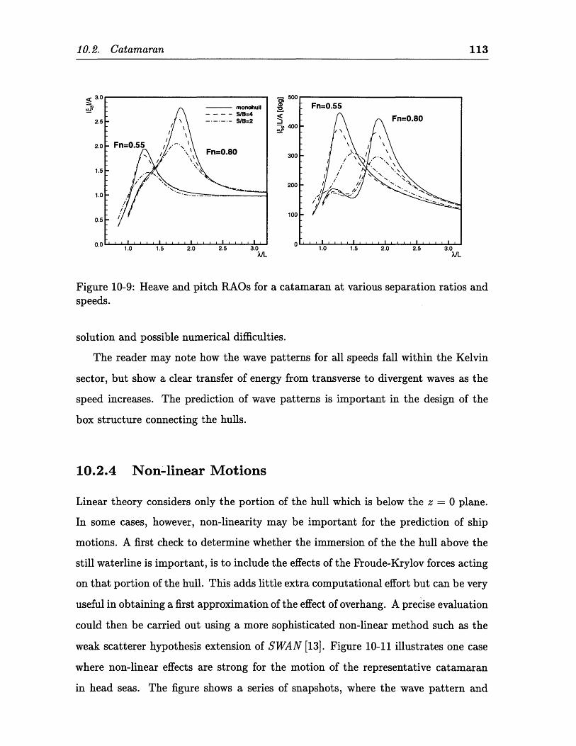
10-9 Heave and pitch RAOs for a catamaran at various separation ratios
and speeds. ................................ 113
10-10Steady wave patterns for a catamaran from moderate to high speeds. 114
10-11Snapshots of the submerged hull surface for a catamaran at F" = 0.3
in a regular head sea; and the corresponding time record for the linear
and non-linear heave motions. ...................... 115
xvii
xviii
A
C
CE
CD
Cd
Cf
CL
FD
Fn
G
9
H
L
M
mj
7t=
p
R,
Rx
SB
Sp
Sd
SF
xix
Nomenclature
aspect ratio
matrix of hydrostatic restoring coefficients
entrainment coefficient
induced drag coefficient
intersection of So with z = 0 plane
frictional coefficient
lift coefficient
wave-making resistance coefficient
Fourier transform of wave elevation
total hydrodynamic force
Froude number
Rankine source potential
acceleration of gravity
shape parameter
free wave spectrum of vessel
length of waterline
inertial matrix of body
m-term in the jth direction
unit normal vector
pressure
wave resistance
Reynolds number based on length x
exact wetted surface of body
linearized wetted surface of body
image of SB about z = 0 plane
portion of So below z = 0 plane
exact description free surface
(ni, r 2, n 3 )
Sp free surface in undisturbed position
Sp surface representing "thin" body (plate)
Sw surface representing vortex wake
Soo semi-infinite vertical plane below free surface, far downstream
s span
T (subscript) trailing edge of lifting surface or transom
U magnitude of mean velocity
Ve breathing velocity
W mean velocity of body
x = x1 coordinate in direction of mean body motion
y = X2 horizontal coordinate normal to direction of body motion
z = x3 vertical coordinate
a angle of attack
y flare angle of hull
A "jump" operator on dipole sheet
3* displacement thickness
3 displacement of body about mean position
E hull slenderness parameter
Sfree surface wave elevation
0 momentum thickness
NX wavenumber of wave propagating in x-direction
Ky wavenumber of wave propagating in y-direction
v kinematic viscosity
R = (4, 5, 6) rigid body rotation
T = (1, ~2, 3) rigid body translation
p density
a strength of source distribution
disturbance potential of basis flow
op perturbation flow velocity potential
TI total disturbance velocity potential
Part IBackground
The schooner yacht America (1851)
CHAPTER 1
INTRODUCTION
1.1 Motivation
A ship differs from any other large engineering structure in that - in addition to all
its other functions - it must be designed to move efficiently through the water with
a minimum of external assistance. Another requirement besides good smooth-water
performance, is that under average service conditions at sea, the ship shall not suffer
from excessive motions, wetness of decks, or lose more speed than necessary in bad
weather.
Although ships have been traversing the oceans for millennia, there has not always
been a systematic way of satisfying the above criteria. Designers have relied on
centuries of tradition and their own experience and intuition, but in order to actually
ensure the desirable ship performance, it is necessary to possess knowledge of the
hydrodynamics of the hull and the propulsion system.
Because of the complicated nature of ship hydrodynamics, early recourse was made
to experiments for its understanding. But even after model testing was revolutionized
by Froude in the 1860's, it still remains a very time-consuming and expensive process.
Ever since the advent of the digital computer, numerical methods have been gain-
ing popularity as an alternative to towing tank testing. The field has been rapidly
evolving over the past 15 years, ultimately leading to the development of fully three-
4 Chapter 1. Introduction
dimensional boundary integral element methods.
Such methods, also known as panel methods, discretize boundaries of the fluid
into elements with an associated singularity strength, impose appropriate boundary
conditions, and most use linear potential flow theory to attempt to numerically repro-
duce the flow past the ship. A class of such methods, which has produced especially
promising results, employs the Rankine source as the elementary singularity. It is
very flexible in the free surface conditions that it can enforce, and when combined
with a time-domain approach, can even be extended to include non-linear effects.
There are, however, several limitations of these methods that currently prevent
them from totally replacing the experiment as a primary means of evaluating a design.
One such restriction is that of geometric complexity. Present linear methods
have not had success in treating ships with deep transom sterns, for example. Also,
agreement with experiments has been questionable for hulls with significant flare,
or with overhang at the stern. Both the above characteristics are very common in
today's fleet of commercial ships and sailing yachts, and must be treated properly,
using a sound theoretical basis, while overcoming any numerical difficulties.
Hulls with thin appendages compared to the overall dimensions of the ship, are
another geometric complexity presenting a challenge for panel methods. Sails, off-
shore platform damping plates, and even rudders are a few such examples, where
an inordinate amount of panels are required to overcome the numerical difficulties
associated with the proximity of the surfaces on which elementary singularities are
distributed.
Another limitation is the fact that panel methods do not account for viscosity. The
interaction between the wave flow and the viscous boundary layer cannot be captured
with existing potential flow methods. This interaction is, however, inherently present
in towing tank tests'.
Many types of advanced marine vehicles such as catamarans, SWATH, and SES,
1Even in towing tank tests, however, this interaction might not be accurately evaluated due toscaling effects. In addition, such tests rely on the rather crude Froude hypothesis to determinethe residuary resistance. Therefore, a numerical method that accounts for viscous effects has thepotential of being more accurate than model tests.
1.2. Research History 5
operate with their hulls producing a significant amount of lift. In addition, ap-
pendages such as keels, rudders, and winglets are vital for the operation of sail-
ing yachts. Therefore, the treatment of circulation is another feature that would
enormously help in establishing panel methods as a design tool, especially since the
amount of experimental data available for non-conventional ships is limited.
This thesis will address all of the above issues, attempting to bring a Rankine
panel method closer to being a ship designer's primary tool for the hydrodynamic
evaluation of complex marine vehicles.
1.2 Research History
Boundary integral element methods form the basis of the majority of the computa-
tional algorithms for the numerical solution of the forces and wave patterns of bodies
traveling near the boundary between two fluids. In 1976-77, the work of Gadd [9]
and Dawson [7] ignited a class of such methods which use the Rankine source as
their elementary singularity. Known as Rankine panel methods, they distribute these
singularities on the discretized free surface, as well as on the body, and solve for their
unknown strengths.
The advantage of such methods is the freedom to impose a wide range of free
surface boundary conditions. This leads to a flexibility of linearization about a ba-
sis flow or even extension to the fully non-linear problem. In 1988, Sclavounos and
Nakos [31] presented an analysis for the propagation of gravity waves on a discrete
free surface which instilled confidence that such a method could faithfully represent
ship forces and wave patterns, despite the distortion of the wave system introduced
due to the free surface discretization. Their work led to the development of a fre-
accurately predicting the flow, as reported for several applications [32, 47].
The time domain formulation, and simultaneous solution of the equations of mo-
tion with the wave flow, is another feature which allows for the future inclusion of
non-linearities in the unsteady problem. Kring [18, 20] extended the work of Nakos
6 Chapter 1. Introduction
and Sclavounos to the time domain, preserving their methodology, thus taking ad-
vantage of the experience gained by the evolution of SWAN and ensuring that the
underlying numerical method faithfully represented the problems posed.
Such linear methods give reliable estimates of the motions, wave patterns, and
forces for most practical hull forms. But for certain extreme cases, such as ships with
large curvature or slope at the waterline, the linearized free surface conditions become
inconsistent. Recently, fully non-linear panel methods have been developed, which
remove the inconsistencies inherent in the linearization process. At present, however,
these methods are either not general enough, or too inefficient to be routinely used
for evaluating the performance of real applications. Xia [50], Ni [36], Jensen [15, 16],
and Raven [40] have developed methods which deal only with the problem of steady
motion. The transient method of Beck and Cao [1, 5], is more flexible but very
computationally intensive.
This study will be concerned with extending a linear panel method to include
viscous effects, lifting surfaces, and treatment of thin bodies and complex geometries
such as transom sterns. Thus, it will immediately become a practical tool of hydro-
dynamic design. The time-domain, boundary integral element approach will ensure
that as computer power increases in the future, the method will be readily extendible
to non-linear computations. In fact, some non-linear extensions have already been
incorporated. There is currently capability to include the effect of non-linearities such
as systems of active control and viscous roll damping [45], while the recent work of
Huang [13] based on a weak scatterer hypothesis has led to significant improvements
in the non-linear seakeeping problem.
1.3 Overview
As mentioned above, the present thesis will extend a Rankine panel method to include
viscous effects, and provide a means of treating lifting surfaces, thin bodies, and the
flow past transom sterns. These seemingly unrelated topics have as a common goal
to enable the ship designer to analyze the flow past complex hulls such as semi-
1.3. Overview
displacement ships, catamarans, and sailing yachts.
Part I provides the background theory and methodology which are necessary for
the extensions of the Rankine panel method, and consists of two chapters. Chapter 2
gives an overview of the basic time-domain Rankine panel method and chapter 3
reviews the method used for the calculation of the steady wave resistance and the
added resistance due to waves.
Part II presents the new contributions of this work. Chapter 4 extends the
method to include viscosity effects and their interaction with the wave flow. A direct
viscous-inviscid interaction algorithm is developed using the Rankine panel method
and an integral turbulent boundary-layer method. Chapter 5 gives a method to
treat free surface flows with lift, by modeling the trailing vortex wake and employing
an appropriate Kutta condition. Chapter 6 provides an extension for bodies with
infinitesimally small thickness by modeling them as dipole sheets. Finally, chapter 7
presents a solution for the numerical treatment of flows past deep transom sterns.
Part III presents some case studies, in which the above extensions are utilized
to assess the performance of various advanced marine vehicles. In chapter 8, the
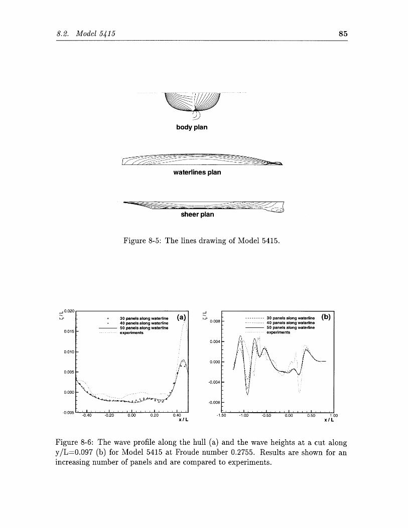
method is used with two conventional ships and is tested for convergence and for
agreement with experiments. Chapter 9 presents an extensive study of a sailing
yacht, including the aerodynamic forces and a full time-domain simulation of the
vessel under sail. Chapter 10 examines the forces, wave patterns and motions of a
semi-displacement ship and a catamaran.
8 Chapter 1. Introduction
CHAPTER 2
THE RANKINE PANEL METHOD
This chapter will give an overview of a time domain, linear Rankine panel method,
with the purpose of providing a framework on which the extensions of the following
chapters will be based. The problem is formulated in section 2.1, and the numerical
implementation in an efficient algorithm is given in section 2.2. For a more detailed
description, the reader may refer to the Ph.D. thesis of Kring [18].
2.1 Mathematical Formulation
2.1.1 Problem Definition
Figure 2-1 displays a vessel with wetted surface SB, interacting with the surface of
the sea, SF. It may have a mean forward speed, WI, and a reference frame (x, y, z) is
fixed to this steady motion. All quantities below are taken with respect to this frame
of reference.
The body may also perform time-dependent motions about this frame of reference
in the six rigid-body degrees of freedom. Its displacement 6, at position F = (x, y, z),
may then be written as
w7(, t) = T(t) + R(t) X = (2.1)
where T = (i, 2, 3) is the rigid body translation and R = ( 4, 5, 6) is the rigid
Z
0 Y x
Figure 2-1: A graphic representation of the problem
The Rankine Panel MethodChapter 2.
-1
2.1. Mathematical Formulation 11
body rotation.
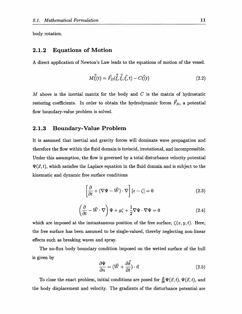
2.1.2 Equations of Motion
A direct application of Newton's Law leads to the equations of motion of the vessel.
M (t) = FD( , , , t) - C((t) (2.2)
M above is the inertial matrix for the body and C is the matrix of hydrostatic
restoring coefficients. In order to obtain the hydrodynamic forces FD, a potential
flow boundary-value problem is solved.
2.1.3 Boundary-Value Problem
It is assumed that inertial and gravity forces will dominate wave propagation and
therefore the flow within the fluid domain is inviscid, irrotational, and incompressible.
Under this assumption, the flow is governed by a total disturbance velocity potential
T (Y, t), which satisfies the Laplace equation in the fluid domain and is subject to the
kinematic and dynamic free surface conditions
+ (V - l) - V [z - ] = 0 (2.3)
(- V _1+g(+-V-V=0 (2.4)
which are imposed at the instantaneous position of the free surface, ((x, y, t). Here,
the free surface has been assumed to be single-valued, thereby neglecting non-linear
effects such as breaking waves and spray.
The no-flux body boundary condition imposed on the wetted surface of the hull
is given by
= (W + -n (2.5)an a
To close the exact problem, initial conditions are posed for T4(Y, t), X(X, t), and
the body displacement and velocity. The gradients of the disturbance potential are
12 Chapter 2. The Rankine Panel Method
also required to vanish at a sufficiently large distance from the vessel at any given
finite time.
2.1.4 Basis Flow
The flow is linearized about a dominant basis flow. There are two linearizations
that are commonly applied to this three-dimensional problem. One is the classical
Neumann-Kelvin linearization, where a uniform stream is taken as the basis flow. For
most realistic hull forms, however, the best results are obtained by linearizing about
a double-body flow, as first proposed by Gadd [9] and Dawson [7].
There is a choice of methods for the solution of the double-body flow using a panel
method. One such method consists of distributing sources on the body boundary SD,
and its mirror image about the z = 0 plane Sy., and then using the boundary
condition (2.5) to derive an integral equation for their unknown strengths, a().
J() dx' = W i (2.6)sjBUSR, On
where G(I; Z) = is the Rankine source potential, and sES,
Note, however, that if the double body flow involves circulation, then a solution
cannot be found in terms of a pure Rankine source distribution on the body. In
this case it is necessary to use either dipoles or vortices in addition to sources. The
application of Green's second identity, together with the body boundary condition
(2.5), leads to the potential formulation of the double-body, which may be expressed
as follows
2vbG5- JJ) - (f n') G(X Y) dx' +
I(f Sus 4() ( dx' = 0 (2.7)
where (P is the disturbance potential of the double-body flow and xESp.
This method will be extended in section 5.2.2 for the case of a flow with circulation.
2.1. Mathematical Formulation 13
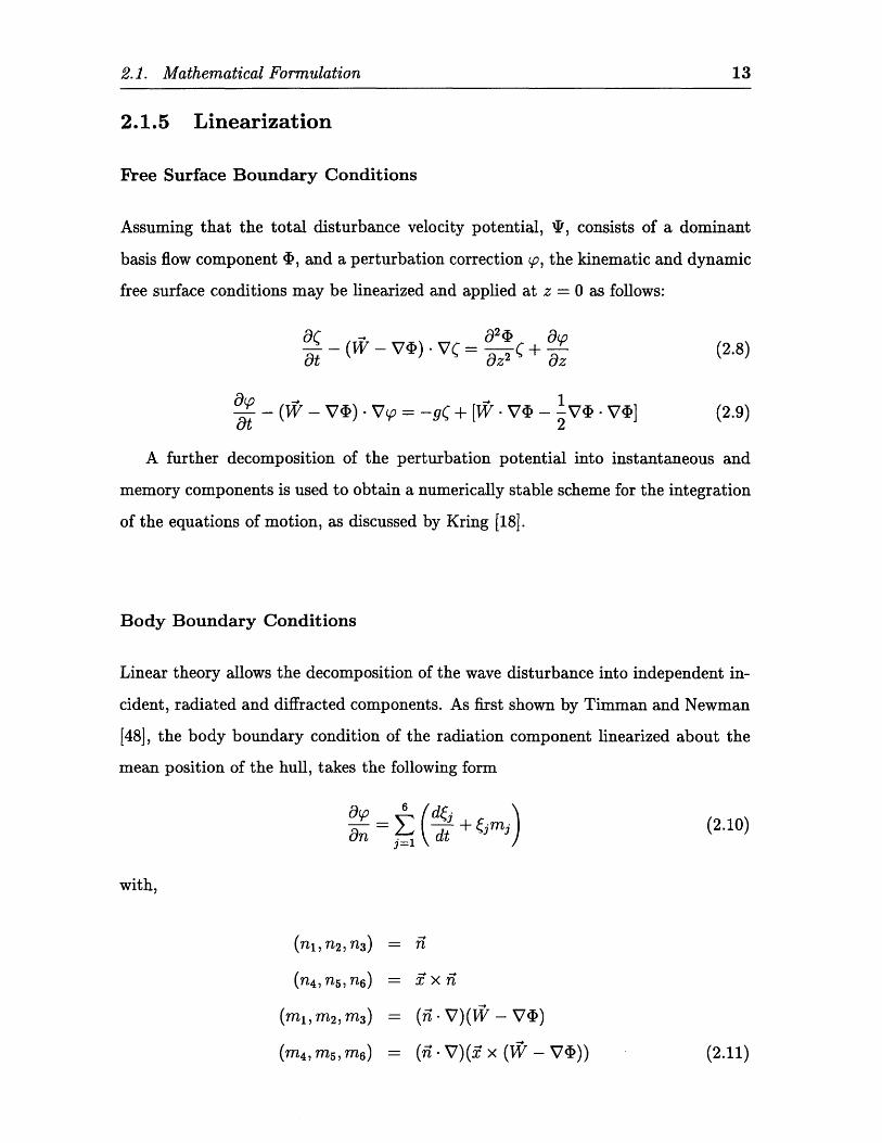
2.1.5 Linearization
Free Surface Boundary Conditions
Assuming that the total disturbance velocity potential, T, consists of a dominant
basis flow component 4, and a perturbation correction W, the kinematic and dynamic
free surface conditions may be linearized and applied at z = 0 as follows:
(W - V) • V( = + (2.8)at az2 az
-p (W - V() - V = -g~ + [V - V4 - 1-V( - V4)] (2.9)at 2
A further decomposition of the perturbation potential into instantaneous and
memory components is used to obtain a numerically stable scheme for the integration
of the equations of motion, as discussed by Kring [18].
Body Boundary Conditions
Linear theory allows the decomposition of the wave disturbance into independent in-
cident, radiated and diffracted components. As first shown by Timman and Newman
[48], the body boundary condition of the radiation component linearized about the
mean position of the hull, takes the following form
On ( d + jmj) (2.10)
with,
(ni, n 2 ,n 3) =
(n4, i 5,n 6) =x x n
(m , m,m2 ) = (.v)( - Vi,)
(m4, i 5 , , 6 ) = (ii. V)(7 x (W - V4)) (2.11)
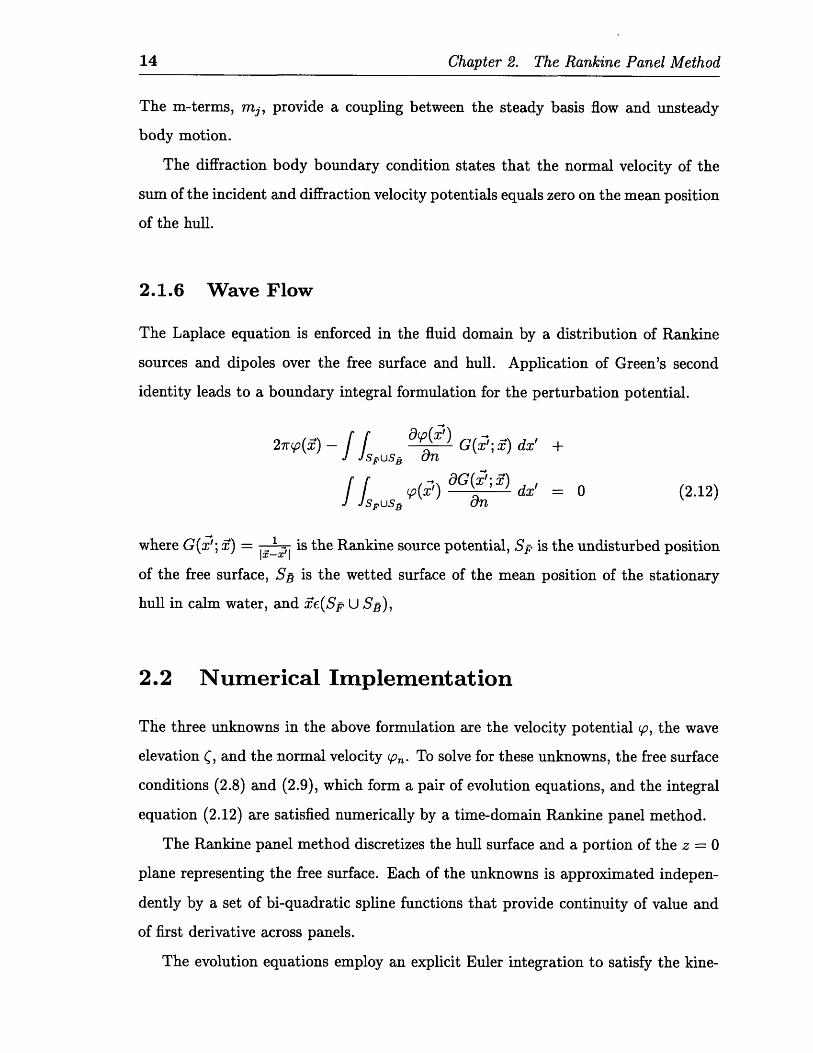
The m-terms, mj, provide a coupling between the steady basis flow and unsteady
body motion.
The diffraction body boundary condition states that the normal velocity of the
sum of the incident and diffraction velocity potentials equals zero on the mean position
of the hull.
2.1.6 Wave Flow
The Laplace equation is enforced in the fluid domain by a distribution of Rankine
sources and dipoles over the free surface and hull. Application of Green's second
identity leads to a boundary integral formulation for the perturbation potential.
27rp() - f us a G(; Y) dx' +
S p(1) G( ;) dx' = 0 (2.12)f spus an
where G(5; :) = is the Rankine source potential, Sp is the undisturbed position
of the free surface, Sf is the wetted surface of the mean position of the stationary
hull in calm water, and fE(Sp U SB),
2.2 Numerical Implementation
The three unknowns in the above formulation are the velocity potential 9, the wave
elevation C, and the normal velocity Vn,. To solve for these unknowns, the free surface
conditions (2.8) and (2.9), which form a pair of evolution equations, and the integral
equation (2.12) are satisfied numerically by a time-domain Rankine panel method.
The Rankine panel method discretizes the hull surface and a portion of the z = 0
plane representing the free surface. Each of the unknowns is approximated indepen-
dently by a set of bi-quadratic spline functions that provide continuity of value and
of first derivative across panels.
The evolution equations employ an explicit Euler integration to satisfy the kine-
14 Chapter 2. The Rankine Panel Method
2.2. Numerical Implementation 15
matic free surface condition and an implicit Euler integration to satisfy the dynamic
free surface boundary condition.
A numerical, wave-absorbing beach is used to satisfy the radiation condition, since
only a finite portion of the free surface is considered by the panel method.
Thus, a solution for the wave flow is produced and the equations of motion (2.2)
are integrated at each time step in order to satisfy the radiation body boundary
conditions.
A more detailed discussion of the formulation, numerical method, and applications
can be found in the work of Kring [18], Nakos and Sclavounos [31], and Sclavounos
et al.[45, 44]
16 Chapter 2. The Rankine Panel Method
CHAPTER 3
WAVE RESISTANCE
One of the most practical applications of panel methods, is the prediction of the wave
forces after the flow field has been solved.
In light of the three-dimensional Rankine panel method considered, this chapter
will review a consistent definition of wave resistance for the linearized problem, and
will introduce means of calculating the added resistance due to waves.'
3.1 Calm Water Resistance
The wave-making resistance of a ship is the net fore-and-aft force upon the ship due
to the fluid pressure acting normally on all parts of the hull. This pressure may be
readily obtained from Bernoulli's equation, after having determined the potential flow
from the solution of the boundary value problem which has been formulated in the
preceding chapter.
Due to the linearization of the problem about the calm water surface, it is neces-
sary to decompose the wetted surface into the portion Sp which lies beneath z = 0,
and an extra surface 6 SB, which accounts for the difference between the exact wetted
surface and Sg. The integration of the pressure over JSB, often referred to as the run-
'The panel method on which this work has been based was actually modified to perform thewave and added resistance calculations. It was not felt, however, that this constituted an originalcontribution and is thus discussed here as part of the background theory and methodology.
18 Chapter 3. Wave Resistance
up, may be collapsed into a line integral. This integral is of magnitude proportional
to the square of the wave elevation, and is therefore inconsistent with the linearization
of the free surface conditions (2.8), (2.9) which omit terms of comparable order.
For surface-piercing bodies, the only consistent definition of the linearized wave
resistance by pressure integration is the one adopted by thin-ship theory, where the
assumption of geometrical slenderness is employed in order not only to drop the
quadratic pressure terms of the perturbation flow, but also to linearize the hull thick-
ness effect by collapsing the body boundary condition on the hull centerplane.
On the other hand, for full shaped vessels, the quadratic terms of the perturbation
flow in Bernoulli's equation and in the run-up are considerable and their omission is
found to cause over-prediction of wave resistance, in a fashion similar to the perfor-
mance of thin-ship theory.
The solution is given by Nakos and Sclavounos [33], who show that the only
consistent definition of the wave resistance with the linearization of the problem
follows from conservation of momentum and not from pressure integration.
The wave resistance, as defined above, may be calculated by applying the momen-
tum theorem to a control volume bounded by the exact wetted surface of the hull, by
the exact position of the free surface, and by a closing surface at infinity. By virtue of
the radiation condition, the closing surface may be replaced by a vertical plane, S,,
normal to the ship axis at a large distance downstream. Taking into consideration
the asymptotically small magnitude of the wave disturbance in the far-field, it follows
that
pg_ -_ 2 0, O P 2 22
RJcI ( d d- - - dS (3.1)2 c 2 X ay 8z
where Cd is the intersection of So with the z = 0 plane, and Sd is the part of Soo
lying below z = 0.
Equation (3.1) may be evaluated either in terms of far-field quantities through
wave-cut analysis, or in terms of near-field quantities through pressure integration.
3.1. Calm Water Resistance 19
3.1.1 Wave Cut Analysis
The principal properties of the transverse wave cut method are briefly reviewed below.
Further details may be found in Eggers et al [8].
Consider a cut of the wave pattern perpendicular to the steady track of the vessel
for -oo < y < +oo. The transverse Fourier Transform of the wave elevation, ((x, y)
and its x-derivative are given by (3.2) and (3.3) respectively.
/+O0.F(X, ,y) = J (x, y)eydy (3.2)
-oo
Fx(X, y) ey dy (3.3)
In the limit as x -- + 00 the vessel's free wave spectrum is defined as
In the present Rankine panel method, however, the double-body flow with zero
flux through the boundaries has properties which are needed for the evaluation of
the m-terms2 . Modifying the basis flow is not, therefore, formally correct and will be
avoided.
4.3.3 Kinematic Free Surface Boundary Condition
The kinematic free surface boundary condition has been given in (2.3) and states that
a fluid particle on the free surface always remains on the free surface. This implies
that there is no flux across the exact position of the free surface. In order to account
for the presence of a boundary layer in the wake, the above condition is modified to
allow a flux per unit area across the free surface, equal to the breathing velocity.
dt + (V -l ) -V [z - (] = Ve (4.11)
Equation (4.11) is approximate and cannot be imposed at the exact instantaneous
position of the free surface, ((x, y, t). It is, however, valid when applied to the linear
problem as given in section 2.1.5, where the boundary condition is linearized about
a basis flow 4, and applied on the z = 0 plane. The modification to the linearized
kinematic free surface boundary condition is then derived in terms of the breathing
velocity as follows
(W - V ) - V( = (+ - - Ve (4.12)t az2 az
The above equation replaces (2.8) as the perturbation flow kinematic boundary
condition. The dynamic free surface boundary condition remains unaltered, since the
pressure across the boundary-layer is assumed to be constant.
2 As shown by Nakos [30], the evaluation of second order derivatives of the basis flow potential onthe hull may be avoided when calculating the influence of the m-terms, by making use of a theoremdue to Ogilvie and Tuck [37]. This theorem may be used, however, only under the condition of zeroflux of the basis flow through the surface of the body. The double-body flow does indeed satisfy thiscondition, but the aspiration model does not.
~4. The Coupling Algorithm 33
Figure 4-1: A flowchart of the coupling algorithm
4.4 The Coupling Algorithm
The procedure used to combine the solutions of the flow in the viscous and inviscid
regions is known as the coupling algorithm. Algorithms which have been used in two
dimensions include direct, inverse, semi-inverse, quasi-simultaneous, and simultaneous
coupling. Since the present method is a first attempt at the coupling of viscosity with
inviscid three-dimensional free surface flows, the simplest approach, a direct coupling
algorithm, was used. This method has been proven to converge, provided separation
is not encountered. In the field of aeronautical engineering, full three-dimensional
direct coupling methods have been developed by Lazareff and Le Balleur [23] for
transonic flow over finite wings.
A schematic description of the method used in this study to combine the viscous
and inviscid solutions is presented in figure 4-1. This coupling algorithm is described
in more detail below.
* Potential flow solution : The potential flow panel method can produce a
pressure distribution on the body by ignoring the effect of the boundary-layer,
4.4. The Coupling Algorithm 33
which will be relatively close to the pressure distribution of the full viscous flow.
The velocities on the body and free surface are then recorded for use by the
boundary-layer model.
* Streamline tracing : The output velocities from the panel method are used to
trace streamlines along the body and into the wake. The velocity distribution
on each streamline is recorded for input to the boundary-layer model.
* Viscous flow solution : The integral turbulent boundary-layer method (ap-
pendix A) uses the velocity distribution on each streamline to produce a solu-
tion. This solution consists of a distribution of the main integral parameters
along each streamline which will in turn be used to modify the potential flow
solution.
* Modification of the potential flow problem : As shown in section 4.3, basic
integral parameters of the boundary-layer solution may be used to compute an
effective normal velocity on the body and the free surface. This normal velocity,
to be imposed by the inviscid flow boundary conditions on each panel of the
input geometry, is found by interpolating V, (4.9) between streamlines.
* Iteration : The potential flow is then solved once again, taking breathing ve-
locities into account and new streamlines are traced. This procedure is repeated,
typically two to three times, until a converged solution is reached.
4.5 Viscous Force Calculations
This section reviews two methods for calculating the viscous resistance of a three-
dimensional body using the integral turbulent boundary-layer method described above.
The first one is based on a shear stress integration and the other is based on conser-
vation of momentum considerations.
34 Chapter 4. Viscous Effects
4.5. Viscous Force Calculations
4.5.1 Shear Stress Integration
One of the parameters of the integral turbulent boundary-layer method is the skin
friction coefficient C, which is defined as the shear stress on the body surface nor-
malized by pU2. The integration of this shear stress over the wetted surface of the
body results in the total viscous force acting on the hull.
Fv== p U2 Cfcos a dS (4.13)
where a is the angle between the x-axis and the tangential vector to the body in the
streamwise direction.
4.5.2 Conservation of Momentum
Alternatively, the two-dimensional drag associated with a single streamline may be
found by conservation of momentum and then integrated over the width of the viscous
flow to get the total viscous drag.
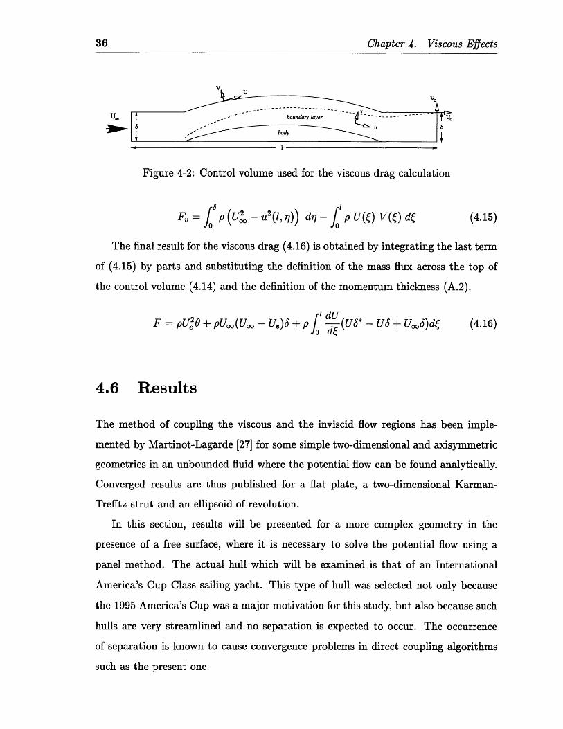
What follows is the derivation of a method for calculating the two-dimensional
viscous drag, given the integral parameters of the boundary-layer up to a point in
the wake downstream of the body. The control volume considered is shown in figure
4-2 and extends longitudinally from far upstream of the body to a point in the wake.
The thickness is constant and equal to the thickness of the boundary-layer 6, at the
downstream end of the control volume. Let Ue, 6, 6", and 0 denote the quantities
at the downstream end of the control volume. U, is the free stream velocity. The
coordinates , 77, and the fluid velocities at the edge of the boundary layer U, V are,
respectively, locally tangent and locally normal to the body.
By applying the principles of conservation of mass and momentum in the control
volume, and using the definition of the displacement thickness (A.1), equations (4.14)
and (4.15) follow.
foVd = [Uoo - u(,,)] d
= Ue6* - (Ue - Uoo)6 (4.14)
36 Chapter ~j. Viscous Effects
Figure 4-2: Control volume used for the viscous drag calculation
F, = p (U - u2(l1, q)) dr - fjp U(6) V(6) d (4.15)
The final result for the viscous drag (4.16) is obtained by integrating the last term
of (4.15) by parts and substituting the definition of the mass flux across the top of
the control volume (4.14) and the definition of the momentum thickness (A.2).
2ot + UGd _ dU(4.16)F = pUO + pUo(Uo - Ue)6 + p -(U6* - U6+Uo6)d (4.16)
4.6 Results
The method of coupling the viscous and the inviscid flow regions has been imple-
mented by Martinot-Lagarde [27] for some simple two-dimensional and axisymmetric
geometries in an unbounded fluid where the potential flow can be found analytically.
Converged results are thus published for a flat plate, a two-dimensional Karman-
Trefftz strut and an ellipsoid of revolution.
In this section, results will be presented for a more complex geometry in the
presence of a free surface, where it is necessary to solve the potential flow using a
panel method. The actual hull which will be examined is that of an International
America's Cup Class sailing yacht. This type of hull was selected not only because
the 1995 America's Cup was a major motivation for this study, but also because such
hulls are very streamlined and no separation is expected to occur. The occurrence
of separation is known to cause convergence problems in direct coupling algorithms
such as the present one.
36 Chapter 4. Viscous Effects
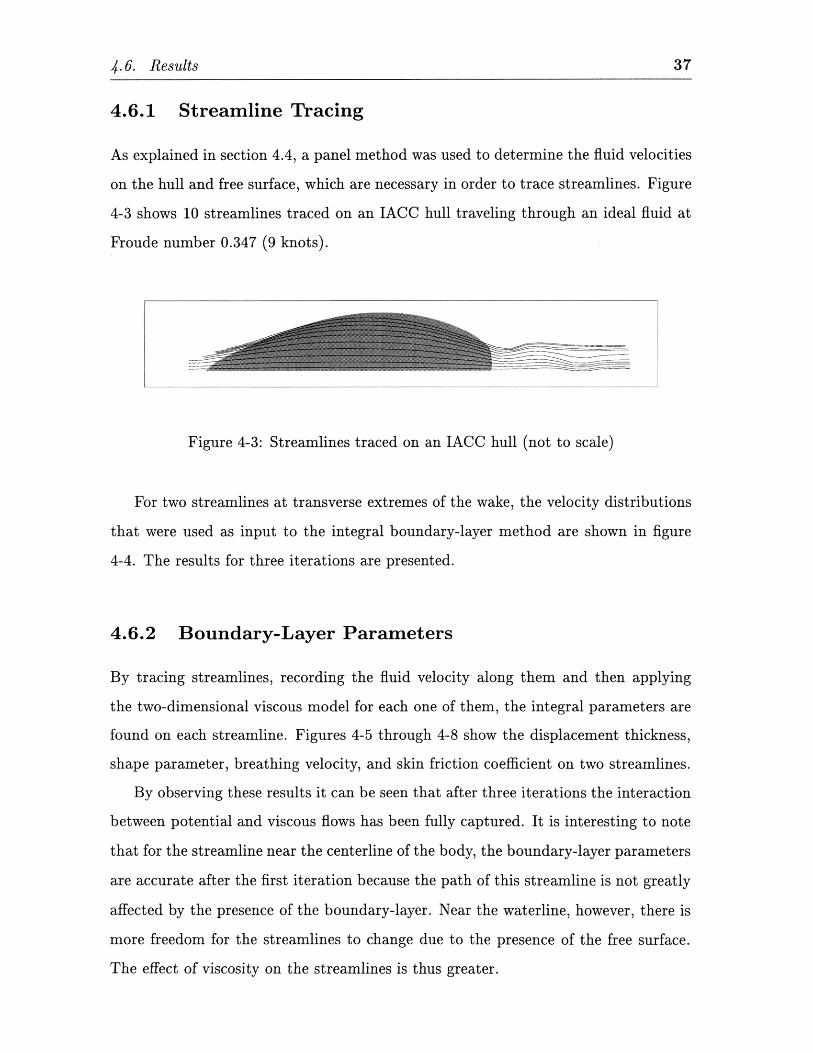
4.6.1 Streamline Tracing
As explained in section 4.4, a panel method was used to determine the fluid velocities
on the hull and free surface, which are necessary in order to trace streamlines. Figure
4-3 shows 10 streamlines traced on an IACC hull traveling through an ideal fluid at
Froude number 0.347 (9 knots).
Figure 4-3: Streamlines traced on an IACC hull (not to scale)
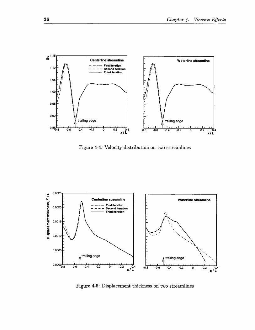
For two streamlines at transverse extremes of the wake, the velocity distributions
that were used as input to the integral boundary-layer method are shown in figure
4-4. The results for three iterations are presented.
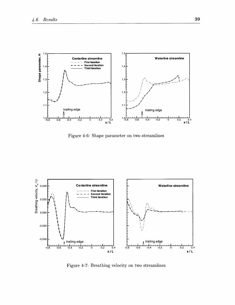
4.6.2 Boundary-Layer Parameters
By tracing streamlines, recording the fluid velocity along them and then applying
the two-dimensional viscous model for each one of them, the integral parameters are
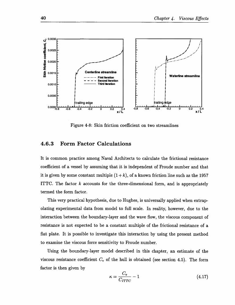
found on each streamline. Figures 4-5 through 4-8 show the displacement thickness,
shape parameter, breathing velocity, and skin friction coefficient on two streamlines.
By observing these results it can be seen that after three iterations the interaction
between potential and viscous flows has been fully captured. It is interesting to note
that for the streamline near the centerline of the body, the boundary-layer parameters
are accurate after the first iteration because the path of this streamline is not greatly
affected by the presence of the boundary-layer. Near the waterline, however, there is
more freedom for the streamlines to change due to the presence of the free surface.
The effect of viscosity on the streamlines is thus greater.
4.6. Results 37
38 Chapter 4. Viscous Effects
0.4x/L
Figure 4-4: Velocity distribution on two streamlines
Figure 4-5: Displacement thickness on two streamlines
38 Chapter 4. Viscous Effects
4.6. Results
-0.6 -0.4 -0.2 0 0.2 0.4x/L
Figure 4-6: Shape parameter on two streamlines
> 0.040
o
> 0.0200)cC ..
)mO 0.000
-0.020 F
-0.040
-0.8 -0.6 -0.4 -0.2
x/L0 0.2 0.4
x/L
Figure 4-7: Breathing velocity on two streamlines
39
1.4
1.3
1.2
1.1
1.0YOPo
Waterline streamline
-aig d
-/-I
- trailing edge.. .. I , , , , I, , , , I , , , , 1l ., ,l ,
.8
Waterline streamline
-\IS I\
\ I
: K r i I, J , I... i ..
40 Chapter 4. Viscous Effects
0.0030
O 0.0025 /
o
0.0020 --
. 0.0015 Centerline streamlineto) ------- First iteration Waterline streamline
- Second iteration0.0010 Third iteration
0.0005
trailing edge trailing dge0 .0 0 0 0 ' .. . I I I i , I ' . . . , I . . .
Figure 4-8: Skin friction coefficient on two streamlines
4.6.3 Form Factor Calculations
It is common practice among Naval Architects to calculate the frictional resistance
coefficient of a vessel by assuming that it is independent of Froude number and that
it is given by some constant multiple (1 + k), of a known friction line such as the 1957
ITTC. The factor k accounts for the three-dimensional form, and is appropriately
termed the form factor.
This very practical hypothesis, due to Hughes, is universally applied when extrap-
olating experimental data from model to full scale. In reality, however, due to the
interaction between the boundary-layer and the wave flow, the viscous component of
resistance is not expected to be a constant multiple of the frictional resistance of a
flat plate. It is possible to investigate this interaction by using the present method
to examine the viscous force sensitivity to Froude number.
Using the boundary-layer model described in this chapter, an estimate of the
viscous resistance coefficient C, of the hull is obtained (see section 4.5). The form
factor is then given byC,S C 1 (4.17)
CITTC
4.6. Results 41
J 0.02
So0.00oo
E -0.02
-0.04 -
-0.06
-0.08
0.0 0.1 0.2 0.3 0.4Fn
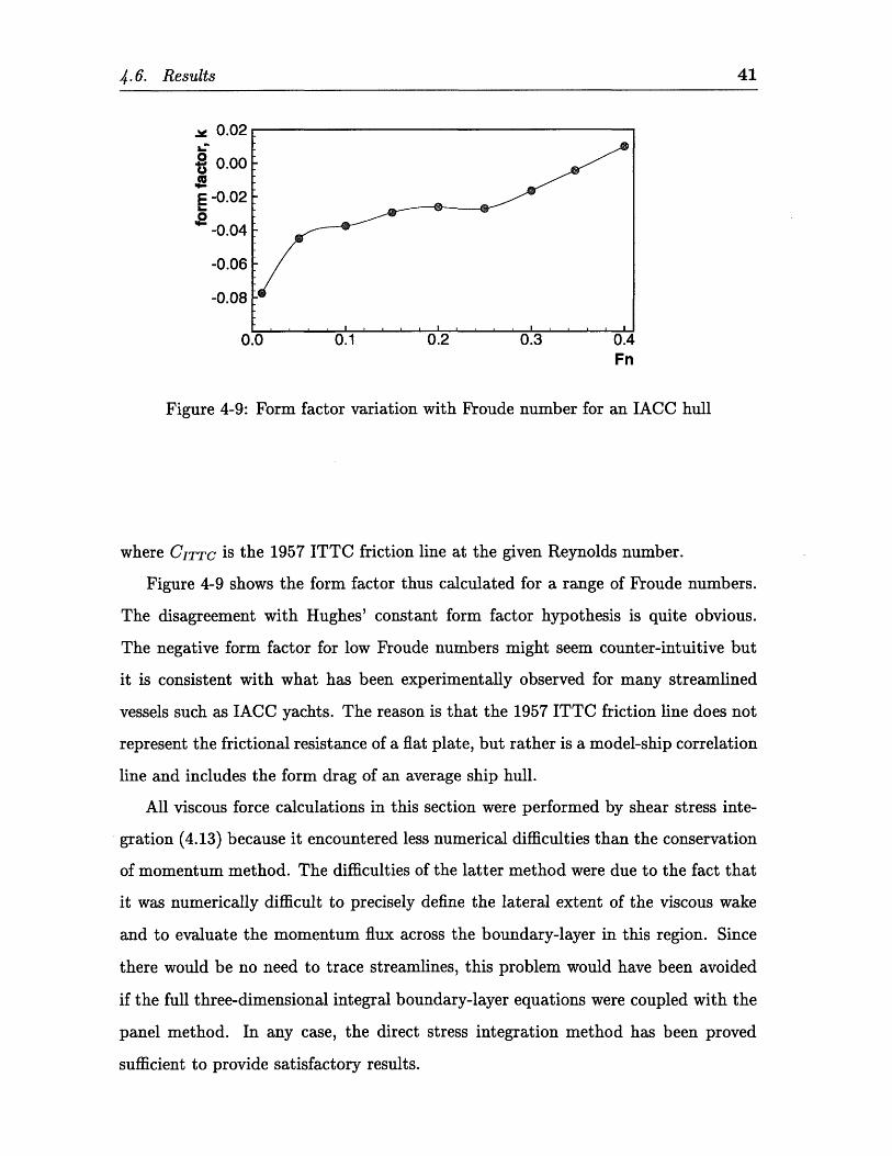
Figure 4-9: Form factor variation with Froude number for an IACC hull
where CITTC is the 1957 ITTC friction line at the given Reynolds number.
Figure 4-9 shows the form factor thus calculated for a range of Froude numbers.
The disagreement with Hughes' constant form factor hypothesis is quite obvious.
The negative form factor for low Froude numbers might seem counter-intuitive but
it is consistent with what has been experimentally observed for many streamlined
vessels such as IACC yachts. The reason is that the 1957 ITTC friction line does not
represent the frictional resistance of a flat plate, but rather is a model-ship correlation
line and includes the form drag of an average ship hull.
All viscous force calculations in this section were performed by shear stress inte-
gration (4.13) because it encountered less numerical difficulties than the conservation
of momentum method. The difficulties of the latter method were due to the fact that
it was numerically difficult to precisely define the lateral extent of the viscous wake
and to evaluate the momentum flux across the boundary-layer in this region. Since
there would be no need to trace streamlines, this problem would have been avoided
if the full three-dimensional integral boundary-layer equations were coupled with the
panel method. In any case, the direct stress integration method has been proved
sufficient to provide satisfactory results.
42 Chapter 4. Viscous Effects
6 0.03 .(a) - inviscid c (b) -A-- inviscid
- - - -viscous ----- viscous0 .02 ........................... h u ll
0.00
-0.01
-0.02
-0.03 .
-0.04 -
-0.05 r I I -1.0 -0.5 0.0 0.5 0.1 0.2 0.3 04
x/L U /1(gL)
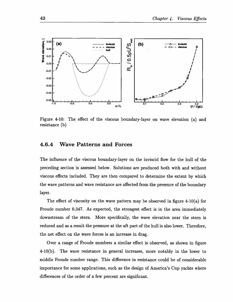
Figure 4-10: The effect of the viscous boundary-layer on wave elevation (a) andresistance (b)
4.6.4 Wave Patterns and Forces
The influence of the viscous boundary-layer on the inviscid flow for the hull of the
preceding section is assessed below. Solutions are produced both with and without
viscous effects included. They are then compared to determine the extent by which
the wave patterns and wave resistance are affected from the presence of the boundary
layer.
The effect of viscosity on the wave pattern may be observed in figure 4-10(a) for
Froude number 0.347. As expected, the strongest effect is in the area immediately
downstream of the stern. More specifically, the wave elevation near the stern is
reduced and as a result the pressure at the aft part of the hull is also lower. Therefore,
the net effect on the wave forces is an increase in drag.
Over a range of Froude numbers a similar effect is observed, as shown in figure
4-10(b). The wave resistance in general increases, more notably in the lower to
middle Froude number range. This difference in resistance could be of considerable
importance for some applications, such as the design of America's Cup yachts where
differences of the order of a few percent are significant.
4.7 Conclusions and Recommendations
A method of coupling an integral turbulent boundary-layer method with a Rankine
panel method has been devised and implemented. The benefits of this approach is
that both major components of the total drag of a ship, the viscous and wave drag,
may be estimated with better accuracy than if they were considered separately.
The viscous force calculations demonstrate shortcomings in the traditional ap-
proach of assuming that a ship's viscous resistance coefficient is equal to a constant
multiple of the resistance coefficient of a flat plate. In addition, the wave force
calculations suggest that the interaction between the free surface and the viscous
boundary-layer can be important at certain Froude numbers.
The method is, however, computationally intensive, as it is necessary to solve
the inviscid flow problem at least two times in order to converge to a solution that
satisfies both the integral turbulent boundary-layer equations and the potential flow
boundary value problem.
Also, there are several restrictions of this method, which invite the attention of
future work.
* Problems are expected to occur if separation is encountered in the flow. The
direct coupling algorithm used is known to fail in such situations. The solu-
tion would be to employ a simultaneous coupling algorithm, as in the work of
Milewski [28] for an unbounded fluid. But even then, the flow past bluff bodies
with open separation would not be able to be treated.
* Currently, the method assumes negligible crossflow, which can be a rather severe
approximation for realistic flows past ship hulls. The three-dimensional integral
boundary-layer equations could be used to rectify this situation, at the expense
of a more elaborate boundary-layer solution scheme.
* For all the above analysis, a steady flow is assumed. If the viscous effects are
to be included for unsteady flows, the integral boundary-layer equations need
to be solved at each time step of the panel method. Unless a more intelligent
4.7. Conclusions and Recommendations 43
44 Chapter 4. Viscous Effects
coupling scheme is devised, this would be too computationally demanding for
real applications.
CHAPTER 5
LIFTING SURFACES
This chapter presents an extension of the Rankine panel method for free surface flows
with lift.
5.1 Introduction
Some special types of ships, such as sailboats and hydrofoil craft, operate with their
hulls designed to produce a significant amount of lift. In addition, multi-hulled vessels,
such as catamarans, may have a certain amount of interaction between their hulls,
which cannot be accurately predicted without considering them as lifting surfaces.
The ability to include lifting surfaces is therefore essential, and it needs to be included
in any method intended for the evaluation of such complex hull-forms.
Panel methods were first applied to the aeronautical industry, and it was, there-
fore, not long before they were further developed to take the lift and induced drag of
airplane wings into account [12]. Such methods have been adopted by Naval Archi-
tects in the past, and have been directly applied to the flow past ship hulls, neglecting
the presence of the free surface'. This approach was used by Greeley and Cross-Whiter
[10] to design keels for the 1987 America's Cup campaign, for example.
1A zero Froude number approximation is needed for this approach, which replaces the free surfaceby a rigid wall.
46 Chapter 5. Lifting Surfaces
More recently, several steady flow panel methods have been extended to include
the interaction of lift-producing hulls with the free surface [49, 41, 14). All these
methods introduce a lift force by distributing vortices or dipoles on the body or the
mean camber line. In addition, they impose a Kutta condition of flow tangency or
pressure equality at the trailing edge, and introduce a trailing vortex system shed
into the flow to satisfy Kelvin's theorem.
This chapter will use a similar approach to solve the steady or unsteady lifting
problem in the time-domain. Section 5.2 explains how to incorporate lifting surfaces
in the formulation of the boundary value problem. The numerical implementation is
given in section 5.3, and some simple cases are examined for validation purposes in
section 5.4.
5.2 Formulation
Section 2.1 has formulated the problem of the flow without circulation. Extending
the numerical implementation described therein, changes are needed in both the basis
and perturbation flows.
5.2.1 Wake Condition
The wake behind the lifting surface is modeled by a free vortex sheet. This sheet is
considered infinitesimally thin and is composed of two surfaces, S + and Sw, which
occupy the same position but have opposite normal direction.
The wake surface is assumed to be fixed in the vessel coordinate system and its
shape follows by tracing the lifting surface trailing edge directly downstream. The two
surfaces representing the wake are combined into a single jump surface, Sw, which
in the present method is represented by a dipole sheet. In what follows, A is the
operator which denotes the jump in a quantity across the wake, and the superscripts
"+" and "-" denote quantities on the surfaces S + and Sw, respectively.
Relating circulation around the body to the potential jump across the wake,
Morino [29] proposed a linear Kutta condition which specifies the strength of the
dipole sheet in the wake. This condition states that the potential jump in the wake
just downstream of the trailing edge must equal the difference in potential on the
body on each side of the trailing edge. This is equivalent to a statement of continuity
of potential from the body into the wake. A similar idea is successfully used for the
treatment of deep transom sterns in chapter 7.
If the trailing edge has finite thickness, the collocation points of the body panels on
opposite sides of the trailing edge may have different values of free-stream potential.
It is then necessary to apply a correction to the Morino condition, as proposed by
Lee [24], which requires the potential jump in the wake to be equal to the difference
in total potential at the collocation points of the panels at the trailing edge.
A'I(Zw, t) = F(7B, t)+ - (B,t)- - 'rTE (5.1)
where wcWSw, and 'BSB at the intersection of SB with Sw. TE is the vector joining
the collocation points of the two trailing edge panels.
The wake can sustain no forces so there must be no jump in pressure, p( , t),
across the sheet
Ap = p(I, t) - p(i, t)- = 0 (5.2)
Using Bernoulli's equation and linearizing about the free stream, an expression
for the potential jump AT(, t) in the wake, may be obtained.
-V( J)= 0 (5.3)at
Although accurate for two-dimensional sections with small exit angles, this lin-
earization may not be satisfactory for three dimensional problems with significant
cross-flow [24]. In this case, a non-linear Kutta condition is required, explicitly stat-
ing that the pressure jump in the wake must vanish.
However, for high aspect ratio lifting surfaces such as sailboat keels and rudders,
the cross-flow is not expected to have a significant effect at most sections of the
foil. Indeed, examination of typical foils at an angle of attack of less that 10 degrees
5.2. Formulation 47
revealed that the linear Morino condition also forced the pressure jump at the trailing
edge very close to zero in most cases.
One exception is the vicinity of the intersection of the vortex wake with the free
surface, where there is an inconsistency between the wake and free surface condition
linearizations. The linear Morino condition was derived from the linearization of the
flow about the free stream, with the intention of setting the pressure jump in the wake
equal to zero. But in general, the basis flow which is used to linearize the free surface
conditions leads to a finite pressure jump across the wake. Through the dynamic free
surface condition, this translates to a jump in the wave elevation. It is interesting to
note is that this jump is also experimentally observed in real flows.
For lower aspect ratio foils which are not expected to operate under high loading,
such as the demi-hulls of a catamaran, it has been shown by Kring [19] that the above
linearization is satisfactory.
5.2.2 Basis Flow
As seen in section 2.1.4, the source formulation for the solution of the double-body
flow may not be used when circulation is present. Instead, the potential formulation
(2.7) is modified to account for the presence of a wake sheet.
Collapsing the wake surfaces S+ and Sw into a single surface, and imposing a
continuous normal velocity across it, Green's second identity yields an expression for
the unknown potential on the body;
27r( )) - f s( f f )G( ;Y) dx' +
sB () G (OG ; ) dx' +
S A(x) G(n d' = 0 (5.4)
The potential jump on the dipole sheet is also unknown, but is determined in
terms of the potential on the body through the Morino condition (5.1). Since the
flow is steady, the jump is merely required to be constant in the streamwise direction
48 Chapter 5. Lifting Surfaces
5.3. Numerical Implementation 49
according to (5.3).
5.2.3 Wave Flow
The linearization of the problem about the basis flow does not differ from the case
without lift, with the body and free surface boundary conditions as given in section
2.1.5.
In a similar manner as for the basis blow, the governing equations of the wave
flow expressed in boundary-integral form (2.12) may be modified to account for the
presence of a vortex wake sheet;
f a)o( ) G(x') dx' +J JSPUSR a
spus () On +
I 'S () = 0 (5.5)
where fe(Sp U SB).
The jump in potential in the wake is time-dependent in this case, as dictated by
(5.3).
5.3 Numerical Implementation
The numerical implementation of the method including vorticity is along the lines
given in section 2.2. There is an additional number of unknowns in the integral
equation, equal to the number of panels immediately aft of the trailing edge of the
lifting surface. Each of those panels is associated with a pair of panels on the body, and
the additional equations required to find a solution follow from the Morino condition
(5.1).
The potential jump on the rest of the panels of the wake is determined separately
from an explicit Euler integration of (5.3), with upwind differencing for the evaluation
of the spatial derivatives. The upwinding adds some damping to the vortex wake
system, but this does not affect the solution in any visible way over the range of
practical wave frequencies tested. The free surface, which is much more critical to
the solution, is still free of damping. Another alternative, which is to use central
differencing for the evaluation of the spatial derivatives in the wake, is impractical
due to the severe restrictions in panel length and time step in order to achieve stability.
The actual value of the potential on the two sides of the wake need not be de-
termined for this problem, although it would be possible, as described in section
6.1.
In some cases of problems with lift that were studied, the bi-quadratic spline func-
tions on the body were found to have an oscillatory behavior about the true solution.
This was observed especially for foils with sharp leading edges under significant angles
of attack and was due to the inability of the splines to capture the rapidly varying
flow at that point. The solution for these cases was to use panels of constant strength,
with cosine spacing at the leading edge.
5.4 Validation
Some results are presented in this section in order to validate the implementation
of lift in the method. First, a foil with an elliptical planform and Karman-Trefftz
sections was tested in an infinite fluid and compared to an analytical solution. Then,
a surface piercing foil was examined and the results were compared to experimental
observations.
5.4.1 Foil in Infinite Flow
A Karman-Trefftz section is obtained by a transformation in the complex plane of a
circle z, of center ze, which passes through a specified value, a, on the real axis.
Aa[(z + a)' + (z - a)] (5.6)(z + a)A - (z - a)A
A is a parameter.
50 Chapter 5. Lifting Surfaces
5.4. Validation 51
The analytic solution of the potential flow past the section obtained by the trans-
formation of (5.6) is known. Taking a = 1, the parameters zc = xc + iy, and A may
be varied to produce a great variety of realistic-looking foil sections.
For a sufficiently high aspect ratio, the solution for a two-dimensional section may
be extended to three dimensions by using Prandtl's lifting line theory. The inflow
at each section is therefore modified by an amount necessary to compensate for the
downwash velocity. The analytical solution of the flow at each Karman-Trefftz section
is obtained for a modified local angle of attack, which differs from the two-dimensional
angle by ba;
a = CL(2D) (5.7)7r(A + 2)
where A is the aspect ratio, and CL(2D) is the two-dimensional sectional lift coefficient.
The foil used in the present tests had a Karman-Trefftz section with parameters
X, = 0.1, y, = 0.1, T = 7r(2 - A) = 10, and an elliptical planform with an aspect ratio
of A = 10.19. The angle of attack was 2 degrees.
The forces on the foil were computed by pressure integration over the body surface
in the usual way. In addition, for this infinite fluid steady flow problem, the forces
were also calculated by a Trefftz plane integration. The formulae for lift and drag
calculation by this method are given below for convenience, and the details of their
derivation may be found in a standard hydrodynamics textbook [34].
1 s12 D = -p/ A dy (5.8)
s/2L = pU I2 AD dy (5.9)
Figure 5-1 shows the actual shape of the Karman-Trefftz section used, and com-
pares the pressure distribution at the mid-section as obtained numerically, with the
analytic solution. It is evident that in this case the Rankine panel method captures
the details of the flow very well.
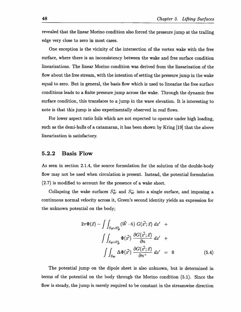
The agreement, however, of the integrated forces on the foil (figure 5-2) are not as
good as that of the pressure distribution at mid-chord. This, of course, is due to the
52 Chapter 5. Lifting Surfaces
.- ,2.0
1.5
C-II 1.0
analytic solution
0.0
-0.5
-1.0I I i I i i I I I I I
-0.5 -0.25 0 0.25 0.5X
Figure 5-1: The pressure distribution of a two-dimensional Karman-Trefftz sectionwith parameters xc = 0.1, Y, = 0.1, T = 10, at a 20 angle of attack.
fact that lifting line theory ignores any spanwise velocities and therefore the three-
dimensional method produces a different, presumably more correct, solution near the
tips. Prandtl's theory also assumes an elliptic distribution of circulation, which is
not exactly true for an elliptic planform. In fact, the geometry of the discretized foil
which was used was not precisely elliptic, due to wake paneling difficulties at the tip.
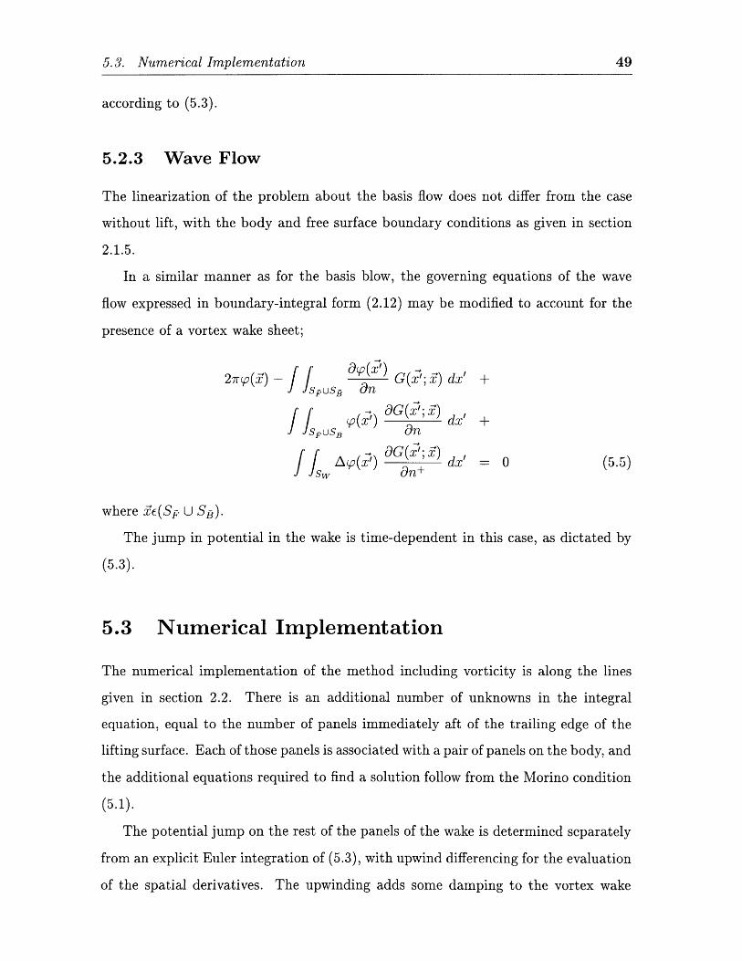
Considering all of the above, the results are promising and in addition demonstrate
that the solution is convergent and well behaved, even near the tip of the foil where
problems might be expected to arise in a potential flow numerical method. This can
also be seen in figure 5-3, which shows the spanwise distribution of the bound vorticity,
and the potential along several chordwise strips of panels on the body. There is no
numerical anomaly whatsoever near the tip.
A linearized, somewhat arbitrary wake geometry has been assumed in the above
investigation. This only approximates the position of the wake in the real flow. More
exact results could, in principle, be produced by tracing the wake at each time step
according to the fluid velocity induced at each point. Work has been done in this
5.4. Validation
(/ 1
M0.9Lt
o 0.8-jII 0.7
0.6
0.5
0.4
0.3
0.2
0.1
0
o 0.020
0-0.018
o 0.016
11 0.014
0.012
0.010
0.008
0.006
0.004
0.002
0.000
(b)-
-
-- - .-- -o- - - 0
30 40 50 60 70 80N (panels on both sides in chord)
Figure 5-2: The convergence of the lift (a) and drag (b) coefficients for an elliptical foilwith aspect ratio A = 10.19 and the section of figure 5-1, as computed by pressureand Trefftz plane integration. The analytic estimation is made by correcting thetwo-dimensional lift and drag coefficients along the foil using Prandtl's lifting linetheory.
0 2 4 6 8y (spanwise coordinate)
0.30
S0.25
0.20
0.15
0.10
0.05
0.00
--0.05-0.10
-0.15
-0).5 -0.25 0 0.25 0.5x (chordwise coordinate)
Figure 5-3: Demonstration of good numerical behavior at the tip of an elliptical foilwith A = 10.19. Shown, are the spanwise distribution of bound vorticity (a), andthe chordwise distribution of potential at several sections of the foil (b). The sectionused is as described in figure 5-1
Figure 5-4: Lift (a) and drag (b) sensitivity to the position of the wake. 0 = 0 impliesthat the wake is aligned with the free stream. The foil used has an elliptical planformwith A = 10.19 and the section shown in figure 5-1.
area for the unbounded fluid case [39], but it is beyond the scope of this study to
go to such detail. The extra computational effort required would render the present
method impractical for real applications, since the panel influence coefficients would
have to be re-evaluated at each time step.
Instead, in order to examine the importance of exactly specifying the wake loca-
tion, the sensitivity of the global forces to the position of the wake was investigated.
A plot of lift and drag coefficients versus the angle of the wake to the direction of the
free stream is shown in figure 5-4. It is evident that the global forces are not greatly
affected by the position of the wake, as long as it is within a few degrees of its true
position. This is especially true of the forces calculated by pressure integration. There
is, therefore, flexibility in the wake placement, a fact which is put to use in chapter
9, when numerical difficulties arise from the panelization of a complex geometry.
5.4.2 Surface Piercing Foil
The next step towards validating the lifting model, was to run the code for a surface
piercing hydrofoil and compare the results to prior experimental and numerical work.
The foil used for these tests had a rectangular planform with a span of 57 inches
and a chord of 161 inches. The section shape was symmetric, with a thickness-to-
5.4. Validation
chord ratio of T/C = 0.09. This particular foil was chosen due to the availability of the
PACT'95 syndicate's experimental data from their America's Cup testing program.
Runs were performed at a yaw angle of a = 20, over a range of speeds.
Observation of real flows just behind the trailing edge reveals that after a critical
Froude number, a sharp jump occurs in the free surface elevation across the wake
[3], [26]. This jump cannot be predicted by linear potential flow theory if both the
wake and free surface conditions are linearized about the free stream. In this case the
requirements of constant pressure across the wake and on the free surface would lead
to a zero jump in the free surface across the wake.
In the present method, however, the free surface conditions are linearized about a
basis flow, which also includes a jump in potential over the wake, A(I. The theoretical
elevation jump is therefore non-zero and given by
A( 1= + - V- = 2A(V(I " VI) + A(V( -Vp) (5.10)
In addition, the free surface is divided into two separate spline sheets, which have
a common boundary at the intersection with the wake sheet. There is no continuity
condition across these free surface sheets, and hence the wave elevation is free to have
a jump at this boundary without violating the assumptions of linear theory.
Figure 5-5 shows the wave pattern of the flow past the foil at Froude numbers of
0.3 and 1.0. The latter speed is beyond the critical Froude number and a jump in the
free surface elevation at the trailing edge may be observed.
The lift coefficient and the free surface jump as a function of Froude number are
shown in figure 5-6 and it can be seen that for this configuration, the critical Froude
number where the free surface elevation jump occurs is approximately 0.4. A sharp
increase in the lift coefficient occurs at this speed, followed by an apparent drop to a
high Froude number limiting value. Experiments were available for the higher speeds
shown, which agree well with the predictions of the numerical method.
The wave elevation near the trailing edge of the foil is further examined in figure
5-7, for Froude numbers ranging from 0.3 to 1.0. It can be seen that at the outset of
55
56 Chapter 5. Lifting Surfaces
Fn=0.3
Fn=1.0
Figure 5-5: Wave patterns of a surface piercing foil at F, = 0.3 and F, = 1.0
j 0.2 5
o
0.5 1.0 1.5 2.0 2.5U/(gL)
0
Figure 5-6: The lift coefficient (a) and the(b) as a function of Froude number, for a
jump in wave elevation at the trailing edgesurface piercing foil.
S0.10
0.09
u. 0.08
_ 0.07II
0.06
0.05
0.04
0.03
0.02
0.01
o.o%.
(a)
-D
- experimentsSWAN 2
. . . I , , , , I , , ,
iiilllllllll~''' .........
5.4. Validation
0.13
0.10
0.08
0.05
0.03
0.00
-0.02
-0.05
-0.07
-0.10
-0.12
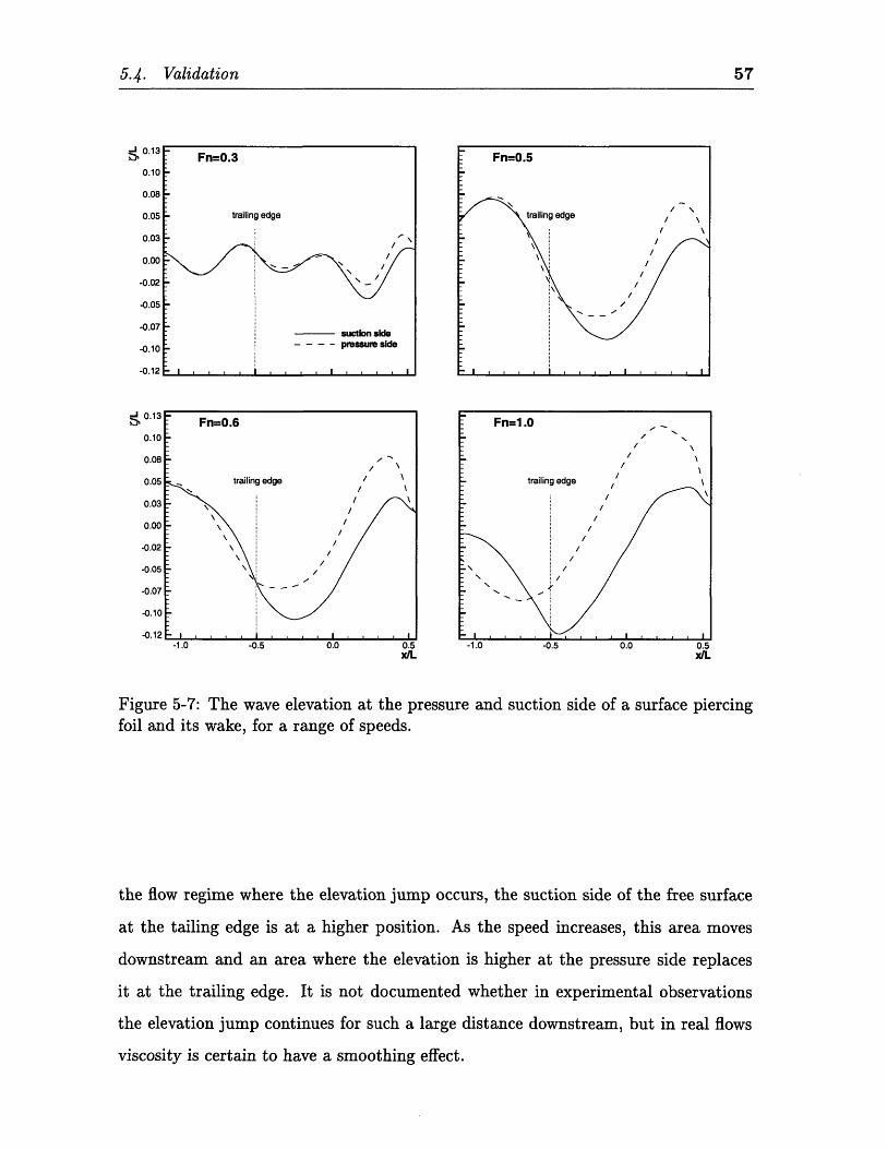
Figure 5-7: The wave elevation at the pressure and suction side of a surface piercingfoil and its wake, for a range of speeds.
the flow regime where the elevation jump occurs, the suction side of the free surface
at the tailing edge is at a higher position. As the speed increases, this area moves
downstream and an area where the elevation is higher at the pressure side replaces
it at the trailing edge. It is not documented whether in experimental observations
the elevation jump continues for such a large distance downstream, but in real flows
viscosity is certain to have a smoothing effect.
Fn=0.3
trailing edge
-/
-/
-
suction side- pressure side
- I II I i l r l i l l
Chapter 5. Lifting Surfaces
5.5 Conclusions
A linear three-dimensional time-domain Rankine panel method for the simultaneous
prediction of free surface waves, lift and induced drag has been developed. Both
steady and unsteady flows may be predicted, over a wide range of Froude numbers.
A linearized wake geometry was used, but the sensitivity of its actual position to
the lift and induced drag of the body was quite low.
The numerical method displays good convergence properties with an increasing
number of panels, and the agreement of the integrated forces with experiments for a
surface piercing foil was satisfactory. In addition, the wave pattern was accurately
resolved and shows a jump in the wave elevation at the trailing edge, as is observed
for real flows.
The method is therefore considered mature for application to real problems such
as sailing yachts and catamarans. Chapters 9 and 10 present results for such cases.
CHAPTER 6
THIN BODIES
The extension of the present Rankine Panel method to bodies with infinitesimally
small thickness was motivated by the fact that there are numerous marine appli-
cations, such as the sails on a yacht, the damping plates on an offshore platform,
and other appendages like rudders and winglets, which have a thickness very small
compared to the overall dimensions of the structure.
To discretize such bodies on both sides and use the existing formulation would
not only be inefficient from a computational efficiency point of view, but would also
encounter fundamental numerical difficulties due to the proximity of the Rankine
panel collocation points on the two surfaces of the thin body.
The solution is to treat the thin body as a single dipole sheet and re-formulate the
boundary value problem to obtain an integral equation for the unknown strength of
the dipole distribution. The problem is formulated in section 6.1 and the numerical
implementation is given in section 6.2. The method is validated with some examples
in section 6.3.
6.1 Formulation
Sections 2.1 and 5.2 have formulated the problem for bodies of finite thickness. An
extension to thin bodies follows.
The body is considered infinitesimally thin and is composed of two surfaces, SP+
and Sp, which occupy the same position but have opposite normal direction. As
with the case of the vortex wake (section 5.2), these two surfaces are combined into a
single jump surface Sp, which in the present method is represented by a dipole sheet.
Extending the notation of chapter 5, A is the operator which denotes the jump in a
quantity across the thin body, and the superscripts "+" and "-" denote quantities
on the surfaces S + and Sp, respectively.
If the thin body produces lift, the trailing vortex wake Sw, is treated exactly as
described in chapter 5.
The usual boundary conditions, as described in section 2.1.3, apply in the presence
of a free surface SF, or a "thick" body SB. For a thin body, the body boundary
conditions become
+ an+ W n(6.1)On+ On+
By applying Green's second identity, collapsing the dipole sheets into single sur-
faces, and making use of the boundary conditions, the following integral equation is
obtained;
- f( () aG(X; 9) dx' +
II u sG('; YIG(S; Y) -27r(IF) + I()-) (SSp U Sw)
pUSw an+ -21-(Y) . /(Sp U Sw)
The RHS of (6.2) is different when the point Y is on a dipole sheet because there
is fluid on both sides of the singularity. In this case, the above equation cannot
be used to determine the potential jump on Sp because two extra unknowns, 1@+
and *-, have been introduced. Instead, the normal derivative of equation (6.2) is
taken for points on Sp, and the body boundary condition (6.1) is used to eliminate
the normal derivatives of the potential. A new boundary integral equation is hence
obtained, which may be coupled with (6.2) for points on Sa or Sp in order to solve
60 Chapter 6. Thin Bodies
6.2. Numerical Implementation 61
the complete problem;
I S '(5t) OG(x';Y) dx' +spus, n Op
- 02 G( ; Y) dx' =f spuswOpOn
I ISPuSBA(X-) ap dxn+ =x -2w (O ) -
-4(W + -) -P (6.3)
where ' is the unit normal to St at point F.
After the boundary value problem has been solved, the actual value of the potential
on the thin body may be found by using equation (6.2), combined with the definition
of the potential jump. This is necessary if the fluid velocities on the two sides of the
thin body are to be determined.
6.2 Numerical Implementation
The base of the numerical algorithm is identical to that for a thick body, presented
in sections 2.2 and 5.3.
After discretization, (6.3) gives one equation per panel on the thin surface, to
determine the unknown jump in potential. In addition, one equation per panel for
the other surfaces is produced by (6.2). Double derivatives of the Rankine source
potential are required in order to obtain the coefficients of the new integral equation
(6.3). These are automatically computed by the same algorithms [35] that are used
for the evaluation of the coefficients of the original integral equation (6.2).
For lifting surfaces, constant panels with cosine spacing at the leading edge were
needed for a non-oscillatory solution, similar to what was found for thick bodies in
section 5.
It must be mentioned that the available subroutines for the evaluation of the
influence coefficients do not calculate the velocity induced at a field point due to a
distribution of normal dipoles of quadratic strength over a planar quadrilateral panel.
Therefore, the second term of the LHS of equation (6.3) cannot be readily evaluated
on Sp using the existing software. This can be easily addressed in the future, but
for the purpose of this work the above term was evaluated assuming an equivalent
distribution of constant strength on each panel of the bi-quadratic spline sheet on the
body or the free surface. This does not cause significant errors unless the panels of
the dipole sheet are too close to the bi-quadratic spline sheet, as shown in section 6.3.
6.3 Validation
Some results are presented in this section, both in an infinite fluid and in the presence
of a free surface, in order to validate the implementation of the method.
6.3.1 Foil in Unbounded Fluid
An obvious first check to validate the method for thin bodies, is to determine how
close the solution for a thin plate approaches to the limit of a foil of finite thickness
of the same planform.
This test was indeed performed for a cambered foil of aspect ratio A = 0.5, and
the results are shown in figure 6-1. The lift coefficient as a function of the thickness-
to-chordlength ratio is shown along with the distribution of the potential jump over
the chordlength of the plate at mid-span.
As expected, the numerical method has encounters difficulties when the two sur-
faces of the body are too close to each other. In this case, the proximity of the
distribution of singularities on the two surfaces causes the influence coefficients in the
boundary integral equation to be of very large magnitude. The numerical scheme tries
to find a solution by subtracting large quantities, and after a point which depends on
the accuracy of the particular machine on which the code is running, it fails.
But when the thin body is treated as a dipole sheet, no more such numerical
problems are encountered and it can be seen that the value obtained in this case
is clearly the low thickness-to-chordlength ratio limit of the "thick-body" method,
before it fails.
62 Chapter 6. Thin Bodies
6.3. Validation 63
0.40
0.35 0.1(b)
0.30 < 0.10
0.25 0.05
0.20 0.00 -
0.15 ..... .................. plate---- l -0.50 -0.25 0.00 0.25 0.50
0.10 x/C
0.05
0.00 . I ......10 10 10. 10
"
t/c
Figure 6-1: The lift coefficient of a rectangular planform foil with A = 0.5 as afunction of thickness-to-chordlength ratio (a), and the distribution of the potentialjump over the chordlength of the plate at mid-span (b).
6.3.2 Submerged Horizontal Plate in Heave
A second test to validate the method for the unsteady problem was to analyze the
flow associated with a heaving horizontal plate submerged under the free surface.
The plate taken for this study was circular with diameter d, and was submerged at a
depth equal to one radius under the z = 0 plane.
The heave added mass of a body in an unbounded fluid is given by
M = p p dS (6.4)
where 'p is the radiation potential of the body in heave [34].
For a thin plate where the surface SB is collapsed into a jump surface Sp (see
section 6.1), and for a unit translation velocity, the above condition becomes
ma3 = p jff A1 p dS (6.5)
The added mass may be, therefore, easily computed numerically using the present
Rankine panel method to solve the infinite fluid problem for the plate translating
Chapter 6. Thin Bodies
4U
39 (a) theoretical value(a- --- SWAN 2
38
37
36
35
34
33
32
31
301 I I I I10 20 30 40
N [panels azimuthally]
(b)0.15
0.10
0.05
-0.05
-2 -1 0 1 2x/d
Figure 6-2: Heaving circular plate. (a) The convergence of the heave added massin an unbounded fluid and comparison with theory. (b) The wave elevation abovethe plate heaving with amplitude A, one radius (d/2) below the free surface. Thefrequency of heave is w = 1.5(g/d)1/2
with a steady unit velocity, and then directly evaluating (6.5).
The analytical solution for the above problem has been given by Lamb [21];
1dm33 =P 3
3(6.6)
The convergence of the method for an increasing number of panels on the circular
disk is presented in figure 6-2(a) along with the theoretical value (6.6). The results
are clearly convergent, and agree well with theory.
Adding a free surface to the problem, the wave pattern for the plate heaving at a
normalized angular frequency (w /g) of 1.5 radians is shown in figure 6-2(b).
The added mass and damping of the plate heaving at a depth of one radius
below the free surface may be calculated from the radiation potential by direct linear
pressure integration. But the damping may also be found from the excitation force in
the diffraction problem. More specifically, the Haskind relations [34] may be used to
show that the heave damping coefficient of a body with a vertical axis of symmetry
64
> 0.40 0.10
C 0.39 0.09
0.38 ~ 0.08 -
0.37 0.07
0.36 0.06
0.35 0.05 / radiation- - - - Haskind
0.34 0.04
0.33 7 0.03 /
0.32 0.02
0.31 0.010 - 1.5i I . . . LI . . . . 0.I
0.
3.0 1.25 1.50 1.75 2.00 .
0 0 1.25 1.50 1.75 2.00
(o (d/g) co(d/g)
Figure 6-3: The heave added mass (a) and damping (b) of a horizontal circularplate submerged at a depth of one radius. The damping is calculated from both theradiation and diffraction problems.
is equal to
b33 = X312 (6.7)2pg
where IX3 1 is the vertical excitation force in regular waves of unit amplitude.
The added mass of the circular disk is presented in figure 6-3(a) as a function of
frequency. The heave damping of the plate as found by both the above methods is
in good agreement, as shown in figure 6-3(b), suggesting that the thin-body method
gives plausible results for both the radiation and diffraction problems. The slight
disagreement at low frequencies is due to the fact that, in order to obtain a domain size
large enough to accommodate the wavelengths involved, a coarser grid with respect
to the dimensions of the plate was used on the free surface in this case. As explained
in section 6.2, the method as currently implemented can introduce errors when the
dipole sheet is at a depth smaller than the order of magnitude of the dimensions of
the free surface panels.
6.4 Conclusions
A linear three-dimensional time-domain Rankine panel method has been extended
to include bodies of infinitesimally small thickness. Both steady and unsteady flows
6.4. Conclusions 65
66 Chapter 6. Thin Bodies
may be predicted in the presence of a free surface or in an unbounded fluid.
The numerical method displays good convergence properties with an increasing
number of panels, and the solution has been demonstrated to approach the limit of
the method for bodies with decreasing but finite thickness.
Real problems, such as the flow past the sails of a sailboat, may now be tackled.
Chapter 9 presents results for such a case.
Care must be taken when thin bodies are close to surfaces which are described
in terms of bi-quadratic spline sheets, as the method currently approximates the
influence of a quadratic distribution of normal dipoles on panels of such sheets with
an equivalent constant dipole distribution.
CHAPTER 7
DEEP TRANSOM STERNS
A vessel with a deep transom stern is defined as one with a truncated afterbody,
ending in a flat vertical section below the still waterline (figure 7-1). Since the great
majority of modern ships have a stern of this type, it is imperative to be able to
accurately model the flow in this region.
This chapter presents a method of resolving the numerical difficulties associated
with the flow past a transom stern. The problem is formulated in section 7.1 and the
numerical implementation is discussed in section 7.2. Some results are presented in
section 7.3 for validation, while conclusions are drawn in section 7.4.
7.1 Formulation
For ships with transom sterns, the formulation of the problem as presented in section
2.1 is not complete. Since the flow separation at the sharp lower edge of the transom
is triggered by viscous effects, the correct behavior must be explicitly enforced in the
present potential flow mathematical model.
The real flow past a transom stern can exist in any one of three different regimes.
The first regime occurs at low speeds or deeply immersed transoms, and is character-
ized by a stagnation pressure at the stern. In this case the transom remains wet and
the viscous effects are dominant in the region.
Chapter 7. Deep Transom Sterns
Figure 7-1: Profile view of a typical deep transom stern
The second regime occurs as speed is increased or the transom immersion is re-
duced. The flow detaches at the sharp transom edge and the transom itself remains
dry. According to a rule of thumb [42], transition from the first regime to this type
of flow often occurs at transom Froude numbers
UFT = 4.0 (7.1)
where ZT is the depth of immersion of the transom at zero speed. Most high-speed
ships operate in this regime.
Finally, as transom immersion is further reduced so that the lower edge lies above
the undisturbed free surface, the flow detaches at some point at the bottom of the
hull before reaching the stern. Sailing yachts, for example, are very often designed to
operate in this regime.
The first regime cannot be accurately modeled using a potential flow method
and is, therefore, outside the scope of this study. In any event, such a flow is very
inefficient, needs to be avoided by the ship designer, and thus rarely needs to be
analyzed.
The third regime is highly non-linear, and cannot be predicted by the present
linear method. A linear method can hope to achieve some approximate modeling of
the flow by assuming, for example, that it detaches at the intersection of the body
with the linearized free surface and by treating the flow as if it were in the second
regime.
The present work will concentrate on transom flows in the second regime, where
the line of detachment is well defined, as shown in figure 7-1.
The free surface just aft of the transom must obey the dynamic and kinematic
free surface conditions, and the mixed boundary-integral equation, just as at any
other point on the free surface. But in order to enforce a flow detachment it may be
necessary to impose some additional continuity conditions at that point.
* The wave elevation (T, should be equal to the instantaneous transom depth zT.
(T = ZT (7.2)
* Due to the smoothness of the solution, the wave slope at the transom may be
imposed to be equal to the slope of the hull. The lack of this condition would
allow a corner flow at the transom edge.
8T OZTS ZT (7.3)Dx Ozx
S- OZT (7.4)Dy Oy
* At the transom, the velocity potential 9T, and/or its normal derivative ,
should be equal on the body and in the free surface wake.
7.2 Numerical Implementation
As seen in the previous section, it is necessary to impose extra conditions at the
free surface panels immediately downstream of the transom. By incorporating both
the free surface boundary conditions and the continuity requirements at the stern,
however, the problem becomes over-specified.
7.2. Numerical Implementation 69
Chapter 7. Deep Transom Sterns
7.2.1 Transom Conditions
The linearized kinematic boundary condition for a given wave elevation and slope
provides an expression for the normal velocity at the linearized free surface, z = 0.
099_ 5(T a2_- - ( - V4) . VT - Oz2 (7.5)
This, however, is in conflict with the solution of the mixed boundary-value prob-
lem. Recall that the same value 2, is calculated on the entire free surface by solving
the boundary-integral equation (2.12). In general, the value obtained by Green's
identity does not satisfy (7.5) at the stern.
Similarly, the dynamic free surface boundary condition just aft of the stern can
be used to determine the value of the potential on the linearized free surface.
at ( - V(P) "Vp = -gT + V - - V1 1 I V( ID (7.6)
But for a two-dimensional transom flow, Schmidt [43] used a flat-ship linearization
to show that the curvature of the free surface has a square-root singularity at the
transom. The bi-quadratic spline functions which are used by the present numerical
method to represent the unknowns on the free surface, cannot accommodate the
infinite curvature which is necessary to impose zero pressure at the stern. This leads
to numerical difficulties, as a solution cannot be found which satisfies (7.6) for a
specified wave elevation.
The above difficulties are mainly due to the fact that the transom conditions are
basically inconsistent with the free surface linearization. Linear theory assumes that
the variation of the hull shape near the waterline is small. Then, the exact position
of the intersection of the hull with the free surface has a negligible effect on the flow.
But for transom flows, where the hull curvature is infinite and a particular line of
detachment is desired, the above assumptions are not valid. Raven [40] found that
by adopting a fully non-linear treatment of the boundary conditions for the steady
flow problem, the difficulties disappeared.
7.2. Numerical Implementation 71
For the present implementation, there is a choice of the condition used to specify
each of the three unknowns - wave elevation, potential, and normal velocity - at
the free surface immediately aft of the transom. Each one may be specified by using
three alternatives; continuity from the hull, a free surface boundary condition, or
Green's second identity. A study was carried out to determine a combination which
gave both convergent and physically plausible results.
It was concluded that the best implementation of the transom conditions was
to specify the wave elevation according to (7.2), the potential by continuity from the
hull, and the normal velocity through the solution of the boundary-integral equations.
The wave slope was not explicitly specified according to (7.3) and (7.4) but it was
found to have a realistic behavior for the practical calculations which were performed.
Even if the free surface slope had been imposed, however, it would have been diffi-
cult to exactly simulate the physical behavior of the flow using bi-quadratic spline
functions, because of the theoretically infinite curvature at the trailing edge.
The same approach was used for the dynamic boundary condition. Equation (7.6)
was not directly enforced, but in practice the resulting non-zero pressure at the stern
was found to have a very localized effect.
7.2.2 Local Flow
An additional numerical difficulty was encountered for the present time-domain method
due to the division of the perturbation potential into local and memory flows. The
local flow, which is the pressure release problem (<p = 0 on the free surface), separates
the local added mass from the forcing in the equations of motion. The motivation
for this stems from numerical stability considerations, as shown by Kring [18]. For
transom flows, however, the sharp corner at the lower edge of the transom becomes
the source of high velocities in the local flow, which affect the total solution.
This problem was solved by paneling the transom with a spline-sheet of specified
potential and solving for the normal velocity using the boundary-integral equations.
The value of the potential in the interior of the transom surface is interpolated from
the hull panels at the edge of the transom. This leads to a slowly varying distribution
Chapter 7. Deep Transom Sterns
body plan
waterlines plan
sheer plan
Figure 7-2: The lines drawing of the test transom-stern ship used in this study. Onlythe underwater portion of the hull is shown.
of potential on the transom, which ensures that the major component of velocity is in
the normal direction, into the fluid. The large velocities from the corner in the local
flow are hence eliminated and a smooth solution is obtained.
7.3 Validation
The above implementation was validated using a simple test hull, the lines of which are
shown in figure 7-2. This hull has a deep transom, beam to length ratio BIL = 0.1,
and draft to length ratio T/L = 0.0625. The maximum depth of the transom is
1.25% of the length of the hull. The solution was obtained at a hull Froude number
of F, = 0.4 which is equivalent to a transom depth Froude number of F., ; 3.56.
The convergence of the wave patterns and pressure distribution on the hull was
investigated for an increasing number of panels. Figure 7-3 shows the results of this
convergence study for the steady flow problem, where some contour plots of the wave
elevation and the pressure distribution on the hull are presented for an increasing
number of panels.
The same quantities are displayed in figure 7-4, where a comparison is made
___
7.3. Validation
30x8 panels on body
40x10 panels on body
50x12 panels on body
Figure 7-3: Contour plots of the wave elevation and pressure distribution on atransom-stern hull, for an increasing number of panels.
74 Chapter 7. Deep Transom Sterns
F0.015'>10
._ 0.01a
0.005-0.005
0.005
-0.01
-0.015
-0.015
00.0
- 0.01
-0.01
-0.015
-1
transom : x/L=-0.5 x/L
-0.5 0x/L
Figure 7-4: A comparison between the present time-domain method (a) and an equiv-alent frequency-domain method (b) for the steady flow solution past a transom-sternhull.
Figure 7-5: The heave (a) and pitch (b) RAO of a transom-stern ship. Conver-gence with an increasing number of panels and comparison with a frequency-domainmethod.
between the steady solutions of the present time-domain method and an equivalent
frequency domain method (SWAN 1). It must be noted that the frequency-domain
method employs a different set of transom conditions, which causes the dynamic
pressure at the transom edge to come closer to balancing the hydrostatic pressure,
as theoretically required. Due to stability problems, it was not possible to employ
these same conditions in the time-domain. The aforementioned conditions which were
employed, however, result in a wave pattern and pressure distribution almost identical
to the frequency-domain method, with the exception of the body in the immediate
vicinity of the transom. As expected, however, this effect is localized and does not
affect the global solution. It can also be argued that the time-domain solution is
closer to the physical solution due to the singularity at the transom edge. The present
method eliminates the singularity in the formulation of the transom conditions and
thus obtains a smooth solution. The frequency-domain method, however, attempts
to capture the exact value of the pressure at the stern but the spline functions cannot
resolve the singular behavior of the flow in the area, thus possibly resulting in a
pressure drop over a larger area of the hull than what occurs in reality. Experiments
were not available to support or deny this argument.
Chapter 7. Deep Transom Sterns
The problem of motions in waves was examined next, and figure 7-5 displays the
convergence of the heave and pitch Response Amplitude Operators with an increasing
number of panels. A comparison with the frequency domain method is also shown
in the same figure. After resolving the numerical difficulties in the local flow, the
convergence of the method is excellent. The agreement with the frequency-domain
method is fair, with the differences again being due to the different transom conditions
employed by the two methods. As will be presented in chapter 10, experimental data
suggest that the motions as predicted by the current time-domain method are more
accurate.
7.4 Conclusions
A robust, convergent method has been developed, which is capable of predicting the
flow past deep transom sterns. This problem was previously unsolved in the time-
domain, because of numerical difficulties. These difficulties have been resolved by
paneling of the "dry" portion of the stern, which had a smoothing effect on the local
flow, and by choosing appropriate transom conditions.
It must be noted that although the present method presents satisfactory results
it does not model the precise behavior of the flow at the transom edge. The local
effect of infinite curvature leading to zero pressure at the stern is not captured by
this linear method. In fact, the real flow near the transom is not very suitable for
linearization. Fortunately this is a very local anomaly, similar to the spray near the
bow, for example. The transom conditions which have been employed eliminate the
singularity at the stern, thus producing a solution which is believed to be closer to
the actual flow than what is obtained when the exact value of pressure is enforced at
the transom.
The method is intended for flows which separate exactly at the transom edge.
While this accurately models the flow behavior for most vessels with such sterns,
there are some cases where it is not applicable. The flow past the transoms of IACC
sailing yachts is one such non-linear example which will be examined in more detail
7.4. Conclusions
in chapter 9.
77
78 Chapter 7. Deep Transom Sterns
Part IIIApplications
1992 America's Cup Defender Trials
CHAPTER 8
CONVENTIONAL SHIPS
This chapter presents some applications of the numerical method to conventional
ships. Since more experimental data exist for such vessels than for advanced marine
vehicles, these cases serve as validation of the method in order to gain more confidence
when examining more complex cases.
The wave patterns are checked for convergence and are compared to experiments
for two characteristic hulls. Section 8.1 presents results for a single-screw merchant
ship, the Series 60 (CB = 0.7). A modern naval ship, model 5415, is examined in
section 8.2.
8.1 Series 60
The lines drawing of the Series 60 hull which is examined in this section is shown in
figure 8-1. All the results presented below are for a Froude number F, = 0.316.
When analyzing the flow past a ship, it is important to have confidence that the
numerical solution is not affected by the truncation of the free surface. Figure 8-2
provides proof that the for a sufficiently large domain size, the wave pattern near the
ship is virtually unaffected. The wave patterns for the two domain sizes shown differ
only near the edges, where the effect of the damping zones becomes significant.
Figure 8-3 presents some contour plots of the wave elevation on the free surface
Conventional Ships
body plan
waterlines plan
sheer plan
Figure 8-1: The lines drawing of the Series 60.
Figure 8-2: Domain sensitivity for the Series 60.
Chapter 8.
8.1. Series 60 83
1752 panels
2860 panels
3914 panels
Figure 8-3: Contour plots for the wave elevation and pressure distribution on theSeries 60 hull, at Froude number 0.316, for an increasing number of panels.
84 Chapter 8. Conventional Ships
0.020
30 panels along waterline (a) 0.0120 - -- 30 panels along waterline (b)0.015 40 panels along waterline ---- .40 panels along waterline
50 panels along waterline 50 panels along waterline
Figure 8-4: The wave profile along the hull (a) and the wave heights at a cut alongy/L=0.108 (b) for the Series 60 hull at Froude number 0.316. Results are shown foran increasing number of panels and are compared to experiments.
and the pressure on the body, with an increasing number of panels. The solution
seems to converge, and this may be observed more easily from the plots of the wave
profile along the hull and along a longitudinal cut at y/L = 0.108, as shown in
figure 8-4. The numerical results not only are convergent, but also agree very closely
with experiments. The slight differences, which are most noticeable immediately
downstream of the stern, are attributed to viscous and other non-linear effects which
are not modeled by the present method.
8.2 Model 5415
With a sonar dome and a deep transom stern, Model 5415 represents a naval combat
ship with a considerably more complex form than the Series 60, examined above. The
lines for this hull are shown in figure 8-5.
Experimental data were available for this hull at a Froude number of F, = 0.2755.
At this speed, the transom depth Froude number as defined by (7.1) is equal to 3.8,
and hence flow separation is most likely to occur at the stern.
Although the wave profile along the hull and along a cut at y/L = 0.097 show
8.2. Model 5415
body plan
waterlines plan
sheer plan
Figure 8-5: The lines drawing of Model 5415.
0.008
0.004
0.000
-0.004
-0.008
-1.50 -1.00 -0.50 0.00 0.50 1.00x/L
Figure 8-6:y/L=O.097
The wave profile along the hull (a) and the wave heights at a cut along(b) for Model 5415 at Froude number 0.2755. Results are shown for an
increasing number of panels and are compared to experiments.
--------- 30 panels along waterline (b)----------
40 panels along waterline
- 50 panels along waterline.............. experiments
~I * l ~ I t l I I I I l l l I l I
x/L
_ __ ~_
86 Chapter 8. Conventional Ships
. 0.04 . 0.020
30 panels along waterline (a) --------- 30 panels alongwaterline (b)40 panels along waterline 0.016 --------- 40 panels along waterline
0.03 - 50 panels along waterline - 50 panels along waterlineexperiments 0.012
Figure 8-7: The wave profile along the hull (a) and the wave heights at a cut alongy/L=0.097 (b) for Model 5415 at Froude number 0.4136. Results are shown for anincreasing number of panels and are compared to experiments.
convergence with an increasing number of panels (figure 8-6), the agreement with
experiments is not as good as for the Series 60. This fact is attributed to the non-
linearities associated with the sonar dome and the deep transom stern, which were
not present in the more linear Series 60 hull. Nevertheless, the agreement is still as
satisfactory as can be expected of a linear panel method.
The convergence is also slower relative to what was observed for the Series 60 hull.
Lower speeds combined with the presence of a transom flow are known to produce
wave patterns dominated by shorter wavelengths, which require a greater number of
panels to be fully resolved.
Convergence properties improve as the Froude number increases, as can be ob-
served from figure 8-7, where the wave profile along the hull and along a longitudinal
cut at y/L = 0.097 are shown for a Froude number F, = 0.4136.
Even though the wave patterns for the higher Froude number converge faster,
however, an area still seems to exist, aft of the deep transom stern, where rate of
convergence is not as fast as would be desired. The reason for this poor behavior is
due the inconsistency with linear theory of the physical flow at the outer corner of
the transom. The error propagates out and aft with the flow, following the diverging
8.2. Model 5415 87
wave pattern of the ship.
It is, however, very encouraging to note that in all cases the convergence of the
wave profile on the hull is excellent. This is an indication that the integrated forces
are also convergent. Quantities such as wave elevation and pressure are only used
over the surface of the hull for the evaluation of the wave forces.
88 Chapter 8. Conventional Ships
CHAPTER 9
SAILING YACHTS
This chapter presents a complete case study involving the IACC sailing yacht shown
in figure 9-1. Sailing vessels have complex hulls and many of the extensions provided
in this thesis have been used to carry out the analysis. In fact, most of the extensions
were actually motivated by the study of sailing yachts.
Due to the proper treatment of the keel and rudder as lifting surfaces (chapter 5),
the panel method is used to predict the interaction of those appendages with the
free surface. The validity of the existing practice of treating the keel and rudder
independently of the free surface flow is thus examined.
The flow near the transom of the vessel is especially complex, and requires the
numerical approach developed in chapter 7. The steady resistance is hence estimated
and an approximate method to treat the non-linearities in this area is devised.
Finally, a full time-domain simulation is performed by modeling the flow in air
and in water simultaneously. The sails are treated according to the thin body theory
developed in chapter 6 and the aerodynamic forces are coupled with the hydrodynamic
forces through the equations of motion. It is therefore possible to investigate the
effect of the added mass and damping of the sails as the vessel pitches and rolls. This
coupled approach in the time domain allows the assessment of the forces on the rig
in irregular seas, even with the future inclusion of non-linear effects in the code.
90 Chapter 9. Sailing Yachts
body plan
waterlines plan
sheer plan
Figure 9-1: The lines drawing of an IACC yacht.
9.1. Gridding Issues
9.1 Gridding Issues
9.1.1 Asymmetry
The most striking visual difference of the underwater portion of a sailboat hull from
a conventional ship is the presence of a fin-keel, which generates lift to balance the
aerodynamic side-force from the sails. With the exception of any trim tabs, this
keel is port-and-starboard symmetric and, therefore, the yacht needs to sail under
a mean leeway angle in order to produce the required amount of lift. In addition,
sailing yachts usually travel under heel in order to provide static righting moment
to balance the dynamic heeling moment of the rig and keel. This presence of heel
and yaw eliminates the usual advantage of using symmetry to panel only half of the
domain, since the hull becomes asymmetric with respect to the mean flow direction.
The need to panel the whole domain, coupled with the presence of additional pan-
els due to the appendages and possibly even the sails, places unusually high demands
on computing power.
The solution was provided by the use of a polar grid on the free surface, which
uses considerably less panels than a standard rectangular grid for the same resolution
near the body. Such a paneling scheme is also a natural fit for the rounded transoms
at the waterline that many sailing yachts possess. As an illustration, the polar and
the equivalent rectangular grids presented in figure 9-2 may be compared.
9.1.2 Appendages
Section 5.4 has presented some results involving lift of simple bodies. When a more
complex geometry such as the combination of a hull and a keel is considered, there
are some additional issues that need to be resolved.
One problem is that when the keel is modeled as a lifting surface but the rest of
the hull is not, then a tip vortex forms at the intersection of the two bodies, inducing
large velocities on the hull. This leads to numerical difficulties. In reality, of course,
the sectional lift coefficient does not fall to zero at that intersection, since the hull
92 Chapter 9. Sailing Yachts
polar grid45x11 panels on body2185 panels on free surface
rectangular grid45x11 panels on body5679 panels on free surface
Figure 9-2: A comparison of polar and rectangular free surface gridding.
9.1. Griddirig Issues 93
Figure 9-3: The discretization of the hull and keel of an IACC yacht.
also produces a small amount of lift. The numerical solution is to extend the keel up
inside the body to the z = 0 plane. The wake is then extended to pass through the
hull and ceases to cause numerical problems. Normal boundary and Kutta conditions
are applied to the internal portion of the lifting surface, but such panels are ignored
during pressure integration for force calculations. An analogous situation occurs at
the intersection of the fin-keel with the bulb.
The need to extend the wake through the hull eliminates some freedom of the hull
discretization. It is now necessary to have a cut in the hull spline sheet so that the
wake panels do not pass through any hull panels. The simplest way to accomplish this
is to discretize the hull in two sheets along the line of port-and-starboard symmetry.
Then, however, the wake needs to be aligned with the plane of symmetry of the vessel
and not with direction of the free stream flow. Fortunately, as shown in section 5.4,
the numerical method is not sensitive to small variations in the direction of the wake.
9.1. Gridding Issues 93
94 Chapter 9. Sailing Yachts
(a) Pressure integration + waterline term (b) Pressure integration0.0045 U,-
Figure 9-4: The resistance coefficient of an IACC yacht. Convergence of the numericalresults using pressure integration together with the waterline integral (a) and usingsimple pressure integration (b). The results by the approximate non-linear methodare also shown in (b). The coefficient is based on the surface of the hull below thez = 0 plane.
Figure 9-3 shows the resulting discretization of the hull and keel configuration which
was tested.
9.2 The Steady Resistance Problem
9.2.1 A Non-Linear Extension
Chapter 3 has described a method of resistance calculation which is used in conjunc-
tion with the present linear method to account for the dynamic wetted area of the hull
(3.6). This involves the evaluation of a waterline integral in addition to the pressure
integration over the hull below the z = 0 plane. Strong hull non-linearities, however,
are not expected to be fully captured by this method.
Sailing yachts commonly have hulls with significant flare and overhang at the bow
and stern. This causes the shape of the under-water portion of the hull to change
considerably with speed. But even with the highly non-linear hull of figure 9-1, the
numerical results converge to a resistance curve relatively close to the experiments
(figure 9-4(a)).
In some cases, however, a better degree of accuracy is desired, which is beyond the
capabilities of a linear method. Recently, fully non-linear panel methods have started
to become practical [40] - even if only for the steady resistance problem - but they
still require considerable computational effort. An approximate non-linear extension
to the present linear method was therefore developed, with the hope of capturing
the non-linearities associated with the dynamic wetted surface, without significantly
increasing the computational intensity.
The method consists of performing an initial run in order to find the intersection
of the hull with the free surface. The shape of the dynamic wetted surface of the
hull is then estimated, taking into account any sinkage and trim. A new hull-form is
then produced by vertically shifting each section so that the intersection with the free
surface moves to the z = 0 plane. A new run is performed with this modified hull.
The wave resistance is calculated by integration of the normal pressure force, using
the normal vectors of the original hull at any given x-y position. The force is then
scaled according to the ratio of the displacement of the original to the "stretched"
hull. This is necessary because, in general, the displacement of the modified hull is
found to be greater than that of the original one, a phenomenon which does not occur
in reality since the vessel has a fixed weight.
This author recognizes the crude engineering nature of the above approach to this
problem. No further attempt will, therefore, be made to justify the theoretical basis
of the method, other than to note its exceptional agreement with the experimental
results, shown in figure 9-4(b). The simple pressure integration consistently over-
predicts the wave resistance of the vessel. The subtraction of the waterline term
(3.6) brings the curve closer to experiments, but seems to miss the exact trend at
low speeds. As expected, the non-linear approach has the same general effect as the
waterline term, but is much more accurate. The difference with experiments at the
high end of the speed range is due to non-linearities in the free surface condition,
which are not modeled in either method.
9.2. The Steady Resistance Problem 95
96 Chapter 9. Sailing Yachts
without keel with keel
Figure 9-5: Contour plots of the wave elevation and body pressure for an IACC yachtwith and without the keel and bulb in place.
9.2.2 Appendage-Free Surface Interaction
When testing sailboat appendage configurations, usually in wind tunnel facilities,
it is common to ignore the effect of the free surface. The justification is that the
appendages are far enough immersed that the free surface may be treated as a rigid
wall. Conversely, hulls are often tested in towing tanks without the proper appendages
in place, assuming that their effect can be considered separately.
The numerical tool that has been developed, now enables the simultaneous study
of the hull, the keel, and the free surface. Figure 9-5, for example, compares the free
surface elevation and the pressure on the body for the hull with and without the keel
in place. It can be easily seen that the presence of the keel strongly affects the flow
near the free surface, especially on the windward side (right side as shown in figure
9-5) of the yacht. Reciprocally, the free surface is expected to affect the flow near the
keel. This interaction suggests that caution needs to be exercised before isolating the
appendages from the hull for experimental and numerical analysis.
9.3. Free Motion Simulations in Waves 97
1.5 .- 400
1.4 (a) (b)1.3 . < 350 m
1.2 -
1.1 ' 300
1.00.9 250
0.8200
0.7
0.6 O1500.5
0.4 0- experiments 1000.3 SWAN 2, 1591 panels
SWAN 2, 2518 panels0.2 SWAN 2, 3089 panels 50 - L
0.1 SWAN 1 0
0.0 0 J10 .0 1.5 2.0 2.5 0.5 1.0 1.5 2.0 2.5
X/L X/L
Figure 9-6: The Heave (a) and Pitch (b) RAO for an IACC hull traveling at Froudenumber 0.347 in head waves.
9.3 Free Motion Simulations in Waves
9.3.1 Head Seas
The prediction of the seakeeping performance of a vessel can be just as important
as the problem of steady translation. Experiments were available from the PACT'95
model testing program for the motions of the IACC yacht of figure 9-1. It was, there-
fore, possible to validate the enhancements to the method which have been developed
as part of this thesis, as applied to the particular geometric complexities of this IACC
hull. The above hull features a rounded transom stern which is characterized by a
slightly different flow behavior than the deep transom case which was examined in
chapter 7. Nevertheless, as can be seen in figure 9-6, the heave and pitch response
amplitude operators are clearly convergent with an increasing number of panels.
Figure 9-6 also presents a comparison of the experimental versus the numerical
response amplitude operators. Results using the frequency domain method, SWAN 1,
are also shown in the same figure. Satisfactory agreement with experiments is ob-
served. In fact, the present time domain method appears to be a slight improvement
over the frequency domain method.
9.3. Free Motion Simulations in Waves 97
98 Chapter 9. Sailing Yachts
9.3.2 Appendage Modeling
In addition to the steady motion case examined in section 9.2.2, the sailboat keel
and rudder are also expected to affect the problem in the presence of waves. This is
especially true for the transverse modes of motion. The present section examines the
importance of accurately modeling such appendages, as opposed to treating them in
an approximate fashion using lifting line theory.
The response amplitude operators were obtained for the vessel of figure 9-1 in bow
seas, at an angle of incidence equal to 45 degrees from the beam. A mean heel and
leeway angle were imposed in order to simulate actual sailing conditions.
In an attempt to capture the effect of the presence of the fin-keel, this component
was first entirely omitted, but the bulb was taken into account by placing panels on
its surface.
The fin-keel was then modeled by lifting line theory, ignoring its hydrodynamic
effect on the rest of the flow. The keel lift force, which was used to modify the
equations of motion, was computed according to its area, aspect ratio, speed, and
angle of attack. The apparent angle of attack was adjusted according to the motions
of the vessel and the incident flow velocity.
The RAOs obtained for the above appendage models were compared with the more
accurate method for treating lifting surfaces which has been developed in chapter 5.
The keel and bulb were paneled, and a trailing vortex sheet was added, as shown in
figure 9-3.
Due to computing power constraints, the effect of the rudder was taken into ac-
count using the approximate lifting line model as described above for the keel.
Figure 9-7 presents the effect of the fin-keel on the heave, pitch, roll, and yaw
motions of the sailing yacht in bow seas. It is immediately obvious that the presence
of the keel significantly affects the transverse modes of motion of the yacht. The
additional damping of the appendage considerably lowers the roll and yaw motion
amplitudes. Although the effect on roll is well captured by the lifting line model,
the yaw motions are somewhat different. Nevertheless, it can be concluded that the
9.3. Free Motion Simulations in Waves
(a)
0.5 1.0 1.5 2.0 2.5/L
(c)
/
0.5 1.0 1.5 2.0 2.5X/L
(b) no fin-keel- - lifting line keel
0 paneled keel
0
0
0
0.5 1.0 1.5 2.0 2.5X/L
0 (d)
0
0
0
0 -7
0
0 / /
0 ' ' = Il I I I0.5 1.0 1.5 2.0 2.5
?/L
Figure 9-7: The oblique wave heave (a), pitch (b), roll (c), and yaw (d) RAO for anIACC yacht under heel and leeway. Results are presented for no fin-keel, for the hullwith the fin-keel modeled using lifting line theory, and for the hull with the fin-keelpaneled and treated according to chapter 5.
< 1.2
1
0.8
0.6
0.4
0.2
0
-1000
900
- 800
700
600
500
400
300
200
100
0
panelization of the appendages of an IACC yacht is not necessary in the preliminary
stages of the design, as the lifting line model provides satisfactory results. But if the
performance is to be predicted within a few percent, the method developed in chapter
5 becomes an essential tool of evaluation.
9.4 Coupling of Aerodynamic and Hydrodynamic
Flows
With the thin body theory developed in chapter 6, it is possible to model the flow
of the wind past the sails of a yacht. A boundary-value problem is set up in air and
solved simultaneously with the flow in water. A direct time-domain simulation for
the entire vessel is therefore performed.
In order to ease the computational effort, the aerodynamic and hydrodynamic
flows are coupled only through the motions of the yacht. Hence, no interaction is
allowed directly through the movement of the free surface, which is treated as a rigid
wall for the aerodynamic flow problem.
As an example, an IACC yacht beating to windward is considered. The vessel
is heeled over, traveling at 9 knots in bow seas (45 degrees from the beam), with 4
degrees leeway angle. The apparent wind velocity is 20 knots coming from a direction
of 30 degrees off the direction of motion. This configuration is shown in figure 9-8.
Both the mainsail and the genoa were modeled as thin lifting surfaces with a wake
shed downstream, and the hull and keel configuration were as shown in figure 9-3.
The keel was paneled and treated as a lifting surface, but the rudder was modeled
using lifting line theory.
Figure 9-9 presents the oblique wave RAO for the yacht with and without the
sails. The motions of the bare hull are also shown for comparison.
Totally neglecting the presence of the keel gives a very poor estimate of the trans-
verse motions. It is, therefore, evident that the appendages of a sailing vessel need to
be considered in conjunction with the hull in order to obtain an accurate evaluation
Chapter 9. Sailing Yachts100
9.4. Coupling of Aerodynamic and Hydrodynamic Flows
Figure 9-8: A full simulation of an IACC yacht beating to windward in waves.
101
Chapter 9. Sailing Yachts
(a)
.8
.6
.4
.2
0
I
0.5 1.0 1.5 2.0 2.5X/L
S1000
900
- 800Lj
0.5 1.0 1.5 2.0 2.5X/L
- 140
-J 120
100
80
60
40
20
0
(b) --------- bare hull. paneled keel
-- yacht w/sails
0.5 1.0 1.5 2.0 2.5X/L
- (d)
-
I I , I , , I
0.5 1.0 1.5 2.0 2.5X/L
Figure 9-9: The effect of the sails on the oblique wave heave (a), pitch (b), roll (c),and yaw (d) RAO for an IACC yacht under heel and leeway. The apparent windvelocity is 20 knots from a direction of 30' off the direction of motion. The yacht istraveling at a speed of 9 knots, through waves incident at 45 degrees from the beam.
102
(C)
,' ~ .
F
9.4. Coupling of Aerodynamic and Hydrodynamic Flows 103
of its performance in waves.
The main effect of the sails is an extra added mass with resonance at very low
frequencies. This causes an amplification of the motions at long wavelengths. The
small extra damping slightly reduces the roll motions at medium wavelengths, but
not as much as initially expected.
104 Chapter 9. Sailing Yachts
CHAPTER 10
ADVANCED MARINE VEHICLES
Advanced marine vehicles such as semi-displacement ships, catamarans, SWATH, and
SES possess several characteristics which are quite different than conventional ships
and present new technical challenges. For this reason, the experimental data available
for such vessels are limited and numerical modeling techniques are of increased value
to the designer. The new technical challenges of this class of ships include higher
speeds of operation as well as geometric complexities such as transom sterns and
multiple hulls.
In addition, many high-speed vehicles are equipped with hydrofoils or motion
control fins which produce lift. These features may be handled in a similar manner
as what has been already described in chapter 5
In this chapter, numerical results are presented for a semi-displacement ship in
section 10.1, and for a catamaran in section 10.2. Both types of vessels are charac-
terized by some of the aforementioned geometric complexities that are now able to
be treated by the panel method.
10.1 Semi-Displacement Ship
Semi-displacement ships, which are characterized by wide shallow transoms, can oper-
ate efficiently past the limiting hull speed for displacement ships. The sharp transom
105
106 Chapter 10. Advanced Marine Vehicles
Figure 10-1: The calm-water wave pattern of the TGC770 FastShip at 40 knots.
stern forces flow detachment, thus avoiding the sharp increase in wave resistance with
speed which occurs for conventional ships.
To illustrate the application of the method to a semi-displacement hull, the
TGC770 Fast-Ship (Thornycroft, Giles & Company, Inc) is considered. This 229m
container-ship has been designed by TGC and FastShip Atlantic, Inc. to operate
across the atlantic at 40 knot speeds.
10.1.1 Steady Wave Resistance
The wave pattern of the ship traveling at 40 knots in calm water, as predicted by
SWAN is presented in figure 10-1. The flow appears quite realistic, with a pronounced
"rooster tail" forming behind the transom stern.
Some experimental results for the steady resistance problem have been obtained
from SSPA through the courtesy of TGC and Fastship Atlantic. These results are
shown in figure 10-2 along with the predictions of SWAN.
Chapter 10. Advanced Marine Vehicles106
10.1. Semi-Displacement Ship 107
200000
. experiments
:2 150000 SWAN 2
100000
50000
32 33 34 35 36 37 38 39 40 41U [knots]
Figure 10-2: Residuary power estimates for the TGC770 FastShip.
10.1.2 Motions in Head Seas
The unsteady problem of motion in regular head seas is investigated next. Branner
and Sangberg [2] have presented experimental results for this vessel which they have
compared to the predictions of the frequency-domain version of SWAN.
The transom conditions which are applied to the frequency-domain method are
slightly different, and hence the results differ from the present time-domain version,
as shown in figure 10-3. The reason for this difference is that it was not possible to
reproduce the exact same conditions in the time domain due to numerical difficulties.
In addition, the extra panel sheet of specified potential on the dry portion of the
transom is not present in the frequency domain method. The results, however, appear
to be closer to experiments in the case of the time-domain method which has been
developed as part of this thesis.
From the above analysis it should be clear that realistic semi-displacement hulls
can be treated effectively. The numerical difficulties presented by the transom stern
in the time-domain have been overcome and reliable results can be obtained using
the present method.
108 Chapter 10. Advanced Marine Vehicles
E E1.4 -(a) 1.4 (b)
O experimentsO SWAN 1 1.24C 1.2 0 1.2 -.. ..
c -- SWAN 2 E .
X! CL
0.8 / 0.8
0.6 - 0.6 7
0.4 0.4
0.2 0.2
00 0.06 8 10 12 14 16 18 20 6 8 10 12 14 16 18 20
T [s] T [s]
Figure 10-3: Comparison of RAO values for heave (a) and pitch (b) for the TGC770FastShip. SWAN 1 is the frequency-domain method, SWAN 2 is the time-domainmethod, and the experiments are from Branner and Sangberg.
10.2 Catamaran
Catamarans are a very common choice of vessel at high operating speeds because
their slender demi-hulls present a relatively small residuary resistance, which is the
dominant component of resistance at such speeds.
This advantage often disappears at low speeds because of the interaction between
the hulls. The designer is thus faced with the challenge of determining the cross-
over point where a catamaran is more efficient than a monohull. This can be an
extremely difficult task unless a systematic method is available to account for this
hull interaction.
The interaction between the demi-hulls causes the flow to be asymmetric with
respect to each hull's plane of symmetry. The numerical treatment of such vessels is
therefore similar to sailing yachts in that there is asymmetry and sideforce associated
with the flow past each hull.
Chapter 5 has presented an extension of the Rankine panel method to include
lifting surfaces. This approach is necessary when dealing with multi-hulled vessels,
especially for hulls with sharp vertical sterns, where a Kutta condition must be en-
forced to ensure potential flow detachment at the same location as if viscosity were
present.
10.2. Catamaran 109
1.0 6.0
0.5 - 5.0 -
0.0 . A33 4.0 -
-0.5 - 3.0
SExperimentsStrip Theory
-1.0- SWAN 2 2.0 -1.0
. B 3 3 /pVf(g/L)-1.5 - 1.0
-2.0 I 0.0 I I5 10 15 5 10 15
o2 L/g W2 L/g
Figure 10-4: Heave-heave added mass and damping coefficient predictions comparedto experiment for a Lewis form catamaran at F, = 0.3
In addition, the great majority of high speed catamarans have deep transom sterns,
which need to be treated as described in chapter 7.
10.2.1 Lewis Form Catamaran
The method was first validated by comparing results to experimental data. The hull
chosen for this was the Lewis form catamaran defined by Kashawagi [17], with a
demi-hull beam to length ratio B/L = 6, and a separation ratio between centerlines
of the demi-hulls of S/B = 2. Experimental results and strip theory predictions
of the added mass and damping coefficients in heave and pitch are available for a
forward speed of Fu = 0.3. Figures 10-4, 10-5, and 10-6 compare these data to
the predictions given by the present method. It can be seen that the agreement of
the Rankine panel method with experiments is very good, confirming the accurate
modeling of the three-dimensional wave interactions between the hulls. Observing
the same figure, it is evident that these interactions are not captured by strip theory.
Chapter 10. Advanced Marine Vehicles
- Experiments.............. ......... S trip T heory
SWAN 2
A35 / pVL
A53 /pVL
1 i I I
5 10 15o2 L/g
B 35 / pV/(gL)
-
B 53/ pV'/(gL)
5 10 152 L/g
Figure 10-5: Heave-pitch added mass and damping coefficientto experiment for a Lewis form catamaran at Fn = 0.3
A 55 / pVL2
=. ......... . m
- :
Experiments.............. . Strip Theory/ SWAN 2
- I
-
5 10 215w2L/g
predictions compared
0.350
0.300
0.250
0.200
0.150
0.100
0.050 B s / pV/(gL3)
0.000
-0.050 5 10 155 10 152 L/g
Figure 10-6: Pitch-pitch added mass and damping coefficient predictions comparedto experiment for a Lewis form catamaran at F, = 0.3
Figure 10-7: Wave resistance coefficient as a function of speed for a high-speed cata-maran with various demi-hull separation ratios.
10.2.2 Demi-hull Interaction
The extent of the interaction between demi-hulls was next examined for a typical high-
speed catamaran. A representative such vessel was designed, which was characterized
by a sharp vertical stern, a flared bow, significant parallel midbody, a length to demi-
hull beam ratio of L/B = 10, and draft to beam ratio of T/B = 5. A base monohull
and catamarans with this demi-hull were created with various centerline separation to
beam ratios, S/B = 2, 3, 4, 8, in order to examine the behavior of typical catamarans
in calm water and in waves as a function of speed and demi-hull spacing.
First, these hulls were run in calm water conditions. If the interaction effects
were small, then the resistance coefficient as a function of demi-hull separation, for
example, would be approximately constant. This is not the case, however, as can
be seen in figure 10-7, where the wave resistance curves as calculated by the present
method are shown for several demi-hull separation ratios. There is a definite trend
of significant resistance reduction with separation, over the whole range of speeds
considered.
The separation of the hulls also affects the motion of the vessel in waves. The
roll motion Response Amplitude Operators is recorded in figure 10-8 for the above
112 Chapter 10. Advanced Marine Vehicles
r 8
- S/B=2 (S/L=0.2)6 - -- S/B=4 (S/L=0.4)
-J4
2 /
0.2 0.5 0.7 1.0 1.2 1.5 1.7 2.0
X/ L
Figure 10-8: Roll RAO for a catamaran at Fn = 0.8 for two separation ratios.
representative catamarans with two separation ratios at Fn = 0.8 in beam seas. The
difference observed between the two curves is not due to the hydrodynamic interaction
between the hulls. It is mainly due to the fact that, for beam seas, the roll exciting
force has a minimum when the wavelength is an integer multiple of the separation.
The hydrodynamic interaction between the hulls is more clearly visible by observ-
ing the motions in head seas, shown in figure 10-9. The difference in heave and pitch
is clear for various separation ratios and speeds. The proximity of the demi-hulls
and their interaction causes a de-tuning effect in head waves, which decreases the
amplitude of the motions at resonance.
10.2.3 Wave Patterns
The trailing vortex sheet that is used to model the wake behind the catamaran,
restricts the flow so that the velocity at the trailing edge of each demi-hull is finite.
This can be verified by the smooth wave patterns of figure 10-10, shown for Froude
numbers of 0.3, 0.55, and 0.8. This would not have been the case, if the demi-hulls
had not been modeled as lifting surfaces by the numerical method. The flow would
then have to turn the corner of the the sharp stern which would lead to an unphysical
10.2. Catamaran 113
-monohull Fn=0.55- - - - - SIB=4
2.5 - ------- S/B=2 Fn=0.802 400
2.0 - Fn=0.55 /, \- Fn=0.80 30 I= "300
1.5 -I / / '200 ,/ \/\
1.0 2001.0 - ---- -- -
1000.5 -
0 .0 .I .I I I . .I ' . . I . . . I . . . I , 0 ,1.0 1.5 2.0 2.5 3.0 1.0 1.5 2.0 2.5 3.0
V/L /L
Figure 10-9: Heave and pitch RAOs for a catamaran at various separation ratios andspeeds.
solution and possible numerical difficulties.
The reader may note how the wave patterns for all speeds fall within the Kelvin
sector, but show a clear transfer of energy from transverse to divergent waves as the
speed increases. The prediction of wave patterns is important in the design of the
box structure connecting the hulls.
10.2.4 Non-linear Motions
Linear theory considers only the portion of the hull which is below the z = 0 plane.
In some cases, however, non-linearity may be important for the prediction of ship
motions. A first check to determine whether the immersion of the the hull above the
still waterline is important, is to include the effects of the Froude-Krylov forces acting
on that portion of the hull. This adds little extra computational effort but can be very
useful in obtaining a first approximation of the effect of overhang. A precise evaluation
could then be carried out using a more sophisticated non-linear method such as the
weak scatterer hypothesis extension of SWAN [13]. Figure 10-11 illustrates one case
where non-linear effects are strong for the motion of the representative catamaran
in head seas. The figure shows a series of snapshots, where the wave pattern and
10.2. Catamaran 113
114 Chapter 10. Advauced Marine Vehicles
Figure 10-10: Steady wave patterns for a catamaran from moderate to high speeds.
114 Chapter 10. Advanced Marine Vehicles
10.2. Catamaran
0.010
0.005
-0.005
Figure 10-11: Snapshots of the submerged hull surface for a catamaran at F, = 0.3in a regular head sea; and the corresponding time record for the linear and non-linearheave motions.
115
::
116 Chapter 10. Advanced Marine Vehicles
the discretization of the hull wetted surface is viewed from below and from the side.
In the second snapshot, the upper cross-structure can be seen to submerge, thereby
affecting the motions. This can be verified by observing the time history of the heave
motion which is shown at the bottom of the same figure. The difference between the
linear and non-linear simulation is by no means negligible in this case.
Concluding Comments
A robust numerical method has been developed to the point where it can be con-
sidered to be a powerful and accurate design tool for ship designers. The steady
resistance, wave patterns, motions, added resistance, and loads, are all examples of
useful quantities that can be obtained.
The present work has added the capability to predict free surface steady or un-
steady flows past lifting surfaces, infinitesimally thin bodies, and deep transom sterns,
extensions which have significantly broadened the range of applications of the method.
Viscous effects and their interaction with the wave flow may now also be taken into
account, resulting in a more complete picture of the total resistance of the ship.
The theoretical basis and numerical implementation for the above features has
been presented, and then validated for some test cases through comparison with
analytical results and experiments. Convergence of the results with an increasing
number of panels has been established.
As an example of the wide range of complex hull forms that may be treated, the
method was used to analyze a semi-displacement ship, a high speed catamaran, and
a sailing yacht. The results were compared to experiments whenever possible, and a
very satisfactory agreement was obtained. For the yacht, an approximate non-linear
method was developed to account for the change of the underwater portion of the
hull with speed. The interaction of the appendages with the free surface was also
examined. The sails were modeled as infinitesimally thin lifting surfaces and their
effect on the free motions of the vessel was predicted by performing a simultaneous
time-domain simulation of the flow in air and water. The heave, pitch, roll, and yaw
motions were therefore obtained for the heeled, yawed yacht beating to windward
in oblique seas. In the area of advanced marine vehicles, the effect of the deep
transom of a semi-displacement ship on heave and pitch was accurately predicted.
The interaction of the demi-hulls of a catamaran was also investigated in calm water,
head seas, and beam seas.
117
The time-domain approach to the problem of ship motions enables a straightfor-
ward extension to include non-linear effects. Indeed, the method has been already
extended to include some non-linearities such as a viscous roll damping model and
the non-linear Froude-Krylov forces in the equations of motion. In addition, stronger
non-linear effects have been incorporated by the parallel development of the method
using the "weak scatterer" hypothesis, a formulation which enforces the exact body
boundary conditions and linearizes the free surface conditions about a non-linear in-
cident wave. Work is also being done in applying the underlying method to solve
the flow while retaining second and third order terms in the free surface boundary
conditions.
The efficiency of the numerical method needs to be improved before the solution
of non-linear problems becomes practical. With computing power becoming increas-
ingly available, even the fully non-linear problem could be conceivably tackled in the
future. Prior to that, however, it was necessary to obtain further experience and
understanding of the linear numerical solution to practical problems. The present
work has significantly contributed to this area.
118
APPENDIX A
THE BOUNDARY LAYER MODEL
A.1 Definition of Main Parameters
Displacement thickness,
6* = 1if" o
U y
Ue d
Momentum thickness,- dyUe
Shape parameters,
H-P
10
0 U dy =0 - 6*
0
Skin-friction coefficient,
Entrainment coefficient,
1 dCE =U dx
rUe dzUdy = r d (rUeHIO)
rUe dx
119
(A.1)
(A.2)
(A.3)
(A.4)
-wCf =
1 2
2PUe(A.5)
(A.6)
/ U(0 = 1 1
f 0 UeU
A.2 Flow over Solid Surfaces
Boundary layer development, specified by the three independent parameters 0, H
and CE, is predicted by the numerical integration of the three simultaneous ordinary
differential equations:
d (r) = rC (H + 2) r dUe (A.7)dx 2 Ue dx
dH -dH C - H (H + 1) 0 d5 (A.8)dz dHi C- 1 2 Ue dx
OdCE 2.8 0 dU) 0 dUdx F H + H (C)Q Ue d EQ Ue dx
In these equations, r is the body radius in axisymmetric flow, set to unity for two-
dimensional flow. The various dependent variables and functions are evaluated from
the following relationships:
For Cf: from the known surface-pressure distrubution the local free-stream velocity,
Ue, is evaluated from gas-dynamic relations and the absolute viscosity IL from an
appropriate relation such as Sutherland's.
Then we write:pUeO
Ro = (A.10)
0.01013Co = 00_- 0.00075 (A.11)
loglo(Ro) - 1.02
11 - = 6.55 (A.12)
C = Co 0.9 H _ 0 4 -0.5 (A.13)I H -Ho
120
For H1 and dH/dH:
For C, and F:
1.72H 1 = 3.15 + H - 0.01(H - 1)2
H-1
dH (H - 1)2
dH 1 1.72 + 0.02(H - 1)3
C, = 0.024CE + 1.2CE + 0.32Cfo
0.02CE + Ci + 0.8Cfo/3
0.01 + CE
For secondary influences:
If R is the radius of longitudinal curvature, positive on a convex wall, we write
Ri = -- (H + H)3R H
+ 0.3)
3=7 for Ri >O, /3=4.5 for
A1 = 1 R+ Ri
7A2 =1 -
3SH1H
+ 0.3)0 dr
(H + H 1)r dx
A = A1A2
It should be borne in mind that these correction formulae are of a provisional nature,
and are best programmed as an optional subroutine. As they are believed to be
justified only when secondary influences are small to moderate, the following limit is
121
(A.14)
(A.15)
(A.16)
(A.17)
(A.18)
Ri < 0 (A.19)
(A.20)
(A.21)
(A.22)
arbitrarily imposed
0.4 < A < 2.5
in the computer program, with any value of A outside either of these limits reset equal