A Regime-Switching Model for Electricity SpotPrices

Gero SchindlmayrEnBW Trading GmbH

g.schindlmayr@enbw.com

May 31, 2005

A Regime-Switching Model for Electricity SpotPrices

Abstract

Electricity markets exhibit a number of typical features that are not found in most financialmarkets, such as price spikes and complex seasonality patterns. This paper proposes a sto-chastic model for electricity spot prices that is based on a regime-switching approach appliedto average daily prices . Two different regimes represent a “normal” and a “spike” regime, thelatter characterized by high volatility and strong mean-reversion. The model is calibrated viaa maximum-likelihood optimization in connection with a Hamilton filter for the unobservableregime-switching process. Given the daily prices, the hourly price profiles are modelled us-ing a principal component analysis for the 24-hour price vectors and afterwards setting up atime-series model for the factor loads. Example results are shown for spot price data from theEuropean Energy Exchange EEX.

Keywords: electricity prices, regime-switching, PCA, Hamilton filter, seasonality

1 Introduction

In the course of the liberalization of energy markets it has become very important for utilitiesand energy trading companies to develop stochastic price models to be used for option pric-ing and risk management. A particular challenge is modelling electricity prices, since theirstochastic behaviour differs substantially from other commodities or financial products. Thissection lists the most important properties of electricity spot prices and gives an overview ofthe model proposed.

1.1 Behavior of electricity spot prices

Electricity spot markets exhibit a number of typical features that are not found in most financialmarkets. The most important of those features are

Seasonality: Electricity spot prices show a seasonal pattern on different time scales (yearly,weekly, daily) that reflect the typical electricity demand patterns.

Spikes: Spot prices may exhibit extreme price spikes at times of high electricity demand(e. g. cold weather) and limited production capacity (e. g. plant outages).

No cash-and-carry arbitrage: There is no cash-and-carry arbitrage relation between spotand futures prices, since electricity is not efficiently storable. Thus, the forward curvemay have a very complicated seasonal pattern.

Figure 1 shows the hourly spot prices of the European Energy Exchange (EEX) from year2001 to May 2005.

1.2 Model overview

Most published work on electricity prices avoid the additional complexity of hourly spot pricesby dealing with a daily average price process. Regime-switching models for daily electricityprices were studied in [4] for a continuous-time setup and in [3] and [1] for a discrete timesetup. In [3] and [1] the processes for the stable regime and the spike regime were consideredto be independent, which simplifies the analytical treatment of the model. in [6] a regimeswitch is triggered by crossing a certain price threshold.

Modelling spot prices on an hourly basis, two approaches could be taken

1. Specify a scalar price process on an hourly granularity

2. Specify a 24-dimensional vector process on a daily granularity

The first approach is taken in e. g. [2]. To account for the 24h-seasonality, seasonal ARMA-processes with a 24h time lag were used. If instead of ARMA processes more complicatedmodels such as regime-switching models are to be used, the 24h seasonality can be difficult totake into account. The second approach uses a vector process instead of the 24h seasonality.Following this approach, [7] apply a principal component analysis (PCA) to a load process,that is considered as a fundamental driver for the spot price. Here, the PCA is applied directlyto the hourly spot price profiles. This PCA approach serves two purposes: First, we can choose

1

2001

2002

2003

2004

2005

Date

0

200

400

600

800

1000EU

R/M

Wh

EEX spot hourly

Figure 1: EEX hourly spot price

independent stochastic processes on a daily basis for the factor loads without the hourly gran-ularity. Second, taking only the most significant principal components into account, the modelcan be reduced to less dimensions which speeds up computations and reduces memory usage.Regarding the spot process on a daily basis may also seem more natural with respect to actualtrading, where spot prices are usually the result of an auction for the day (or weekend) ahead.

The following notation is used throughout the paper:

• St : Daily spot price on dayt

• St = (S1t , . . . ,S

24t ): Vector of hourly spot prices on dayt

• st = logSt : vector of logarithmic hourly spot prices

• st = 124 ∑24

i=1st : mean logarithmic price

We model the hourly spot prices on a logarithmic scale and separate the mean level and thehourly profile:

st = st +ht ,24

∑i=1

ht = 0 (1)

For the scalar processst and the vector processht we use the following time series models:

1. The non-seasonal component ofst is a AR(1) model with regime-switching

2

2. The stochastic component ofht is decomposed via a principal component analysis(PCA) into factor loadsui

t (i = 1, . . . ,24) which are then modelled as independent ARMAprocesses.

Business days and non-business days are modelled as independent processes. This is an ap-proximation done mainly for practical purposes. Non-business days have a completely differ-ent behavior regarding volatility and spikes. Thus, fitting a single process to both business andnon-business days generally will give not very good results. Obviously, in reality prices onbusiness days and non-business days are not independent but correlated. However, this effectis neglected here and could be incorporated in future.

2 The Daily Price Process

This section is devoted to the (logarithmic) daily price processst . This process has a yearlyseasonality and is sensitive to weekday and holiday. To account for price spikes in the dailyprices, a regime-switching approach is followed.

2.1 Seasonality

As a first step we take out the seasonal component ofst . For this purpose we set up a regressionmodel:

st =Nd

∑d=1

1Jd(t)βAd +1JDT

d(t)cos(2πt/365)β B

d +1JDTd

(t)sin(2πt/365)βCd +1JDT

d(t)tβ D

d

+1JDTd

(t)1JVP(t)β Ed +yt , (2)

whereyt is the residual and1J(t) the indicator function

1J(t) ={

1 t ∈ J0 otherwise

.

The setsJDTd , d = 1, . . . ,Nd define a partition into day types (e. g. Mo, Tu-Th, Fr, Sa, So,

Holidays) andJVP defines vacation periods. The regression coefficientsβ Ad , . . . ,β E

d have thefollowing meaning

coefficient descriptionβ A

d mean levelβ B

d ,βCd Amplitudes for yearly seasonality

β Dd deterministic drift

β Ed price effect of vacation period

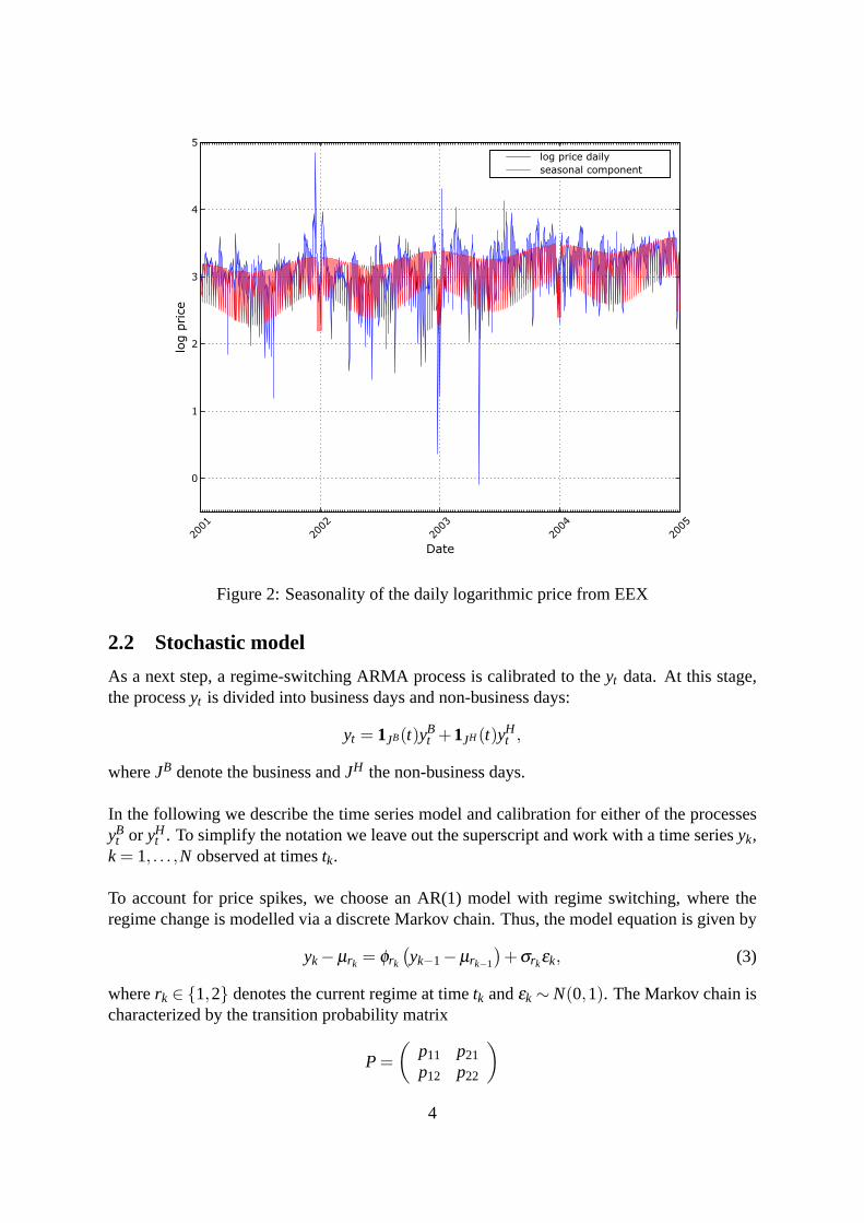
The regression model is solved using a least squares algorithm. An example of the seasonalcomponent is given in figure 2.

3

2001

2002

2003

2004

2005

Date

0

1

2

3

4

5

log p

rice

log price daily

seasonal component

Figure 2: Seasonality of the daily logarithmic price from EEX

2.2 Stochastic model

As a next step, a regime-switching ARMA process is calibrated to theyt data. At this stage,the processyt is divided into business days and non-business days:

yt = 1JB(t)yBt +1JH (t)yH

t ,

whereJB denote the business andJH the non-business days.

In the following we describe the time series model and calibration for either of the processesyB

t or yHt . To simplify the notation we leave out the superscript and work with a time seriesyk,

k = 1, . . . ,N observed at timestk.

To account for price spikes, we choose an AR(1) model with regime switching, where theregime change is modelled via a discrete Markov chain. Thus, the model equation is given by

yk−µrk = φrk

(yk−1−µrk−1

)+σrkεk, (3)

whererk ∈ {1,2} denotes the current regime at timetk andεk ∼N(0,1). The Markov chain ischaracterized by the transition probability matrix

P =(

p11 p21

p12 p22

)4

with pi j = P(r i = j | rk−1 = i).

Since the regime state is not observable we use the Hamilton filter described in [5]. Sincethe Hamilton filter requires the transition probabilities to depend only on the current state,we have to transform the two-state model above into a four-state model (see [5], p. 691) withstates ˜rk ∈ {1,2,3,4}, such that

rk = 1 if rk = 1 andrk−1 = 1

rk = 2 if rk = 2 andrk−1 = 1

rk = 3 if rk = 1 andrk−1 = 2

rk = 4 if rk = 2 andrk−1 = 2.

The transition probability matrix becomes

P =

p11 0 p11 0p12 0 p12 00 p21 0 p21

0 p22 0 p22

In this way, the model is of the general form

yk = µrk + φrkyk−1 + σrkεk. (4)

The Hamilton filter produces estimatesξ ik|k for the probabilityP(rk = i | yk,yk−1, . . .) that the

observation was generated by regimei based on observations up to timek. As a byproduct ofthe Hamilton filter, the log maximum likelihood function is calculated as

L =Nk

∑k=1

log

(4

∑i=1

ξik|kη

ik

)(5)

Example calibration results for EEX spot price data from Jan 01 to May 05 are the following:

µ φ σ

regime 1 −0.004 0.74 0.11regime 2 −0.02 0.68 0.30

P =(

0.94 0.280.06 0.72

)

Since we have only estimated probabilities about the regime during the calibration period, wecan only calculate estimates about the residuals:

εk = E[εk] =4

∑i=1

P(rk = i | yk,yk−1, . . .)(

yk− µi − φiyk−1

σi

)A sample autocorrelation function ofνk is shown in figure 3. Figure 4 shows a QQ plot forthe innovations both for the regime-switching process with two regimes and a non regime-switching AR(1) process. Using a simple AR(1) process instead of the regime-switchingprocess, the innovations are clearly non-Gaussian. The innovationsεk of the regime-switchingprocess provide a much better fit to a Gaussian distribution.

5

0 2 4 6 8 10 12 14 16 18 20−0.2

0

0.2

0.4

0.6

0.8

Lag

Sam

ple

Aut

ocor

rela

tion

Sample Autocorrelation Function (ACF)

Figure 3: Autocorrelation of EEX daily price residuals (Jan 01 – Apr 05)

−4 −3 −2 −1 0 1 2 3 4−6

−4

−2

0

2

4

6

8

Standard Normal Quantiles

Qua

ntile

s of

Inpu

t Sam

ple

QQ Plot of Sample Data versus Standard Normal

no regime−switchingregime−switching

Figure 4: QQ Plot of innovations for daily price process (EEX Data Jan 01 – Apr 05)

3 The Hourly Profile Process

From equation 1 the profile process is defined as the logarithmic spot process normalized tomean zero:

ht = st −st

The steps for modelling the profile dynamics are the following:

1. de-seasonalize the profile for each hour

2. use PCA to decompose the vector process into factor loads

3. model each factor load as an ARMA process

6

3.1 Seasonality and PCA decomposition

Daily spot price profiles have a pronounced yearly and weekly seasonality (see figure 5) due todifferent temperature and light conditions. To de-seasonalize the profiles a similar techniqueas described in section 2.1 is used for each single hour. In this way the profiles can be writtenas

ht = ht +∆ht ,

whereht is the deterministic seasonal component and∆ht is the stochastic residual from theregression.

0 5 10 15 20

Hour

0.5

1

1.5

2

Value

summerwinter

Figure 5: Mean summer and winter hourly profiles

The residuals∆ht form a vector process with a covariance structure reflecting the differentvolatilities of each single hour and the correlations between the hourly profile values. Asbefore, the process∆ht is divided into business days and non-business days:

∆ht = 1JB(t)∆hBt +1JH (t)∆hH

t .

The two processes∆hBt and∆hH

t are treated separately. For notational convenience we re-gard only one of these processes and denote it by∆hk, k = 1, . . . ,N. By means of a PCAthe vector process∆hk is now decomposed into independent factor loads. Letp1, . . . ,p24 bethe principal components of∆hk (after column-wise normalization to standard deviation 1),i. e. the eigenvectors of the matrix(∆h)T∆h/N, where∆h is aN×24-matrix. It is assumedthat the corresponding eigenvalues are in descending orderλ1 > .. . > λ24. The 24×24-matrix(p1, . . . ,p24) containing the principal components as columns is denoted byP. TheN×24-matrix of factor loads is then given byZ = (∆h)P. An example of the principal componentsis shown in figure 6.

7

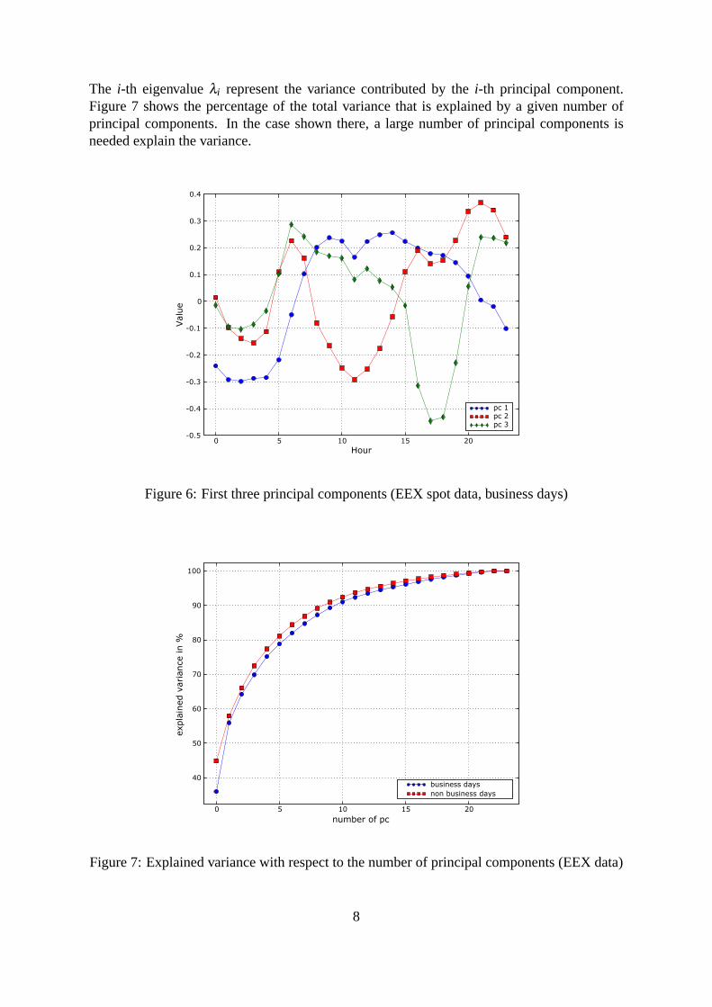
The i-th eigenvalueλi represent the variance contributed by thei-th principal component.Figure 7 shows the percentage of the total variance that is explained by a given number ofprincipal components. In the case shown there, a large number of principal components isneeded explain the variance.

0 5 10 15 20

Hour

-0.5

-0.4

-0.3

-0.2

-0.1

0

0.1

0.2

0.3

0.4

Valu

e

pc 1pc 2pc 3

Figure 6: First three principal components (EEX spot data, business days)

0 5 10 15 20

number of pc

40

50

60

70

80

90

100

expla

ined v

ariance in %

business days

non business days

Figure 7: Explained variance with respect to the number of principal components (EEX data)

8

3.2 Stochastic model

Let zik = Zk,i , i = i, . . . ,24,k = 1, . . . ,N be the time series of thei-th factor load, which is the

i-th column of the matrixZ. The serieszik are modelled as independent ARMA process. From

the simulated factorloadsZ the process∆ht can be calculated as∆ht = ZPT .

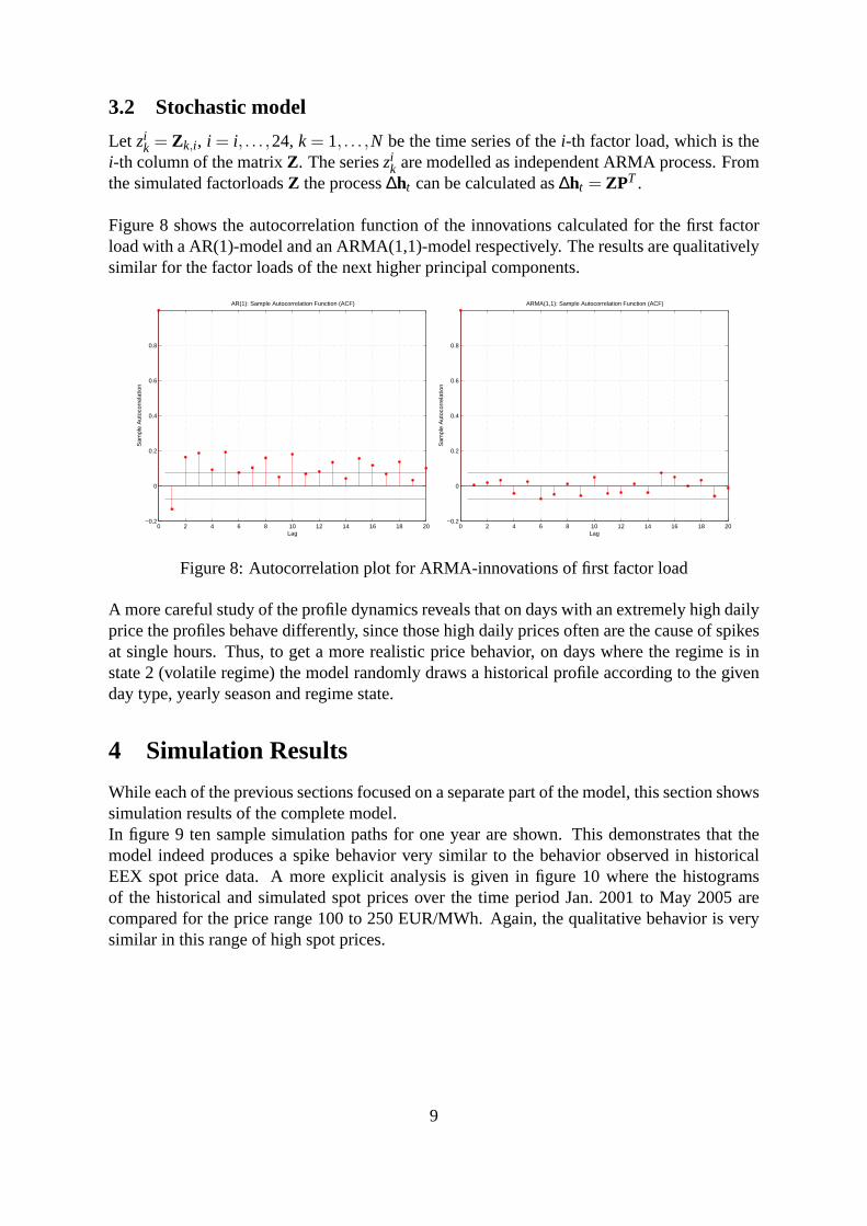
Figure 8 shows the autocorrelation function of the innovations calculated for the first factorload with a AR(1)-model and an ARMA(1,1)-model respectively. The results are qualitativelysimilar for the factor loads of the next higher principal components.

0 2 4 6 8 10 12 14 16 18 20−0.2

0

0.2

0.4

0.6

0.8

Lag

Sam

ple

Aut

ocor

rela

tion

AR(1): Sample Autocorrelation Function (ACF)

0 2 4 6 8 10 12 14 16 18 20−0.2

0

0.2

0.4

0.6

0.8

Lag

Sam

ple

Aut

ocor

rela

tion

ARMA(1,1): Sample Autocorrelation Function (ACF)

Figure 8: Autocorrelation plot for ARMA-innovations of first factor load

A more careful study of the profile dynamics reveals that on days with an extremely high dailyprice the profiles behave differently, since those high daily prices often are the cause of spikesat single hours. Thus, to get a more realistic price behavior, on days where the regime is instate 2 (volatile regime) the model randomly draws a historical profile according to the givenday type, yearly season and regime state.

4 Simulation Results

While each of the previous sections focused on a separate part of the model, this section showssimulation results of the complete model.In figure 9 ten sample simulation paths for one year are shown. This demonstrates that themodel indeed produces a spike behavior very similar to the behavior observed in historicalEEX spot price data. A more explicit analysis is given in figure 10 where the histogramsof the historical and simulated spot prices over the time period Jan. 2001 to May 2005 arecompared for the price range 100 to 250 EUR/MWh. Again, the qualitative behavior is verysimilar in this range of high spot prices.

9

Jan 06

Feb 06

Mar

06

Apr

06

May

06

Jun 06

Jul 0

6

Aug

06

Sep

06

Oct 06

Nov

06

Dec

06

Jan 07

Date

0

200

400

600

800

1000

1200

1400

1600

Hourly P

rice E

UR/M

Wh

path 1

path 2

path 3

path 4

path 5

path 6

path 7

path 8

path 9

path 10

Figure 9: Ten sample hourly EEX spot simulation paths for year 2006

100 150 200 2500

0.5

1

1.5

2

2.5

3

3.5

x 10−3

spot price in EUR/MWh

freq

uenc

y

historical datasimulated data

Figure 10: Histogram of historical and simulated spot prices in the range 100− 250EUR/MWh

10

References

[1] M. Bierbrauer, S. Trück, and R. Weron Modelling electricity prices with regime switch-ing models Lecture Notes in Computer Sciences, 07/2004

[2] M. Burger, B. Klar, A. Müller, G. Schindlmayr A spot market model for pricing deriva-tives in electricity markets. Quantitative Finance, Vol. 4, pp. 109-122, 2004

[3] C. De Jong, R. Huisman, Option formulas for mean-reverting power prices with spikes,Working Paper, Erasmus University Rotterdam, 2002.

[4] S. Deng, Stochastic Models of Energy Commodity Prices and Their Applications: Mean-reversion with Jumps and Spikes, Working paper, Georgia Institute of Technology, 2000.

[5] J. D. Hamilton. Time Series Analysis. Princeton University Press, 1994

[6] A. Roncoroni, H. Geman, A class of marked point processes for modelling electricityprices, Working Paper, ESSEC, 2003.

[7] P. Skantze, A. Gubina, M. Ilic, Bid-based stochastic model for electricity prices: Theimpact of fundamental drivers on market dynamics Report, MIT Energy Laboratory(2000).

11