A Roadmap to Estimation Using Balanced Productivity ... Proceedings/ISMA4-2009... · A Roadmap to...

Jim Mayes, CFPS 9000 Central Park West

Suite 800Atlanta, GA 30328

Phone: 678-443-1042email: [email protected]

A Roadmap to Estimation Using Balanced Productivity

Metrics: “$Right-Pricing”

May 15, 2009 Version 4.0

2

$Right-Pricing Software Projects

Underlying Themes for 2009 are “Change” and “The Economy”:

• In this tough economy, we need to analyze cost drivers related to software projects

• Can’t keep playing guessing games when estimating projects…like on “$The Price is Right”.

• Businesses need to find the “right price” for software projects with regard to business value.

• Estimates should provide alternative solutions, or tradeoffs, for making business decisions, not just one answer.

• Parametric modeling provides practical solutions for estimating and “$Right-Pricing” software projects.

© 2009 CBS Interactive

3

Index

• Balancing Time, Cost, and Quality:• A Software Project Post-Mortem – “$Wrong-Pricing”

• Balanced Productivity Metrics – “$Right-Pricing”

• Estimation and Planning using Balanced Productivity Metrics:• A Practical Implementation of Parametric Estimation

• Simple Parametric Estimation Model• Time, Cost and Quality Tradeoff Calculator

• Conclusion• Backup Slides

4

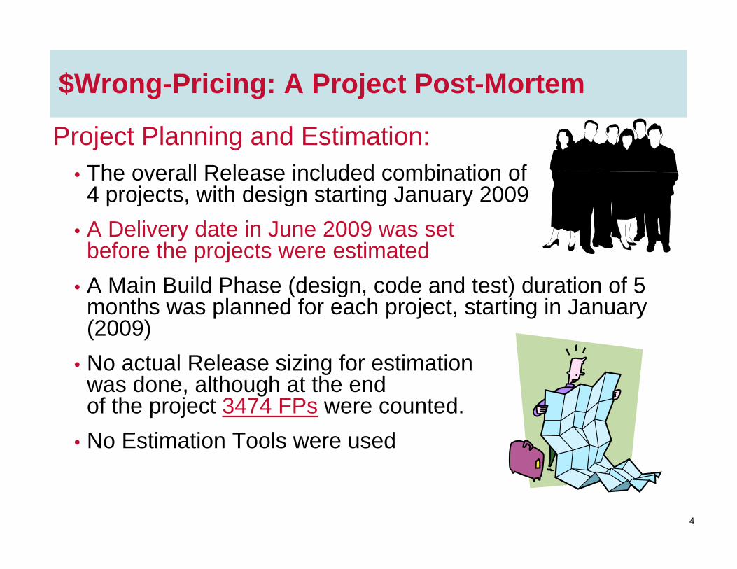
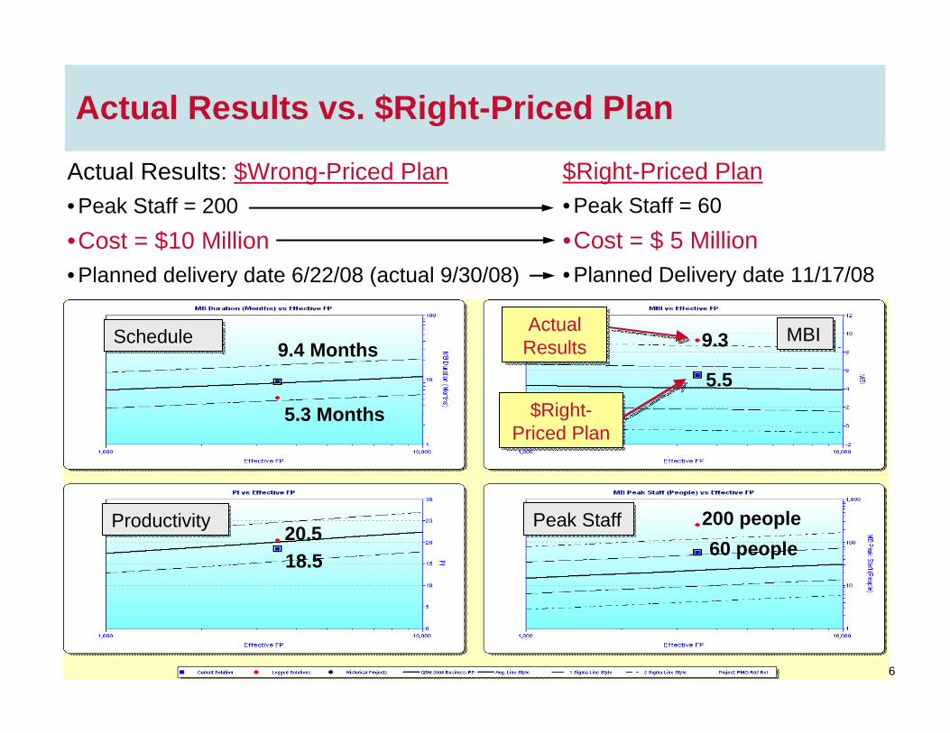
$Wrong-Pricing: A Project Post-Mortem

Project Planning and Estimation:• The overall Release included combination of

4 projects, with design starting January 2009• A Delivery date in June 2009 was set

before the projects were estimated• A Main Build Phase (design, code and test) duration of 5

months was planned for each project, starting in January (2009)

• No actual Release sizing for estimation was done, although at the end of the project 3474 FPs were counted.

• No Estimation Tools were used

5

A Project Post-Mortem

Actual Results:• Aggregate project staffing required over

200 people (Client IT and 4 Different Vendors) • People worked at times up to 36 hours without

sleep trying to complete the project on schedule• The project did not finish in June 2009 as planned and

testing is still going on through September due to a high volume of defects

• The client was extremely unhappy, heroic effort went unrewarded, and the team morale suffered.

“Are we there yet?”

6

Post-Mortem Benchmark Assessment

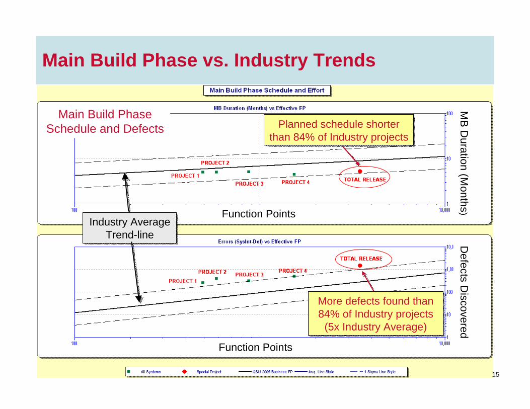
The QSM SLIM-Suite and Industry Data were used for the assessment:•Schedule compression was higher than 98% of Industry Projects (original planned completion date -6/22/09)•Main Build Phase schedule (Design, Coding, and Testing) was shorter than 84% of Industry projects•Main Build Phase effort and peak staff (200 people) was higher than 98% of Industry projects•The number of defects found from the Start of System through UAT was higher than 84% of Industry Projects (5x Industry Average)

7

Schedule Compression• Schedule compression causes exponentially increased effort, cost & defects• Schedule compression causes incomplete and overlapping project phases,

particularly the testing phases• Schedule compression is defined as the ratio of schedule to effort, called the

Manpower Buildup Index (MBI) in QSM terminology• Simplified illustration of the MBI equation: A Manpower Buildup Value is

calculated and converted into a Manpower Buildup Index (MBI) with a range of -3 (low) to 10 (High).

“Please be aware that this software equation was derived empirically: It’s not anybody’s theory about how effort ought to vary as schedule is compresses; it’s the observed pattern of how it has varied.” – Tom Demarco

=TOTAL EFFORT

TIMEMBI

8

Peak Staff vs. Industry Trend-lines

QSM Industry Average Trend-line

QSM Industry Average Trend-line

Total Main Build Phase (Design, Code, Test) Peak Staff is higher than

98% of all Industry projects

Total Main Build Phase (Design, Code, Test) Peak Staff is higher than

98% of all Industry projects

Function Points

MB

Peak Staff (People)

200 People

68% 96% 99.8%

% of Projects within each Std. Dev. Range (+-1, +-2, & +-3 SD)

% of Projects within each Std. Dev. Range (+-1, +-2, & +-3 SD)

9

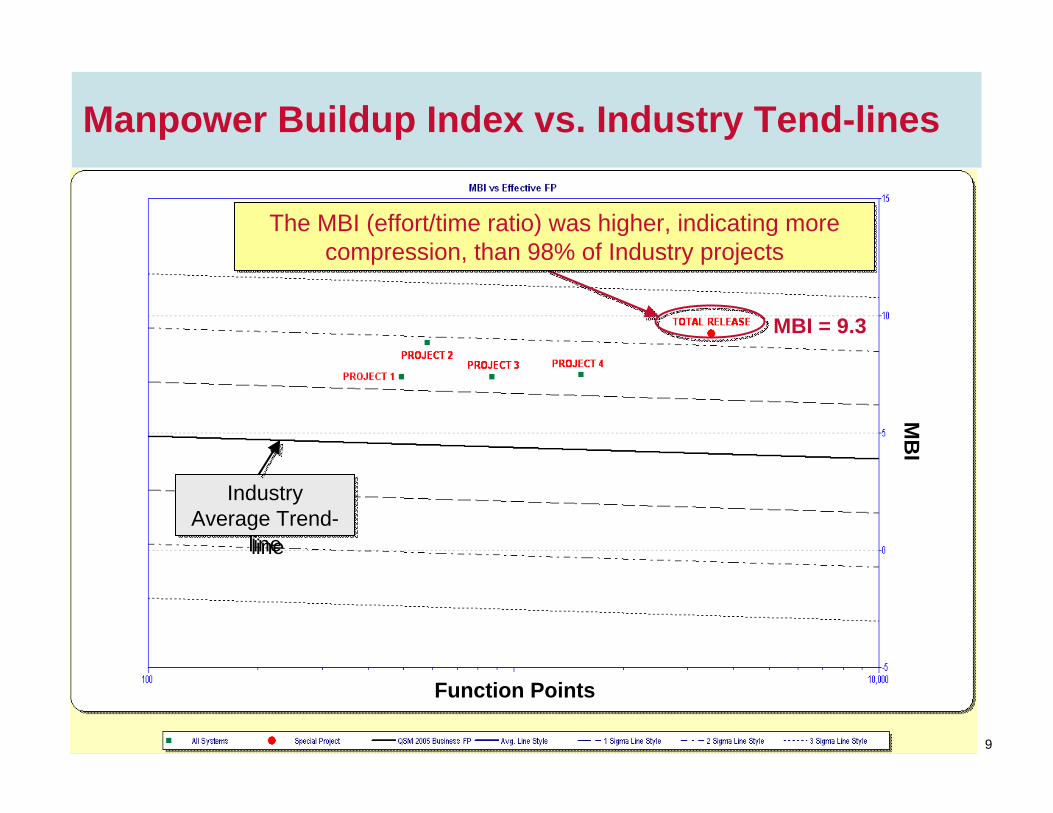
Manpower Buildup Index vs. Industry Tend-lines

Industry Average Trend-

line

Industry Average Trend-

line

The MBI (effort/time ratio) was higher, indicating more compression, than 98% of Industry projects

The MBI (effort/time ratio) was higher, indicating more compression, than 98% of Industry projects

MBI = 9.3

MB

I

Function Points

10

0

10

20

30

40

50

60

70

1 2 3 4 5 6 7 8 9 10 11 12 13

Staffing

Elapsed Time

• 6 People• $416,000• MTTD = 4.8 Days

• 24 People• $1,300,000• MTTD = 1.2 Days

• 66 People• $3,000,000• MTTD = .4 Days

MBI =1MBI = 2

MBI = 3

MBI = 4

MBI = 5

MBI = 6

How Staffing Levels Impact Time, Cost, & Quality

Example: Size = 75,000 SLOCPI = 16

MTTD = Mean Time To Defect (number of days between the discovery of defects during the 1st 30 days of Production)

= 12 Mo.

= 10 Mo.

= 8 Mo.

11

There is a exponential growth in Communication Complexity as schedules are compressed and more people are added.

CommunicationComplexity

Number of People

ErroneousCommunication =

Defects

Remember Fred BrooksThe Mythical Man month


12

Project Staff of 4 people = 4(3 paths)/2 = 6 pairs or 12 communication paths (counting both directions)

1

2

3

4

Mythical Man-Month Formula: n(n-1)/2 =

Communications Pairs


13

Project Staff of 8 people = 8(7 paths)/2 = 28 pairs or 56 communication paths (counting both directions)

1

2

3

4

56

78

Increased complexity of inter-

communicationwhen staff is increased.


14

Example Project:Size = 75,000 SLOC (Source Lines of Code)PI (Productivity Index) = 16

MBI (ManpowerBuildup Index)

PeakStaff

Schedule(Months)

Cost($)

123456

69

14243366

13.612.311.310.2

9.58.3

416,000623,000875,000

1,300,0001,700,0003,000,000

Mean Time To Defect (Days)*

4.83.22.11.20.90.4

Group Communication Paths = n(n-1)/2• 33 People: 33(33-1)/2 = 528 Communication Pairs• 66 People: 66(66-1)/2 = 2,145 Communication Pairs• Project: 200(200-1)/2 = 19,900 Communication Pairs


*Note: MTTD = Number of days between the discovery of a new defect.

15

Main Build Phase vs. Industry Trends

Industry Average Trend-line

Industry Average Trend-line

Planned schedule shorter than 84% of Industry projects

Planned schedule shorter than 84% of Industry projects

Main Build Phase Schedule and Defects

Function Points

Function Points

MB

Duration (M

onths)D

efects Discovered

More defects found than 84% of Industry projects

(5x Industry Average)

More defects found than 84% of Industry projects

(5x Industry Average)

16

Actual Results vs. $Right-Priced Plan

Actual ResultsActual Results

$Right-Priced Plan

$Right-Priced Plan

ScheduleSchedule

ProductivityProductivity

MBIMBI

Peak StaffPeak Staff

$Right-Priced Plan• Peak Staff = 60•Cost = $ 5 Million• Planned Delivery date 11/17/08

9.3

5.5

Actual Results: $Wrong-Priced Plan• Peak Staff = 200•Cost = $10 Million• Planned delivery date 6/22/08 (actual 9/30/08)

200 people60 people

20.518.5

9.4 Months

5.3 Months

17

Index



• Estimation and Planning Using Balanced Productivity Metrics:• A Practical Implementation of Parametric Estimation



18

Principles of Balanced Productivity Metrics

• “A balanced set of measurements helps prevent dysfunctional behavior by estimating and monitoring performance in several complementary aspects of work that lead to project success.”

• Estimation theory is a branch of statistics that deals with estimating the values of parameters based on measured/empirical data. • An estimator attempts to approximate the unknown parameters

using the measurements.

• Provides historical estimates as opposed to hysterical estimates

• The objective of any software estimate is to optimize time, cost and quality relative to the expected business value or ROI to be received from the software product.

• In the Project Post-Mortem: Was time-to-market and worth the extra $5 Million it cost to compress the schedule?

19

Balancing Time, Cost, and Quality

Time

Cost

QualityCustomer Satisfaction& Business Objectives

Business Value(shorter schedule)

IncreasedEffort/Cost

IncreasedDefects

20

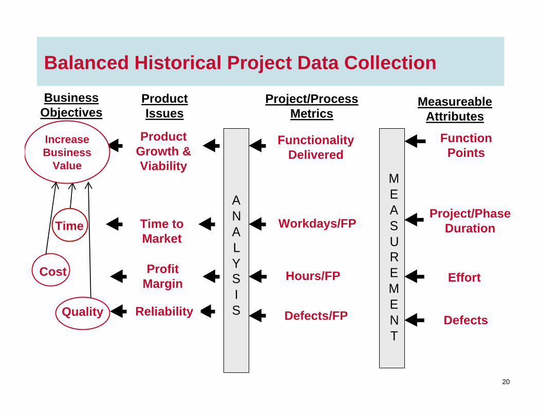
Balanced Historical Project Data Collection

BusinessObjectives

Project Issues Process IssuesMeasurable Product& Process Attributes

Number of defectsintroduced &effectiveness ofdefect detectionactivities

Number ofrequirements,product size,productcomplexity, ratesof change, & %non-conforming

Product conformance

ANALYSIS

Product growth& stability

Budgets &expenditurerates

Productperformance,productcorrectness,product reliability

Production rate &responsiveness

Efficiency,productivity, &rework

Predictability,problem recognition,& root cause analysis

ENHANCEBUSINESSVALUE

COST

QUALITY

MEASUREMENT

Product size,complexity, effort,# changes, &requirementsstability

Elapsed time &normalizedproductcharacteristics

Scheduleprogress

TIME

Functionality Delivered

Effort

Defects

Hours/FP

Workdays/FP

Defects/FP

Function Points

Product Issues

Project/Process Metrics

Measureable Attributes

Product Growth & Viability

Profit Margin

Time to Market

Reliability

Business Objectives

Increase Business

Value

Time

Cost

Quality

Project/Phase Duration

21

$Right-Pricing: Analysis of Historical Project Data

Optimal Project Size Range for

the Organization

Optimal Project Size Range for

the Organization

30,000 to

140,000 SLOC

Standard Deviation Trend-lines (+- 1, 2, & 3)

Standard Deviation Trend-lines (+- 1, 2, & 3)

Historical Projects Data

Points

Historical Projects Data

Points

Productivity (PI)

SLOC (000)

Average Trend-lineAverage

Trend-line

Bell-shaped Productivity

Curve

Bell-shaped Productivity

Curve

22

RNS 1999/2000 Releases vs. Main Build Trends (BellSouth PI)

PI vs ESLOC BellSouth 1997-1999 Comparison

Effective SLOC (thousands)1 10 100 1000 10000

PI

-10

0

10

20

30

40

50

RNS July 2000.5

RT/VNS IntegrationRNS June 2000.4

RNS Credit ChallengedRNS BellSouth Voice Mail

RNS/VNS Project One

All Systems Special Project Avg. Line Style 1 Sigma Line Style 2 Sigma Line Style3 Sigma Line Style

30,000 to150,000ESLOC

Optimal SizeRange forBellSouth Projects

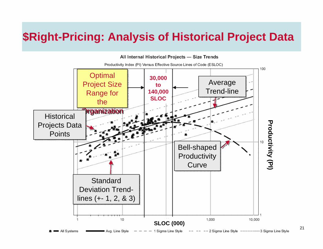
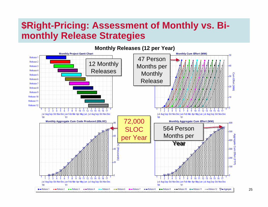
$Right-Pricing: Assessment of Monthly vs. Bi-monthly Release Strategies

Smaller Releases (6K) = Lower ProductivitySmaller Releases (6K) = Lower Productivity

Optimal Project Size

Range for the Organization

Optimal Project Size

Range for the Organization

30,000 to

140,000 SLOC

Productivity

Size (SLOC)

Larger Releases (44K) = Higher ProductivityLarger Releases (44K) = Higher Productivity

23

RNS 1999/2000 Releases vs. Main Build Trends (BellSouth MBI)

MBI vs Effective SLOC

Effective SLOC (thousands)1 10 100 1000 10000

MBI

-5

0

5

10

15

20

RNS June 2000.4

RNS July 2000.5

RNS/VNS Project One

RNS Credit ChallengedRNS BellSouth Voice Mail

RT/VNS Integration

All Systems Special Project Avg. Line Style 1 Sigma Line Style 2 Sigma Line Style3 Sigma Line Style

30,000 to

140,000 SLOC

Optimal Size Range

Optimal Size Range

MBI 5 to 6


Smaller Projects (6K) = 6.7 Avg. MBI

Smaller Projects (6K) = 6.7 Avg. MBI Larger Projects (44K)

= 5.4 Avg. MBILarger Projects (44K)

= 5.4 Avg. MBI

Optimal MBI Range related to Optimal Size

Optimal MBI Range related to Optimal Size

Manpow

er Buildup Index (M

BI)

Size (SLOC)

24

• Monthly releases - Assumptions: • Monthly releases are based on an average of historical

small projects (5.2 months duration, 6,000 ESLOC, 6.7 MBI, 47 Person Months, .63 MTTD, including the Planning, Analysis, and Main Build Phases).

• This illustrates 12 monthly releases during the year.

• Bi-monthly releases – Assumptions:• Bi-monthly releases were based upon historical large

projects (7 months duration, 44,000 ESLOC, 5.4 MBI, 94 Person Months, 1.1 MTTD, including the Planning, Analysis, and Main Build Phases).

• This illustrates 6 Bi-monthly releases during the year.


25

RNS Monthly Releases vs. Total Effort and ESLOC Produced

Monthly Project Gantt Chart

1 2 3 4 5 6 7 8 9 10 11 12 13 14 15 16 17Jul'00

Aug Sep Oct Nov Dec Jan'01

Feb Mar Apr May Jun Jul Aug Sep Oct Nov Dec

Release 1

Release 2

Release 3

Release 4

Release 5

Release 6

Release 7

Release 8

Release 9

Release 10

Release 11

Release 12

Monthly Cum Effort (MM)

1 2 3 4 5 6 7 8 9 10 11 12 13 14 15 16 17Jul'00



Cum

Effort (MM

)

0

10

20

30

40

50

Monthly Aggregate Cum Code Produced (ESLOC)

1 2 3 4 5 6 7 8 9 10 11 12 13 14 15 16 17Jul'00



ESLOC

(thousands)

0

20

40

60

80 Monthly Aggregate Cum Effort (MM)

1 2 3 4 5 6 7 8 9 10 11 12 13 14 15 16 17Jul'00



Aggregate Cum

Effort (FTP)

0

100

200

300

400

500

600

Release 1 Release 2 Release 3 Release 4 Release 5 Release 6 Release 7 Release 8 Release 9 Release 10 Release 11 Release 12 Aggregate

47 Person Months per

Monthly Release


Monthly Release


12 Monthly Releases

12 Monthly Releases


Year


Year

Monthly Releases (12 per Year)

72,000 SLOC

per Year

72,000 SLOC

per Year

26

RNS Bi-Monthly Releases vs. Total Effort and ESLOC ProducedMonthly Project Gantt Chart

1 2 3 4 5 6 7 8 9 10 11 12 13 14 15 16 17Jul'00



Release L1

Release L2

Release L3

Release L4

Release L5

Release L6

Monthly Cum Effort (MM)

1 2 3 4 5 6 7 8 9 10 11 12 13 14 15 16 17Jul'00



Cum

Effort (MM

)

0

20

40

60

80

100

120

Monthly Aggregate Cum Code Produced (ESLOC)

1 2 3 4 5 6 7 8 9 10 11 12 13 14 15 16 17Jul'00



ESLOC

(thousands)

0

50

100

150

200

250

300

350 Monthly Aggregate Cum Effort (MM)

1 2 3 4 5 6 7 8 9 10 11 12 13 14 15 16 17Jul'00



Aggregate Cum

Effort (FTP)

0

100

200

300

400

500

600

700

Release L1 Release L2 Release L3 Release L4 Release L5 Release L6 Aggregate


Year


Year


Monthly Release


Monthly Release

6 Bi-monthly

Releases

6 Bi-monthly

Releases


Bi-Monthly Releases (6 per Year)

264,000 SLOC

per Year

264,000 SLOC

per Year

27

• Conclusion: 6 Bi-monthly releases per year produces 267% more code than 12 Monthly releases, for the same effort and cost, with 31% better quality:• Twelve Monthly Releases, completing 1/14 - 12/14, produce

72,000 SLOC and require 564 Person Month’s.

• Six Bi-Monthly Releases, completing 2/14 - 12/14, produce 264,000 SLOC and require 564 Person Month’s.

• Individual Bi-monthly releases are 26% longer (7 months each) than Monthly releases (5.2 months each).

• MTTD (at deployment) for each Bi-monthly releases is one defect every 1.1 days, versus one defect every .63 days (1.6 defects per day) for each Monthly release.

• Total Post Delivery phase effort and cost for defect correction would be 58% less with six Bi-monthly releases.


28

Index



• Estimation and Planning using Balanced Productivity Metrics:• A Practical Implementation of Parametric Estimation



29

Parametric Approach to Estimation

• Parametric modeling is used for estimating the duration, cost, reliability and risk tradeoffs on software development projects.

• Estimates/Plans are based on internal historical performance data, supplemented by Industry Data.

• The management alternatives for each project can be evaluated and sanity checked with internal history and industry data, even before any task level planning occurs.

• Parametric modeling is used for estimating the duration, cost, reliability and risk tradeoffs on software development projects.

• Estimates/Plans are based on internal historical performance data, supplemented by Industry Data.

• The management alternatives for each project can be evaluated and sanity checked with internal history and industry data, even before any task level planning occurs.

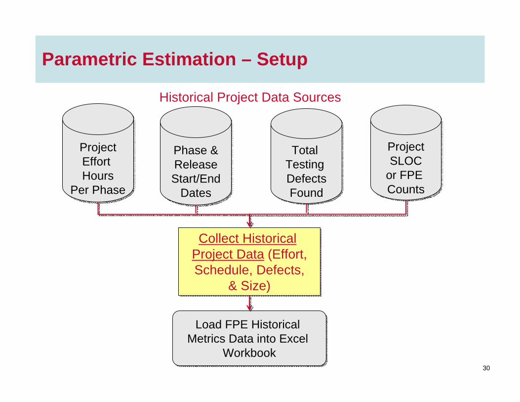
ProjectSLOC

or FPE Counts

ProjectSLOC

or FPE Counts

30

Parametric Estimation – Setup

Collect Historical Project Data (Effort,Schedule, Defects,

& Size)

Collect Historical Project Data (Effort,Schedule, Defects,

& Size)

ProjectEffort Hours

Per Phase

ProjectEffort Hours

Per Phase

Phase &ReleaseStart/End

Dates

Phase &ReleaseStart/End

Dates

Total Testing DefectsFound

Total Testing DefectsFound

Historical Project Data Sources

Load FPE Historical Metrics Data into Excel

Workbook

Load FPE Historical Metrics Data into Excel

Workbook

31

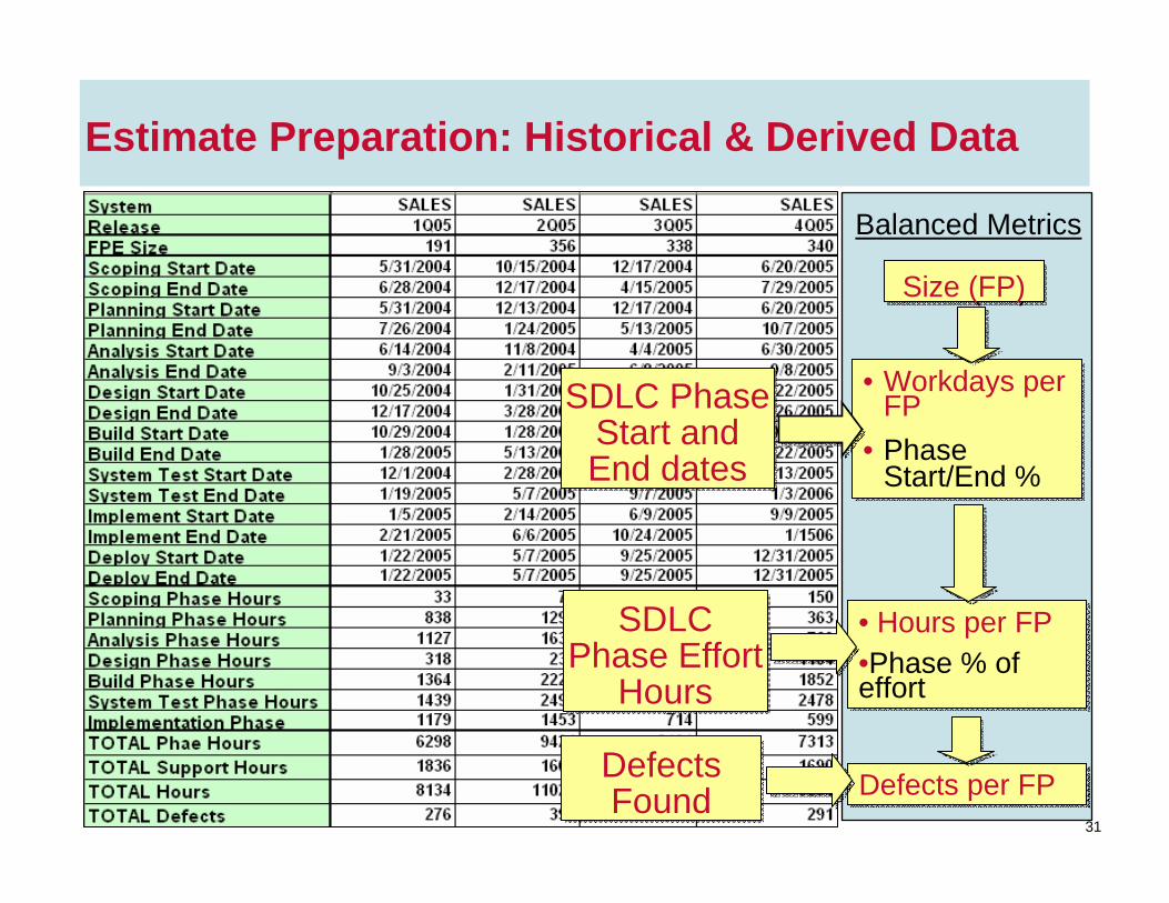
Estimate Preparation: Historical & Derived Data

• Workdays per FP

• Phase Start/End %

• Workdays per FP

• Phase Start/End %

• Hours per FP•Phase % of effort

• Hours per FP•Phase % of effort

Defects per FPDefects per FP

Size (FP)Size (FP)

SDLC Phase Start and End dates

SDLC Phase Start and End dates

SDLC Phase Effort

Hours

SDLC Phase Effort

Hours

Defects Found

Defects Found

Balanced Metrics

32

Simple Parametric Estimation Model

Enter Project Size(Function Points)

Enter Project Size(Function Points)

Select Data and Enter Factors from Similar Historical

Projects

Select Data and Enter Factors from Similar Historical

Projects

1 Enter Size UncertaintyLevel (Low = +10%,

Medium = +30%,High = +50%)

Enter Size UncertaintyLevel (Low = +10%,

Medium = +30%,High = +50%)

2 3

1 2 3

Run Phase Effort and Schedule Calculator

Run Phase Effort and Schedule Calculator

33

• Release Start Date 2/1/09• Total Hours = 11,224• Total Workdays = 197

100% = 197 Workdays

11/3/09

86.6% = 171 Workdays

9/25/09

0% = 0 Workdays

2/1/09

0.9% * 11,224 = 99 Scoping Effort Hours

Schedule Timeline

Enter PhaseEffort and Schedule

Tuning Factors

Enter PhaseEffort and Schedule

Tuning Factors

4

Phase Effort and Schedule Calculator

34

Evaluate Business Objectives & Constraints

Cost Constraints:•What are the cost constraintsrelated to business objectives?

•What is the desired probabilityfor not exceeding this cost?

Time Constraints:•What is the business driverwith regard to a schedule?

•What is the desiredprobability for not exceedingthis deadline?

Quality Constraints•What is range of reliability thatwould be desired or minimallyacceptable for desired value?

•What is the desired probabilityfor not exceeding this level?

COST

TIME QUALITY

Amount_ $

%

Customer Satisfaction& Business Objectives

Amount______Months

%

Amount_ _____Defectsper day

%

1.5M

90

10

65

1

40

• Assess Business Objectives

• Develop Priorities• Align Constraints• Plan Proactively• Tradeoff Analysis

$Right-Pricing$Right-Pricing

35

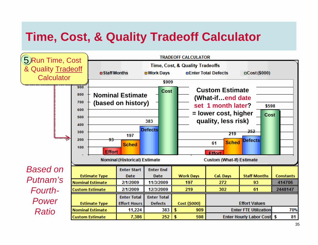
Run Time, Cost& Quality Tradeoff

Calculator

Run Time, Cost& Quality Tradeoff

Calculator

5

Time, Cost, & Quality Tradeoff Calculator

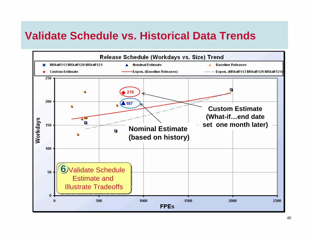
Nominal Estimate (based on history)

Custom Estimate (What-if…end date set 1 month later? = lower cost, higher

quality, less risk)

Based on Putnam’s Fourth-Power Ratio

Effort

Cost

Defects

Sched

Cost

DefectsSched

Effort

36

Index

• Part 1 – Balancing Time, Cost, and Quality:• A Software Project Post-Mortem – “$Wrong-Pricing”


• Part 2 – Estimation and Planning using Balanced Productivity Metrics:• A Practical Implementation of Parametric Estimation



37

Conclusion• Determine business drivers associated with projects relative to

time, cost, and quality:• One estimate doesn’t fit all situations; Projects should be “$Right-Priced”• Analyze the tradeoffs and provide alternative solutions for making

business decisions• Use a balanced set of data to tune estimates:

• Data provide a historical basis for estimates• One metric, such as hours per Function Point or KSLOC, does not

provide the desired outcome• Effort Productivity Measures such as hours per FP, only have meaning

when used within the relative context associated with schedule and quality results

• In tough economic times there is more attention to cost:• Be an champion of change in the way projects are planned• Use software metrics data and parametric modeling to improve

estimates, provide lower cost options, and achieve business objectives

38

For Questions or Additional Information

Contact:

Jim Mayes, CFPSCGI Senior Consultant

Email: [email protected]

Office Phone: 678-443-1042

39

Index

• Part 1 – Balancing Time, Cost, and Quality:• A Software Project Post-Mortem – “$Wrong-Pricing”


• Part 2 – Estimation and Planning using Balanced Productivity Metrics:• A Practical Implementation of Parametric Estimation



40

Validate Schedule Estimate and

Illustrate Tradeoffs

Validate Schedule Estimate and


6

Validate Schedule vs. Historical Data Trends


Custom Estimate (What-if…end date

set one month later)

41

Validate Effort vs. Historical Data Trends


Custom Estimate (What-if…end date set

one month later?)

Validate Effort Estimate and


Validate Effort Estimate and


6

42

Validate Defects vs. Historical Data Trends


Custom Estimate (What-if…end date set

one month later?)

Validate QualityEstimate and


Validate QualityEstimate and


6

43

Time, Cost, & Quality Tradeoff Calculator


Custom Estimate (What-if…end date

set 1 month earlier ? = higher cost, lower quality, higher risk)

Sched SchedEffort Effort

Defects

Defects

Cost

Cost

44

• The computational Putnam (SLIM) software equation:

• Effort = [Size * B1/3 / Productivity Parameter]3 * 1 / Time4

• For any particular system or project estimate, the terms in the bracket are constant (size and productivity)

• Therefore, the Fourth-Power Ratio for tradeoff analysis is :

• Effort = Constant / Time4

• This is Putnam’s Effort Time Tradeoff Law.• Empirically derived and verified

Tradeoff Calculator: Putnam’s Fourth-Power Ratio

45

Bring It On Home

• Size Completed Projects (at least 3 for each System or Team)• Collect other Historical Project Data

• Effort Hours per Phase• Phase start and End dates• Defects• Size (FPE or SLOC)

• Build Tools:• Excel workbook to use for counting FPEs• Historical project data workbook• Estimation Model workbook

• Train for Project Teams on the Estimation Process• $Right-Priced Freebies: All templates shown in presentation

and the Simple Parametric Estimation/Tradeoff Models (doesn’t include trend charts) - leave me your card or leave name and email address

46

References1. Putnam and Myers. (1992) Measures For Excellence: Reliable Software On Time,

Within Budget. Yourdon Press/Prentice Hall.2. Demarco, Tom. (1982) Controlling Software Projects. Yourdon Press.3. Boehm, Abts, and Sunita. (2000). Software Development Cost Estimation

Approaches – A Survey. 4. International Function Point Users Group (IFPUG). Function Point Counting

Practices Manual, Release 4.2, Princeton, NJ: IFPUG, 2004.5. Paulk, Weber, Garcia, Chrissis, Bush. (1993). Key Practices of the Capability

Maturity Model, Version 1.1. CMU/SEI-93-TR-25, ESC-TR-93-178.6. Florac, Park, and Carleton. (1997) Practical Software Measurement: Measuring for

Process Management and Improvement. CMU/SEI-97-HB-003.7. Baumert and McKinney. (1992) Software Measures and the Capability Maturity

Model. CMU/SEI-92-TR-25, Technical Report. 8. Mayes, Jim. (2001, August). A Road Map for Balanced Productivity Metrics: Are

We There Yet? IT Metrics Strategies. Cutter Consortium.9. Mayes, Jim. (2000, March). Achieving Business Objectives: Balancing Time, Cost,

and Quality. IT Metrics Strategies. Cutter Consortium.10. Mayes, Jim. (2001, August). Saving the World, One Project at a Time: Planning by

the Numbers. IT Metrics Strategies. Cutter Consortium.

Date post:	09-Apr-2018
Category:	Documents
Upload:	phunganh
View:	215 times
Download:	0 times

A Roadmap to Estimation Using Balanced Productivity ... Proceedings/ISMA4-2009... · A Roadmap to...

Documents