Element stability are different in different solvent and different matrix.- Drift
It can have a dramatic effect on all analyses performed using ICP-MS. Drift ariseswhen an instrument response changes with time. Drift appears to be directly dependent on thematrix of the solution introduced to the ICP-MS. Typically, samples with moderate to hightotal dissolved solids contents will deposit salts on the cone orifices. This plating actionresults in a drop in sensitivity over time. The drift could be: a) linear as a function of time;b) a non-linear function of time but is independent of mass; c) Instrument response is anon-linear function of time and mass (see discussion on calibration below).
- Matrix effectsThe role that matrix plays is complex and varied, and can lead to dramatically reduce
the accuracy. Complex geological matrices generally result in a suppression of the analyte,although enhancements have been observed.
- Interference:Apart from isobaric overlap, recombination of ions leads to the formation of
interferences. There are different types of interferences:- The argon plasma: Ar+, Ar2+- Polyatomic species: Contribution from the solvent and combination with theanalyte species: (H2O+, H3O+, OH+, ArH+ etc….). Incomplete dissociation ofthe sample matrix will lead to recombination in the plasma tail, usually in theform of oxide MO+ (or MO2+, MO3+). The oxide formation will depend on theoxide bond strength of the element (quite high for REE for example).- Air entrainment and gas impurity (N+, O2+, NO2+, etc…)- Material eroded from the cones (isotopes of Ni, Cu, Mo etc…)
- Standardisation (calibration):Three methods for quantitative analysis available for the ICP-MS:
- Standard additions: In the case of standard additions, the technique involvestaking the sample, dividing it into equal aliquots, and adding to each increasing amounts of areagent containing the element(s) under consideration. The increments usually consist ofequal volumes, and a minimum of four mixtures is required per sample. Therefore, a set ofstandard addition "spikes" must be prepared and calibrated in addition to the preparation ofthe sample. Thus, for each sample analysed by standard additions at least four solutions mustultimately be measured. Standard additions can routinely yield data that is better than 2%
- Isotope dilution: Isotope dilution, while being a potentially extremely accuratetechnique, is also labour intensive and more costly than standard additions. Isotope dilutionmass spectrometry is based on the addition of a known amount of enriched isotope (called the"spike") to a sample. After equilibration of the spike isotope with the natural element in thesample, the ICP-MS is used to measure the altered isotope ratio. The difference between theisotopic ratio in the mixture and the natural isotope ratio can be used to accurately calculatethe concentration of the element in the sample. While the addition of spike is not particularlytime consuming, the initial time spent in preparing the spike solutions is. Additionally, theinitial cost of purchasing the spike solution can be high. A further disadvantage of isotopedilution is that the concentration in the unknown is generally a non-linear function of theisotope ratio of the standard-spike mixture. This non-linearity leads to error magnification,which becomes a serious problem when the isotope ratio in the sample-spike mixtureapproaches that of either the natural value or the spike value. Avoiding error magnificationrequires some knowledge of the concentration before spiking. IDMS produces data better than1%.
- External standardisation: External standardisation minimises effort but oftensacrifices precision. In the external standard calibration method, the blank-subtracted signalintensities for the element of interest in a group of standards are plotted against the knownconcentration of the element in those standards. A calibration curve is fitted to the data points.This technique is not as labour intensive as standard addition or isotope dilution, however it isnot as accurate. Using a straightforward classical approach, under optimal conditions ofinstrument tuning and maintenance, the ICP-MS produces results with a maximum precisionfor analysis of geological materials (i.e., complex matrices) in the range of 5 to 10 %.
The main problems associated with external calibrations are:- Dynamic range: Typically in the commercially available ICP-MS instruments,
the linear dynamic range, the range over which the response of the instrument is linear withrespect to analyte concentration, is greater than six orders of magnitude. As such, the curvefitted to the standard data should be linear. The slope of the line defined by the standards isproportional to the concentration in the standards. The unknown sample is run and its signalintensity is plotted against the curve to determine the concentration.
- Matrix effects: The role that matrix plays is complex and varied, and can lead todramatically diminished accuracy. Complex geological matrices generally result in asuppression of the analyte, although enhancements have been observed. One commonsuggestion is to match the matrices of the standards and unknowns. Using a suite of UnitedStates Geological Survey (USGS) standards encompassing the entire range of igneous rockcompositions from basalt to granite (e.g., BIR-1, DNC-1, W-2, BHVO-1, AGV-1, GSP-1, andG-2) results in non-linear calibration curves for the rare earth elements (REE). The maximumrange in concentrations in rare earths in this suite is less than 4 orders of magnitude, and thusis well within the linear dynamic range of the instrument. The non-linear portion of thecalibration curves involves AGV-1, GSP-1 and G-2, the 3 non-basaltic members of this suite.However basaltic rocks should be analysed against basaltic standards and granites againstgranitic standards.
- Drift: It can have a dramatic effect on all analyses performed using ICP-MS.Drift arises when an instrument response changes with time. The drift could be:
Figure 3.1: linear as a function of time; a non-linear function of time but is independent ofmass; a non-linear function of time and mass (from Cheatham et al 1993).
Instrument response is a non-linear function of time and mass.In reality, the analysis of geological samples with complex matrices is indeed a
complex function of time and mass, and that neither simple recalibration nor internalstandardisation adequately corrects for it. So long as matrices of samples and standards arewell matched, the drift is the single most important factor limiting analytical precision in ICP-MS analysis. Ideally, the matrix would have to be removed to avoid matrix effect, but thechemical processing required for matrix removal is generally labour intensive. Matrixremoval also introduces two other potential sources of analytical error: blank and yield. Thedevelopment of a method of drift correction is preferable to remove the matrix effect.
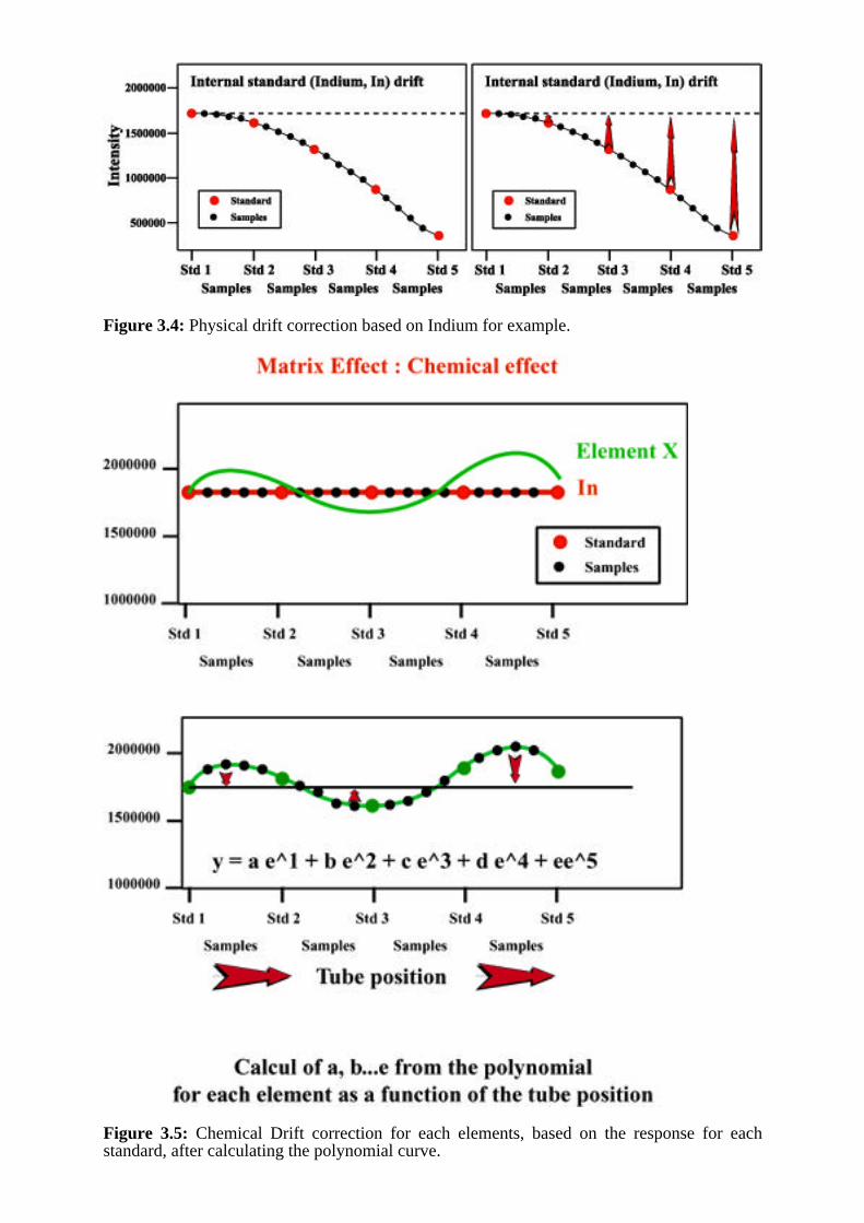
The technique is based on the analysis if a 'drift correction' standard after every 4 or 5samples. The sample and standards are mixed with an internal standard (e.g. 10ppb ofIndium). A first correction is applied for physical drift, while recalculating each samples driftbased on the signal given by the first standard (Figure 3.4). After the first drift correction forIndium, a polynomial curve is fit to each isotope analysed, and a correction is applied, basedon this curve to the measured intensity of the respective isotope in both sample and standardsolutions. Using this technique, the ICP-MS produces results with a maximum precision foranalysis of geological materials (i.e., complex matrices) in the range of 5 to 2 percent orbelow for elements such as the Rare Earth Elements.
Figure 3.4: Physical drift correction based on Indium for example.
Figure 3.5: Chemical Drift correction for each elements, based on the response for eachstandard, after calculating the polynomial curve.
A3- AcquisitionPlasma Ignition
Figure 3.6: The ‚Start-up‘ window of the Element. When ‚Plasma ON‘ is pressed, the ICPperform a series of operation from switching the cooling system ON, turning the mai gas(cool, auxiliary and sample) ON, switching the interface (to decrease the vaccum i theinterface area, between the two cones), switching the plasma ON and finaly open the skimmervalve which separate the ICP from the analyser.
Mass Calibration
Figure 3.8: Part of the ‚mass calibration‘ window of the Element, which check the position ofeach of the isotopes.
Method
Isotope Mass Mass Mass Magnet Settling Sample Sample Segment Search Integration Detection
Window Range Mass Time Time per Peak Duration Window Window Mode
Figure 3.9: Example of the 'method' window of the Element wen analysing solutions
Sequence
Figure 3.10: The 'sequence' window of the Element
A4- Data reduction
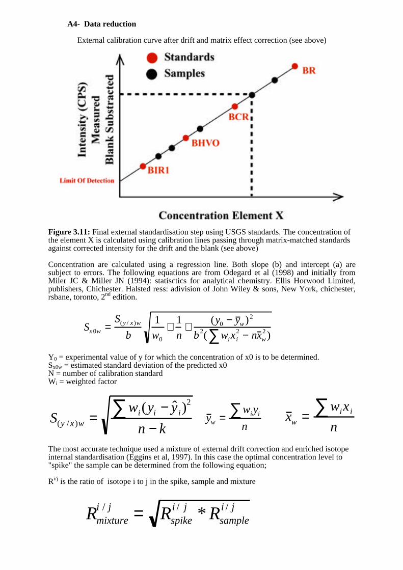
External calibration curve after drift and matrix effect correction (see above)
Figure 3.11: Final external standardisation step using USGS standards. The concentration ofthe element X is calculated using calibration lines passing through matrix-matched standardsagainst corrected intensity for the drift and the blank (see above)
Concentration are calculated using a regression line. Both slope (b) and intercept (a) aresubject to errors. The following equations are from Odegard et al (1998) and initially fromMiler JC & Miller JN (1994): statisctics for analytical chemistry. Ellis Horwood Limited,publishers, Chichester. Halsted ress: adivision of John Wiley & sons, New York, chichester,rsbane, toronto, 2nd edition.
Y0 = experimental value of y for which the concentration of x0 is to be determined.Sx0w = estimated standard deviation of the predicted x0N = number of calibration standardWi = weighted factor
The most accurate technique used a mixture of external drift correction and enriched isotopeinternal standardisation (Eggins et al, 1997). In this case the optimal concentration level to"spike" the sample can be determined from the following equation;
Ri/j is the ratio of isotope i to j in the spike, sample and mixture
Sx 0w =S(y / x )w
b
1
w0
+1
n+
(y0 − y w ) 2
b 2( wix i2 − nx w
2 )∑
S(y / x )w =wi(yi − ˆ y i)
2∑n − k
x w =wix i∑n
y w =wiyi∑n
Rmixturei / j = Rspike
i / j * Rsamplei / j
A5- Applications
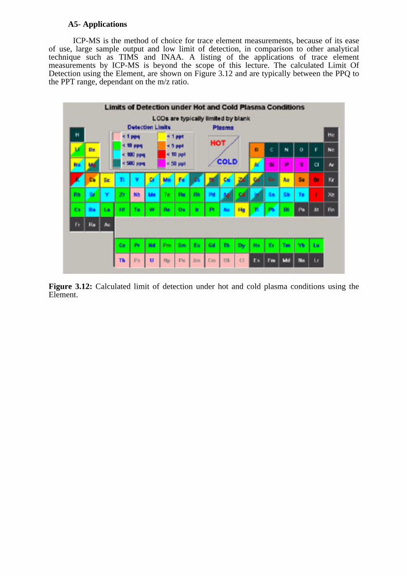
ICP-MS is the method of choice for trace element measurements, because of its easeof use, large sample output and low limit of detection, in comparison to other analyticaltechnique such as TIMS and INAA. A listing of the applications of trace elementmeasurements by ICP-MS is beyond the scope of this lecture. The calculated Limit OfDetection using the Element, are shown on Figure 3.12 and are typically between the PPQ tothe PPT range, dependant on the m/z ratio.
Figure 3.12: Calculated limit of detection under hot and cold plasma conditions using theElement.
B- Sample Introduction System: SOLID
B1- Sample preparation:In general sample preparation is straightforward. Polishing is usually necessary if the
electron microprobe is to be used for internal standardisation before loading the sample intothe sample cell. Because the laser sample cell is not under vacuum, outgazing of the supportmaterial is not a problem.
Powdered samples should be treated in a similar way to XRF analysis and stabilisedeither by
(a) compacting the sample into a pellet with or without a binding agent,or(b) fusing the sample to a borate glass or using a strip heater.
B2- Problems:Several problems are associated with the quantitative analysis of trace elements by
laser ablation ICP-MS:Matrix effects
Dependant on the colour of the mineral and its absorption characteristic of the specificwavelength of the laser ablation system used. Different volume of sample will be ablated.Therefor, two minerals having the same concentration will generate different signal dependanton their physical characteristics (colour, cleavage etc...).
Figure 3.14: Comparison between the ablation of a dark and a light mineral.
Element fractionationSelective removal of some elements and material can be caused by the laser interaction withthe sample, a process termed "elemental fractionation".
Figure 3.15: Fryer et al (1995) have ratioed the signal from the first two minutes over the lasttwo minutes and calculated a fractionation factor while ablating a synthetic glass standard(NIST610). The fractionation intensity seems to follow the Goldschmidt classification ofelements (lithophile, chalcophile and siderophile).
Several process contribute to the fractionation process between element during the ablation:Crater size/depth ratio (Eggins et al, 1998; Mank and Mason, 1999):
At constant laser fluence, the principle parameter, which appears to controlfractionation behaviour, is the aspect ratio of the ablation pit.For the deeper craters the three structural regions of an ablation crater can be defined asfollows:
-Regions A, at the base, The ablation front: The glass appears to have been removedcleanly from the surrounding sample and there is little evidence for the condensation or re-deposition of ablated material. However some very small melt globules (<10 µm) aresometimes seen in this region and the smooth nature of the walls may be due to re-melting bythe plasma following ablation.
-Regions B: The intermediate region: Characterised by thermal cooling cracks on thewalls of the crater. This part of the ablation crater is where particles escape from the ablationfront, some of which are deposited on the walls where they may be re-ablated by reflectedlight and heated by the secondary plasma that penetrates into the ablation crater. Heating inthis region may also lead to volatilisation of elements with the particles that are ablated fromdeeper in the crater.
-Region C: Crater opening: Where large amount of particles redeposition and meltinghave been taken place. Fracturing of the sample is most apparent in this region and may berelated to stress during cooling or recrystallisation of thin molten layers. Deposition aroundthe crater on the surface of the glass sample can be extensive and is dependant upon theamount of material removed during the ablation event, the viscosity or density of the gas inthe sample cell and the dynamics of flow of the gas in the sample chamber.
The model can be applied under all power density, repetition rate and static focusparameters that have been applied in this study. The formation and relative influence of eachstructural unit is controlled by the depth/diameter ratio of the ablation crater.(Mank andMason, 1999). For minimal fractionation it is essential to maintain power density well abovethe ablation threshold giving a crater of similar diameter from the top to the base. Acrater/depth ratio lower than 6 is recommended to reduce the level of fractionation.
Laser wavelength:Ablation mechanisms are influenced by the photon energy of the laser. Shorter
wavelengths offer higher photon energies for bond breaking and ionisation processes. Theablated volume in different matrix will be similar for shorter wavelength in the standard andthe unknown, which limit fractionation effect between the two and make quantification easier(figure 2.24).
Gas mediumSensitivity improvement are expected using mixed gas such as nitrogen. Durrant
(1994) have shown that the addition of about 1% N2 in the coolant gas increase the sensitivityby a factor of 3 for some elements. Addition of about 12% N2 to the cell flow have a similareffect. An improvement by a factor of 5 is also claimed by (Hirata and Nesbitt, 1995) forheavy masses. Moreover, mixed argon-helium atmosphere retards condensation andreprecipitation of ablated material around the excavated crater (Louks, et al., 1995; Eggins etal 1998; Mao et al 1998; Leung et al 1998; Chan et al 1998; Günther and Heinrich 1999) andimprove sensitivity by a factor of 5 for some elements
The manner of deposition of material around the top of the crater is very differentwhen ablating in He with a larger diameter blanket of deposited material. However, thematerial is deposited in a thinner layer of coalesce particles than in the case of the blanketobserved when ablating in Ar.
Particle size and entrainmentParticles of different sizes are entrained into the plasma by the carrier gas for different
laser wavelength. Recent studies have showed that the particle size distribution in the ICP isthe major factor responsible for inter-element fractionation. Therefor other parameter such aspower density or focusing conditions have also an influence.
Interferences
Figure 3.16: Some classic interference mainly due to air entrainment (Si29, P31, Ca44, Fe57,Mn55). The interference are minimal for Ni, Cu and Cr are result mainly from sourcecontamination. Those interference may be reduce by using the medium resolution setting of ahigh resolution magnetic sector ICP.
B3- AcquisitionTHE FASTER - THE BETTER
NB: Dependant on the type of instrument used different terms are used for the same purpose:
Quadrupole Magnetic sectorTotal time required for acquisitionof intensity information of thecomplete list of selected mass
Spectrometersweep time
Total Scan time
Time spent to scan from low tohigh mass
reading Scan time
The sum of several reading Sweep timeTime spent acquiring data at aparticular mass
Dwell time Sample time
Number of acquisition per mass Points per peak(From 1 to 3)
Sample window/number of sample
Time wasted between acquisition Settling time(0.1-2 ms)
Settling time(0.1 to 100 ms with fast
scanning option)
NB: the dwell time is used as the total ablation time with the NewWave laser ablationsoftware.
Tuning and Mass Calibration are the same as for solution analysis
Method
Figure 3.17: Average of 50 scans using a 1 second scan duration which translates to 1000 UVlaser shots at the surface of the sample using a magnetic sector ICP. The typical flat toppedpeak shape produced for La during ablation of NIST 612 (˜37 ppm) is characteristic ofmagnetic sector instruments and should allow the precise measurement of isotope ratios. Theprecision should be higher to that of a quadrupole instrument, which is characterised by amore gaussian peak shape.
Figure 3.18: The efficiency of the method (time spent analysing / total scan time) will bedependant on the number of isotopes and the scanning range. This figure compare theefficiency of an Element1 and a quadrupole instrument while scanning from Ca44 to U238(A) and from La to Hf (for REE measurement in a zircon, B). In the first case the magneticsector instrument reach a maximum of 60% efficiency with a scan duration of 1,2s and with 3points per peak, while the quadrupole reach a higher efficiency using a lower number ofpoints per peak (1) and a much lower scanning time. In this case the quadrupole instrument ismuch more efficient. In the second scenario, both instruments reach similar efficiency using 2points per peak. Since magnetic jumps are slower than electric jumps, magnetic sector willtend to be slower in order to avoid magnet histeresis. Significant improvement has been madeon the second generation of sector field instrument using the fast scanning option (Element2)but quadrupole remain faster and more efficient using classical method involving themeasurement of 30-40 elements from Li to U.
Figure 3.19: Example of a typical laser ablation peak shape (compare with figure 3.15). Thecentre of the peak top is only analysed (4 points per peak in this case), in order to improve thescanning efficiency.
Isotope Mass Mass Mass Magnet Settling Sample Sample Segment Search Integration Detection
Window Range Mass Time Time per Peak Duration Window Window Mode
Figure 3.20: The ‚method‘ window of the Element (compare with the method use for solutionanalysis, figure 3.9). Each elements are analysed using a very small mass window (1%, thevery centre of the peak top define during the mass calibration). The magnet mass shows theposition of the magnet while it rests between jumps. A sample time (time spent on eachchannel of points) has been set at 5 ms. Only one point per peak has been chosen. Thesegment duration will therefor be 5ms for each isotope. All elements has been analysed usingthe Electric Scan (Escan) and in counting mode (major elements such as Si or Ca, in silicates,will be analysed in Analog mode, in order to protect the SEM).
Sequence
Figure 3.21: The ‚sequence‘ window of the Element (compare with the sequence use forsolution analysis, figure 3.10). The sequence (left side) will start with the measurement of anexternal standard such as NIST610, followed by a series of sample before an other externalstandard etc...A specific method and tuning parameter could be associated to each samplesand standards (right side).
NB: the measurement of the blank is a matter of debate: gas blank, gas blank while firing thelaser or blank sample (e.g. high purity quartz).
B4- Data reductionStandardisation (calibration)
Once microparticulate material has been transported by the stream of argon to theplasma, the number of ions which reach the detector depends on (a) the atomic proportions ofthe element in the source mineral, (b) the amount of material removed during ablation, (c) theionisation potential of the element in the plasma, and (d) isotopic abundance. Assuming nofractionation during ablation between volatile and other more refractory elements, it ispossible to overcome these problems using an internal standard (known concentration of oneelement in the unknown using another analytical technique). Electron microprobe analysis isusually used to measure the concentration of the element chosen as the internal standard in theunknown. Calibration can then be achieved by comparing the response for the internalstandard element in a reference material and the unknown. This element response for theinternal standard allows the analyst to apply a correction for other elements included in theselected menu. In order to perform this correction, the geochemist must: (a) assume that theelement response in the unknown is similar to that of the reference material (i.e., bothmatrices are matched); (b) assume that the reference material has a homogeneous traceelement composition and distribution; and (c) correctly choose the internal standard in thematerial analysed (usually a minor isotope of a major element). Once these several operatingparameters has been controlled, a typical analytical sequence comprises; (a) analysis of theargon blank; (b) analysis of the reference material; (c) analysis of the unknown; (d) secondanalysis of the reference material in order to monitor the drift (sensitivity variation of theinstrument through time); (e) analysis of other unknowns.
Figure 3.22: These figures show the evolution of the signal (intensity for several isotopes)through time, while measuring a standard and a sample. A gas blank is usually measured for20-30 seconds, then the laser is firing on the sample and the intensity increase and stabilise(on a log scale). Because of matrix effect, sample having the same concentration will generatedifferent signal, BUT the ratio between elements will stay the same (if there isn’t any inter-element fractionation, see above). The average intensity of the gas blank will be subtracted tothe average intensity of the sample and standard. These intensities will be ratioed to theinternal standard (Ca or Si for silicates for example) and the following equation will be usefor quantification.
Figure 3.23: Equation use for the calculation of the trace element composition using theinternal standardisation technique. I(m, x): Intensity of the element x in the sample orstandard; I(m, Is): Intensity of the internal standard in the sample or standard; Cis:concentration in ppm of the internal standard in the sample; C(m,x)std: concentration of theelement x, in ppm, in the standard; Cis Std: concentration of the internal standard in thestandard.
=I(m, x ) / I(m, Is )[ ]( ) * CIs
( )samp
* C(m, x)( )std
I(m, x) / I(m ,I s )[ ]( )std
* CI s( )std
Limit Of Detection
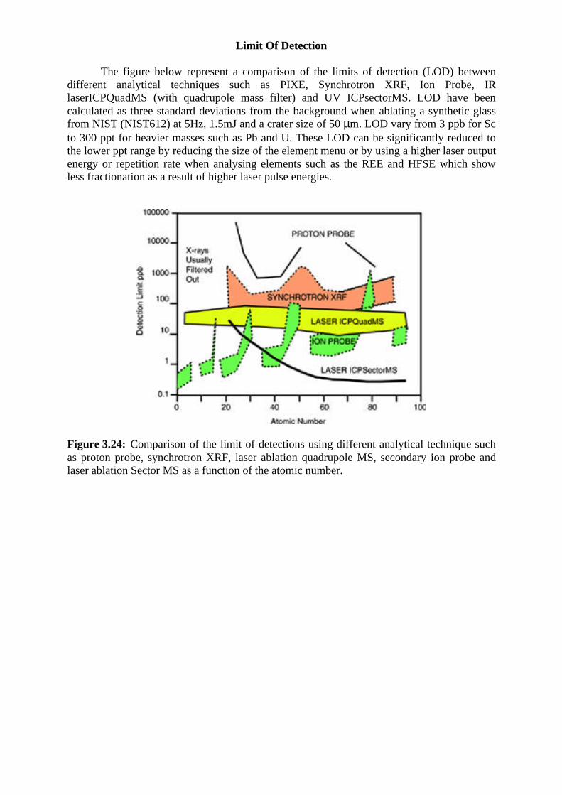
The figure below represent a comparison of the limits of detection (LOD) betweendifferent analytical techniques such as PIXE, Synchrotron XRF, Ion Probe, IRlaserICPQuadMS (with quadrupole mass filter) and UV ICPsectorMS. LOD have beencalculated as three standard deviations from the background when ablating a synthetic glassfrom NIST (NIST612) at 5Hz, 1.5mJ and a crater size of 50 µm. LOD vary from 3 ppb for Scto 300 ppt for heavier masses such as Pb and U. These LOD can be significantly reduced tothe lower ppt range by reducing the size of the element menu or by using a higher laser outputenergy or repetition rate when analysing elements such as the REE and HFSE which showless fractionation as a result of higher laser pulse energies.
Figure 3.24: Comparison of the limit of detections using different analytical technique suchas proton probe, synchrotron XRF, laser ablation quadrupole MS, secondary ion probe andlaser ablation Sector MS as a function of the atomic number.
B5- Standardisation:There are four sets of standard available for quantitative laser ablation analyses of trace
elements. Unfortunately they all have a silica-enriched composition. The compositions ofthese glasses could be found in the appendix.
a- NIST: Standard Reference Material (SRM) of National Institut of Standardsand Technology (NIST): Information on the original manufacturing of these glasses could befound in Hinton (1999). There are mainly made of a mixture if African sand, Diamond alkalicalcium carbonate, Stauffer soda ash, Linde alumina and Olin sodium nitrate. Batches of traceelement were made separately and they were latter on mixed together. They are the mostwidely used for trace element analysis by laser ablation ICP-MS. 4 main types of standardshas been made, having different concentration level and wafer thickness: The sixty oneelements added to the base glass mix have a final concentration of about 450 ppm (NIST 611-610), about 40 ppm (NIST612-613), 1ppm (NIST 614-615) and less than 100 ppb (NIST 616-617). Those glasses are commercially available see NIST website)
b- USGS: United State Geological Survey BCR2G, BHVO2G, BIR1G glasses.They have been produced by re-melting (1600C) approximately 2kg of the original
whole rock powder standard in a 1 litter platinum bowl using a Linderberg heavy duty furnaceequipped with high temperature silicon heating elements. To moderate the oxidisingenvironment of the furnace, 100 ml platinum crucible filled with graphite rods were placebehind and in front of the platinum bowl containing the standards. The platinum bowl wereperiodically tipped to facilitate the mixing of the molten material. After 4 hours, the moltenmaterial was poured out onto a 40 cm3 platinum sheet and allowed to cool. In the pouringprocess the molten material spread across the platinum surface, producing a "pancake" offairly uniform thickness (2cm). Those glasses are available through S. Wilson from theUSGS.c- DHL: A new technique for preparing homogeneous glasses has been developed at the
department of geology of Manchester, using the co-precipitation gel technique(Hamilton & Hopkins, 1995). All component except SiO2 are contained in single solutionas nitrates. About an equal volume of ethanol is stirred into this solution followed by therequired mass of tetraethyl orthosilicate (TEOS). The liquid is vigorously stirred until asingle solution homogeneous liquid results. Concentrated ammonia solution is now addedwhile vigorous stirring continues in order create a gel with the silica and aluminiumhydroxide. The whole content of the beaker should become semi-solid within a fewminutes. 3 main standard have been created (DHL6-7 and 8) with concentrations rangingfrom 1, 70 to 150 ppm. A quartz blank have also been produced using this technique inorder to improve blank correction. A PGE standard has also been produced although it hasa silica rich matrix. They are commercially available by more expensive than the NIST.
- MPI-DING: The last were prepared at the Bayerisches Geoinstitut, Bayreuthfollowing the technique described by (Dingwell et al, 1993). Direct fusion of 50-100g of rockships at temperature about 1400-1600C were produced except for the peridotitic samplewhich was a 5:1 mixture of near pure silica. A thin wall platinum crucible was used to containthe melts. These sample could be contaminated with the ZrO2 insulating boards and theresistive heating elements made of MoSi2, and previous glasses melt from the same container.The glass were held at that temperature for 1 hour and then place in a second furnaceequipped with a viscometer. The melt was stirred at 200 rpm for 12 hours using a Pt80Rh20spindle. The melt was removed and quench by placing the bottom of the Pt crucible intowater. Most of these glasses are homogeneous with the exception of the komatiitic ultamaficglass which shows beautiful olivine spinifex crystallisation feature:
d- Direct fusion in graphite electrode (Odegard, 1999): This technique has beenused to prepare high purity quartz sample as well as synthetic rutile composition. The fusiontime is about 1mn. This technique is fast and cost effective however the presence of gasbubble and some heterogeneity remain.