University of Connecticut OpenCommons@UConn Economics Working Papers Department of Economics April 2005 A Simple Model of Credit Rationing with Information Externalities Akm Rezaul Hossain University of Connecticut Follow this and additional works at: hps://opencommons.uconn.edu/econ_wpapers Recommended Citation Hossain, Akm Rezaul, "A Simple Model of Credit Rationing with Information Externalities" (2005). Economics Working Papers. 200511. hps://opencommons.uconn.edu/econ_wpapers/200511
Transcript
University of ConnecticutOpenCommons@UConn
Economics Working Papers Department of Economics
April 2005
A Simple Model of Credit Rationing withInformation ExternalitiesAkm Rezaul HossainUniversity of Connecticut
Follow this and additional works at: https://opencommons.uconn.edu/econ_wpapers
Recommended CitationHossain, Akm Rezaul, "A Simple Model of Credit Rationing with Information Externalities" (2005). Economics Working Papers.200511.https://opencommons.uconn.edu/econ_wpapers/200511
AbstractCredit-rationing model similar to Stiglitz and Weiss [1981] is combined with
the information externality model of Lang and Nakamura [1993] to examine theproperties of mortgage markets characterized by both adverse selection and infor-mation externalities. In a credit-rationing model, additional information increaseslenders ability to distinguish risks, which leads to increased supply of credit. Ac-cording to Lang and Nakamura, larger supply of credit leads to additional marketactivities and therefore, greater information. The combination of these two propo-sitions leads to a general equilibrium model. This paper describes properties ofthis general equilibrium model. The paper provides another sufficient conditionin which credit rationing falls with information. In that, external information im-proves the accuracy of equity-risk assessments of properties, which reduces creditrationing. Contrary to intuition, this increased accuracy raises the mortgage in-terest rate. This allows clarifying the trade offs associated with reduced creditrationing and the quality of applicant pool.
Journal of Economic Literature Classification: C62, R31, R51.
Keywords: Credit rationing, Information Externalities, Adverse selection,Mortgage underwriting.
3
Introduction
Stiglitz and Weiss (S-W) [1981] show how credit rationing2 may occur as a result
of adverse selection in the credit markets. Using Rothschild and Stiglitz [1976] approach
to analyze information asymmetry, Brueckner [2000] also shows a form of credit
rationing that emerges because of adverse selection in the mortgage markets3. In this
paper, we consider a S-W type credit-rationing model and incorporate information
externalities that are caused by the level of market activities. Specifically, the Lang and
Nakamura (L-N) [1993] hypothesis concerning information externalities in the mortgage
market is incorporated into a traditional credit-rationing model. Although the L-N model
describes externalities that are specific to mortgage market, the model introduced in this
paper is applicable to other markets characterized by adverse selection and information
externalities, such as consumer lending, employment and insurance markets.
According to the L-N model, market activities measured by total loan volume in a
neighborhood reduce the error4 associated with the appraised value of properties.
Improved assessments of the properties allow lenders to distinguish observable risks,
which increases lenders’ profit at all interest rate, leading to increased supply of loans.
Although certain lenders are responsible for generating this information (more accurate
appraisals), every lender benefits from it. The majority of the empirical studies [Calem
1996, Ling and Wachter 1998, Avery et. al. 1999, Harrison 2001] find evidence
2 S-W [1981] defines credit-rationing as a situation where, (a) among observationally equivalent credit applicants some receive credit and others do not or (b) there are identifiable groups of applicants who, with a given supply of credit, are unable to obtain loans at any interest rate, even though with a larger supply of credit they would. 3 Using a model of mortgage default, Brueckner [2000] shows that in the equilibrium safe borrowers cannot obtain the large and high-LTV mortgages at a fair price because such mortgages are not offered in the market. The reason lenders do not offer such mortgages is that they would attract risky borrowers resulting loss to the lenders. 4 This is the divergence between the actual market value and the assessed value of the property.
4
supporting information externalities in the context of mortgage market by showing
significant effect of neighborhood-specific total loan volume on underwriting decision.5
The L-N type information generation process has important implications for the
credit-rationing model. In a credit-rationing model, additional information that increases
lenders’ ability to distinguish risks leads to increased supply of credit. On the other hand,
according to Lang and Nakamura, larger supply of credit leads to additional market
activities and therefore, greater information. The combination of these two propositions
leads to a general equilibrium model. This paper describes properties of this general
equilibrium model.
Since the seminal paper by S-W, credit rationing remained an active area of
research in both theoretical and empirical fronts. In a typical S-W model, credit rationing
is a consequence of adverse selection, or lenders’ inability to observe and separate the
low- and high-risk borrowers. One of the ways to mitigate credit rationing is to design a
mechanism that allow lenders to separate the risk types, or provide borrowers with
incentives to self-select according to risk types. Numerous theoretical papers have looked
at the existence and equilibrium properties in the credit-rationing model. Bester [1985]
shows that active screening by lenders in a credit-rationing model can eliminate rationing
in the market. Besanko and Thakor [1987] model shows that by offering different types
of credit contract, lenders may induce borrowers to self-select across their risk types and
this can eliminate credit rationing. In a similar fashion, Calem and Stutzer [1995] design
two types of credit contract for two risk types and use down payment requirements to
separate the risk types. In Ben Shahar and Feldman [2001], two types of contracts for two
5 After controlling for neighborhood fixed effects, Hossain and Ross [2004], however, finds no evidence of the effect of total application volume on mortgage underwriting.
5
risk types and divergent loan terms allow lenders to separate borrowers across the risk
types. More recently, in the context of subprime lending Cutts and Van Order [2004]
paper shows how divergent costs of rejection provides incentive to borrowers to reveal
information about their types. This paper combines the S-W type credit-rationing model
with the L-N type information externalities. In doing so, it explicitly incorporates
information externalities into credit-rationing model and illustrates an additional
mechanism by which credit rationing may be reduced or eliminated.
The S-W model shows how credit rationing emerges in the presence of adverse
selection. This paper extends the S-W model in another important way. In that, the paper
solves the general equilibrium levels of credit rationing and information level
simultaneously and provides theoretical insights that cannot be obtained by the S-W
credit rationing or the L-N type information externalities models alone. The associated
comparative static results provide important implications for policies relating to credit
markets. The paper highlights some of these implications. Finally, the paper suggests that
in a general equilibrium model an increase in loan volume due to the L-N type
information externalities may be mitigated by the resulting increase in the interest rate in
the credit-rationing model. Consequently, empirical research may find reduced effect of
the L-N type information externalities.
6
The paper is organized in six sections. Section II describes the behavior of the borrowers
or the demanders of mortgage credits. Section III describes the loan supply decision of
lenders in the presence of adverse selection. The credit rationing equilibrium is derived in
section IV. Section V derives the equilibrium results by incorporating information
externalities into credit-rationing model. Finally section VI, summarizes the findings,
discusses several key implications of these findings and points out some of the possible
extensions to the paper.
7
II. The Borrowers
In this simple, stylized model of credit markets, there are two types of borrowers:
the low-risk and the high-risk borrowers. These borrowers are event-defaulter in the
sense that exogenous events like death, divorce or loss of employment generate an
unexpected shock in their consumption or income streams leading to default. Although
borrowers are event-defaulter, one of the crucial assumptions of our model is that the
borrowers possess better information about their ability and intention to cope with the
unexpected events than the lenders. This is the source of adverse selection in this model.
In the event of default, lenders repossess the property and attempt to recover their
investments through foreclosure, but the borrowers face no future monetary costs. Due to
information asymmetry and costless default, the high-risk borrowers always demand
more loans than the low risk borrowers at all possible interest rates. In the event of
unexpected shock, the low-risk borrowers continue to fulfill their mortgage obligations.
However, in the similar event high-risk borrowers default on their mortgage and fail to
make their contractual payments.
Demand Functions A general downward sloping demand function for the low- and high-
risk borrowers can be expressed as follows:
Low-risk borrowers: DL = � [Ld (r) - �] when r < rl (1)
0 when r � rl
High-risk borrowers: DH = � [Ld (r) + �] when r < rh (2)
0 when r � rh
8
Where,
L�d (r) < 0 (3)
� is a parameter that changes the total demand for loans without affecting the
relative share of demand6 by two types of borrowers.
� is a parameter that changes the relative share of the loan demand by two types
without affecting the total market demand.
For simplicity, the slopes are assumed equal so that DH always lies above DL. The
parameter � in the demand function of high-risk borrowers represents a shift parameter
that captures the difference in quantity of loan demanded between two types of
borrowers. We assumed that this difference is invariant with interest rate until low-risk
borrowers exit the market at the interest rate rL. The basic results of this paper hold even
if demand functions (DL and DH) have unequal slopes or the parameter � varied with
interest rate, as long as DH always lies above DL.
In the figure 1, we have demand functions for low- and high-risk borrowers, and
the market demand function for mortgage credit (DM). The low-risk borrowers exit the
market at the interest rate (rL) when high-risk borrowers still demand for credit. At rH,
high-risk borrowers demand no credit as well. The market demand function (DM) can be
obtained by vertically summing demand functions of the low-risk (DL) and high-risk (DH)
borrowers as expressed in the equation 5.
6 Note the share of loan demand by the low- and high-risk borrowers in the relevant range are �L(r)= [Ld (r)- �]/2.Ld (r) and �H(r)= [Ld (r)+ �]/2.Ld (r) respectively. This shares the derived in the following section in equation (9) and (10).
9
Figure 1
The Demand Curves
L(r) DM
DH
DL
rL rH r Figure 1 In the figure, interest rate (r) is the independent variable and shown in the horizontal axis unlike usual market demand curve where price is on the vertical axis. DL, DH and DM represent demand function for the low-risk borrowers, the high-risk borrowers and the market demand respectively. At interest rate rL, low-risk borrowers exit the market.
The market demand function, therefore, has both the pooling and separating
components. In the pooling component, both low-risk and high-risk borrowers apply for
loans. In the separating component, however, only the high-risk borrowers apply.
DM = 2.�.Ld (r) for 0 � r < rl [Pooling component] (5)
�.[Ld (r) + �] for rl � r < rh [Separating component]
0 for r � rh
10
As will be discussed later, there are two types of property: the low- and high-
equity risk properties. Since all defaults are resulted from unexpected events, defaults are
assumed to be unaffected by the equity risk of the property or the dwelling attributes.
Therefore, the probability of default is same for both risk types regardless of the type of
property.
III. The Lenders
This section derives the loan supply as function of interest rate for a
representative lender. In the model, all lenders are risk-neutral who maximize expected
profit. Assuming an exogenously given market for commercial investments besides the
mortgage market and the no arbitrage condition in the rate of returns for competing
investments, we show that the loan supply function is directly related to the expected rate
of return function. Next, we will derive the rate of return function for both pooling and
separating case.
Rate of Return Function �(r,c):
In the event of unexpected shock, the high-risk borrowers are more likely to
default. Therefore, on the average high-risk borrowers provides a rate of return less than
that of low-risk borrowers at all interest rates. We assume the following simple rate of
return functions for two types of borrowers:
Rate of return of low-risk borrowers is,
�L(r,c) = �(r,c) = r-c (6)
11
Rate of return of high-risk borrowers is,
�H(r,c, �) = �(r,c) - � = r - c – � (7)
Where,
r = Interest rate, where r > 0
c = Cost of fund rate, where c > 0
� is a positive constant. Therefore, �L(r) > �H(r) for all r
The parameter � in the rate of return function of high-risk borrowers represents
the loss due to inherent risk associated with the borrower type. For simplicity, we assume
that the loss of rate of return does not vary with the interest rate. The rate of return
functions for the low- and high-risk borrowers are in the figure below.
12
Figure 2
Rate of Return Functions
�(r)
�L(r,c) = r - c
�H(r,c,�) = r- c - �
c c+ � r
- c
- (c+ �)
Figure 2 shows the rate of return functions �L(r,c) and �H(r,c, �) associated with the low- and high-risk borrowers respectively.
Expected Pooled Rate of Return
From the specific form of the demand function, it is possible to derive the
expected pooled rate of return function. By definition, the expected pooled rate of return
takes the following form.
�pool(r) = �L(r) . �L(r) + �H(r) . [1- �L(r)]
Here,
�L(r) = Proportion or share of the low-risk borrowers in the pool at interest rate r.
See equation 9 for the specific expression of this share.
13
The pooled rate of return is the expected rate of return. In that sense, �L(r) will be
interpreted as the probability that any given borrower in the pool is a low risk type.
Pooled rate of return can be simplified as follows,
�pool(r) = �L(r) . �L(r) + �H(r) . �H(r)
= �L(r) . �L(r) + [�L(r) - �] �H(r)
= �L(r) [ �L(r) + �H(r)]- � .�H(r)
= �L(r) - � .�H(r) (8)
From the demand function, we can write the specific form of �L(r) and �H(r) as a
function of the interest rate r as follows,
�L(r) = Proportion of low-risk borrowers in the pool when interest rate is r
= Number of low-risk borrowers at r/Total number borrowers at r
= [Ld (r)- � ]/2.Ld (r) (9)
From the construction of the demand function, note that the proportion or the
share of low risk borrowers is affected by �, but does not depend on parameter � in the
demand function.
Proposition 1. Pool quality falls with the interest rate.
Proof:
We take first derivative of �L with respect to r. We find,
��l(r) = �.L�d (r)/ 2.[Ld (r)]2 < 0
Since, � > 0, L�d (r) < 0 and the denominator is positive, ��L(r) < 0 #
14
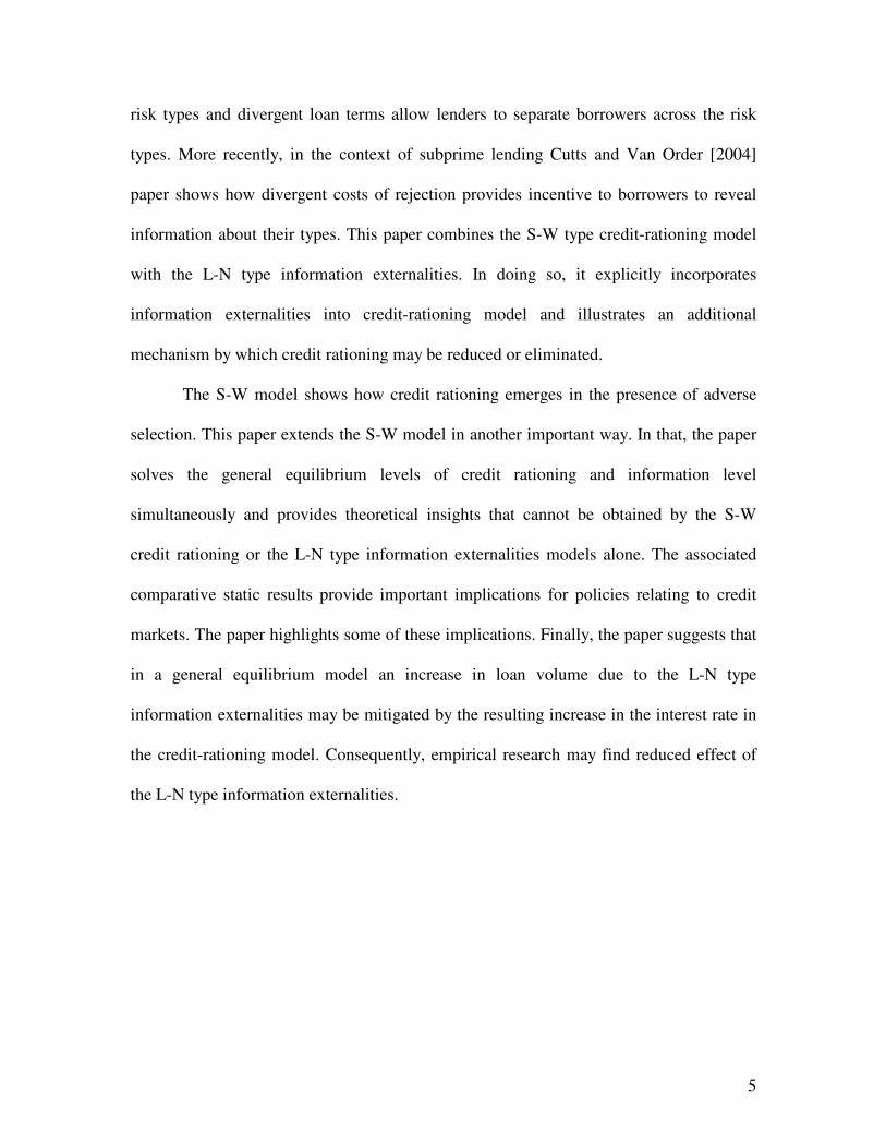
The market rate of return �m(r) is composed of both the pooling and separating
components. In the pooling rate of return, both types of borrowers apply for loans. In the
separating components only the high-risk borrowers stays in the market. Market rate of
return can be expressed as:
�m(r) = �pool(r) = �L(r) - � .�H(r) when r < rL [Pooling rate of return] (10)
�L(r) = �L(r) - � when r � rL [Separating rate of return]
Conditions for Maximum Pooled Rate of Return
The First Order Condition (F.O.C.) and the Second Order Condition (S.O.C.) for
pooled rate of return to reach its maximum is given by the following equations.
F.O.C.:
��pool(r) = �L�(r,c) - � .�H� (r) = 0 (11)
S.O.C.:
���pool(r) = �L�� (r,c) - �.�H�� (r) < 0
�l��(r,c) < �.�h�� (r) (12)
Conditions in the equations 11 and 12 ensure the existence of an r* at which
pooled rate of return is maximum7. In the figure 3, on the upper panel functions �L(r) and
�.�L(r) are drawn. On the lower panel, the market rate of return function �m(r) is drawn,
which is the difference between �L(r) and �.�H(r) functions when r < rL and the difference
between �L(r) and � when r � rL [see equation 10]. In the upper panel, �L(r) and �.�H(r)
functions are drawn as function of interest rate. Note �H(r)=1 when r � rL. Therefore,
�.�h(r) = � when r � rL. In the lower panel, market rate of return �m(r) is drawn, which is 7 Later in the paper, we show that under certain conditions the interest rate at which pooled rate of return is maximized, or r* is also the equilibrium credit rationing interest rate.
15
the difference between �L(r) and �.�H(r). The market rate of return function or �m(r) has
two components: the pooling and the separating component. At interest rate rL, low-risk
borrowers exit the market. Therefore, when r < rL, �m(r) is equal to pooled rate of return,
or �pool(r) as shown by the dark solid line in the lower panel. �m(r), however, is equal to
the rate of return of the high-risk borrowers, or �H(r) when r � rL as shown by the dotted
line.
The lower panel of figure 3 shows the humped-shaped market rate of return
function, which is a non-monotonic function of the interest rate. This non-monotonecity
is the consequence of adverse selection and a key feature of the S-W type credit-rationing
model. The rate of return increases with interest rate, ceteris paribus. We call this the
price effect of interest rate. Due to adverse selection, however, the low-risk borrowers
disproportionately drop out of the applicant pool. We call this as the sorting effect of
interest rate. The rate of return at the interest rate r* reflects a point at which the marginal
change in the price effect is equal to the marginal change in the sorting effect. Interest
rates above the r*, sorting effect overwhelms the price effect and the rate of return starts
falling until rL. Above the rL, only the high-risk borrowers stay in the pool. Therefore, no
sorting effect exists and the interest rate keeps rising due to price effect.
16
Figure 3
The Market Rate of Return Function, or �m(r)
�l(r) and �.�h(r)
�l(r)
�.�h(r)
�
c r* rL r
- c
�m(r)
Pooling Component Separating Component
�h = �l(r)- �
�pool = �l(r) - �.�h(r)
r* rL r
Figure 3 in the upper panel �L(r) and �.�H(r) is drawn as function of interest rate. In the lower panel, the market rate of return �m(r) is drawn which is the difference between �L(r) and �.�H(r). Note, the �H(r) = 1 when r � rL, therefore �.�H(r)= �.
17
Market Supply Function Sm(r)
In this subsection, we show that the loan supply function is a monotonic function
of the market rate of return. More Specifically, the loan supply function, or LS(r) can be
expressed as a function of interest rate through rate of return as below.
Sm = Ls(�m(r)) Where Ls� > 0 (13)
Although rate of return, �m(r) is a non-monotonic function of interest rate, r
[Hump in the lower panel of Figure 3], the loan supply, or Ls(�m) is a monotonic function
of rate of return, or �m. By showing this monotonic relation, we know that the shape of
market supply function (Sm) will be identical to the shape of the rate of return function
(�m).
We will refer to all commercial projects except the mortgage loan as ‘commercial
projects’ and assume that an exogenously given total loanable credit is distributed among
the mortgage market and the market for all other commercial projects in the following
way:
Ls=Lsm+Lsc (14)
Where,
Ls is the total exogenous supply of loans in the economy.
Lsm is the loan supplied to the mortgage market.
Lsc is the loans supplied to the market for other commercial projects.
18
We also assume that the supply of commercial projects is characterized by
diminishing marginal rate of return. Accordingly, the marginal rate of return on the funds
invested in commercial projects declines with Lsc as shown in the figure 4 below. In the
figure, �com shows the relationship between loan supply and rate of return in the market
for commercial projects.
Figure 4
The Rate of Return Function for Commercial Projects
�c
�com
�m2
�m1
�min
c k2 k1 Ls Lsc
Lsc Lsm
Figure 4 shows the rate of return as a function of loan supply in the market for commercial projects besides the mortgage loans.
In equilibrium, rate of return in the two markets must be equal. Therefore, if the
rate of return in the mortgage market is �m1, Lsc will be equal to k1 and Lsm = Lsc – k1. A
higher rate in the mortgage market, such as �m2 will decrease Lsc and lead to an increase
in Lsm.
19
Specifically, lets recall equation 14, the distribution of loan supply across two
markets,
Ls = Lsm(�) + Lsc(�)
Rearranging the terms,
Lsm(�) = Ls - Lsc(�)
Taking first derivative with respect to �, we get,
L�sm(�) = - L�sc(�)
Due to diminishing marginal rate of return in the market for commercial projects,
L�sc(�) < 0. Therefore, L�sm(�) >0 for all �. Therefore the loan supply in the mortgage
market is a monotonic function of rate of return in the mortgage market. The supply
function can be expressed as follows,
Sm(r) = Lsm(�m(r)), where Ls� (�m) > 0
= Lsm(�pool(r)) when r < rL [Pooling component] (15)
Lsm(�H(r)) when r � rL [Separating component]
IV. Credit Rationing Equilibrium
In the figure 5, market demand, Dm(r) and supply, Sm(r) intersects at rm. Lender,
however, will not offer this interest rate to borrowers. Instead, lender will offer the
interest rate, r* at which the pool rate of return is maximized. Beyond r*, as the interest
rate goes up, the rate of return associated with low-risk borrowers, �L(r) rises. The loss of
rate of return due to increased proportion of high-risk borrower �.�H(r), however,
overwhelms this rise causing the net pooled rate of return, �L(r) - �.�H(r) to fall.
20
Figure 5
Credit Rationing Equilibrium
Sm and Dm
Credit Sm
Rationing
Dm
r* rl rm r
Figure 5 The market demand (Dm) and supply (Sm) function are drawn. The supply curve has the same shape as rate of return function. The demand function has a kink at rL where low-risk borrowers drop out of the market.
At the pooled credit rationing equilibrium, the interest rate is r*. The number of
loans demanded is,
Dm(r*) = 2.�.Ld (r*).
The number of loans supplied is,
Sm(r*) = Ls(�pool(r*))
= Ls(�(r*) - � .�H(r*))
21
Therefore, the equilibrium level of credit rationing is,
CR(r*) = Dm(r*) - Sm(r*)
= 2.�. Ld (r*) - Ls(�(r*) - � .�H(r*)) (16)
Condition for the Existence of the Pooled Credit Rationing Equilibrium
The interest rate r* characterizes a pooled credit rationing equilibrium at which
lenders pooled rate of return is maximized. The credit rationing equilibrium that occurs
when both low- and high-risk borrowers apply for loans have the following necessary and
sufficient conditions.
Necessary Condition The necessary condition for the pooled credit rationing equilibrium
to exist is,
��pool(r*) = 0 such that r* < rm (17)
Sufficient Condition The sufficient condition for the pooled credit rationing equilibrium
to exist is,
Dm(r*) > Sm(r*) and �m(r*) > �m(rm) (18)
Appendix 1 considers several situations in which the necessary or the sufficient
conditions are violated.
V. Credit Rationing Equilibrium with Information Externalities
This section introduces the L-N type information externalities into the credit-
rationing model developed thus far and finds the equilibrium properties of the model
characterized both by credit rationing and information externalities. Specifically, the
section describes how the effects of the increased mortgage market activities and
22
consequent improvement of the appraised value are incorporated into a traditional credit-
rationing model. This section introduces the effect of heterogeneous property types on the
rate of return function. The properties of the equilibrium including the existence, stability
and comparative statistics of some key parameters are also described in this section.
Loss of Rate of Return Function (�) and Property Types
We have assumed that the loss of rate of return due to high-risk borrowers, or � is
a constant that does not change with interest rate. Although we continue to maintain this
assumption, in this section, we specify how � might vary across heterogeneous property
types. This is described in the diagram below. In the diagram, there are two types of
borrowers: low- and high-risk borrowers, and two types of properties: low- and high-
equity risk properties. Each borrower type can purchase either a low-equity risk or a
high-equity risk property. The probability of a low- and high-risk borrower to purchase a
low-equity risk property is PL,L and PH,L respectively. However, the probabilities of
default for low- and high-risk borrowers are PL and PH respectively regardless of the
equity risk of the property8.
We will continue to normalize the loss of rate of return for low-risk borrowers as
zero. A positive loss of the rate of return for the low risk borrowers does not change the
fundamental results of this paper. In the diagram, we assume that the loss of rate of return
associated with the high-risk borrowers, or � varies with the property types. Specifically,
8 This is consistent with the earlier assumption that borrowers are event defaulters rather than ruthless defaulters. The probability of default is not affected by property types for both borrower types of borrowers. In other word, we assume that there is no correlation between borrower types and the property types. This paper does not model how property risk may affect default probability or how borrowers may be sorted across property types according to their risk types.
23
the loss is �L when high-risk borrower purchases a low-equity risk property and �H when
high-risk borrower purchases and high-equity risk property and �H> �L.
Figure 6
Model Diagram
Borrower Type: Low Risk High Risk
Property Type: Low High Low High Equity Equity Equity Equity Risk Risk Risk Risk
Probability of outcome: [PL,L] [1-PL,L] [P H,L] [1-P H,L]
Probability of default: PL PL PH PH
Loss of Rate of Return: 0 0 �L �H
Figure 6 shows the borrowers and the property types with the associated probabilities of outcomes and defaults. The loss of rate of return with low risk borrowers is normalized to be zero regardless of property types. Loss of rate of return with high-risk borrowers, however, is �L when they purchase a low-equity risk property and �H when they purchase a high-equity risk property. Here, �H> �L.
24
Prediction about the Property Equity Risk
Lenders form their prediction about the equity risk associated with the property
under transaction by observing certain neighborhood- and property-specific attributes or
signals that are obtained through the appraisal process. With the increased market
activities, as the number of transaction in the neighborhood increases, the quality of the
appraisals in the neighborhood improves, which makes the signal more accurate. The
formation of prediction about the equity risk associated with the properties can be
expressed as follows:
L = Probability [The property is of low equity risk (LER) | property is actually LER,
information level I]
We also assume,
dL / dI > 0 (19)
This assumption simply means that higher level of information through increased
market activity increases the accuracy of the prediction about the equity risk associated
with the property. The L-N [1993] paper shows that increased external information
captured by the neighborhood level total application volume reduces the appraisal error
(variance) associated with the housing property in the neighborhood. This assumption is
similar in spirit to this L-N finding. The expected loss of the rate of return associated with
the high-risk borrowers can be expressed as a function of information as follows,
�(I) = �L* L(I) + �H* [1-L (I)]
= �H – (�H – �L)* L(I)
= �H – * L(I) where = (�H – �L) (20)
25
Proposition 2: An increase in the level of available information has the following effects:
(a) It reduces loss of rate of return �(I) associated with the high risk borrowers
(b) It increases pooled rate of return �pool(r) at any given interest rate and
Proof:
(a) Taking first derivative of �(I) in equation 20 w.r.t. I,
��(I) = – * �L(I)
Since d �L / d I > 0,
��(I) < 0
This implies that information reduces loss of rate of return �(I) associated with the high
risk borrowers.
(b) Recall the pooled rate of return in equation 11,
�pool(r,I) = �L(r) – �(I).�H(r)
Taking first derivative of �pool(r,I) w.r.t. I,
��pool(r,I) = �L(r) - �� (I).�H(r)
Since ��(I) < 0,
��pool(r,I)>0
This implies that information increases pooled rate of return, or �pool(r) at all interest
rates #
26
Effect of Information on the Equilibrium Credit Rationing Interest Rate (r*)
It is crucial to know if the equilibrium interest rate charged by the lender changes
with information. In other words, we need to know if the peak of supply function shifts
horizontally with information. This section shows that the equilibrium interest rate (r*)
goes up with information. This is a fundamental result of this paper affecting the general
equilibrium properties very significantly.
Proposition 3: Increased information has two effects:
(a) It increases the equilibrium credit rationing interest rate (r*).
(b) It reduces the extent credit rationing in the market.
Proof:
The equilibrium interest rate r* is defined by the First Order Condition that maximizes
the pooled rate of return function. This is,
��pool(r*) = 0
or, �L� (r*) - � (I).�H� (r*) = 0
This can be rewritten as,
G(r*,I) = �L� (r*) - � (I).�H� (r*) = 0
By invoking Implicit Function Theorem,
d r*/ d I = - G �I / G �r
= ��(I).�H� (r*) / [�L�� (r*) - � (I).�H�� (r*)]
Since ��(I) <0 [proposition 2], �H� (r)> 0 [proposition 1] and the denominator is
negative by the Second Order Condition [Equation 13] of the rate of return
maximization,
d r*/ d I > 0 (21)
27
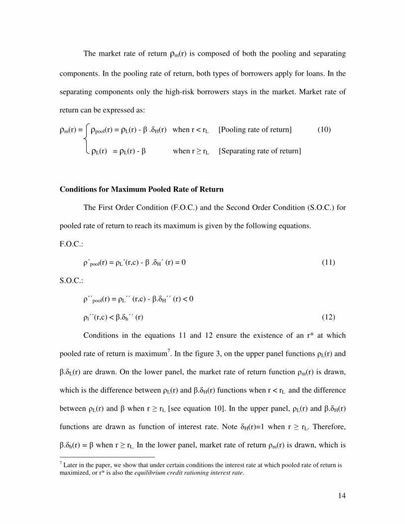
(b) Since loan supply is a direct function of rate of return and the rate of return increases
with information at all interest rates, it is straightforward to show that credit rationing
falls with information.
Equilibrium credit rationing is,
CR(r*,I) = Dm(r*) - Sm(r*,I)
= Dm(r*) – LS(�pool(r*,I ))
Taking first derivative of CR(r*,I) w.r.t. I, we get,
CR� (r*,I) = – LS� (�pool)* ��pool (r,I )
Since LS� (�M)>0 and ��pool (r,I )> 0,
CR� (r*,I)<0
This implies that credit rationing falls with information #
The proposition 2 and 3 are shown graphically in the figure 7 below. In the figure,
market demand (Dm) and supply (Sm) functions are drawn. The supply curve is drawn for
two different information levels (I1 and I2), where I2 > I1. Initially, when information level
is I1, credit rationing equilibrium occurs at r1* satisfying the necessary and the sufficient
conditions.
28
Figure 7
Effect of Information on Credit Rationing Equilibrium Interest Rate
Dm, Sm, �m(r)
Credit-
Rationing Sm(I2)
. �m(r1*) Sm(I1)
�m(rm)
Dm
r1min r1* r2* rL rm r
Figure 7 shows the effect of information on equilibrium interest rate under credit rationing.
According to proposition 2, as the level of information rises from I1 to I2, loss of
rate of return, or �(I) falls and therefore, market rate of return shifts up. Sine the supply
curve is a monotonic transformation of the rate of return function, the supply curve shifts
up to Sm(I2). This is shown by the dotted line in the figure. The rise in the supply curve
reduces the extent of credit rationing in the market. According to proposition 3, however,
the equilibrium credit rationing interest rate shifts horizontally from r1* to r2* in response
to the change in information.
29
The proposition 3 implies that the equilibrium interest rate in the market goes up
with information. This apparently counter intuitive result will form the basis for the rest
of the paper. Intuitively, lenders pooled rate of return function, or �pool(r) = �L(r) –
�(I).�H(r) consists of two components: �L(r) and �(I).�H(r). While the former enhances
lender’s rate of return, the latter has the effect of reducing rate of return. The former
expresses the price effect of interest rate; as the price of credit increases, lender’s rate of
return increases. The latter expresses the sorting behavior of borrowers; as the interest
rate goes up, pool quality falls by increasing the proportion of high-risk borrowers. As the
information level increases, loss of rate of return, or �(I) falls. This allows lenders to
increase rate of return by raising interest rates.
The L-N Hypothesis
According to the L-N hypothesis, market activities generate public information.
Specifically, the degree of activities in the neighborhood mortgage market measured by
the total number transactions increases the overall accuracy of the appraisal value of the
properties in the neighborhood. Increased accuracy of the assessment is the nature of the
new information, which is available to all lenders operating in the neighborhood
regardless of any individual lender’s market activity9. The L-N type information
externalities can be introduced into the credit-rationing model using a proxy that captures
9 Note that the appraisals of a given lender need not to be public information for the L-N type information externalities. The number of appraisals performed in the neighborhood is just a proxy for relevant market activities, and captures the level of accuracy associated with the appraisals. Better assessments in an active neighborhood help all lenders and from this consideration, market activities create is public information and information externalities. For example, appraisals in a neighborhood with sparse activities are not likely to approximate true market value very closely and more likely to exhibit higher variance. The total application volume used in the L-N model perfectly captures the appraisal activities, since every mortgage application triggers an appraisal.
30
the neighborhood-specific market activities. The L-N paper suggests the use of
application volume. Since every loan application triggers an appraisal of the property that
contributes to the improvement of the overall accuracy of the assessment, application
volume can be a reasonable proxy for relevant market activities.
Externalities Through Demand: Whenever an applicant demands for mortgage credit, it
initiates an appraisal of the property under transaction. Since the appraisals are conducted
regardless of the loan supply decision, the appraisals are associated with the loan demand
and do not depend on whether the loan is actually supplied. The appraisal activities
improve the quality of assessment by reducing the error between appraised value and
actual market value of the properties in the neighborhood. The quality assessment, in
turn, affects the underwriting decision all lenders by inducing them to make more loans.
In the through demand approach, appraisal activities that produce new information are
measured by the demand for loans, or the total number of application volume10.
Following the L-N hypothesis, in this paper we incorporate information
externalities into the credit-rationing model through demand. In that, any given level of
loan demand and consequent appraisal activities generates a particular level of
information through the L-N process. This information, however, affects lenders’ ability
10 According to ‘Externalities Through Supply’, actual loan transactions, subsequent servicing of the loans and default experience produce information relevant for underwriting, and help in generating more loans. Although a part of this information is private, and therefore affects the loan supply decision of the originating lenders (causes no externalities), a part of it can be public. For example, default experience of one lender can reach to public domain through foreclosures. In addition, a limited data with the credit scoring company is public and can be geocoded to the neighborhood level to understand the loan performance in the neighborhood. As the number of actual loan supplied in the neighborhood rises, accuracy of the both private and public information about the neighborhood increases. Although total number of loan supplied in the neighborhood does not capture the L-N type information externalities, this can be a measure of total neighborhood-specific information (both internal and external) available to lenders.
31
to predict about the equity risks associated with the properties in the neighborhood. This
improved ability to predict reduces loss associated with high-risk borrowers and affects
the equilibrium interest rate offered in the market characterized by credit rationing model.
The equilibrium interest rate, in turn, affects the number of loan demanded by the
borrowers. In equilibrium, information generated by the L-N hypothesis must be
consistent with the loan volume demanded. This equilibrium solution can be expressed
by equations (A) and (B) below:
Equation (A) The L-N Process: I* = I (LD*)
Here, the loan demand produces information. This can be shown by the figure 8
below. In the figure, loan demand LD produces information I. We assume that all lenders
possess a minimum level of information, or IMIN and a maximum level of feasible
information, or IMAX that can be obtained about the properties and its attributes. This
information rises monotonically with the loan demand at a diminishing rate.
32
Figure 8
The L-N Process in the I-LD Space
I
IMAX
IMIN
LD
Figure 8 shows the relationship between loan demand and level of information available about the equity risk of the neighborhood properties.
Equation (B) The Credit Rationing Model: LD* = L ( r* ( I* ) )
The Equation (B) characterizes the credit-rationing model described in the section
IV. In the model, information affects equilibrium interest rate, which affects the loan
demand through the market demand function. We will show the equilibrium solution
using a graphical approach. Next, we will solve for the analytical solutions for the
equilibrium loan demand LD* and equilibrium level of information I*, and perform
several comparative static to understand the properties of this equilibrium.
Graphical Approach
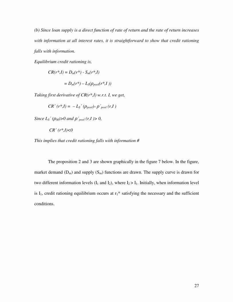
In the graphical approach, we consider three relationships in four quadrants of the
Cartesian co-ordinate system. These three relationships are:
33
1. Relationship between loan demand (LD) and information level (I) represented by
L-N Curve.
2. Relationship between information level (I) and the equilibrium interest rate (r*)
represented by Equilibrium Interest Rate Curve.
3. Relationship between the equilibrium interest rate (r) and the loan demand (DM)
represented by Demand Curve.
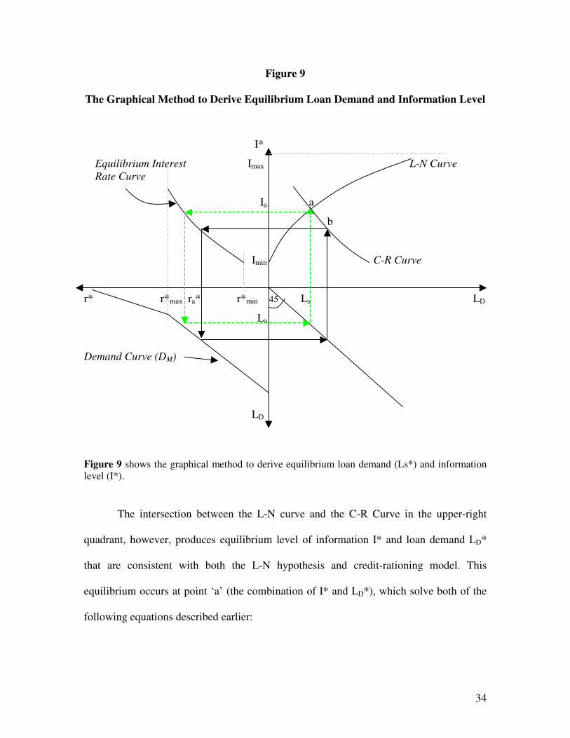
In the figure 9, the relationship 1, or the L-N Curve is shown in the upper-right
quadrant. The relationship 2, or the Equilibrium Interest Rate Curve is shown in the
upper-left quadrant. In the proposition 3 of the credit-rationing model, we show that the
equilibrium interest rate rises with the information levels. This positive relationship is
shown in this quadrant. The relationship 3, or the Demand Curve is depicted in the lower-
left quadrant. In the lower right has a 45-degree line that just reflects the value from the
negative y-axis to positive x-axis.
This graphical system helps us derive the credit-rationing curve (C-R Curve) in
the upper right quadrant. The C-R curve is the locus of all I and LD that result from the
credit-rationing model described in this paper. Two such points (point a and b) are
derived in the above graph: one shown by dotted line and the other by solid line. In both
these points, a given level of information (Ia, for point a) produces certain interest rate
(ra*) governed by Equilibrium Interest Rate Curve and the equilibrium interest rate (ra*)
produces a level loan demand (La) governed by the Demand Curve. The point a on the C-
R curve is composed of Ia and La. Connecting point a and point b, we can derive the C-R
Curve.
34
Figure 9
The Graphical Method to Derive Equilibrium Loan Demand and Information Level
I*
Equilibrium Interest Imax L-N Curve Rate Curve Ia a
b
Imin C-R Curve
r* r*max ra* r*min 45 La LD
La
Demand Curve (DM)
LD
Figure 9 shows the graphical method to derive equilibrium loan demand (Ls*) and information level (I*).
The intersection between the L-N curve and the C-R Curve in the upper-right
quadrant, however, produces equilibrium level of information I* and loan demand LD*
that are consistent with both the L-N hypothesis and credit-rationing model. This
equilibrium occurs at point ‘a’ (the combination of I* and LD*), which solve both of the
following equations described earlier:
35
(A) The L-N Process: I* = I (LD*)
(B) The Credit Rationing Model: LD* = L (r* (I*))
The loan demand La* in the upper-right produces Ia* level of information
according to the equation (A), or the L-N process. In the credit-rationing model, this
information affects equilibrium level of interest rate ra* in the upper-left quadrant.
According to the equation (B), the interest rate ra* is associated with La* level of loan
demand in the lower right-quadrant. Note, point b is not equilibrium because information
and loan demand combination in the C-R curve is not consistent with the L-N curve.
In the upper-right quadrant of the graph, the upper and lower limit of the
Equilibrium Interest Rate Curve is r*max and r*min respectively. The upper limit, or the
r*max that satisfies both the necessary and sufficient condition for r* [equation (17) and
(18)] is same as r*L, or the interest rate at which the low-risk borrowers drops out. This is
shown in the Appendix 2. The lower limit of the Equilibrium Interest Rate Curve, or the
r*min is associated with the maximum level of information or Imax. To see this, observe
how information affects interest rate in figure 7. In that figure, as information increases
equilibrium interest rate rises, but the minimum required interest rate for positive profit
falls. At the Imax, minimum required interest rate for positive profit riches to the
minimum11. In the lower-left quadrant, r*max is equal to rL and shows the maximum
interest rate threshold for pooling component. Beyond rL, we will be in the separating
component of the loan demand function where the definition of credit rationing does not
apply.
11 Note, r*min can be further bounded by the �min in the figure 4, where �min is the rate of return below which no commercial projects or mortgage will be funded. In the figure, we assumed that r*min defined by the Imax is greater than �min.
36
This graphical system clearly shows how loan demand affect the level of
information [the L-N process] and level of information affects equilibrium level of
interest rate and loan demand [credit-rationing model]. The S-W model shows the effect
of adverse selection on the credit rationing. This paper extends the S-W model by
incorporating the effect of information externalities.
The Existence and Uniqueness of the Equilibrium
The general equilibrium described in the previous subsection may not exist.
However, whenever the equilibrium exists it is unique. Note in the figure 9, the C-R
curve is bounded by the upper and lower limits of the Equilibrium Interest Rate Curve12.
Therefore, if the L-N curve rises very steeply from Imin and approaches to Imax without
ever crossing the bounded C-R curve, then the general equilibrium may not exist.
However, when the L-N curve and the C-R curve intersect, they must cross once.
Therefore, the equilibrium is unique. This single crossing is ensured by the monotonic
nature of the L-N and the C-R curve13.
Stability of the General Equilibrium
The equilibrium level of I* and LD* is stable and can be explained using a simple
numerical example. Lets assume minimum level of information available to all lenders is
IMIN=2 and IMAX=10. Suppose current information level I1=4 that generates equilibrium
12 Since r* is needs to exist to determine I and LD combination of the C-R curve, whenever r* does not exists or undefined the C-R curve is undefined as well. 13 Note the L-N curve is a monotonically increasing curve by assumption about the information generation process. The C-R will be monotonic whenever the Equilibrium Interest Rate Curve is monotonic. By equation (18), dr*/dI > 0 for all I. Therefore, the Equilibrium Interest Rate Curve and the C-R curve are both monotonic.
37
interest rate r1*= 6% at which loan demand LD=1000. Now if according to L-N process
this loan volume produces an information level I2=6 then I and LD are inconsistent and
we are out of equilibrium. At this stage, if the equilibrium is stable then disequilibrium
will create prerequisites to move toward the equilibrium. In the example, we have more
information than what is consistent with 1000 loan demand. So according to equation 21,
the lender will raise their interest rate, which will reduce the loan demand and level of
information generated. Now if this new level of information is consistent with increased
interest rate then we will be at the equilibrium else next round of change in the interest
rate will take place until equilibrium is achieved. In other words, if we are in
disequilibrium, interest rate response from the credit-rationing model makes the model
move toward equilibrium. Therefore, it is a stable equilibrium.
Comparative Static with the General Equilibrium
Analytical solution of the general equilibrium can be obtained by solving two
equations simultaneously. These equations are,
I* = I ( LD* ) and
LD* = LD ( r* ( I* ) )
Substituting the second equation into the first we get,
I* = I ( LD ( r* ( I* ) ) ) (22)
Equation (22) characterizes the equilibrium solution. This equation allows us to
see the comparative static of the parameters in the model on the equilibrium results.
Specifically, we look at the comparative static of four important policy parameters to see
the effects of these parameters on the equilibrium level of information generated (I*), the
38
interest offered (r*) and the loan volume demanded (LD*). The four policy parameters
are: the cost of fund rate (c), loss of rate of return associated with the high-risk borrowers
(�), the shift parameter measuring the total loan demand without affecting the
composition of low- and high-risk borrowers (�) and the parameter affecting the
borrower composition without changing the total loan demand (�). Detailed derivations
of the comparative results are shown in the appendix 3. Definition of key parameters and
summary of the comparative static on the general equilibrium results are shown in the
table 1 and table 2 respectively.
Table 1
Definition of Key Parameters in the Model
Symbol Definition
c Cost of fund rate.
� Parameter that increases the total loan demand without affecting composition of low- and high-risk borrower.
� Parameter that increases the share of high-risk borrowers without affecting the total loan demand.
� Cost associated with the high-risk borrowers.
� Rate of return.
r Interest rate.
I Level of information.
Ld(r) Loan demand function.
�i Proportion of low- and high-risk borrowers in the application pool. Here, i = L or H.
39
Table 2
Comparative Static
In the table, we see that a change in the cost of fund rate, or c has no effect on the
equilibrium levels. Note that the cost of fund rate negatively affects the pooled rate of
return function, or �L(r,c) - �(I).�H(r), which shifts the supply curve vertically without
affecting the equilibrium interest rate, or the r* [see figure 10].
Parameter Comparative Static Sign
D I* / d c 0
D r* / d c 0
c
D LD*/d c 0
D I* / d � >0
D r* / d � >0
�
D LD*/d � >0
D I* / d � >0
D r* / d � <0
�
D LD*/d � >0
D I* / d � >0
d r* / d � <0
�
d LD*/d � >0
40
Figure 10
The Effect of the Cost of Fund Rate (c) on the Equilibrium Interest Rate (r*)
�l(r) and
�.�h(r) �l(r)1 �l(r)2
�.�h(r)
�
c1 c2 r* rl r
- c1
- c2
�m(r)
Pooling Component Separating Component
r* rl r
Figure 10 in the upper panel, an increase in c reduces the �l(r). In the lower panel, market rate of return, or �m(r), which is the difference between �l(r) and �.�h(r), shifts down. Note, the interest rate at which the rate of return is maximized, r* remains unchanged.
41
The effect of the cost of fund rate on the equilibrium interest rate is shown in the
figure 10. Since the r* remains unchanged, according to the demand curve the
equilibrium loan demand (LD*) does not change and therefore, according to the L-N
curve the equilibrium level of information (I*) remains unchanged as well. In the figure,
the cost of fund rate increases from c1 to c2, which shifts the rate of return function for the
low-risk borrowers down from �l(r)1 to �l(r)2 in the upper panel. The change in c,
however, does not affect �.�h(r). Therefore, the pooled rate of return, or �l(r) - �.�h(r)
shifts down as shown by the dotted line in the lower panel. Note that c has no effect on
the credit rationing equilibrium r*. The interest rate at which the lenders’ rate of return is
maximized remains unchanged. Therefore, when cost of fund rises, rate of return falls,
less loanable funds the supplied to the mortgage market. However, the equilibrium
interest rate, loan demand and information remain unchanged. On the other hand, when
cost of fund rate falls, the rate of return rises. Since the loan supply function is the
monotonic function of rate of return, the loan supply increases as well. However, the
equilibrium interest rate, loan demand and information remain unchanged. Therefore, this
model suggests that lowering the cost of fund will increase the loan supply and will have
an effect in mitigating the credit rationing without affecting the loan demand or the
composition of the borrower types.
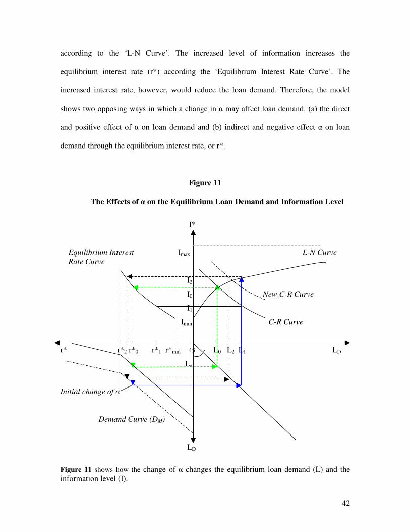
An increase in the parameter � increases in loan demand without changing the
proportion of low- and high-risk borrowers. When � increases, the loan demand curve
shifts up as shown by the dotted line in the lower left quadrant in the figure 11 increasing
the number of loans demanded at all interest rates. In the figure, initially the loan demand
goes up from L0 or L1. Because of increased loan demand, more information is generated
42
according to the ‘L-N Curve’. The increased level of information increases the
equilibrium interest rate (r*) according the ‘Equilibrium Interest Rate Curve’. The
increased interest rate, however, would reduce the loan demand. Therefore, the model
shows two opposing ways in which a change in � may affect loan demand: (a) the direct
and positive effect of � on loan demand and (b) indirect and negative effect � on loan
demand through the equilibrium interest rate, or r*.
Figure 11
The Effects of � on the Equilibrium Loan Demand and Information Level
I*
Equilibrium Interest Imax L-N Curve Rate Curve I2
I0 New C-R Curve
I1
Imin C-R Curve
r* r*2 r*0 r*1 r*min 45 L0 L2 L1 LD
La
Initial change of �
Demand Curve (DM)
LD
Figure 11 shows how the change of � changes the equilibrium loan demand (L) and the information level (I).
43
In the figure, the initial equilibrium is shown as the intersection between the C-R
curve and the L-N curve (point I0 and L0). Initially, as � rises loan demand increases from
L0 to L1 in the lower-left quadrant, This puts the system out of the general equilibrium.
Specifically, L1 number of loan produces the information level I2 through the L-N curve,
but according to the C-R curve I1 level of information is consistent with the L1 number of
loans. Since I1 is less than I2, the system is out of equilibrium.
To see the new equilibrium, note the change in � has no effect on the L-N curve.
However, the C-R curve shifts in response to the change in the loan demand and
equilibrium interest rate. Note, the C-R curve is drawn according to credit-rationing
model described by LD=LD (r*(I)), which is the locus of LD and I. Any given level of
information (I) produces an equilibrium interest rate (r*) according to ‘Equilibrium
Interest Rate Curve’ and the r* produces the loan demand (LD) according to the ‘Demand
Curve’. For example, combination (I0,L0) and (I1,L1) are two points on the initial C-R
curve. With an increase in �, the loan demand increases from L0 to L1 and the
information increases from I0 to I2. However, L1 and I2 and not consistent with the credit
rationing model or LD=LD (r*(I)). Specifically, L1 is consistent with I1 level of
information, where I1<I2. Therefore, the equilibrium interest rate will rise due to excess
information. This will reduce the loan demand from L1 to L2. To see the shift in C-R
curve, note that by the definition of C-R curve, I2 and L2 must be a point on the new C-R
curve shown by the dotted line. The new equilibrium takes place at the intersection of the
new C-R curve and the unchanged L-N curve.
It is possible to identify that the direct effect of � will dominate the indirect effect
through the equilibrium interest rate. Note that an increase in the loan volume generates
44
more information (according to the L-N Curve) and higher equilibrium interest rate
(according to the Equilibrium Credit Rationing Curve). The higher interest rate reduces
the loan demand, but the loan demand cannot be lower than the initial loan demand under
the assumption that the information is a positive monotonic function of loan volume
described by the L-N curve and equilibrium must occur on the L-N curve, which remains
unchanged with �. When loan volume increases, information increases unambiguously. If
the information increases interest rates such that loan volume falls, then this implies that
at the equilibrium, information may rise and loan volume may fall at the same time.
However, since equilibrium must occur on the monotonically positive L-N curve, the
rising information and falling loan volume cannot be sustained. In other word, loan
volume falls with information. However, the information can only increase if loan
volume rises. Therefore, the direct effect must dominate the indirect effect. The appendix
3 shows that the direct effect of loan demand dominates the indirect effect.
The dominance of the direct effect provides important intuition about the credit-
rationing situation in the market. Note, the direct effect of � increases the total loan
demand. This worsens the credit rationing in the market. However, according to the
indirect effect, � also increases the equilibrium interest rate (r*). This mitigates the credit
rationing at the cost of worse pool quality. In other words, as r* rises, loan demand falls,
therefore the credit rationing decreases. However, as r* rises, the share of the high-risk
borrowers rises relative to the low-risk borrowers, therefore the pool quality worsens.
Since the direct effect dominates and the net effect is the increase in the loan demand,
this implies that although the worse pool quality reduces the credit rationing, higher loan
demand increases the credit rationing more than the former reduction.
45
The parameter � increases the share of the high-risk borrowers in the pool without
affecting the total loan demand. The impact of � can be explained using the same
graphical system. Since � does not change loan demand directly, the demand curve
remains unaffected. However, the ‘Equilibrium Interest Rate Curve’ in the upper-right
quadrant shifts in response to �. This is shown analytically using the implicit function
theorem in the appendix 2. To see this intuitively, recall that the rate of return function is
�L(r,c) - �(I).�H(r). Since � increases �H(r), the rate of return falls with �. The falling rate
of return would induce lenders to improve the pool quality14 by lowering the equilibrium
interest rates (r*) at all levels of information. Therefore, the ‘Equilibrium Interest Rate
Curve’ shifts down. As the r* shifts down, the loan demand rises according to the
demand curve and level of information rises according to the L-N curve. The increased
information, however, increases the equilibrium interest rate (r*) along to new
‘Equilibrium Interest Rate Curve’. Therefore, the parameter � will affect the equilibrium
interest rate (r*) in two opposing ways: (a) direct effect when ‘Equilibrium Interest Rate
Curve’ shifts down and r* falls and (b) indirect effect when r* rises as the loan volume
and information rises in response to the direct effect.
It is possible to show that the direct effect of the parameter � will dominate the
indirect effect, and the overall effect will be the reduction of the equilibrium interest rate
(r*). When � rises, the ‘Equilibrium Interest Rate Curve’ shifts down and r* falls at all
levels of information. Consequently, the loan demand rises. However, if indirect effects
dominates, the r* rises and consequently loan demand and information level falls. As
mentioned before, increased loan demand and decreased level of information cannot
14 Improvement of pool quality means making more loans to the low-risk borrowers.
46
occur at the same time in the equilibrium. This is because according to the L-N
hypothesis information is a monotonically increasing function of the loan demand.
Therefore, direct effect must dominate the indirect effect of �.
The dominance of the direct effect again would provide important intuition about
the credit-rationing situation in the market. Since the direct effect dominates and the net
effect is the reduction in the equilibrium interest rate (r*), this implies that an increase in
�, or the share of the high-risk borrowers, is associated with the lower equilibrium
interest rate, higher loan demand and therefore, increased credit rationing. However,
since lower equilibrium interest rate induces low-risk borrowers to apply, the increased
credit rationing is also associated with improved pool quality. Conversely, this model
suggests that by lowering �, the equilibrium interest rate rises, loan demand falls and
therefore, credit rationing reduces. However, this improvement in credit rationing occurs
at the cost of worsening pool quality.
The loss associated with the high risk borrowers or parameter � has almost an
identical effect as � on the equilibrium loan demand and information level. Similar to �,
when the parameter � rises, the rate of return function or �L(r,c) - �.�H(r) falls, and
lenders respond to this change by lowering the equilibrium r* at all information levels in
order to improve the pool quality. Therefore, the parameter � and � will same effects.
Conclusion and Possible Extensions
This paper combines the S-W type credit-rationing model with the L-N type
information externalities. The S-W model shows how credit rationing emerges in the
presence of adverse selection. This paper explicitly incorporates the information
47
externalities produced by neighborhood specific market activities into the credit-rationing
model and shows one of the sufficient conditions in which credit rationing is reduced as
the level of information rises. This is in line with theoretical papers that show other
sufficient conditions for the disappearance of credit rationing through mitigation of
adverse selection or separation of risk types [see Bester 1985, Besanko and Thakor 1987,
Calem and Stutzer 1995 and Ben Shahar and Feldman 2001].
In addition, the previous studies have not considered the equilibrium properties of a
credit-rationing model in the presence of information externalities. Information increases
lenders’ ability to minimize loss and increases their willingness to supply credit affecting
the level credit rationing at all interest rates. Increased supply of credit, however,
generates more information. This suggests a general equilibrium set up where equilibrium
credit rationing and information level are jointly determined. The S-W type credit-
rationing models cannot provide the insights obtained from a model that recognizes the
existence of information externalities. For example, the partial equilibrium model shows
that the equilibrium interest rate increases and the credit rationing decreases with
information, but does not consider the feed back effect of the increased interest rate. By
incorporating the L-N type information externalities, we can show how the increased
interest rate, and consequently the reduced loan volume in turn determine the level of
information generated at the equilibrium. Similarly, the L-N hypothesis of information
externalities is also incomplete in the sense that it shows how loan volume or market
activities generate information, which in turn facilitates further production of loans.
However, it does not consider that the effect of increased information on the equilibrium
interest rate offered. Specifically, we find that increased information through market
48
activities increases the equilibrium interest rate and reduces the loan volume. This paper,
therefore, suggest that the loan volume in the L-N type information externalities models
may be mitigated by the increased interest rate associated with the externalities.
Consequently, empirical research may find reduced effect of the L-N type information
externalities.
This paper suggests several policy implications relating to the mortgage credit
market. The paper shows that information dissemination may reduce credit rationing but
at the cost of increasing interest rates. Specifically, increased information reduces the loss
of rate of return associated with the lending to high-risk borrowers. This allows lenders to
increase the interest rate. However, since low-risk borrower stop seeking credit at certain
interest rate, increase in the interest rate changes the composition of borrowers served by
the lending institutions. Therefore, this paper allows policy makers to carefully consider
the benefits of reduced credit rationing with the potential cost of increase in the interest
rates, and its adverse effects on the composition of borrowers who apply for loans.
In addition, the comparative static analysis of this paper shows the effect of
several policy parameters such as, cost of fund rate (c), total loan demand keeping
composition of low- and high-risk borrowers in the market unaffected (�), composition of
low- and high-risk borrowers keeping total loan demand unaffected (�) and loss of return
associated with the high-risk borrowers (�). These results can be important in evaluating
policy relating to credit markets. For example, the paper shows that reduction of the cost
of fund rate (c) has no effect on the equilibrium interest rate offered by the lender, but can
reduce the credit rationing without affecting the total loan demand or the borrower
composition. However, the effect of � is not straightforward. The direct effect of �
49
increases the loan demand and therefore, increases the credit rationing. The indirect effect
of � increases the equilibrium interest rate and therefore, reduces credit rationing at the
cost of worse pool quality. Since the direct effect dominates and the net effect is the
increase in the loan demand, this implies that � increases the credit rationing in the
markets. On the other hand, the direct effect of � and � decreases the equilibrium interest
rate (r*). Therefore, the loan demand rises, pool quality improves and the credit rationing
increases. The indirect effect of � and �, however, increases the equilibrium interest rate
due to increases market activities and information level. Therefore, the loan demand falls,
pool quality worsens and the credit rationing decreases. Since the direct effect dominates
and the net effect is the decrease in the interest rate, this implies that by increasing � or
�15, the credit can be worsens, but pool quality improves. Conversely, this model suggests
that by lowering � or �, the credit rationing can be improved at the cost of worsening pool
quality.
This paper can be a simple building block to analyze credit market characterized
by both adverse selection and information externalities. The paper might be helpful in
modeling the effect of different institutional structures of mortgage lending institutions
including monopolistic lender. For example, the framework described in the paper may
be used to understand the credit rationing and level of information generated when the
lenders are monopolistic. A monopolistic lender will have higher information advantage,
which might induce higher loan volume. However, it will have lower loan production due
to monopoly nature. Additionally, this paper can be useful in comparing efficiency in
terms of loan supply, information generation and credit rationing associated with
15 Increasing � means increasing the share of the high-risk borrowers and increasing � means increasing the loss associated with high-risk borrowers.
50
different alternative schemes proposed in the literature that attempts to increase lending
to low- and moderate-income borrowers including non-profit lending and the CRA
permit [Richardson 2002].
51
References:
R. B. Avery, P.E. Beeson, and M.S. Sniderman, Neighborhood information and home
mortgage lending, Journal of Urban Economics 45 (1999) 287-310.
D. Ben-Shahar and D. Feldman, Signaling-screening equilibrium in the mortgage market,
The Journal of Real Estate Finance and Economics 26 (2003) 157-178.
D. Besanko and A.V. Thakor, Collateral and Rationing: Sorting Equilibria in Monopolist
and Competitive Credit markets, International Economic Review, 28 (1987) 671-689.
H. Bester, Screening vs. Rationing in Credit Markets with Imperfect Information, The
American Economic Review 75 (1985) 850-855.
J. K. Brueckner, Mortgage Default with Asymmetric Information, 20 (2000) 251-274.
P. S. Calem, Mortgage credit availability in low- and moderate-income minority
neighborhoods: are information externalities critical? Journal of Real Estate Finance and
Economics 13 (1996) 71-89.
P.S. Calem and M. J. Stutzer, The Simple Analytics of Observed Discrimination in Credit
Markets, Journal of Financial Intermediation 4 (1995) 189-212.
A. C. Cutts and R. Van Order, On the Economics of Subprime Lending, Freddie Mac
Working Paper (2004) #04-01.
D. M. Harrison, Importance of Lender Heterogeneity in Mortgage Lending, Journal of
Urban Economics 49 (2001) 285-309.
52
A.R. Hossain and S.L. Ross, A Direct Test of the Lang and Nakamura Hypothesis of
Information Externalities over Space, Eonometric Society 2004 North American Summer
Meetings # 398 (2004).
W. W. Lang and L. I. Nakamura, A Model of Redlining, Journal of Urban Economics 33
(1993) 223-234.
D. C. Ling and S. M. Wachter, Information externalities and home mortgage
underwriting, Journal of Urban Economics 44 (1998) 317-332.
C.A. Richardson, The Community Reinvestment Act and the Economics of Regulatory
Policy. Fordham Urban Law Journal, 4 (2002).
M. Rothschild and J.E. Stiglitz, Equilibrium in Competitive Insurance Markets: An Essay
in the Economics of Imperfect Information, Quarterly Journal of Economics 80 (1976)
629-649.
J.E. Stiglitz and A. Weiss, Credit Rationing in Markets with Imperfect Information,
American Economic Review 71 (1981) 393-410.
53
APPENDICES Appendix.1
Cases of Credit Rationing
Case 1: rm > rl and rationing is more profitable than subprime (only to high risk) lending. Equilibrium interest rate is r* and credit rationing occurs. L
LS
LD
r* rl rm rh r
Case 2: rm > rl and rationing is less profitable than subprime (only to high risk) lending. Equilibrium interest rate is rm. Loans are offered only to high-risk borrowers, therefore no credit-rationing. Note the sufficient condition �m(r*) > �m(rm) is violated. L
LS
LD
r* rl rm rh r
54
Case 3: r* <rm < rl or rationing is more profitable than prime (pooled) lending. Equilibrium interest rate is r*. Credit rationing occurs.
L
LS
LD
r* rm rl rh r
Case 4 rm < r* < rl or rationing is less profitable than prime (pooled) lending. Equilibrium interest rate is rm and credit rationing disappears. Note the necessary condition ��pool(r*) = 0 such that r*<rm is violated.
L
rm r* rl rh r
55
Appendix 2 In this appendix, we show the following proposition. Proposition: The upper limit of the equilibrium credit rationing interest rate, or the r*max that satisfies both the necessary and sufficient condition for equilibrium credit rationing interest rate, or the r* is the interest rate at which the low-risk borrowers drops out, or the rL. To show this, we will use the appendix 2 that describes all possible cases of credit rationing. Recall the necessary condition for the credit rationing equilibrium in the equation 17 is, ��pool(r*) = 0 such that r* < rm. This implies that equilibrium credit rationing must occur before the market clearing interest rate. This eliminates case 4 described in the appendix 1. Among the remaining cases, the case 2 is violates the sufficient condition �m(r*) > �m(rm). In this case, lenders prefer to supply all credits to high-risk borrowers, perhaps in the subprime market. Therefore, this paper focuses on the credit rationing described by case 1 and 3. In the case 3, r* is bound by rm. This is true because if r*max < rm, it will be similar to the case 4 and the necessary condition for the equilibrium will be violated. Therefore, Lim (r*max) = rm. Note, however, that in the case 3, rm is less than rL. Therefore, rL is still the upper limit of rm. In other words, the rm can rise and move left toward rL. However, If rm>rL, the case 3 becomes the case 1 in the appendix 1. Therefore, this proposition reduces to showing that in the case 1 maximum value of r* is rL. Recall that the necessary condition for r* is
��pool(r*) = 0 such that r* < rm
This implies that,
�L�(r) = � .�H� (r) However, when r > rL or at the separating component of demand, �L�(r) > 0 and � .�H� (r) = 0. Therefore, rate of return rises with interest rate above rL indefinitely. Therefore, r*max is not bounded. At the r=rL, � .�H� (r) is undefined. When r<rL, both the �L�(r) > 0 and � .�H� (r)>0. The necessary condition can be satisfied at r � [0, rL). Therefore, the upper limit of r*max is rL. The sufficient condition is also satisfied since �H�� (r)>0. The r*max that occurs at the limit can be shown in the following figure.
56
The Maximum Equilibrium Interest Rate r*max
�l(r) and �.�h(r)
�l(r)
�
�.�h(r)
c r* rL r
- c
�m(r)
Pooling Component Separating Component
�h = �l(r)- �
�pool = �l(r) - �.�h(r)
lim(r*max) = rL r
57
lL
l
hH
Appendix. 3Comparative Statics
Recall the demand function:
[d(r)- ] when r < rLow Risk: D =
0 when r r
[d(r)+ ] when r < rHigh Risk: D =
0 when r
α θ
α θ
� �� �≥� �
hr
Here, represents a parameter that changes total loan volume without affecting the relative share of loan
demand by two types of borrowers. represents a parameter that changes the share of l
α
θ
� �� �≥� �
oan demand by two types of borrowers without affecting the total loan demand.d(r) is a general negatively sloped function. Therefore, d '(r) < 0
Vertical summation of demand functions of both types giv
l
M h
h
es market demand function as follows,
2 d(r) when r < r
Market Demand: D [d(r)+ ] when rl r < r
0 when r r
From the demand function we calculate the shares of l
αα θ� �� �= ≤� �� �≥� �
ll
l
lh
l
oan demand among two risk types:
d(r)- when r < r
2d(r)low risk: =0 when r r
d(r)+ when r < r
2d(r)High risk: = 1 when r r
The equilibr
θδ
θδ
� �� �� �� �≥� �
� �� �� �� �≥� �
h
ium credit rationing interest rate, r* is defined by the F.O.C. At r*, '(r*,c) - ( ). '( *, ) 0
From the F.O.C., r*( (I),c, ) is a function of parameter I,c,
Implicit Function Theorem provides,- '( ). '( *, )*
1. 0
( '( *, ))- ( ).*
2.
Recall, '( , )
h
I rdrdI SOC
d rI
dr dd SOC
r
β θ θ
β δ θ
δ θβ
θθ
δ θ
= − >
= −
= h2 2
( '( *, ))- 2.d'(r). - 2.d'(r) therefore, = > 0
4[d(r)] 4[d(r)]( '( *, ))
- ( ).* Therefore, 0
( '(r*,c))*
3.
Recall, '(r*,c)=1 ther
h
d rd
d rI
dr dd SOC
ddr dcdc SOC
δ θθθ
δ θβ
θθ
ρ
ρ
= − <
= −
h
( '(r*,c))efore, 0
( '(r*,c))*
Threfore, 0
- '( *, )*4. 0
General Equilibrium Solution
ddc
ddr dcdc SOC
rdrd SOC
ρ
ρ
δ θβ
=
= − =
= − <
D
D D
D
1. L-N hypothesis: I*=I(L* )
2. Credit Rationing: L* = L (r*(I*))
Substituting 2 into 1: I*=I(L (r*(I*)))
Inserting loan demand in the pooling equilibrium: I* = I(2.�.d(r*(I*)))
59
�
[ ]
��
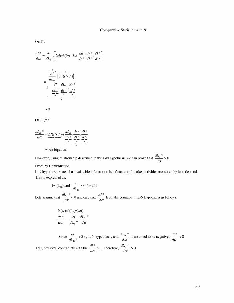
Comparative Statistics with
On I*:
* * *. 2 (r*(I*)+2 . . .* *
. 2 (r*(I*)
1 . .*
D
D
D
D
dI dI dd dr dId
d dL dr dI d
dId
dLdLdI
dL dr
α
αα α
++
−+
� = ��
=−
�����
�
**
> 0
drdI
+
+��������
� � �
D
+
On L * :
* * *2 (r*(I*) + . .
* *
= Ambiguous.*
However, using relationship described in the L-N hypothesis we can prove that 0
Proof by Contradiction:L-N hyp
D D
D
dL dL dr dId
d dr dI d
dLd
α α
α
− + +
−
=
>
����
������
DD
othesis states that avaialable information is a function of market activities measured by loan demand. This is expressed as,
I=I(L ) and 0 for all IL
*Lets assume that 0 anD
dId
dLdα
>
<
D
D
D
*d calculate from the equation in L-N hypothesis as follows.
I*( )=I(L *( ))
** .
L *
Since >0 by L-N hypoL *
D
dId
dLdI dId d d
dId
α
α α
α α=
* *thesis, and is assumed to be negative, < 0
**This, however, contradicts with the 0. Therefore, > 0
D
D
dL dId d
dLdId d
α α
α α>
60
On r*:Since r*(I,c, ) is a function of I, c and , does not shifts the equilibrium interest rate curve. However, affects r* through information as follows:
r*(I( ),c, ) r*(I( ),c, ).
d d dd dI
θ θ αα
α θ α θα
+
=������
(I( ),c, )0
Comparative Statistics with
On r*:Using Implicit Function Theorem, we have shown previously that,
dr* < 0
d
O
dα θ
α
θ
θ
+
>����
� � �
�� �
D
D
D
D D
n I*:Recall I* = I(2.�.d(r*(I*,c, )))
I* d * * * 2 . .* *
This simplifies to,
dI *. .
dL *dI* > 0
dI *d1 . .
dL *
On L *:
Recall L * = L (r*(I*,c, ))
d
D
D
D
d dI d dr dI drd dL dr dI d d
dL drdr d
dL drdr dI
θ
αθ θ θ
θθ
θ
−+ −
− ++
� � = + � �� �
=−
�� � �
D D
D
D
dr* dI dr*L * dL . dI d dd dr
= AmbiguousdL *dI* dI
However, since 0 and 0 by L-N hypothesis, we can show that 0d dL d
θ θθ
θ θ
+ + −−
� + �= ��
> > >
61
Comparative Statistics with
On r*:Using Implicit Function Theorem, we have shown previously that,
dr* < 0
d
On I*:Recall I* =
β
β
�
� �
��
-+
D
D D
D D
I(2.�.d(r*( (I*),c, )))
d *I* 2 . . > 0*
On L *:
Recall L * = L (r*( (I*),c, ))
dL * dL dr* . > 0
d dr d
D
d drd dIdr dd dL
β θ
αββ
β θ
β β
−
− −
� �= ��
=
Comparative Statistics with c
On r*:Using Implicit Function Theorem, we have shown previously that,