Mon. Not. R. Astron. Soc. 000, 000–000 (0000) Printed 9 March 2015 (MN LATEX style file v2.2)

A Study of Multi-frequency Polarization Pulse Profiles ofMillisecond Pulsars

S. Dai1,2, G. Hobbs2, R. N. Manchester2, M. Kerr2, R. M. Shannon2, W. van Straten3,A. Mata4, M. Bailes3, N. D. R. Bhat5, S. Burke-Spolaor6, W. A. Coles7, S. Johnston2,M. J. Keith8, Y. Levin9, S. Os lowski10,11, D. Reardon9,2, V. Ravi12, J. M. Sarkissian13,C. Tiburzi14,15,2, L. Toomey2, H. G. Wang16,2, J.-B. Wang17, L. Wen18, R. X. Xu1,19,W. M. Yan17, X.-J. Zhu181School of Physics and State Key Laboratory of Nuclear Physics and Technology, Peking University, Beijing 100871, China2CSIRO Astronomy and Space Science, Australia Telescope National Facility, Box 76 Epping NSW 1710, Australia3Centre for Astrophysics and Supercomputing, Swinburne University of Technology, PO Box 218, Hawthorn, VIC 3122, Australia4Center for Advanced Radio Astronomy, University of Texas, Rio Grande Valley, Brownsville, TX 78520, USA5International Centre for Radio Astronomy Research, Curtin University, Bentley, WA 6102, Australia6Department of Astronomy, California Institute of Technology, Pasadena, CA 91125, USA7Department of Electrical and Computer Engineering, University of California, San Diego, La Jolla, CA 92093, USA8Jodrell Bank Centre for Astrophysics, University of Manchester, M13 9PL, UK9School of Physics and Astronomy, Monash University, Victoria 3800, Australia10Max-Planck-Institut fur Radioastronomie, Auf dem Hugel 69, D-53121 Bonn, Germany11Department of Physics, Universitat Bielefeld Universitatsstr. 25 D-33615 Bielefeld, Germany12School of Physics, University of Melbourne, Parkville, VIC 3010, Australia13CSIRO Astronomy and Space Science, Parkes Observatory, Box 276, Parkes NSW 2870, Australia14INAFOsservatorio Astronomico di Cagliari, Via della Scienza, I-09047 Selargius (CA), Italy15Dipartimento di Fisica, Universita di Cagliari, Cittadella Universitaria, I-09042 Monserrato (CA), Italy16School of Physics and Electronic Engineering, Guangzhou University, 510006 Guangzhou, China17Xinjiang Astronomical Observatory, Chinese Academy of Sciences, 150 Science 1-Street, Urumqi, Xinjiang 830011, China18School of Physics, University of Western Australia, Crawley, WA 6009, Australia19Kavli Institute for Astronomy and Astrophysics, Peking University, Beijing 100871, China

9 March 2015

ABSTRACT

We present high signal-to-noise ratio, multi-frequency polarization pulse profilesfor 24 millisecond pulsars that are being observed as part of the Parkes Pulsar TimingArray (PPTA) project. The pulsars are observed in three bands, centred close to 730,1400 and 3100 MHz, using a dual-band 10 cm/50 cm receiver and the central beamof the 20 cm multibeam receiver. Observations spanning approximately six years havebeen carefully calibrated and summed to produce high S/N profiles. This allows usto study the individual profile components and in particular how they evolve withfrequency. We also identify previously undetected profile features. For many pulsarswe show that pulsed emission extends across almost the entire pulse profile. Thepulse component widths and component separations follow a complex evolution withfrequency; in some cases these parameters increase and in other cases they decreasewith increasing frequency. The evolution with frequency of the polarization propertiesof the profile is also non-trivial. We provide evidence that the pre- and post-cursorsgenerally have higher fractional linear polarization than the main pulse. We haveobtained the spectral index and rotation measure for each pulsar by fitting acrossall three observing bands. For the majority of pulsars, the spectra follow a singlepower-law and the position angles follow a λ2 relation, as expected. However, cleardeviations are seen for some pulsars. We also present phase-resolved measurementsof the spectral index, fractional linear polarization and rotation measure. All theseproperties are shown to vary systematically over the pulse profile.

Key words: polarization − pulsars : general − radiation mechanisms : nonthermal− radio continuum

c© 0000 RAS

arX

iv:1

503.

0184

1v1

[as

tro-

ph.G

A]

6 M

ar 2

015

2 S. Dai et al.

1 INTRODUCTION

Millisecond pulsars (MSPs) are a special subgroup of ra-dio pulsars. Compared with ‘normal’ pulsars, they haveshorter spin periods and much smaller spin-down rates, andtherefore have larger characteristic ages and weaker implieddipole magnetic fields. The short spin periods and highlystable average pulse shapes of MSPs make them powerfultools to investigate a large variety of astrophysical phenom-ena. In particular, much recent work has been devoted toa search for a gravitational-wave background using obser-vations of a large sample of MSPs in a “Pulsar Timing Ar-ray” (e.g., Foster & Backer 1990). The Parkes Pulsar TimingArray (PPTA) project (Manchester et al. 2013) regularly ob-serves 24 MSPs. The PPTA search for gravitational waveshas been described in other papers including Shannon et al.(2013), Zhu et al. (2014) and Wang et al. (2015).

We have not yet detected gravitational waves. In orderto do so we will need to observe a larger set of pulsars, in-crease the span of the observations and/or to increase thetiming precision achieved for each observation (e.g., Cordes& Shannon 2012). Determining whether it is possible to im-prove the timing precision and, if so, by how much relieson our understanding of the stability of pulse profiles (e.g.,Shannon et al. 2014) and also on the profile frequency evolu-tion and polarization properties. For our work we study thelarge number of well calibrated, high signal-to-noise ratio(S/N) multi-frequency polarization pulse profiles that havebeen obtained as part of the PPTA project.

An earlier analysis of the 20 cm pulse profiles from thePPTA sample was published by Yan et al. (2011a). This ear-lier work is extended in this paper as: (1) we include fournew pulsars that have recently been added to the PPTAsample; (2) we utilise more modern pulsar backend instru-mentation than was available to Yan et al. (2011a); (3) weuse longer data sets enabling higher S/N profiles; and (4)we provide polarization pulse profiles in three independentbands (at 10, 20 and 50 cm). We note that, even though wehave mainly the same sample of pulsars as was described byYan et al. (2011a), our data sets are independent (i.e., nodata is in common between this and the earlier publication).

It has been shown that, compared with normal pulsars,the pulse profiles of MSPs usually cover a much larger frac-tion of the pulse period and, for measurements with the sameS/N, often exhibit a larger number of components (Yan et al.2011a). However, the spectra of MSPs and normal pulsarsare similar (Toscano et al. 1998; Kramer et al. 1998, 1999a).Both MSPs and normal pulsars often have a high degree oflinear polarization and orthogonal-mode position angle (PA)jumps (see e.g., Thorsett & Stinebring 1990; Navarro et al.1997; Stairs et al. 1999; Manchester & Han 2004; Ord et al.2004). For MSPs the PAs often vary significantly with pulsephase and, in most cases, they do not fit the ‘rotating vectormodel’ (RVM, Radhakrishnan & Cooke 1969).

Various models exist to explain complex pulse profiles.Multiple emission cones have been proposed and discussedby several authors (Rankin 1983; Kramer 1994; Gupta &Gangadhara 2003). In another model the emission beamcontains randomly distributed emission patches (Lyne &Manchester 1988; Manchester 1995; Han & Manchester2001). It has also been suggested that the emission fromat least some young pulsars arises from the outermost open

field lines at relatively high altitudes (Johnston & Weisberg2006). Similarly, Karastergiou & Johnston (2007) proposedthat radio emission is confined to a region close to the lastopen field lines and arises from a wide range of altitudesabove the surface of the star at a particular frequency. Basedon investigations of the radio and gamma-ray beaming prop-erties of both normal pulsars and MSPs, Manchester (2005)and Ravi et al. (2010) proposed that the radio emission ofyoung and MSPs originates in wide beams from regions highin the pulsar magnetosphere (up to or even beyond the null-charge surface) and that features in the radio profile repre-sent caustics in the emission beam pattern.

To date, no single model can describe the observations.This paper is an observationally-based publication that wehope will shed new light on the MSP emission mechanism.We present the new profiles in three widely separated ob-serving bands and describe how they were created. We deter-mine various observationally-derived properties of the pro-files (such as spectral indices, polarization fractions, etc.)and study how such parameters vary between pulsars andwith frequency. Using these high S/N profiles, we also carryout phase-resolved studies of the spectral index (e.g., Lyne& Manchester 1988; Kramer et al. 1994; Manchester & Han2004; Chen et al. 2007), linear polarization fraction, androtation measures (RMs) (e.g., Ramachandran et al. 2004;Han et al. 2006; Noutsos et al. 2009). The data describedhere will be used in a subsequent paper to study the sta-bility of the pulse profiles as a function of time, which isrelevant for high-precision pulsar timing experiments. In afurther paper, we will apply new methods (e.g., Pennucciet al. 2014; Liu et al. 2014) to improve our timing preci-sion using frequency-dependent pulse templates. Our datasets are publically available, enabling anyone to compare theactual observations with their models of the pulse profiles.

Details of the observation, data processing, and dataaccess are given in Section 2. In Section 3, we present themulti-frequency polarization pulse profiles. In Section 4, thepulse widths, flux densities and spectral indices, polariza-tion parameters and rotational measures are discussed. Asummary of our results and conclusions are given in Section5.

2 OBSERVATIONS AND ANALYSIS

2.1 Observations

We selected observations from the PPTA project of 24MSPs. The pulsars are observed regularly, with an approxi-mate observing cadence of three weeks, in three bands cen-tred close to 730 MHz (50 cm), 1400 MHz (20 cm) and 3100MHz (10 cm), using a dual-band 10 cm/50 cm receiver andthe central beam of the 20 cm multibeam receiver. The ob-serving bandwidth was 64, 256 and 1024 MHz respectivelyfor the 50 cm, 20 cm and 10 cm bands. We used both dig-ital polyphase filterbank spectrometers (PDFB4 at 10 cmand PDFB3 at 20 cm) and a coherent dedispersion machine(CASPSR at 50 cm). In Table 1, we summarize the observa-tional parameters for the 24 PPTA MSPs. For each band, wegive the number of frequency channels across the band, thenumber of bins across the pulse period, the total number ofobservations and the total integration time. In Table 2, we

c© 0000 RAS, MNRAS 000, 000–000

A Study of Multi-frequency Polarization Pulse Profiles of Millisecond Pulsars 3

give the basic pulsar parameters from the ATNF Pulsar Cat-alogue (Manchester et al. 2005). For each observing band,we also give the dispersion smearing and the pulse broad-ening time caused by scattering (in units of profile bins).The dispersion smearing across each frequency channel iscalculated according to

∆tDM ≈ 8.30× 106 DM ∆ν ν−3 ms, (1)

where ∆ν is the channel width in MHz, ν is the band centralfrequency in MHz, and DM is the dispersion measure in unitsof cm−3 pc. The pulse broadening time caused by scatteringis estimated according to

τd =1

2πν0, (2)

where ν0 is the scintillation bandwidth. We calculate thebroadening time in the 20 cm band using scintillation band-widths measured by Keith et al. (2013), and then scale itto the 10 cm and 50 cm bands according to τd ∝ ν−4. ForMSPs not in the sample of Keith et al. (2013), we mea-sure the scintillation bandwidths using the autocorrelationfunction (ACF) of the dynamic spectrum (e.g., Wang et al.2005). We note that in Table 2, we only list τd values thatare > 0.0001 bin and set others as zero.

To calibrate the gain and phase of the receiver system,a linearly polarized broad-band and pulsed calibration sig-nal is injected into the two orthogonal channels through acalibration probe at 45◦ to the signal probes. The pulsedcalibration signal was recorded for 2 ∼ 3 min prior to eachpulsar observation. Signal amplitudes were placed on a fluxdensity scale using observations of Hydra A, assuming a fluxdensity of 43.1 Jy at 1400 MHz and a spectral index of −0.91over the PPTA frequency range. All data were recorded us-ing the PSRFITS data format (Hotan et al. 2004) with 1-minsubintegrations and the full spectral resolution (for furtherdetails see Manchester et al. 2013, and references therein).

2.2 Analysis

The data were processed using the PSRCHIVE softwarepackage (Hotan et al. 2004). We removed 5 per cent ofthe bandpass at each edge and excised data affected bynarrow band and impulsive radio-frequency interference foreach subintegration. The polarization was then calibratedby correcting for differential gain and phase between thereceptors using the associated calibration files. For 20 cmobservations with the multibeam receiver, we corrected forcross coupling between the feeds through a model derivedfrom observations of PSR J0437−4715 that covered a widerange of parallactic angles (van Straten 2004).

The Stokes parameters are in accordance with the astro-nomical conventions described by van Straten et al. (2010).Stokes V is defined as ILH − IRH, using the IEEE definitionfor sense of circular polarization. The baseline region was de-termined with the Stokes I profile. The baseline duty cycleused for each MSP are presented in Table A1. Baselines forthe Stokes I, Q, U and V profiles were set to zero mean. Thelinear polarization L was calculated as L = (Q2 + U2)1/2,and the noise bias in L was corrected according to Equation11 in Everett & Weisberg (2001). The similar bias in |V | wascorrected as described in Yan et al. (2011a). The position an-gles (PAs) of the linear polarization refer to the band central

frequency and were calculated as ψ = 0.5 tan−1(U/Q) whenthe linear polarization exceeds four times of the baseline rootmean square (rms) noise. They are absolute and measuredfrom celestial north towards east, i.e. counterclockwise onthe sky. Errors on the PA values were estimated accordingto Equation 12 in Everett & Weisberg (2001).

In order to add the data in time to form a final meanprofile, pulse times of arrival were obtained for each ob-servation using an analytic template based on an existinghigh S/N pulse profile. The TEMPO2 pulsar timing softwarepackage (Hobbs et al. 2006) was then used to fit pulsar spin,astrometric, and binary parameters, and also to fit harmonicwaves as necessary to give white timing residuals for eachpulsar. Finally, the separate observations were summed us-ing this timing model to determine relative phases and formthe final Stokes-parameter profiles.

To give the best possible S/N in the polarization pulseprofiles, the individual observation profiles were weighted bytheir (S/N)2 when forming the average profile. As many ofthe pulsars scintillate strongly, this weighting implies that,for a few pulsars, the average profiles are dominated by afew individual observations with a high S/N. As discussedin Section 4 this can affect measurements of the spectral in-dex, fractional polarizations, and RMs. Also, if the pulseprofile varies with flux density (for instance, as seen forPSR J0437−4715 by Os lowski et al. 2014) then this weightedprofile will be biased towards the profile shape at high fluxdensity. We therefore have also produced average profilesusing only the observation time for weighting.

Since the PA of the linear polarization suffers Faradayrotation in the interstellar medium and in the Earth’s iono-sphere, this Faraday rotation must be removed to form themean polarization profiles. According to Yan et al. (2011b),the interstellar RMs of PPTA MSPs are stable, and for ourinitial analysis we used the best-available interstellar RMvalues for our sample (Keith et al. 2011; Yan et al. 2011a;Keith et al. 2012; Burgay et al. 2013). To account for thecontribution of the Earth’s ionosphere, we used the Interna-tional Reference Ionosphere (IRI) model 1.

For each MSP, we aligned the average pulse profile inthe 10 and 50 cm bands with respect to that in the 20 cmband. The technique we used is described in detail in Taylor(1992), which was originally developed for the measurementof pulse arrival times. We derived the phase shift betweenprofiles and the profile in the 20 cm band in the frequency do-main, rotated the profiles and then transformed them backto the time domain. With these aligned three-band profiles,we calculated the phase-resolved spectral indices, fractionallinear polarizations and RMs for each MSP. The spectralindex was fitted using a power-law of the form S = S0ν

α

and the fractional linear polarization was defined as 〈L〉/S,where S = 〈I〉 is the total intensity and L is the linear po-larization. The RM was obtained by fitting the PA acrossbands according to ψ = RM λ2, where λ = c/ν is the ra-dio wavelength corresponding to radio frequency ν. As manyof the MSP profiles have multiple components which varysignificantly with frequency, it is difficult to determine anabsolute profile alignment. Our cross-correlation method is

1 See http://iri.gsfc.nasa.gov for a general description of the

IRI.

c© 0000 RAS, MNRAS 000, 000–000

4 S. Dai et al.

Table 1. Observational parameters for the 24 PPTA MSPs.

PSR No. of channels No. of phase bins No. of observation epochs Integration time

(h)50 cm 20 cm 10 cm 50 cm 20 cm 10 cm 50 cm 20 cm 10 cm 50 cm 20 cm 10 cm

J0437−4715 256 1024 1024 1024 1024 2048 177 669 281 142.9 502.2 248.8

J0613−0200 256 1024 1024 1024 512 512 64 160 111 66.0 159.3 113.9J0711−6830 256 1024 1024 1024 1024 1024 72 161 102 65.9 161.1 102.2

J1017−7156 256 2048 2048 1024 256 512 85 135 73 86.5 130.4 76.3

J1022+1001 256 1024 1024 1024 2048 2048 65 148 117 58.4 138.3 110.5

J1024−0719 256 1024 1024 1024 1024 1024 34 112 59 36.1 111.0 61.5

J1045−4509 256 2048 1024 1024 512 1024 63 137 103 42.7 138.9 104.5J1446−4701 256 512 1024 1024 512 1024 19 50 9 15.2 39.4 8.8

J1545−4550 256 1024 1024 1024 512 1024 15 21 15 13.2 20.6 12.2J1600−3053 256 1024 1024 1024 512 512 53 139 106 56.6 129.9 108.0

J1603−7202 256 2048 1024 1024 1024 1024 52 131 49 44.4 127.4 50.6J1643−1224 256 2048 1024 1024 512 1024 53 116 93 53.7 117.0 93.4

J1713+0747 256 1024 1024 1024 1024 1024 66 155 110 67.8 132.0 107.9

J1730−2304 256 1024 1024 1024 1024 2048 57 104 62 51.0 105.8 62.2J1744−1134 256 512 1024 1024 1024 1024 65 129 96 66.0 126.7 99.5

J1824−2452A 256 2048 1024 1024 256 512 33 88 54 33.0 82.9 53.6J1832−0836 256 1024 1024 1024 512 1024 12 19 11 9.0 16.9 10.1

J1857+0943 256 1024 1024 1024 1024 1024 54 99 68 27.8 50.9 35.5

J1909−3744 256 1024 1024 1024 512 1024 95 218 138 91.3 191.1 129.4J1939+2134 256 1024 1024 512 256 256 58 102 91 26.4 49.4 46.0

J2124−3358 256 1024 1024 1024 1024 1024 40 134 78 20.3 68.5 40.5

J2129−5721 256 1024 1024 1024 512 512 59 116 17 31.1 112.6 9.0

J2145−0750 256 1024 1024 1024 2048 2048 70 134 117 65.1 129.3 111.2J2241−5236 256 1024 1024 1024 512 1024 75 188 93 69.8 152.3 92.9

a straight-forward and reproducible technique. However, thereader should note that, when studying the phase-resolvedparameters, other alignment methods may produce slightlydifferent results.

2.3 Data access

The raw data and calibration files used in this paperare available from the Parkes Observatory Pulsar DataArchive (Hobbs et al. 2011). The scripts used to createthe results given in this paper and the resulting averaged(weighted by their (S/N)2 and by the observing time) pro-files are available for public access2.

3 MULTI-FREQUENCY POLARIZATIONPROFILES

Our main results are the polarization pulse profiles for thePPTA pulsars in the three bands. These are shown, for eachof the 24 pulsars, in Figures A1 to A24. The left-hand pan-els show the pulse profile in the 10 cm (top), 20 cm (secondpanel) and 50 cm (third panel) observing bands. The bot-tom panel on the left-hand side presents the phase-resolvedspectral index. In order to obtain the phase-resolved spectral

2 http://dx.doi.org/10.4225/08/54F3990BDF3F1

index, we divided the 10 cm and 20 cm band into four sub-bands and the 50 cm band into three subbands (details aregiven in Section 3 for the few cases in which we used a dif-ferent number of subbands). We rebinned the profile in eachsubband into 256 phase bins to gain higher S/N. Only phasebins whose signal exceeds three times the baseline rms noisein all subbands are used and we only plot spectral indiceswhose uncertainty is smaller than one.

In the right-hand panels we have two panels for eachof the 10, 20 and 50 cm bands. The upper panel shows thePA of the linear polarization (in degrees) determined whenthe linear polarization exceeds four times the baseline rmsnoise. The lower panels shows a zoom-in around profile base-line to show weaker profile features. The bottom two panelson the right-hand side show the phase-resolved fractionallinear polarization for the three observing bands and thephase-resolved apparent RM. In order to obtain the phase-resolved fractional linear polarization, we rebinned the pro-file in each band into 128 phase bins to gain higher S/Nand only phase bins whose linear polarization exceeds threetimes the baseline rms noise were used. The phase-resolvedRMs were obtained with the frequency-averaged profile ineach band without any rebinning. In order to avoid low S/Nregions and obtain smaller uncertainties of the PA, onlyphase bins whose linear polarization exceeds five times thebaseline rms noise were used. We only plot RMs whose un-certainty is smaller than 3 rad m−2. Further details on thefigures are given in the appendix.

In almost all cases our results are consistent with ear-

c© 0000 RAS, MNRAS 000, 000–000

A Study of Multi-frequency Polarization Pulse Profiles of Millisecond Pulsars 5

Table 2. Pulsar parameters for the 24 PPTA MSPs.

PSR RAJ DECJ P DM DM smear τd(hms) (dms) (ms) (cm−3 pc) (bin) (bins)

50 cm 20 cm 10 cm 50 cm 20 cm 10 cm

J0437−4715a,b 04:37:15.9 −47:15:09.0 5.757 2.64 7.9 0.4 0.3 0.0004 0.0000 0.0000

J0613−0200a,b 06:13:44.0 −02:00:47.2 3.062 38.78 218.0 5.2 1.8 0.4058 0.0162 0.0006J0711−6830 07:11:54.2 −68:30:47.6 5.491 18.41 57.7 2.8 1.0 0.0103 0.0008 0.0000

J1017−7156 10:17:51.3 −71:56:41.6 2.339 94.22 693.4 4.2 2.9 0.7923 0.0158 0.0012

J1022+1001 10:22:58.0 +10:01:52.8 16.453 10.25 10.7 1.0 0.4 0.0019 0.0003 0.0000

J1024−0719f 10:24:38.7 −07:19:19.2 5.162 6.49 21.6 1.0 0.4 0.0015 0.0001 0.0000

J1045−4509 10:45:50.2 −45:09:54.1 7.474 58.17 133.9 1.6 2.2 2.9005 0.1160 0.0088J1446−4701d 14:46:35.7 −47:01:26.8 2.195 55.83 437.8 21.1 7.3 0.3439 0.0138 0.0010

J1545−4550 15:45:55.9 −45:50:37.5 3.575 68.39 329.2 7.9 5.5 0.5182 0.0207 0.0016

J1600−3053f 16:00:51.9 −30:53:49.3 3.598 52.33 250.3 6.0 2.1 6.2935 0.2516 0.0096

J1603−7202 16:03:35.7 −72:02:32.7 14.842 38.05 44.1 1.1 0.7 0.0275 0.0022 0.0001J1643−1224 16:43:38.2 −12:24:58.7 4.622 62.41 232.4 2.8 3.9 20.0424 0.8014 0.0610

J1713+0747f 17:13:49.5 +07:47:37.5 4.570 15.99 60.2 2.9 1.0 0.0186 0.0015 0.0001

J1730−2304 17:30:21.7 −23:04:31.3 8.123 9.62 20.4 1.0 0.7 0.0202 0.0016 0.0001J1744−1134a,b 17:44:29.4 −11:34:54.7 4.075 3.14 13.3 1.3 0.2 0.0083 0.0007 0.0000

J1824−2452Ag,h 18:24:32.0 −24:52:10.8 3.054 120.50 675.5 4.1 5.6 26.6882 0.5335 0.0406J1832−0836 18:32:27.6 −08:36:55.0 2.719 28.18 178.3 4.3 3.0 0.6245 0.0250 0.0019

J1857+0943 18:57:36.4 +09:43:17.3 5.362 13.30 42.7 2.1 0.7 0.0691 0.0055 0.0002

J1909−3744 19:09:47.4 −37:44:14.4 2.947 10.39 60.7 1.5 1.0 0.0187 0.0007 0.0001J1939+2134e 19:39:38.6 +21:34:59.1 1.558 71.04 392.3 9.4 3.3 0.5451 0.0218 0.0008

J2124−3358a,b 21:24:43.9 −33:58:44.7 4.931 4.60 16.0 0.8 0.3 0.0004 0.0000 0.0000J2129−5721 21:29:22.8 −57:21:14.2 3.726 31.85 147.1 3.5 1.2 0.0320 0.0013 0.0000

J2145−0750 21:45:50.5 −07:50:18.4 16.052 9.00 9.7 0.9 0.3 0.0007 0.0001 0.0000J2241−5236c 22:41:42.0 −52:36:36.2 2.187 11.41 89.8 2.1 1.5 0.0661 0.0026 0.0002

Gamma-ray loud: a Abdo et al. (2009); b Abdo et al. (2010); c Keith et al. (2011); d Keith et al. (2012);e Guillemot et al. (2012); f Espinoza et al. (2013); g Abdo et al. (2013); h Barr et al. (2013).

lier measurements (such as Ord et al. 2004; Yan et al. 2011a)where these exist. Specific comments for each individual pul-sar and on the comparison with previous work are given inthe caption of each figure. In particular, we have discov-ered weak components for PSRs J1603−7202, J1713+0747,J1730−2304, J2145−0750 and J2241−5236. We also shownew details of the PA curves, including new orthogonal tran-sitions for PSRs J0437−4715, J1643−1224, J2124−3358,J2129−5721 and J2241−5236; and new non-orthogonal tran-sitions for PSRs J1045−4509, J1857+0943 and J2124−3358.

4 DISCUSSION

4.1 Pulse widths

One of the most fundamental properties of the pulse profileis the pulse width. The frequency dependence of the pulsewidth has been extensively studied for normal pulsars (e.g.,Cordes 1978; Thorsett 1991). A recent study of 150 nor-mal pulsars (Chen & Wang 2014) shows that 81 pulsars intheir sample exhibit considerable profile narrowing at highfrequencies, 29 pulsars exhibit profile broadening at high fre-quencies, and the remaining 40 pulsars only have a marginalchange in pulse width. Studies of the pulse width as a func-tion of frequency for MSPs have also been carried out (e.g.,Kramer et al. 1999a).

However, the pulse width is difficult to interpret, partic-

ularly for profiles that contain multiple components. Com-paring pulse widths across wide frequency bands is evenmore challenging as the components often differ in spec-tral index or new components appear in the profile. Tra-ditionally pulse widths are published as the width of theprofile at 10 and 50 per cent of the peak flux density (W10

and W50 respectively). For comparison with previous work,W10 and W50 are given in Table 3 for the three observingbands of each pulsar (PSRs J1545−4550 and J1832−0836have very low S/N profiles in the 50 cm band, therefore wedo not present their pulse widths in the 50 cm band). How-ever, these results have limited value. For instance, the W10

measurement for PSR J1939+2134 in all three bands pro-vides a measure of the width between the two distinct com-ponents. The W50 measurement does the same for the 20 cmand the 50 cm observing bands, but in the 10 cm band oneof the components does not reach the 50 per cent height ofthe peak component. The meaning of the W50 measurementis therefore different in the 10 cm band.

Following Yan et al. (2011a) we also present the “overallpulse width” for the three bands of each pulsar. This is mea-sured to give the pulse width in which the pulse intensitysignificantly exceeds the baseline noise (3σ). This value ispresented in the first three columns of Table 3. The overallwidths have, in most cases, increased from the results pub-lished by Yan et al. (2011a) as our higher S/N profiles haveallowed us to identify new low-level emission over more of thepulse profile. With the S/N currently achievable (approxi-

c© 0000 RAS, MNRAS 000, 000–000

6 S. Dai et al.

mately 33,500 for PSR J0437−4715 at 20 cm) we find that18 of the 24 pulsars exhibit emission over more than half ofthe pulse period. Even though the individual pulse compo-nents vary with observing frequency, the overall pulse widthis relatively constant for pulsars that have high S/N profilesin all three bands. This suggests that, even though the prop-erties of individual components vary across observing bands,the absolute width of the emission beam is more constant.To understand the wide profiles of MSPs, Ravi et al. (2010)suggested that the MSP radio emission is emitted from theouter magnetosphere and that caustic effects may accountfor the broad frequency-independent pulse profiles (Dyks &Rudak 2003; Watters et al. 2009).

In terms of pulsar timing, the “sharpness” of the profileprovides a measure of how precisely pulse times-of-arrivalcan be measured. We measure the sharpness of profiles withthe effective pulse width defined as

Ws =∆φ∑

i[I(φi+1)− I(φi)]2, (3)

where ∆φ is the phase resolution of the pulse profile (mea-sured in units of time), and the profile is normalized to havea maximum intensity of unity (Cordes & Shannon 2010;Shannon et al. 2014). This parameter for each of the observ-ing bands is presented in the last three columns of Table 3.

For some MSPs in our sample it is possible to iden-tify a well-defined pulse component over multiple observingbands. This allows us to investigate the frequency evolutionof the component width and separation. Such componentshave been identified in Fig. A1 to A24 with component num-bers (C1 to C28). The width of each component is shownin Table 4. In order to mitigate the effects of surroundingcomponents and low-level features, for each component weprovide a measure of its width at 50 and 80 per cent of itspeak flux density (W50 and W80 respectively) as a functionof observing frequency. We estimated the uncertainties onthese measurements by determining how the width changeswhen the 50 and 80 per cent flux density cuts across theprofile move up or down by the baseline rms noise level. Inmost cases the pulse component widths decrease with in-creasing frequency despite the relatively large uncertainty.For PSRs J1939+2134 and J2241−5236, we see small in-creases of the pulse component widths with increasing ob-serving frequency compared with their uncertainties. This islikely because of substructure in the components.

The component separations are shown in Table 5. Weestimated the uncertainties of measurements as the varia-tion of component separations when we adjust the peak fluxdensity by the amount of the baseline rms noise. Within theuncertainty, most cases show no significent frequency evolu-tion of component separations, consistent with the causticinterpretation of profile components. For PSR J0711−6830,we see an increase of the component separation with de-creasing observing frequency, which is likely because of thesteep spectrum at the trailing edge of the main pulse.

Under the conventional radius-frequency-mapping sce-nario (Cordes 1978), which assumes that the emission isnarrowband at a given altitude and the emission frequencyincreases with decreasing altitude, our results suggest thatthe radio emission happens over a very narrow height rangeat least between 730 MHz to 3100 MHz. However, accordingto a fan beam model developed by Wang et al. (2014), the

spectral variation across the emission region is responsiblefor the frequency dependence of the pulse width.

4.2 Flux Densities and Spectral indices

In Table 6, we present the flux densities and spectral indicesfor all the MSPs in our sample. As described in Section 2.2,measuring flux densities is not trivial as each pulsar’s fluxdensity varies because of diffractive and refractive scintil-lation. Using summed profiles weighted by (S/N)2 leads toresults that are biased high. For the analysis presented herewe therefore make use of the individual profiles.

For each individual observation of each pulsar we cal-culate the mean flux density by averaging over the en-tire Stokes I profile. The S730, S1400 and S3100 measure-ments given in Table 6 are calculated by averaging allthe mean flux densities for a given pulsar in an observingband. The variance of the individual measurements in thethree bands are tabulated as SRMS

730 , SRMS1400 and SRMS

3100 re-spectively. The uncertainty of the mean flux density is es-timated as, SRMS/(N − 1)1/2, and N is the number of ob-servations. The mean flux densities of several pulsars (e.g.,PSRs J0711−6830, J1022+1001) are significantly differentfrom Yan et al. (2011a). For these pulsars we found thatthey have relatively large flux variances compared with theirmean flux densities, indicating that the flux discrepancieswith previous work are caused by interstellar scintillationeffects.

The good S/N that we measure in individual obser-vations for most of the pulsars allows us to obtain mea-surements of the variation in the flux density within eachobserving band. We therefore divided each band into eightsubbands (for PSRs J1545−4550 and J1832−0836, we onlyhave a few observations in the 50 cm band and the S/Nare low, therefore we did not present their flux densities inthe 50 cm band). Flux densities are obtained in each sub-band and are plotted in Fig. 1. In this case, the best fitpower-law spectra are indicated with red dashed lines andthe corresponding spectral indices, α1, are given in Table 6.For several pulsars (e.g., PSRs J0437−4715, J1022+1001,J2241−5236), the flux density fluctuations caused by inster-stellar scintillation result in large uncertainties in mean fluxdensities and affect the fitting for spectral indices, especiallywhen the spectra deviate from a single power-law. There-fore, for comparison, we also calculated flux densities usingthe summed profiles only weighted by the observing time.The uncertainty of flux density is estimated as the baselinerms noise of the profile. The best fit power-law spectra areindicated with black dashed lines in Fig. 1 and the corre-sponding spectral indices, α2, are given in the last columnof Table 6.

As shown in Fig. 1, the spectrum of some MSPs canbe generally modelled as a single power-law across a widerange of frequency (e.g., PSRs J0613−0200, J0711−6830,J1017−7156, J1643−1224, J1824−2452A, J1939+2134). Formost pulsars whose spectra deviate from a single power-law, their spectra become steeper at high frequencies (e.g.,PSRs J0437−4715, J1024+0719, J1603−7202) as also re-ported in normal pulsars (e.g., Maron et al. 2000). Excep-tions are PSRs J1022+1001 and J2241−5236 whose spectrabecome flatter at high frequencies. For PSRs J1600−3053,J1713+0747, J2124−3358, J2145−0750 and J2241−5236, we

c© 0000 RAS, MNRAS 000, 000–000

A Study of Multi-frequency Polarization Pulse Profiles of Millisecond Pulsars 7

Table 3. Pulse widths for PPTA MSPs.

PSR Overall width W10 W50 Ws

50 cm 20 cm 10 cm 50 cm 20 cm 10 cm 50 cm 20 cm 10 cm 50 cm 20 cm 10 cm

(deg) (deg) (deg) (deg) (deg) (deg) (deg) (deg) (deg) (µs) (µs) (µs)

J0437−4715 321.3 300.2 350.5 130.5 63.4 18.6 15.4 8.9 5.6 127.5 77.3 45.3

J0613−0200 143.0 145.1 126.1 105.9 109.1 105.4 10.5 54.9 30.4 19.7 42.0 49.5

J0711−6830 272.7 284.7 238.9 180.9 168.2 167.8 131.4 124.3 108.7 92.8 74.3 93.6J1017−7156 46.6 69.2 46.6 22.2 21.7 34.4 16.1 10.7 11.0 28.0 37.2 43.4

J1022+1001 66.9 71.8 61.9 41.9 43.0 35.8 16.5 21.1 8.2 171.3 124.5 171.8

J1024−0719 153.4 271.0 124.6 123.6 109.6 113.7 67.3 35.7 32.0 54.3 66.8 62.9

J1045−4509 236.0 250.1 229.7 70.3 69.7 66.6 33.5 36.6 35.7 328.7 278.3 297.8J1446−4701 53.5 91.6 23.2 49.3 45.2 37.7 12.4 12.2 11.5 36.7 45.0 39.4

J1545−4550 189.5 49.3 56.8 43.9 12.8 9.2 55.4 39.1

J1600−3053 55.7 76.8 63.4 48.6 41.3 42.1 11.2 9.3 22.7 70.5 62.5 46.2

J1603−7202 76.4 230.1 222.4 48.3 41.8 38.5 32.4 29.4 7.0 203.8 143.4 147.7

J1643−1224 164.1 221.9 192.3 83.8 72.6 65.7 32.8 24.9 20.5 245.2 209.1 159.7J1713+0747 98.9 198.5 99.6 42.3 30.3 29.6 16.4 8.8 8.3 120.4 64.6 58.6

J1730−2304 188.3 252.3 198.5 68.9 76.0 73.0 34.2 43.2 43.8 164.9 99.1 90.2

J1744−1134 167.9 200.6 160.8 24.0 21.9 20.1 13.1 12.3 8.8 65.2 64.8 57.1

J1824−2452A 288.0 283.8 190.6 219.1 191.0 170.0 113.4 115.4 7.7 47.2 30.1 40.9

J1832−0836 285.3 253.6 244.1 213.7 113.2 6.9 13.5 22.9J1857+0943 223.8 242.5 232.6 219.0 202.4 203.4 42.4 35.2 31.2 101.2 106.7 59.4

J1909−3744 178.2 190.2 19.0 13.1 11.0 9.2 6.9 5.3 4.3 27.7 22.8 19.4

J1939+2134 306.4 337.4 306.4 207.0 199.3 204.5 195.1 182.1 10.5 16.3 25.0 21.5

J2124−3358 320.6 332.2 281.2 255.1 269.7 282.9 168.3 37.5 31.8 96.2 153.4 121.9J2129−5721 72.6 157.8 67.6 37.5 60.0 88.4 22.9 25.5 53.8 74.7 78.8 50.9

J2145−0750 256.5 267.4 180.9 94.1 93.6 91.1 9.1 7.6 7.8 206.8 206.6 196.0

J2241−5236 74.7 209.9 43.7 18.8 20.3 21.0 10.3 10.6 9.8 26.3 28.7 26.8

Table 4. Widths of pulse components for PPTA MSPs whose mean pulse profiles have multiple, well defined components.

PSR Component W50 W80

50 cm 20 cm 10 cm 50 cm 20 cm 10 cm

(deg) (deg) (deg) (deg) (deg) (deg)

J0711−6830 C1 15 ± 4 10 ± 1 8.8 ± 0.7 5.6 ± 0.7 5.3 ± 0.7 4.2 ± 0.7

J1017−7156 C3 16 ± 1 10 ± 3 10 ± 1 9 ± 3 6 ± 3 6 ± 3

J1600−3053 C9 11 ± 1 9.2 ± 0.7 7 ± 3 6 ± 1 5 ± 1 3 ± 1

J1603−7202C10 12.7 ± 0.7 7.4 ± 0.7 7.0 ± 0.7 6.7 ± 0.7 3.9 ± 0.7 3.9 ± 0.4

C11 14.1 ± 0.7 11.3 ± 0.7 9.9 ± 0.7 7.4 ± 0.4 6.3 ± 0.7 5 ± 2

J1643−1224 C12 33 ± 1 25 ± 1 20 ± 1 17 ± 1 11 ± 1 8 ± 1J1713+0747 C13 17 ± 1 8.8 ± 0.7 8 ± 2 6.3 ± 0.7 4.2 ± 0.7 3.9 ± 0.7J1744−1134 C16 13.0 ± 0.7 12.3 ± 0.7 8.8 ± 0.7 7 ± 1 4.9 ± 0.7 3.9 ± 0.7

J1824−2452A C18 13 ± 3 9 ± 3 9 ± 3 7 ± 3 4 ± 3 6 ± 2J1909−3744 C21 6 ± 1 5 ± 1 4 ± 1 2 ± 1 2 ± 1 2 ± 1

J1939+2134C22 11 ± 3 14 ± 3 11 ± 3 7 ± 3 9 ± 3 7 ± 3C23 13 ± 3 16 ± 3 11 ± 3 7 ± 3 9 ± 3 6 ± 3

J2145−0750 C26 8.8 ± 0.7 7.7 ± 0.7 8.1 ± 0.7 4.6 ± 0.7 3.5 ± 0.7 3.2 ± 0.7J2241−5236 C28 11 ± 1 11 ± 1 10 ± 1 4 ± 1 6 ± 1 6 ± 1

observed positive spectral indices within the 50 cm band.Such spectral features have been observed in normal pul-sars (e.g., Kijak et al. 2011), but not in MSPs. For pulsarswhose spectra significantly deviate from a single power-lawand have large flux density fluctuations, for instance PSRsJ1022+1001, J1024−0719 and J2241−5236, the spectral in-dices, α1 and α2, show large differences. We note that in

order to produce high S/N polarization profiles, in the dataprocessing we have abandoned observations that are eithertoo weak to see any profile, or have bad calibration files orare affected by radio-frequency interference. Therefore, forMSPs that have relatively steep spectra and have only a fewavailable observations, the flux densities in the 10 cm band

c© 0000 RAS, MNRAS 000, 000–000

8 S. Dai et al.

Table 5. Component separation for PPTA MSPs whose mean pulse profiles have multiple, well defined components.

PSR Component Component separation

730 MHz 1400 MHz 3100 MHz(deg) (deg) (deg)

J0711−6830 C1, C2 99.6 ± 0.6 97.1 ± 0.4 91.1 ± 0.6

J1022+1001 C4, C5 12.0 ± 0.4 12.0 ± 0.5 12.0 ± 0.5J1024−0719 C6, C7 16.2 ± 0.5 16.5 ± 0.4 17.6 ± 0.3

J1600−3053 C8, C9 9 ± 3 12.0 ± 0.8 14 ± 1

J1603−7202 C10, C11 21.1 ± 0.7 21.8 ± 0.5 21.8 ± 0.9

J1730−2304 C14, C15 17.9 ± 0.4 17.2 ± 0.5 12.7 ± 0.5

J1824−2452A C17, C18 106 ± 2 107 ± 2 110 ± 2J1857+0943 C19, C20 165.4± 0.6 164.0 ± 0.4 163.3 ± 0.7

J1939+2134 C22, C23 172 ± 2 174 ± 2 172 ± 2J2129−5721 C24, C25 10.6 ± 0.8 11 ± 1 8 ± 3

J2145−0750 C26, C27 78.1 ± 0.4 79.2 ± 0.4 79.5 ± 0.8

102

103

Flux(m

Jy)

J0437−4715

1

10 J0613−0200

1

10J0711−6830

1

10J1017−7156

1

10

Flux(m

Jy)

J1022+1001

1

10J1024−0719

1

10J1045−4509

0.1

1

J1446−4701

1

Flux(m

Jy)

J1545−4550

1

J1600−3053

1

10J1603−7202

1

10

J1643−1224

1

10

Flux(m

Jy)

J1713+0747

1

10

J1730−2304

1

10J1744−1134

1

10

J1824−2452

1

Flux(m

Jy)

J1832−0836

1

10

J1857+0943

1

J1909−3744

1

10

102 J1939+2134

730 1400 3100

Frequency (MHz)

1

10

Flux(m

Jy)

J2124−3358

730 1400 3100

Frequency (MHz)

1

10 J2129−5721

730 1400 3100

Frequency (MHz)

1

10

J2145−0750

730 1400 3100

Frequency (MHz)

1

10

J2241−5236

Figure 1. Flux density spectra for 24 MSPs. Red and black dashed lines show the power-law spectra with spectral indices α1 and α2

respectively.

c© 0000 RAS, MNRAS 000, 000–000

A Study of Multi-frequency Polarization Pulse Profiles of Millisecond Pulsars 9

are likely to be biased by several bright observations. Twoexamples are PSRs J1446−4701 and J2129−5721.

The spectral indices are consistent with the results pre-sented in Toscano et al. (1998), but our measurements havesignificantly smaller uncertainties. However, compared withKramer et al. (1999a), the spectral indices do show dis-crepancies for some pulsars. For instance, Kramer et al.(1999a) published a spectral index of −1.17± 0.06 for PSRJ0437−4715, and we obtained a much steeper spectrum witha spectral index of −1.69±0.03. Fig. 1 shows that our fittingis dominated by the shape of the spectra in the 10 cm and20 cm bands, and the spectrum becomes flatter in the 50 cmband. Therefore the discrepancy is likely because Krameret al. (1999a) used a very wide frequency range without anyinformation within bands. We derived a mean spectral in-dex of −1.76 ± 0.01 for α1 and −1.81 ± 0.01 for α2. Thisis consistent with previous results of MSPs (Toscano et al.1998; Kramer et al. 1999a) and close to the observed spectralindex of normal pulsars (Lorimer et al. 1995; Maron et al.2000).

The bottom part of the left-side panels of Fig. A1 toA24 shows the phase-resolved spectral index for each MSP.As the phase-resolved spectral index is derived from thesummed profiles weighted by the observing time, we com-pare them with the mean spectral index, α2, which is shownwith a red dashed line in each figure and its uncertaintyshown as yellow highlighted region. In many cases the spec-tral indices vary significantly at different profile phases. Forinstance, in PSR J0437−4715 the spectral index varies fromapproximately −1 to −2 in different parts of the profile. ForPSR J1022+1001 one component has a spectral index ofapproximately −1.5 and the other −2.5.

In most, but not all cases, the variations in the spectralindex as a function of pulse phase follow the components inthe total intensity profile. Although we do not find strongcorrelations between the phase-resolved spectral index andthe pulse profile, we clearly see that different pulse pro-file components usually have different spectral indices andthey overlap with each other. In some cases, the peaks ofpulse profile components coincide with the local maximumor minimum of the phase-resolved spectral index, which cannaturally explain the frequency evolution of the width ofpulse component presented in Table 4. For models assumingthat the emission from a single subregion of pulsar magne-tosphere, e.g., a flux tube of plasma flow, is broadband (e.g.,Michel 1987; Dyks et al. 2010; Wang et al. 2014), such fea-tures imply a spatial spectral distribution within each sub-region.

The uncertainties placed on the phase-resolved spectralindices are determined from the errors in determining theflux density in the different observing bands and also fromthe goodness-of-fit for the single power-law model. Regionswith high uncertainties but high S/N profiles are thereforeregions in which the spectra do not fit a single power-law.Fig. 2 shows the flux density spectra for PSR J1713+0747at several different pulse phases. Close to phase zero, theturnover of the spectrum at around 1400 MHz becomes sig-nificant and therefore the uncertainty of the phase-resolvedspectral index is much larger than those at other pulsephases. For almost all pulsars in our sample, the uncertaintyof the phase-resolved spectral index varies across the pro-file, indicating that different profile components can have

730 1400 3100

Frequency (MHz)

1

10

100

1000

Flux(m

Jy)

PSR J1713+0747

Pulse phase = -0.08

Pulse phase = 0.00

Pulse phase = 0.03

Pulse phase = 0.07

Figure 2. Flux density spectra for PSR J1713+0747 at different

pulse phases. The best fit power-law spectra are indicated withdifferent types of lines.

quite different spectral shapes. For some pulsars (e.g., PSRsJ0613−0200, J1643−1224 and J1939+2134), even thoughtheir mean flux density follows a single power-law very wellacross bands, the spectrum of individual profile componentssignificantly deviate from a single power-law.

4.3 Polarization properties

In Table 7, the fractional linear polarization 〈L〉/S, the frac-tional net circular polarization 〈V 〉/S and the fractional ab-solute circular polarization 〈|V |〉/S at different frequenciesare presented. The means are taken across the pulse pro-file where the total intensity exceeds three times the base-line rms noise. All the polarization parameters are calcu-lated from the average polarization profiles and the uncer-tainties are estimated using the baseline rms noise (PSRsJ1545−4550 and J1832−0836 have very low S/N profiles inthe 50 cm band, therefore we did not present these resultsin the 50 cm band).

For nine pulsars, we see a clear decrease in themean fractional linear polarization with increasing fre-quency. In contrast, for PSRs J1045−4509, J1603−7202 andJ1730−2304 and J1824−2452A, the mean fractional linearpolarization significantly increases with frequency. Differentprofile components of a pulsar can show different frequencyevolution of the fractional linear polarization. For instance,for PSR J1643−1224, the fractional linear polarization ofthe leading edge of the main pulse increases with decreas-ing frequency while that of the trailing edge decreases withdecreasing frequency. There is no evidence that highly po-larized sources depolarize rapidly with increasing frequencyas reported previously (Kramer et al. 1999a).

Circular polarization also has complicated variationswith both frequency and pulse phase, with different com-ponents often having different signs of circular polarizationand/or opposite frequency dependence in the degree of circu-

c© 0000 RAS, MNRAS 000, 000–000

10 S. Dai et al.

Table 6. Flux densities and spectral indices for PPTA MSPs.

PSR S730 SRMS730 S1400 SRMS

1400 S3100 SRMS3100 Spectral index

(mJy) (mJy) (mJy) (mJy) (mJy) (mJy) α1 α2

J0437−4715 364.3 ± 19.2 255.2 150.2 ± 1.6 42.2 35.6 ± 1.2 20.5 −1.69 ± 0.03 −1.65 ± 0.02

J0613−0200 6.7 ± 0.3 2.3 2.25 ± 0.03 0.4 0.45 ± 0.01 0.1 −1.90 ± 0.03 −1.83 ± 0.03

J0711−6830 11.4 ± 1.0 8.5 3.7 ± 0.4 5.7 0.72 ± 0.04 0.4 −1.94 ± 0.03 −1.83 ± 0.05J1017−7156 2.5 ± 0.1 0.8 0.99 ± 0.04 0.4 0.21 ± 0.01 0.1 −1.67 ± 0.04 −1.64 ± 0.04

J1022+1001 14.2 ± 2.8 22.9 4.9 ± 0.4 4.6 1.18 ± 0.03 0.4 −1.66 ± 0.03 −1.91 ± 0.06

J1024−0719 5.6 ± 0.8 4.9 2.3 ± 0.2 1.7 0.52 ± 0.01 0.1 −1.80 ± 0.03 −1.62 ± 0.05

J1045−4509 9.2 ± 0.2 1.8 2.74 ± 0.04 0.5 0.48 ± 0.01 0.1 −2.06 ± 0.02 −2.04 ± 0.03

J1446−4701 1.8 ± 0.1 0.5 0.46 ± 0.02 0.2 0.15 ± 0.02 0.07 −2.05 ± 0.07 −1.93 ± 0.09J1545−4550 0.87 ± 0.05 0.2 0.34 ± 0.04 0.1 −1.15 ± 0.07 −1.13 ± 0.06

J1600−3053 2.9 ± 0.1 0.4 2.44 ± 0.04 0.4 0.84 ± 0.02 0.2 −0.83 ± 0.07 −1.19 ± 0.05

J1603−7202 10.9 ± 0.7 4.9 3.5 ± 0.2 1.7 0.55 ± 0.06 0.4 −2.15 ± 0.06 −2.03 ± 0.05

J1643−1224 12.4 ± 0.2 1.4 4.68 ± 0.06 0.7 1.18 ± 0.02 0.2 −1.64 ± 0.01 −1.66 ± 0.02J1713+0747 10.1 ± 0.8 6.2 9.1 ± 0.7 8.4 2.6 ± 0.2 1.6 −1.06 ± 0.07 −1.2 ± 0.1

J1730−2304 11.5 ± 0.5 3.9 4.0 ± 0.2 2.0 1.7 ± 0.2 1.5 −1.46 ± 0.06 −1.22 ± 0.07

J1744−1134 8.0 ± 0.7 5.7 3.2 ± 0.3 3.2 0.77 ± 0.05 0.5 −1.63 ± 0.03 −1.58 ± 0.05

J1824−2452A 11.4 ± 0.5 2.9 2.30 ± 0.05 0.4 0.39 ± 0.01 0.1 −2.28 ± 0.03 −2.35 ± 0.03

J1832−0836 1.18 ± 0.07 0.3 0.32 ± 0.03 0.1 −1.66 ± 0.06 −1.60 ± 0.07J1857+0943 10.4 ± 0.4 3.0 5.1 ± 0.3 2.9 1.2 ± 0.1 0.9 −1.46 ± 0.04 −1.63 ± 0.07

J1909−3744 4.9 ± 0.3 3.1 2.5 ± 0.2 3.2 0.76 ± 0.04 0.5 −1.29 ± 0.02 −1.29 ± 0.03

J1939+2134 67.8 ± 2.7 20.9 15.2 ± 0.6 6.2 1.82 ± 0.09 0.9 −2.52 ± 0.02 −2.54 ± 0.02

J2124−3358 19.3 ± 2.7 17.2 4.5 ± 0.2 2.2 0.82 ± 0.01 0.1 −2.15 ± 0.03 −2.25 ± 0.03

J2129−5721 5.9 ± 0.5 3.9 1.28 ± 0.09 1.0 0.34 ± 0.05 0.2 −2.12 ± 0.07 −2.52 ± 0.05J2145−0750 27.4 ± 3.4 28.5 10.3 ± 1.0 11.2 1.75 ± 0.07 0.8 −1.98 ± 0.03 −1.94 ± 0.04

J2241−5236 11.9 ± 1.8 16.2 1.95 ± 0.09 1.2 0.35 ± 0.01 0.1 −2.12 ± 0.04 −2.93 ± 0.07

lar polarization. For example, for PSR J1603−7202, the twomain components have the same sign of circular polarization,but for the leading component, the circular polarization ismuch stronger at high frequency, whereas for the trailingcomponent the opposite frequency dependence is seen. ForJ1017−7156, the main peak of the profile has overlappingcomponents, one with negative V and the other with posi-tive V . These two components have very different spectralindices, so that at high frequencies the negative V compo-nent dominates, whereas at low frequencies, the positive Vcomponent, which is slightly narrower, is dominant.

We note that the high fractional linear and circular po-larization of pulsars has been suggested as a way to distin-guish pulsars from other point radio sources in a continuumsurvey (e.g., Crawford et al. 2000). However, in continuumsurveys the signal is averaged over pulse phases. The Stokesparameters Q and U are initially averaged separately in timeand then the average is combined to form the linear polar-ization. Therefore, the linear polarization of a continuumsurvey, LC, is calculated as 〈LC〉 =

√〈Q〉2 + 〈U〉2, which

is often much less than 〈L〉 since Q and U can change signacross the profile. In order to aid predictions of the measuredlinear polarization for MSPs in future continuum surveys wetherefore present, in Table 8, the fractional amount of StokesQ and U and the fractional linear polarization 〈LC〉/S. Asexpected, these results show that the fractional linear po-larization of a pulsar will be reduced in a continuum surveyand therefore any predictions for the discovery of pulsarsin future continuum surveys should make use of the resultsin Table 8. We note that the RM and DM for a particularsource may not be known at or shortly after the time of

a continuum survey, and therefore the fractional linear po-larization could be further reduced. However, the circularlypolarised flux component should remain unaffected.

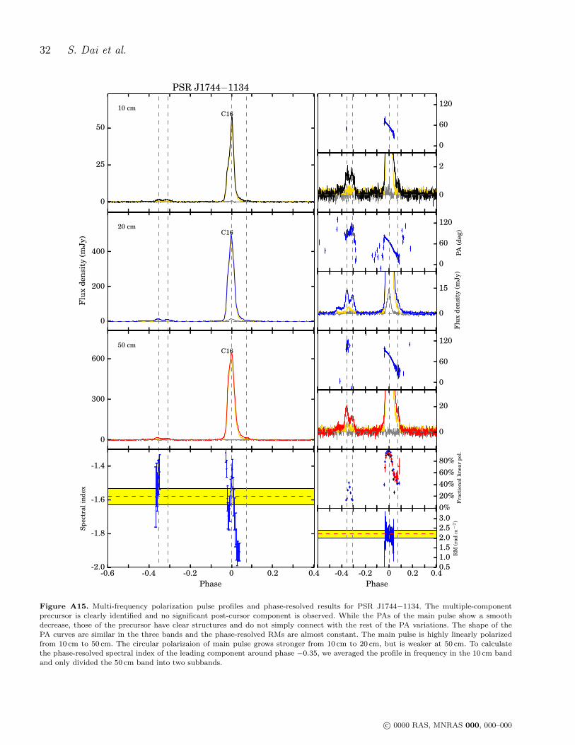
The bottom parts of the right-side panels of Fig. A1 toA24 show the phase-resolved fractional linear polarizationfor each MSP. For most of our MSPs, the phase-resolvedfractional linear polarization is remarkably similar at dif-ferent observing bands (examples include PSR J0437−4715and J1857+0943). However, for a few pulsars (such asPSR J1022+1001) the fractional linear polarization differsbetween bands. We find no strong correlation between thephase-resolved spectral index and the fractional linear polar-ization. In pulsars such as PSRs J1603−7202, J1730−2304,J1939+2134, J2145−0750 and J2241−5236 we see evidencethat the main component has a lower fractional linear po-larization than leading or trailing components (e.g., Basuet al. 2015). However, for PSR J1744−1134, we do not seehigh fractional linear polarizations in the precursor pulse.

At phase ranges where a PA transition occurs, the frac-tional linear polarization is significantly lower than otherphase ranges, which can be explained as the overlap of or-thogonal modes. However, we do not see significantly loweror higher fractional net circular polarization close to PAtransitions. We do not find strong relations between the sizeof the PA transition and the fractional linear polarization.Orthogonal mode transitions normally correspond to lowerfractional linear polarization, but we also see low fractionallinear polarizations for non-orthogonal transitions, for in-stance in PSRs J1045−4509 and J1730−2304.

In Fig. 3, the distribution of phase-resolved fractionallinear, circular and net circular polarization for 24 MSPs in

c© 0000 RAS, MNRAS 000, 000–000

A Study of Multi-frequency Polarization Pulse Profiles of Millisecond Pulsars 11

0.0

0.05

0.110 cm

0.0

0.05

0.1

Norm

alizednumbers

20 cm

0 20 40 60 80 100

〈L〉/S (per cent)

0.0

0.05

0.150 cm

0.0

0.05

0.1

0.15

0.2 10 cm

0.0

0.05

0.1

0.15

0.2 20 cm

-80 -40 0 40 80

〈V 〉/S (per cent)

0.0

0.05

0.1

0.15

0.2 50 cm

0.0

0.1

0.2

0.3 10 cm

0.0

0.1

0.2

0.3 20 cm

0 20 40 60 80 100

〈|V |〉/S (per cent)

0.0

0.1

0.2

0.3 50 cm

Figure 3. Histograms of the phase-resolved fractional linear, net circular and absolute circular polarization for 24 MSPs in three bands.

three bands are shown. To obtain the phase-resolved values,we rebinned the profile in each band into 128 phase bins andonly phase bins whose linear or circular polarization exceedsthree times their baseline rms noise were used. While thedistributions of the fractional linear polarization are sim-ilar across three bands, we see that both the distributionof fractional net circular and absolute circular polarizationbecomes narrower at lower frequencies. This indicates thatthe fractional circular and net circular polarization decreasewith decreasing frequency.

4.4 Rotation measures

With the aligned, three-band profiles, we can not only de-termine new RM values, but also investigate whether thepolarization PAs obey the expected λ2 law. To gain enoughS/N, we typically split the 10 cm and 20 cm bands into foursubbands and the 50 cm band into three subbands. For pul-sars whose linear polarization is weak and has low S/N, wesplit the bands into fewer subbands or fully average themin frequency (specific comments are given in the footnotesof Table 9). For PSR J1832−0836, the S/N of profile is lowand the linear polarization is weak in both 10 cm and 50 cmbands, therefore we excluded it from our RM measurements.

As the PAs vary significantly with pulse phase and alsowith observing frequency, we have selected small regions inpulse phase in which the PAs are generally stable acrossthe three bands. Phase ranges we used for each pulsar arelisted in the third column of Table 9. In order to avoid lowS/N regions and obtain smaller uncertainties of the PA, only

phase bins whose linear polarization exceeds five times thebaseline rms noise were used.

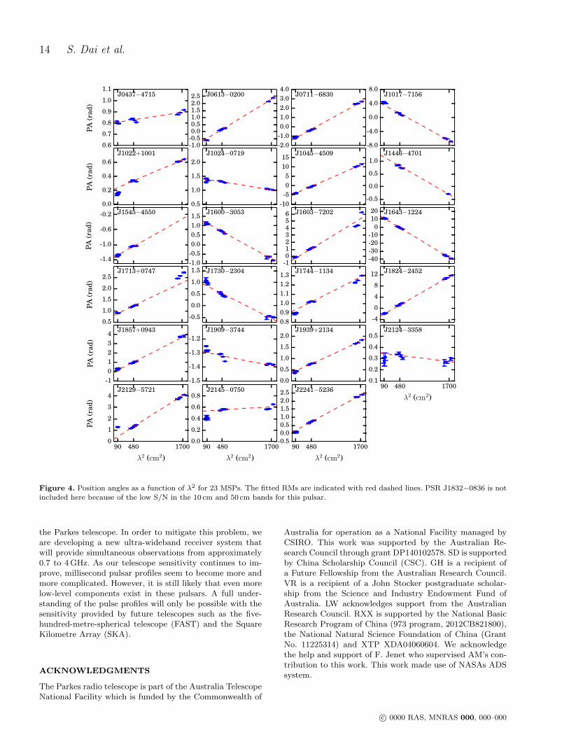
Our results are summarised in Table 9. Previously pub-lished results, obtained from the 20 cm band alone, areshown in the second column. In columns 3, 4 and 5 wepresent our results determined across two bands (10-20, 10-50 and 20-50 respectively). In column 6 we present the RMvalue obtained by fitting across all three bands. In Fig. 4,the mean PAs in the stable regions for each pulsar are plot-ted a function of λ2. The best fitted RMs are indicated withred dashed lines.

For some pulsars, our RMs are significantly differentfrom previously published results. These are explained asfollows. First, previous measurements were obtained usingonly the 20 cm band. In Fig. 4 it is clear that for pulsarssuch as J0437−4715, J1022+1001 and J1744−1134, the PAsin the 20 cm band deviate from the best fitted lines obtainedusing the wider band. Second, previous measurements usedPAs averaged over the pulse longitude while we only aver-aged PAs within phase ranges that PAs are stable. There-fore, the variation of RM across the pulse longitude wouldintroduce deviations.

Fig. 4 shows that, for some pulsars, the PAs gener-ally obey the λ2 fit across a wide range of frequency (e.g.,PSRs J0613−0200, J0711−6830, J1045−4509, J1643−1224,J1824−2452A). However, for other pulsars, the PAs can sig-nificantly deviate from the λ2 fit across bands (e.g., PSRsJ1017−7156, J1713+0747) and show different trends withinbands (e.g., PSRs J0437−4715, J1022+1001, J1730−2304,J1744−1134, J1909−3744, J2124−3358, J2145−0750). ForPSRs J2124−3358 and J2129−5721, the deviation of PA in

c© 0000 RAS, MNRAS 000, 000–000

12 S. Dai et al.

Table 7. The fractional linear polarization 〈L〉/S, the fractional net circular polarization 〈V 〉/S and the fractional absolute circular

polarization 〈|V |〉/S for 24 PPTA MSPs.

PSR 〈L〉/S 〈V 〉/S 〈|V |〉/S50 cm 20 cm 10 cm 50 cm 20 cm 10 cm 50 cm 20 cm 10 cm

(per cent) (per cent) (per cent) (per cent) (per cent) (per cent) (per cent) (per cent) (per cent)

J0437−4715 26.6 ± 0.0 25.1 ± 0.0 20.4 ± 0.0 −4.2 ± 0.0 −2.9 ± 0.0 −8.0 ± 0.0 15.4 ± 0.0 11.3 ± 0.0 12.4 ± 0.0

J0613−0200 28.9 ± 0.3 21.0 ± 0.1 14.7 ± 0.5 −6.5 ± 0.3 5.2 ± 0.1 10.7 ± 0.6 8.9 ± 0.3 5.6 ± 0.1 11.2 ± 0.6

J0711−6830 24.6 ± 0.2 14.1 ± 0.1 17 ± 2 −12.7 ± 0.2 −12.9 ± 0.1 −24 ± 2 12.7 ± 0.2 13.1 ± 0.1 24 ± 2J1017−7156 44.5 ± 0.7 35.4 ± 0.3 42 ± 1 6.9 ± 0.8 −28.9 ± 0.2 −38 ± 2 18.5 ± 0.8 29.5 ± 0.2 42 ± 2

J1022+1001 67.9 ± 0.1 56.3 ± 0.0 23.5 ± 0.2 −13.4 ± 0.1 −11.6 ± 0.0 −2.7 ± 0.2 13.4 ± 0.1 12.6 ± 0.0 5.6 ± 0.2

J1024−0719 69.0 ± 0.6 67.9 ± 0.1 61.7 ± 0.8 1.1 ± 0.6 5.5 ± 0.2 6.1 ± 0.7 3.7 ± 0.6 6.3 ± 0.2 6.7 ± 0.7

J1045−4509 18.7 ± 0.3 22.5 ± 0.1 30.2 ± 0.5 8.2 ± 0.3 14.7 ± 0.1 16.4 ± 0.6 10.6 ± 0.3 16.6 ± 0.1 16.5 ± 0.6

J1446−4701 60.4 ± 2.8 38 ± 1 0.0 ± 3.5 −13 ± 2 −9 ± 1 0.0 ± 3.1 15 ± 3 11 ± 1 0.0 ± 3.1J1545−4550 58 ± 1 59 ± 2 −13.2 ± 0.9 −10 ± 2 17.1 ± 0.9 11 ± 2

J1600−3053 33 ± 2 31.3 ± 0.1 36.8 ± 0.3 0.4 ± 2 3.8 ± 0.1 −2.3 ± 0.3 3 ± 2 4.0 ± 0.1 4.7 ± 0.3

J1603−7202 16.6 ± 0.2 18.6 ± 0.1 31.6 ± 0.7 33.6 ± 0.3 29.0 ± 0.1 15.3 ± 0.8 34.2 ± 0.3 32.4 ± 0.1 22.3 ± 0.8

J1643−1224 20.0 ± 0.3 17.4 ± 0.1 19.9 ± 0.2 6.8 ± 0.2 0.4 ± 0.1 −6.6 ± 0.2 13.9 ± 0.2 13.8 ± 0.1 10.4 ± 0.2J1713+0747 33.3 ± 0.3 31.5 ± 0.0 27.0 ± 0.1 −2.8 ± 0.2 1.1 ± 0.0 −1.1 ± 0.1 3.9 ± 0.2 3.8 ± 0.0 3.8 ± 0.1

J1730−2304 26.2 ± 0.3 29.2 ± 0.1 44.9 ± 0.2 −19.1 ± 0.3 −19.4 ± 0.1 −11.9 ± 0.2 19.2 ± 0.3 20.6 ± 0.1 15.9 ± 0.2

J1744−1134 88.9 ± 0.4 91.8 ± 0.1 88.0 ± 0.4 0.2 ± 0.4 2.9 ± 0.1 1.5 ± 0.3 0.7 ± 0.4 2.9 ± 0.1 1.6 ± 0.3

J1824−2452A 70.9 ± 0.5 77.8 ± 0.2 84.2 ± 1.0 0.1 ± 0.3 3.5 ± 0.2 −0.8 ± 0.8 3.8 ± 0.3 4.4 ± 0.2 5.5 ± 0.8

J1832−0836 36 ± 2 43 ± 11 3 ± 1 −4 ± 10 10 ± 1 11 ± 10J1857+0943 20.9 ± 0.9 14.5 ± 0.1 14.1 ± 0.4 −1.2 ± 0.7 2.5 ± 0.1 0.3 ± 0.4 4.7 ± 0.7 5.8 ± 0.1 7.3 ± 0.4

J1909−3744 61.2 ± 0.4 48.7 ± 0.1 26.3 ± 0.2 13.1 ± 0.4 14.9 ± 0.1 5.0 ± 0.2 15.4 ± 0.4 16.1 ± 0.1 6.6 ± 0.2

J1939+2134 38.1 ± 0.1 30.0 ± 0.0 24.3 ± 0.2 0.9 ± 0.1 3.3 ± 0.0 −0.2 ± 0.2 1.1 ± 0.1 3.3 ± 0.0 1.2 ± 0.2

J2124−3358 46.2 ± 0.2 33.1 ± 0.1 49 ± 1 −2.5 ± 0.2 0.4 ± 0.1 −3.9 ± 1.0 3.8 ± 0.2 5.5 ± 0.1 7 ± 1J2129−5721 66.8 ± 0.6 47.3 ± 0.2 39 ± 8 −27.0 ± 0.6 −24.8 ± 0.2 −16 ± 8 35.5 ± 0.6 26.6 ± 0.2 17 ± 8

J2145−0750 19.2 ± 0.1 15.9 ± 0.0 10.9 ± 0.1 5.9 ± 0.1 9.2 ± 0.0 0.9 ± 0.1 9.5 ± 0.1 10.0 ± 0.0 8.1 ± 0.1

J2241−5236 20.0 ± 0.2 12.6 ± 0.1 12.5 ± 0.7 −2.9 ± 0.2 −0.7 ± 0.1 −4.2 ± 0.7 4.7 ± 0.2 6.2 ± 0.1 8.9 ± 0.7

the 10 cm band from the best fitted result is likely causedby the low S/N of the profile. For PSRs J1603−7202 andJ2145−0750, the PA curves vary dramatically within bandsand cause the deviation of PAs from the λ2 fit.

The bottom parts of the right-side panels of Fig. A1 toA24 show measurements of apparent RM measured at spe-cific phases for each MSP. Since only phase bins whose linearpolarization exceeds five times the baseline rms noise wereused, and we only plot RMs whose uncertainty is smallerthan 3 rad m−2, the phase-resolved RMs only cover pulsephases where the linear polarization is strong and PAs gener-ally obey the λ2 fit. For most pulsars, we can see systematicRM variations across the pulse longitude following the struc-ture of the mean profile. For instance, in PSR J0437−4715the RM shows complex variations from approximately−8 rad m−2 to 8 rad m−2. For PSR J1643−1224, one lin-ear polarization component has a RM of approximately−306 rad m−2 and the other −300 rad m−2. We find thatin some cases significant RM variations are associated withorthogonal or non-orthogonal mode transitions in PA (e.g.,PSRs J1022+1001, J1600−3053, J1643−1224, J1713+0747).For PSR J1744−1134, whose PA curve is smooth across themain pulse, the RMs show minor variations. This is con-sistent with previous phase-resolved RM study of normalpulsars, which also shows that the greatest RM fluctuationsseem coincident with the steepest gradients of the PA curve,whereas pulsars with flat PA curve show little RM varia-tion (Noutsos et al. 2009).

5 SUMMARY OF RESULTS ANDCONCLUSIONS

Our results indicate that:

• Most MSPs in our sample have very wide profiles withmultiple components. This is not a surprise and has beenpresented in numerous earlier publications. We have shownthat 18 of the 24 MSPs exhibit emission over more thanhalf of the pulse period and the overall pulse width is rel-atively constant for pulsars that have high S/N profiles inall three bands. The MSPs in our sample do not show thefrequency evolution of the component separations (Krameret al. 1999a) that has been observed in normal pulsars (e.g.,Cordes 1978; Thorsett 1991; Mitra & Rankin 2002; Mitra &Li 2004; Chen & Wang 2014).

• The spectra for some of the pulsars in our sample signif-icantly deviate from a single power-law across the differentobserving bands. We have observed the spectral steepeningat high frequencies and, for some pulsars, we have shownpositive spectral indices in the 50 cm band. We have also ob-served the spectral flattening within bands at high frequen-cies for PSRs J1022+1001 and J2241−5236. The spectralsteepening and turnover have been identified in normal pul-sars (e.g., Maron et al. 2000; Kijak et al. 2011). The flatten-ing or turn-up of the spectrum has been previously observedat extremely high frequencies (∼ 30 GHz) (Kramer et al.1996), and has been explained by refraction effects (Petrova2002). However, such spectral features have not been ob-

c© 0000 RAS, MNRAS 000, 000–000

A Study of Multi-frequency Polarization Pulse Profiles of Millisecond Pulsars 13

Table 8. The fractional amount of Stokes Q and U and the fractional linear polarization 〈LC〉/S for 24 PPTA MSPs.

PSR 〈Q〉/S 〈U〉/S 〈LC〉/S50 cm 20 cm 10 cm 50 cm 20 cm 10 cm 50 cm 20 cm 10 cm

(per cent) (per cent) (per cent) (per cent) (per cent) (per cent) (per cent) (per cent) (per cent)

J0437−4715 −3.0 ± 0.0 −1.8 ± 0.0 0.2 ± 0.0 0.7 ± 0.0 −4.3 ± 0.0 0.9 ± 0.0 3.0 ± 0.0 4.7 ± 0.0 0.9 ± 0.0J0613−0200 9.9 ± 0.3 8.9 ± 0.1 6.1 ± 0.4 −6.9 ± 0.3 8.3 ± 0.1 −3.1 ± 0.4 12.1 ± 0.3 12.1 ± 0.1 6.8 ± 0.4

J0711−6830 −14.1 ± 0.2 −6.2 ± 0.1 −1.0 ± 0.3 7.0 ± 0.1 −1.0 ± 0.1 0.6 ± 0.3 15.7 ± 0.2 6.3 ± 0.1 1.2 ± 0.3

J1017−7156 23.6 ± 0.7 −17.9 ± 0.2 −22.2 ± 1.2 −22.2 ± 0.7 22.3 ± 0.3 31.2 ± 1.3 32.4 ± 0.7 28.6 ± 0.3 38.4 ± 1.3J1022+1001 14.6 ± 0.1 28.5 ± 0.0 18.1 ± 0.2 22.7 ± 0.1 8.4 ± 0.1 −0.5 ± 0.2 27.0 ± 0.1 29.7 ± 0.1 18.1 ± 0.2

J1024−0719 −20.8 ± 0.5 −49.3 ± 0.1 −30.6 ± 0.4 42.1 ± 0.5 27.4 ± 0.1 14.9 ± 0.5 47.0 ± 0.5 56.4 ± 0.1 34.1 ± 0.5J1045−4509 −6.9 ± 0.2 8.6 ± 0.1 0.2 ± 0.4 −9.6 ± 0.3 −8.7 ± 0.1 −14.6 ± 0.4 11.8 ± 0.3 12.2 ± 0.1 14.6 ± 0.4

J1446−4701 34.6 ± 2.1 1.7 ± 1.0 6.6 ± 4.2 −36.2 ± 2.2 28.8 ± 0.9 12.3 ± 4.1 50.1 ± 2.2 28.8 ± 0.9 14.0 ± 4.1

J1545−4550 −14.9 ± 0.8 −40.3 ± 1.7 −32.5 ± 0.6 −12.4 ± 1.5 35.7 ± 0.7 42.2 ± 1.7J1600−3053 −4.4 ± 0.9 −5.7 ± 0.1 2.1 ± 0.3 −18.0 ± 1.0 −5.3 ± 0.1 −16.0 ± 0.3 18.5 ± 1.0 7.8 ± 0.1 16.1 ± 0.3

J1603−7202 −3.5 ± 0.2 −2.5 ± 0.1 −10.0 ± 0.5 −3.1 ± 0.3 0.4 ± 0.1 0.5 ± 0.5 4.7 ± 0.2 2.5 ± 0.1 10.0 ± 0.5

J1643−1224 12.9 ± 0.2 2.3 ± 0.1 4.5 ± 0.2 −5.3 ± 0.2 −2.7 ± 0.1 0.6 ± 0.2 14.0 ± 0.2 3.5 ± 0.1 4.5 ± 0.2

J1713+0747 −9.4 ± 0.3 −2.9 ± 0.0 −2.0 ± 0.1 11.9 ± 0.3 4.2 ± 0.0 6.0 ± 0.1 15.2 ± 0.3 5.1 ± 0.0 6.4 ± 0.1J1730−2304 9.4 ± 0.2 −11.6 ± 0.1 −19.0 ± 0.2 13.3 ± 0.3 19.3 ± 0.1 18.2 ± 0.2 16.3 ± 0.3 22.5 ± 0.1 26.3 ± 0.2

J1744−1134 −70.5 ± 0.4 −48.7 ± 0.1 −28.7 ± 0.3 34.8 ± 0.4 67.7 ± 0.1 69.3 ± 0.4 78.6 ± 0.4 83.4 ± 0.1 75.0 ± 0.4

J1824−2452A −34.7 ± 0.5 −19.0 ± 0.2 −33.9 ± 0.9 26.8 ± 0.4 43.2 ± 0.1 35.3 ± 0.6 43.8 ± 0.5 47.2 ± 0.1 48.9 ± 0.8

J1832−0836 −1.2 ± 0.9 −15.4 ± 2.1 2.8 ± 0.8 −8.8 ± 2.2 3.1 ± 0.8 17.7 ± 2.1

J1857+0943 2.0 ± 0.5 0.3 ± 0.1 0.3 ± 0.3 0.9 ± 0.4 −0.6 ± 0.1 4.8 ± 0.3 2.2 ± 0.5 0.6 ± 0.1 4.8 ± 0.3J1909−3744 −54.0 ± 0.4 −42.9 ± 0.1 −23.5 ± 0.3 −12.9 ± 0.4 −15.1 ± 0.1 −9.9 ± 0.2 55.5 ± 0.4 45.4 ± 0.1 25.5 ± 0.3

J1939+2134 −30.5 ± 0.1 2.0 ± 0.0 0.1 ± 0.2 −11.8 ± 0.1 16.2 ± 0.0 −6.9 ± 0.2 32.7 ± 0.1 16.3 ± 0.0 6.9 ± 0.2

J2124−3358 19.4 ± 0.1 9.0 ± 0.1 −2.0 ± 0.4 8.2 ± 0.2 10.6 ± 0.1 5.4 ± 0.5 21.1 ± 0.2 13.9 ± 0.1 5.8 ± 0.5

J2129−5721 22.2 ± 0.5 −24.4 ± 0.2 −3.1 ± 2.1 45.1 ± 0.5 29.6 ± 0.2 16.4 ± 2.2 50.2 ± 0.5 38.3 ± 0.2 16.7 ± 2.2J2145−0750 −5.9 ± 0.1 −2.0 ± 0.0 2.5 ± 0.1 6.2 ± 0.1 3.2 ± 0.0 2.3 ± 0.1 8.6 ± 0.1 3.8 ± 0.0 3.3 ± 0.1

J2241−5236 7.8 ± 0.2 0.4 ± 0.1 8.5 ± 0.7 −14.2 ± 0.2 5.0 ± 0.1 −3.8 ± 0.7 16.2 ± 0.2 5.0 ± 0.1 9.3 ± 0.7

served in MSPs before, and previous measurements of MSPflux densities over a wide frequency range did not show spec-tral turnovers or breaks (Kramer et al. 1999a; Kuzmin &Losovsky 2001).

• For almost all of the MSPs in our sample, the ob-served three-band PA variations across the profile are ex-tremely complicated and cannot be fitted using the RVM.We show complex details of the PA variation for sev-eral MSPs, which were previously thought to have rela-tively flat or smooth PA profiles (e.g., PSRs J1024−0719,J1600−3053, J1744−1134, J2124−3358). Across bands, thePA profiles can evolve significantly (e.g., PSRs J0437−4715,J0711−6830, J1603−7202, J1730−2304).

One exception is PSR J1022+1001, whose PA profile isrelatively smooth in all three bands except for a discontinu-ity close to phase zero. At 10 cm, the PA variation fits theRVM very well. The PA variation departs from the RVMprogressively with decreasing frequency. One model to ex-plain this would be that at higher frequencies and loweremission heights, the magnetic field is closer to a simpledipolar field. As the frequency decreases, the magnetic fielddeparts from this simple dipolar form. It is worth notingthat PSR J1022+1001 has the longest pulse period of thepulsars in our sample.

• We have observed systematic variations of apparent RMacross the pulse longitude following the structure of themean profile, indicating that such variations are likely toarise from the pulsar magnetosphere. We have also shownthat the PA of some pulsars does not follow the λ2 relation.

As discussed in Noutsos et al. (2009), possible explanationsof these phenomena includes Faraday rotation in the pul-sar magnetosphere (Kennett & Melrose 1998; Wang et al.2011), the superposition and frequency dependence of quasi-orthogonal polarization modes (Ramachandran et al. 2004)and interstellar scattering (Karastergiou 2009).

• Different pulse components usually have differing spec-tral indices, apparent RMs and fractional polarizations.Measurements of flux density as a function of frequencyfor individual components can significantly differ from thatobtained by averaging over the entire profile. The spectralshape also often deviates from a single power-law. In somecases, the peaks of pulse components coincide with the lo-cal maximum or minimum of the phase-resolved spectralindex. The fractional polarization increases with increasingfrequency for some components, but decreases for other com-ponents. These results suggest that there are multiple emis-sion regions or structures within the pulsar magnetosphereand that pulse components originate in different locationswithin the magnetosphere (e.g., Dyks et al. 2010).

The main goal of this paper has been to inspire andpromote our studies and understanding of the MSP emis-sion mechanism by publishing high quality, multi-frequencypolarization profiles. All the raw data and resulting averagedprofiles are available for public access online.

Producing a model to describe all these observationswill be extremely challenging and made more-so by the gapsin the frequency coverage that we currently have available at

c© 0000 RAS, MNRAS 000, 000–000

14 S. Dai et al.

0.6

0.7

0.8

0.9

1.0

1.1PA(rad)

J0437−4715

-1.0-0.50.00.51.01.52.02.5 J0613−0200

-2.0

-1.0

0.0

1.0

2.0

3.0

4.0J0711−6830

-8.0

-4.0

0.0

4.0

8.0J1017−7156

0.0

0.2

0.4

0.6

PA(rad)

J1022+1001

0.5

1.0

1.5

2.0

J1024−0719

-10

-5

0

5

10

15J1045−4509

-0.5

0.0

0.5

1.0

J1446−4701

-1.4

-1.0

-0.6

-0.2

PA(rad)

J1545−4550

-1.0

-0.5

0.0

0.5

1.0

1.5J1600−3053

-10

123

456 J1603−7202

-40

-30

-20

-10

0

10

20 J1643−1224

0.5

1.0

1.5

2.0

2.5

PA(rad)

J1713+0747

-0.5

0.0

0.5

1.0

1.5 J1730−2304

0.8

0.9

1.0

1.1

1.2

1.3J1744−1134

-4

0

4

8

12J1824−2452

-1

0

1

2

3

4

PA(rad)

J1857+0943

-1.5

-1.4

-1.3

-1.2

J1909−3744

0.0

0.5

1.0

1.5

2.0J1939+2134

90 480 1700

λ2 (cm2)

0.1

0.2

0.3

0.4

0.5J2124−3358

90 480 1700

λ2 (cm2)

0

1

2

3

4

PA(rad)

J2129−5721

90 480 1700

λ2 (cm2)

0.0

0.2

0.4

0.6

0.8J2145−0750

90 480 1700

λ2 (cm2)

-0.5

0.0

0.5

1.0

1.5

2.0

2.5 J2241−5236

Figure 4. Position angles as a function of λ2 for 23 MSPs. The fitted RMs are indicated with red dashed lines. PSR J1832−0836 is not

included here because of the low S/N in the 10 cm and 50 cm bands for this pulsar.

the Parkes telescope. In order to mitigate this problem, weare developing a new ultra-wideband receiver system thatwill provide simultaneous observations from approximately0.7 to 4 GHz. As our telescope sensitivity continues to im-prove, millisecond pulsar profiles seem to become more andmore complicated. However, it is still likely that even morelow-level components exist in these pulsars. A full under-standing of the pulse profiles will only be possible with thesensitivity provided by future telescopes such as the five-hundred-metre-spherical telescope (FAST) and the SquareKilometre Array (SKA).

ACKNOWLEDGMENTS

The Parkes radio telescope is part of the Australia TelescopeNational Facility which is funded by the Commonwealth of

Australia for operation as a National Facility managed byCSIRO. This work was supported by the Australian Re-search Council through grant DP140102578. SD is supportedby China Scholarship Council (CSC). GH is a recipient ofa Future Fellowship from the Australian Research Council.VR is a recipient of a John Stocker postgraduate scholar-ship from the Science and Industry Endowment Fund ofAustralia. LW acknowledges support from the AustralianResearch Council. RXX is supported by the National BasicResearch Program of China (973 program, 2012CB821800),the National Natural Science Foundation of China (GrantNo. 11225314) and XTP XDA04060604. We acknowledgethe help and support of F. Jenet who supervised AM’s con-tribution to this work. This work made use of NASAs ADSsystem.

c© 0000 RAS, MNRAS 000, 000–000

A Study of Multi-frequency Polarization Pulse Profiles of Millisecond Pulsars 15

Table 9. Interstellar RMs for 23 MSPs in units of rad m−2. Previoulsy published results without footnotes are from Yan et al. (2011a).

PSR Previously published Phase ranges Measured from mean profile

20 cm 10 cm - 20 cm 10 cm - 50 cm 20 cm - 50 cm fitting

J0437−4715 0.0 ± 0.4 (0.01, 0.03) 0.60± 0.01 0.618± 0.004 0.624± 0.001 0.58± 0.09

J0613−0200? 9.7 ± 1.1 (0.01, 0.03) 19.8± 0.7 17.8± 0.2 17.20± 0.08 17.5± 0.3

J0711−6830 21.6 ± 3.1 (−0.28,−0.26) 22.1± 0.4 23.5± 0.1 23.89± 0.05 23.9± 0.4J1017−7156 −78 ± 3a (−0.025, 0.005) −82.1± 0.2 −66.59± 0.04 −61.66± 0.03 −63± 1

J1022+1001 −0.6 ± 0.5 (−0.01, 0.01) 4.68± 0.06 2.95± 0.01 2.405± 0.004 2.4± 0.1

J1024−0719 −8.2 ± 0.8 (−0.04, 0.03) −1.88± 0.09 −2.26± 0.03 −2.38± 0.02 −2.4± 0.2

J1045−4509 92.0 ± 1.0 (0.05, 0.07) 91.5± 0.1 93.34± 0.06 93.91± 0.07 94.7± 0.7

J1446−4701∗ −14 ± 3a (−0.05, 0.0) −8.98± 0.11 −9.1± 0.2J1545−4550† −0.6 ± 1.3b (−0.05, 0.0) 6.3± 0.2 6.1± 0.5

J1600−3053 −15.5 ± 1.0 (0.01, 0.04) −11.6± 0.1 −11.77± 0.09 −11.8± 0.1 −11.8± 0.3

J1603−7202 27.7 ± 0.8 (−0.01, 0.0) 31.2± 0.4 28.91± 0.09 28.20± 0.05 35± 2

J1643−1224 −308.1 ± 1.0 (−0.1,−0.05) −306.8± 0.2 −301.70± 0.06 −300.09± 0.05 −305.7± 0.2J1713+0747 8.4 ± 0.6 (0.0, 0.01) 8.19± 0.02 10.67± 0.02 11.45± 0.03 8.7± 0.5

J1730−2304 −7.2 ± 2.2 (−0.02, 0.0) −13.4± 0.2 −9.22± 0.08 −7.88± 0.1 −8.8± 0.6

J1744−1134 −1.6 ± 0.7 (0.0, 0.02) 3.24± 0.02 2.34± 0.01 2.05± 0.01 2.2± 0.2

J1824−2452A 77.8 ± 0.6 (−0.02, 0.04) 82.6± 0.3 82.06± 0.07 81.91± 0.04 82.2± 0.2

J1857+0943‡ 16.4 ± 3.5 (0.06, 0.062) 18.4± 0.8 21.4± 0.3 22.4± 0.3 22.2± 0.9J1909−3744 −6.6 ± 0.8 (−0.01, 0.01) −0.38± 0.02 −0.30± 0.01 −0.27± 0.01 −0.6± 0.2

J1939+2134 6.7 ± 0.6 (0.0, 0.04) 12.3± 0.2 9.13± 0.05 8.11± 0.01 8.3± 0.1

J2124−3358 −5.0 ± 0.9 (−0.4,−0.38) 1.6± 0.3 0.07± 0.08 −0.41± 0.03 −0.4± 0.1

J2129−5721q 23.5 ± 0.8 (−0.02, 0.0) 0.00± 0.06 16.61± 0.02 21.88± 0.03 22.3± 0.3

J2145−0750 −1.3 ± 0.7 (−0.03,−0.01) 1.4± 0.3 −0.31± 0.09 −0.85± 0.04 −0.8± 0.1J2241−5236 14 ± 6c (0.02, 0.04) 16.1± 0.3 13.84± 0.08 13.14± 0.04 13.3± 0.1

a Keith et al. (2012); b Burgay et al. (2013); c Keith et al. (2011).? J0613−0200: 50 cm, two subbands; 10 cm, one subband.∗ J1446−4701: 50 cm, one subband; 10 cm, not used.

† J1545−4550: 50 cm, not used.‡ J1857+0943: 50 cm, two subband.q J2129−5721: 10 cm, one subband..

REFERENCES

Abdo A. A. et al., 2009, Science, 325, 848Abdo A. A. et al., 2010, ApJS, 187, 460Abdo A. A. et al., 2013, ApJS, 208, 17Barr E. D. et al., 2013, MNRAS, 429, 1633Basu R., Mitra D., Rankin J. M., 2015, ApJ, 798, 105Bhat N. D. R. et al., 2014, ApJL, 791, L32Burgay M. et al., 2013, MNRAS, 433, 259Chen J. L., Wang H. G., 2014, ApJS, 215, 11Chen J.-L., Wang H.-G., Chen W.-H., Zhang H., Liu Y.,2007, ChJAA, 7, 789

Cordes J. M., 1978, ApJ, 222, 1006Cordes J. M., Shannon R. M., 2010, preprint(arXiv:1010.3785)

Cordes J. M., Shannon R. M., 2012, ApJ, 750, 89Crawford F., Kaspi V. M., Bell J. F., 2000, Astron. J., 119,2376

Dyks J., Rudak B., 2003, ApJ, 598, 1201Dyks J., Rudak B., Demorest P., 2010, MNRAS, 401, 1781Espinoza C. M. et al., 2013, MNRAS, 430, 571Everett J. E., Weisberg J. M., 2001, ApJ, 553, 341Foster R. S., Backer D. C., 1990, ApJ, 361, 300Guillemot L. et al., 2012, ApJ, 744, 33Gupta Y., Gangadhara R. T., 2003, ApJ, 584, 418Han J. L., Manchester R. N., 2001, MNRAS, 320, L35Han J. L., Manchester R. N., Lyne A. G., Qiao G. J., van

Straten W., 2006, ApJ, 642, 868

Hobbs G. et al., 2011, Publications of the AstronomicalSociety of Australia, 28, 202

Hobbs G. B., Edwards R. T., Manchester R. N., 2006, MN-RAS, 369, 655

Hotan A. W., van Straten W., Manchester R. N., 2004,Publications of the Astronomical Society of Australia, 21,302

Johnston S. et al., 1993, Nature, 361, 613

Johnston S., Weisberg J. M., 2006, MNRAS, 368, 1856

Karastergiou A., 2009, MNRAS, 392, L60

Karastergiou A., Johnston S., 2007, MNRAS, 380, 1678

Keith M. J. et al., 2013, MNRAS, 429, 2161

Keith M. J. et al., 2012, MNRAS, 419, 1752

Keith M. J. et al., 2011, MNRAS, 414, 1292

Kennett M., Melrose D., 1998, Publications of the Astro-nomical Society of Australia, 15, 211

Kijak J., Lewandowski W., Maron O., Gupta Y., JessnerA., 2011, A&A, 531, A16

Kramer M., 1994, A&AS, 107, 527

Kramer M., Lange C., Lorimer D. R., Backer D. C., XilourisK. M., Jessner A., Wielebinski R., 1999a, ApJ, 526, 957

Kramer M., Wielebinski R., Jessner A., Gil J. A.,Seiradakis J. H., 1994, A&AS, 107, 515

Kramer M. et al., 1999b, ApJ, 520, 324

Kramer M., Xilouris K. M., Jessner A., Wielebinski R.,

c© 0000 RAS, MNRAS 000, 000–000

16 S. Dai et al.

Timofeev M., 1996, A&A, 306, 867Kramer M., Xilouris K. M., Lorimer D. R., DoroshenkoO., Jessner A., Wielebinski R., Wolszczan A., Camilo F.,1998, ApJ, 501, 270

Kuzmin A. D., Losovsky B. Y., 2001, A&A, 368, 230Liu K. et al., 2014, MNRAS, 443, 3752Lorimer D. R., Yates J. A., Lyne A. G., Gould D. M., 1995,MNRAS, 273, 411

Lyne A. G., Manchester R. N., 1988, MNRAS, 234, 477Manchester R. N., 1995, Journal of Astrophysics and As-tronomy, 16, 107

Manchester R. N., 2005, Ap&SS, 297, 101Manchester R. N., Han J. L., 2004, ApJ, 609, 354Manchester R. N. et al., 2013, Publications of the Astro-nomical Society of Australia, 30, 17

Manchester R. N., Hobbs G. B., Teoh A., Hobbs M., 2005,Astron. J., 129, 1993

Manchester R. N., Johnston S., 1995, ApJL, 441, L65Maron O., Kijak J., Kramer M., Wielebinski R., 2000,A&AS, 147, 195

Michel F. C., 1987, ApJ, 322, 822Mitra D., Li X. H., 2004, A&A, 421, 215Mitra D., Rankin J. M., 2002, ApJ, 577, 322Navarro J., Manchester R. N., Sandhu J. S., Kulkarni S. R.,Bailes M., 1997, ApJ, 486, 1019

Noutsos A., Karastergiou A., Kramer M., Johnston S.,Stappers B. W., 2009, MNRAS, 396, 1559

Ord S. M., van Straten W., Hotan A. W., Bailes M., 2004,MNRAS, 352, 804

Os lowski S., van Straten W., Bailes M., Jameson A., HobbsG., 2014, MNRAS, 441, 3148

Pennucci T. T., Demorest P. B., Ransom S. M., 2014, ApJ,790, 93

Petrova S. A., 2002, A&A, 383, 1067Radhakrishnan V., Cooke D. J., 1969, Astrophys. Lett., 3,225

Ramachandran R., Backer D. C., Rankin J. M., WeisbergJ. M., Devine K. E., 2004, ApJ, 606, 1167

Rankin J. M., 1983, ApJ, 274, 333Ravi V., Manchester R. N., Hobbs G., 2010, ApJL, 716,L85

Shannon R. M. et al., 2014, MNRAS, 443, 1463Shannon R. M. et al., 2013, Science, 342, 334Stairs I. H., Thorsett S. E., Camilo F., 1999, ApJS, 123,627

Taylor J. H., 1992, Royal Society of London PhilosophicalTransactions Series A, 341, 117

Thorsett S. E., 1991, ApJ, 377, 263Thorsett S. E., Stinebring D. R., 1990, ApJ, 361, 644Toscano M., Bailes M., Manchester R. N., Sandhu J. S.,1998, ApJ, 506, 863

van Straten W., 2004, ApJS, 152, 129van Straten W., Manchester R. N., Johnston S., ReynoldsJ. E., 2010, Publications of the Astronomical Society ofAustralia, 27, 104

Wang C., Han J. L., Lai D., 2011, MNRAS, 417, 1183Wang H. G. et al., 2014, ApJ, 789, 73Wang J. B. et al., 2015, MNRAS, 446, 1657Wang N., Manchester R. N., Johnston S., Rickett B., ZhangJ., Yusup A., Chen M., 2005, MNRAS, 358, 270

Watters K. P., Romani R. W., Weltevrede P., Johnston S.,2009, ApJ, 695, 1289

Xilouris K. M., Kramer M., Jessner A., von HoensbroechA., Lorimer D., Wielebinski R., Wolszczan A., Camilo F.,1998, ApJ, 501, 286

Yan W. M. et al., 2011a, MNRAS, 414, 2087Yan W. M. et al., 2011b, Ap&SS, 335, 485Zhu X.-J. et al., 2014, MNRAS, 444, 3709

APPENDIX A: MULTI-FREQUENCYPOLARIZATION PROFILES

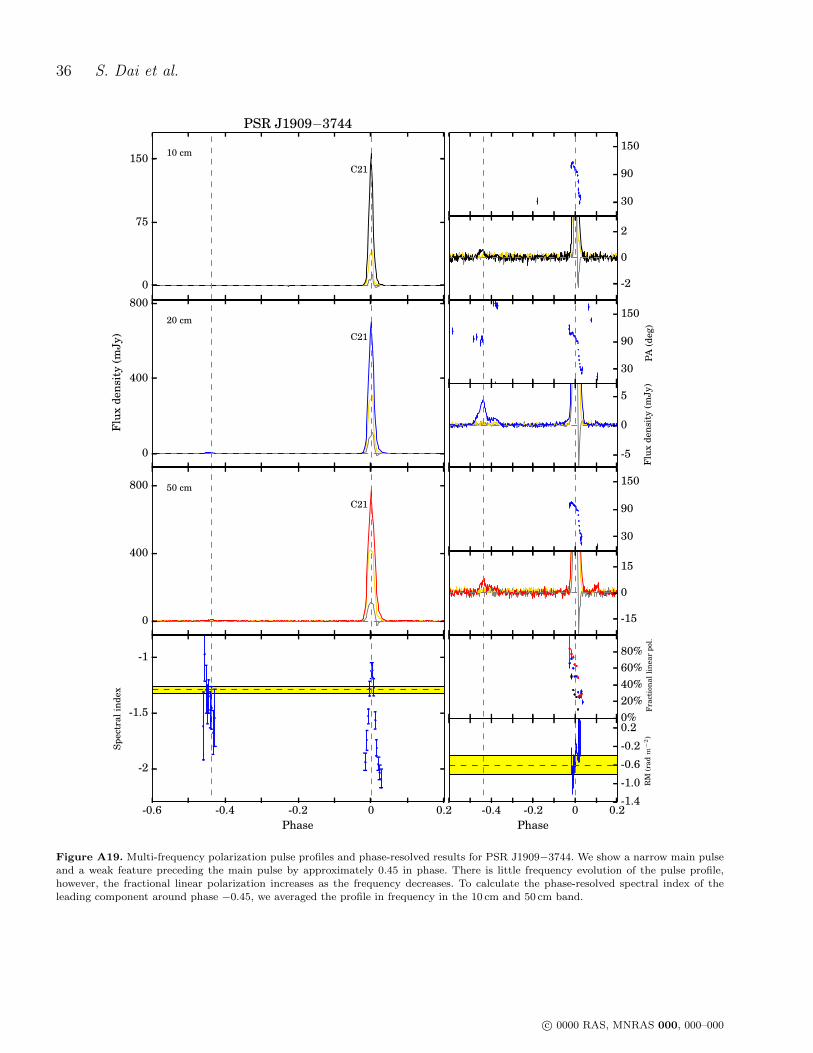
In this section, we present the multi-frequency polarizationpulse profiles and phase-resolved results for each MSP inFigures A1 to A24. The left-hand panels show the pulse pro-file in the 10 cm (top), 20 cm (second panel) and 50 cm (thirdpanel) observing bands. The black, blue and red lines inthese panels respectively indicate the total intensity, StokesI, profile in the three bands. The yellow line indicates lin-ear polarization and the grey line shows circular polariza-tion. The bottom panel on the left-hand side presents thephase-resolved spectral index. The red dashed line and yel-low highlighted region represent the measured spectral indexand its uncertainty as presented in Table 6. In the right-handpanels we have two panels for each of the 10 cm, 20 cm and50 cm bands. The upper panel shows the position angle ofthe linear polarization at the band central frequency (in de-grees). The lower panels shows a zoom-in around the profilebaseline to show weak profile features. The colour scheme isthe same as in the left-hand panels. The bottom two pan-els on the right-hand side show the phase-resolved fractionallinear polarization for the three observing bands using thesame colour scheme as above, and the phase-resolved RM.The red dashed line and yellow highlighted region representthe measured RM value and its uncertainty. In all panels,vertical dashed lines show the positions of peaks in the 20 cmtotal intensity profile.

In Table A1, we give the references, baseline duty cycleand S/N for the pulse profile in each band for each pul-sar. Specific comments for each individual pulsar and on thecomparison with previous work are given in the caption ofeach figure.

c© 0000 RAS, MNRAS 000, 000–000

A Study of Multi-frequency Polarization Pulse Profiles of Millisecond Pulsars 17

Table A1. References, duty cycles and S/N for MSPs in our sample.

PSR References Duty cycle S/N50 cm 20 cm 10 cm

J0437−4715 Johnston et al. (1993); Manchester & Johnston (1995) 0.05 14285.8 33512.4 5445.6

Navarro et al. (1997); Yan et al. (2011a)J0613−0200 Xilouris et al. (1998); Stairs et al. (1999) 0.2 812.3 1490.1 396.5

Ord et al. (2004); Yan et al. (2011a)

J0711−6830 Manchester & Han (2004); Ord et al. (2004); Yan et al. (2011a) 0.05 1194.0 3368.4 488.8J1017−7156 Keith et al. (2012) 0.2 634.4 1057.0 233.6

J1022+1001 Xilouris et al. (1998); Kramer et al. (1999b) 0.2 4827.2 6979.8 1577.0

Stairs et al. (1999); Ord et al. (2004); Yan et al. (2011a)

J1024−0719 Xilouris et al. (1998); Ord et al. (2004); Yan et al. (2011a) 0.05 613.0 1459.8 273.6J1045−4509 Manchester & Han (2004); Ord et al. (2004); Yan et al. (2011a) 0.2 1097.4 2155.7 456.8

J1446−4701 Keith et al. (2012) 0.2 62.2 215.2 31.6

J1545−4550 Burgay et al. (2013) 0.2 203.5 157.8J1600−3053 Ord et al. (2004); Yan et al. (2011a) 0.2 213.6 2158.3 1045.2

J1603−7202 Manchester & Han (2004); Ord et al. (2004); Yan et al. (2011a) 0.2 1603.6 3215.6 446.8J1643−1224 Xilouris et al. (1998); Stairs et al. (1999) 0.2 1505.3 3097.7 1073.4

Ord et al. (2004); Yan et al. (2011a)

J1713+0747 Xilouris et al. (1998); Stairs et al. (1999) 0.2 1751.4 10294.1 3894.0Ord et al. (2004); Yan et al. (2011a)

J1730−2304 Xilouris et al. (1998); Kramer et al. (1998) 0.2 1138.4 2645.2 1665.1

Stairs et al. (1999); Ord et al. (2004); Yan et al. (2011a)J1744−1134 Xilouris et al. (1998); Kramer et al. (1998) 0.2 1808.5 4516.1 1025.0

Stairs et al. (1999); Ord et al. (2004); Yan et al. (2011a)

J1824−2452A Ord et al. (2004); Yan et al. (2011a); Stairs et al. (1999) 0.05 432.2 620.0 136.3

J1832−0836 Burgay et al. (2013) 0.2 100.8 24.2J1857+0943 Thorsett & Stinebring (1990); Xilouris et al. (1998) 0.2 376.7 1563.0 498.9

Ord et al. (2004); Yan et al. (2011a)

J1909−3744 Ord et al. (2004); Yan et al. (2011a) 0.2 1702.4 9413.7 1971.3J1939+2134 Thorsett & Stinebring (1990); Xilouris et al. (1998) 0.2 2066.5 1562.6 565.0

Stairs et al. (1999); Ord et al. (2004); Yan et al. (2011a)

J2124−3358 Manchester & Han (2004); Ord et al. (2004); Yan et al. (2011a) 0.05 332.2 411.0 135.4

J2129−5721 Manchester & Han (2004); Ord et al. (2004); Yan et al. (2011a) 0.2 750.6 1829.3 59.5

J2145−0750 Xilouris et al. (1998); Stairs et al. (1999) 0.2 4051.6 8680.7 1483.6Manchester & Han (2004); Ord et al. (2004); Yan et al. (2011a)

J2241−5236 Keith et al. (2011) 0.2 4270.2 3549.0 311.0

c© 0000 RAS, MNRAS 000, 000–000

18 S. Dai et al.

0

0.6

1.2

10 cm

PSR J0437−4715

0

1

2

3

Fluxdensity

(Jy)

20 cm

0

4

8 50 cm

-0.4 -0.2 0 0.2 0.4

Phase

-2

-1

Spectralindex

40

100

160

-40

0

40

-90

0

90

PA

(deg)

-150

0

150

Fluxdensity

(mJy)

-60

20

100

-1000

0

1000

0%

20%

40%

60%

80%Fractionallinearpol.

-0.4 -0.2 0 0.2 0 4

Phase

-4

0

4

8

RM

(radm

−2)

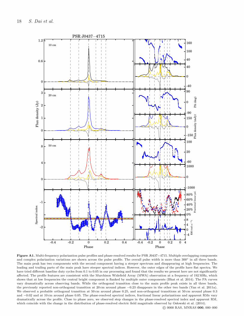
Figure A1. Multi-frequency polarization pulse profiles and phase-resolved results for PSR J0437−4715. Multiple overlapping components

and complex polarization variations are shown across the pulse profile. The overall pulse width is more than 300◦ in all three bands.The main peak has two components with the second component having a steeper spectrum and disappearing at high frequencies. Theleading and trailing parts of the main peak have steeper spectral indices. However, the outer edges of the profile have flat spectra. We

have tried different baseline duty cycles from 0.1 to 0.05 in our processing and found that the results we present here are not significantlyaffected. The profile features are consistent with the Murchison Widefield Array (MWA) observation at a frequency of 192 MHz, which

shows that at low frequencies the central bright component is flanked by multiple outer components (Bhat et al. 2014). The PA curvesvary dramatically across observing bands. While the orthogonal transition close to the main profile peak exists in all three bands,the previously reported non-orthogonal transition at 20 cm around phase −0.23 disappears in the other two bands (Yan et al. 2011a).

We observed a probable orthogonal transition at 50 cm around phase 0.25, and non-orthogonal transitions at 50 cm around phase 0.3

and −0.02 and at 10 cm around phase 0.05. The phase-resolved spectral indices, fractional linear polarizations and apparent RMs varydramatically across the profile. Close to phase zero, we observed step changes in the phase-resolved spectral index and apparent RM,

which coincide with the change in the distribution of phase-resolved electric field magnitude observed by Os lowski et al. (2014).

c© 0000 RAS, MNRAS 000, 000–000

A Study of Multi-frequency Polarization Pulse Profiles of Millisecond Pulsars 19

0

4

8 10 cm

PSR J0613−0200

0

10

20

Fluxdensity

(mJy)

20 cm

0

50

100 50 cm

-0.2 0 0.2 0.4

Phase

-3

-2

-1

Spectralindex

-60

0

60

-1

0

1

-60

20

100

PA

(deg)

-1

0

1

Fluxdensity

(mJy)

0

60

120

-15

0

15

0%

20%

40%

60%

80%Fractionallinearpol.

-0.2 0 0.2 0.4

Phase

10

15

20

RM

(radm

−2)

Figure A2. Multi-frequency polarization pulse profiles and phase-resolved results for PSR J0613−0200. Our high S/N profiles provide

more details in the PA curve compared to previous observations, and we show that the PA curves are complex and very different in threebands. At 20 cm, the discontinuous PA at the leading edge of the trailing component reported by Yan et al. (2011a) is not observed, andthe PA curve seems to be continuous. The main pulse of the profile shows clear frequency evolution, and most significantly, the trailingpeak has a very steep spectrum. The trailing peak splits into two peaks at low frequencies as previously observed by Stairs et al. (1999).

From the high frequencies to low frequencies, the fractional linear polarization increases, and the trailing component becomes highlylinearly polarized. At 50 cm, the circular polarization swaps sign compared to higher frequencies. The three main pulse components ofthe profile clearly have different apparent RMs.

c© 0000 RAS, MNRAS 000, 000–000

20 S. Dai et al.

0

5

10 10 cm

C1

C2

PSR J0711−6830

0

50

100

150

Fluxdensity

(mJy)

20 cm

C1

C2

0

100

200 50 cm

C1

C2

-0.4 -0.2 0 0.2 0.4

Phase

-2.5

-2

-1.5

Spectralindex

45

135

-1

0

1

45

135

PA

(deg)

-20

0

20

Fluxdensity

(mJy)

45

135

-20

0

20

0%

20%

40%

60%

80%Fractionallinearpol.

-0.4 -0.2 0 0.2 0.4

Phase

20

22

24

26

RM

(radm

−2)

Figure A3. Multi-frequency polarization pulse profiles and phase-resolved results for PSR J0711−6830. The double-peaked weak com-

ponent following the second peak is clear. The orthogonal mode transition after the peak of the leading component seen by Yan et al.(2011a) is confirmed at 20 cm and is seen at 50 cm. However the orthogonal mode transition near the trailing edge of the main peak isnot present at 50 cm. The leading component has a slightly steeper spectrum than the main pulse. The fractional linear polarization ofthe main peak decreases significantly with increasing frequency.

c© 0000 RAS, MNRAS 000, 000–000

A Study of Multi-frequency Polarization Pulse Profiles of Millisecond Pulsars 21

0

7.5

1510 cm

C3

PSR J1017−7156

0

20

40

Fluxdensity

(mJy)

20 cm

C3

0

30

60

50 cm

C3

-0.2 -0.1 0 0.1 0.2

Phase

-2

-1.5

-1

Spectralindex

20

60

100

-2

0

2

30

90

150

PA

(deg)

-6

0

6

Fluxdensity

(mJy)

-80

-40

0

-10

0

10

0%

20%

40%

60%

80%Fractionallinearpol.

-0.2 -0.1 0 0.1 0.2

Phase

-70

-66

-62

-58

RM

(radm

−2)

Figure A4. Multi-frequency polarization pulse profiles and phase-resolved results for PSR J1017−7156. We show that the PA variations

are more complex than was observed in previous work. While the leading and trailing edges of the main pulse have a steeper spectrumcompared with the central peak, the trailing component around phase 0.04 has a much flatter spectrum. Both the linear and circularpolarization have multiple components and show significant evolution with frequency. Especially, the circular polarization of the mainpulse seems to consist of two components of opposite sign with the left-circular component having narrower width and much steeper

spectrum.

c© 0000 RAS, MNRAS 000, 000–000

22 S. Dai et al.

0

20

40 10 cm C4

C5

PSR J1022+1001

0

100

200

Fluxdensity

(mJy)

20 cmC4

C5

0

1500

300050 cm

C4

C5

-0.3 -0.2 -0.1 0 0.1

Phase

-2.5

-2

-1.5

-1

Spectralindex

0

90

180

-4

0

4

0

90

180

PA

(deg)

-50

0

50

Fluxdensity

(mJy)

0

90

180

-500

0

500

0%

20%

40%

60%

80%Fractionallinearpol.

-0.3 -0.2 -0.1 0 0.1 0.2

Phase

0

2

4

6

8

RM

(radm

−2)

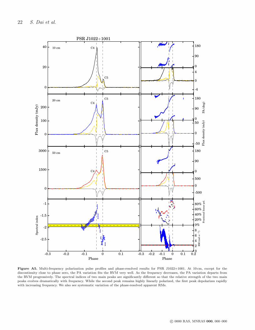
Figure A5. Multi-frequency polarization pulse profiles and phase-resolved results for PSR J1022+1001. At 10 cm, except for the

discontinuity close to phase zero, the PA variation fits the RVM very well. As the frequency decreases, the PA variation departs fromthe RVM progressively. The spectral indices of two main peaks are significantly different so that the relative strength of the two mainpeaks evolves dramatically with frequency. While the second peak remains highly linearly polarized, the first peak depolarizes rapidlywith increasing frequency. We also see systematic variation of the phase-resolved apparent RMs.

c© 0000 RAS, MNRAS 000, 000–000

A Study of Multi-frequency Polarization Pulse Profiles of Millisecond Pulsars 23

0

2.5

510 cm C6

C7

PSR J1024−0719

0

20

40

Fluxdensity

(mJy)

20 cm C6

C7

0

75

150 50 cm C6

C7

-0.4 -0.2 0 0.2 0.4

Phase

-2

-1.5

Spectralindex

90

180

-0.5

0

0.5

90

180

PA

(deg)

-2

0

2

Fluxdensity

(mJy)

90

180

-10

0

10

0%

20%

40%

60%

80%Fractionallinearpol.

-0.4 -0.2 0 0.2 0.4

Phase

-4

-3

-2

-1

0

RM

(radm

−2)

Figure A6. Multi-frequency polarization pulse profiles and phase-resolved results for PSR J1024−0719. Besides the flat PA curve across

the main part of the profile as previously reported, we also show the PAs of the trailing component which increase with phase at 20 cmand 50 cm. The leading component and the trailing component of the profile have much steeper spectra compared with the central peaks.The leading part of the profile is highly linearly polarized and has stable phase-resolved RMs. As the fractional linear polarization dropsdown at the trailing part, the RMs show some variations.

c© 0000 RAS, MNRAS 000, 000–000

24 S. Dai et al.

0

2.5

5

10 cm

PSR J1045−4509

0

15

30

Fluxdensity

(mJy)

20 cm

0

50

100 50 cm

-0.6 -0.4 -0.2 0 0.2

Phase

-2.5

-2

Spectralindex

-60

0

60

-0.5

0

0.5

-60

0

60

PA

(deg)

-1

0

1

Fluxdensity

(mJy)

-60

0

60

-6

0

6

0%

20%

40%

60%

80%Fractionallinearpol.

-0.6 -0.4 -0.2 0 0.2

Phase

88

90

92

94

96

98

RM

(radm

−2)

Figure A7. Multi-frequency polarization pulse profiles and phase-resolved results for PSR J1045−4509. We confirm that the leading

emission is joined to the main pulse by a low-level bridge of emission as seen by Yan et al. (2011a). We show the complex PA curve withmore detail, and determine the PA of the low-level bridge connecting the leading emission and the main pulse. At the leading edge of themain pulse, there is a non-orthogonal transition rather than an orthogonal transition as suggested by Yan et al. (2011a). Around phasezero, a non-orthogonal transition can be seen in all three bands. The PA of the low-level bridge emission seems to be discontinuous with

the other PA variations and could be an orthogonal mode. To calculate the phase-resolved spectral index of the leading emission, weaveraged the profile in frequency in the 10 cm band and only divided the 50 cm band into two subbands. We show that the leading edgeof the main pulse has a steeper spectrum than that of the trailing edge. We also see an increase in the linear polarization of the trailing

edge of the main pulse at high frequencies.

c© 0000 RAS, MNRAS 000, 000–000

A Study of Multi-frequency Polarization Pulse Profiles of Millisecond Pulsars 25

0

5

10

10 cm

PSR J1446−4701

0

7.5

15

Fluxdensity

(mJy)

20 cm

0

20

4050 cm

-0.4 -0.2 0 0.2 0.4

Phase

-2.5

-2

-1.5

Spectralindex

0

45

90

-2

0

2

0

45

90

PA

(deg)

-1

0

1

Fluxdensity

(mJy)

-90

0

90

-5

0

5

0%

20%

40%

60%

80%Fractionallinearpol.

-0.4 -0.2 0 0.2 0.4

Phase

-12

-10

-8

RM

(radm

−2)

Figure A8. Multi-frequency polarization pulse profiles and phase-resolved results for PSR J1446−4701. The PAs are flat over the main

pulse, but show variations over the leading and trailing parts. To calculate the phase-resolved spectral index, we averaged the profilein frequency in the 10 cm band and only divided the 50 cm band into two subbands. The linear polarization is much stronger at lowfrequencies.

c© 0000 RAS, MNRAS 000, 000–000

26 S. Dai et al.

0

15

3010 cm

PSR J1545−4550

0

10

20

Fluxdensity

(mJy)

20 cm

-0.4 -0.2 0 0.2 0.4

Phase

-2

-1.5

-1

-0.5

Spectralindex

0

60

120

-5

0

5

0

60

120

PA

(deg)

-1

0

1

Fluxdensity

(mJy)

0%

20%

40%

60%

80%

Fractionallinearpol.

-0.4 -0.2 0 0.2 0.4

Phase

4

6

8

RM

(radm

−2)

Figure A9. Multi-frequency polarization pulse profiles and phase-resolved results for PSR J1545−4550. At 20 cm, Burgay et al. (2013)

show a component around phase 0.35 that we do not see in our analysis. We have confirmed with the High Time Resolution Universe(HTRU) collaboration that this extra component resulted from an error in their analysis. At 10 cm, our results are consistent with thosein Burgay et al. (2013). At 50 cm, we only have a few observations and the S/N is low, therefore we do not present the polarizationprofile here. We also show that low-level emission extends over at least 80 per cent of the pulse period. There is an orthogonal transition

between the main pulse and the trailing component.

c© 0000 RAS, MNRAS 000, 000–000

A Study of Multi-frequency Polarization Pulse Profiles of Millisecond Pulsars 27

0

10

20

10 cm

C8

C9

PSR J1600−3053

0

20

40

Fluxdensity

(mJy)

20 cm

C8

C9

0

20

40

50 cm

C8

C9

-0.4 -0.2 0 0.2 0.4

Phase

-1.5

-1

Spectralindex

-60

0

60

-1

0

1

-60

0

60

PA

(deg)

-0.6

0

0.6

Fluxdensity

(mJy)

-60

0

60

-4

0

4

0%

20%

40%

60%

80%Fractionallinearpol.

-0.2 0 0.2 0.4

Phase

-15

-14

-13

-12

-11

RM

(radm

−2)

Figure A10. Multi-frequency polarization pulse profiles and phase-resolved results for PSR J1600−3053. We show orthogonal transitions

near the peaks of the two main components, which is consistent with previously published results. The leading component of the mainpulse has a flatter spectrum compared with the main component. The central part of the pulse profile depolarizes rapidly with decreasingfrequency. We see a sign swap of the circular polarization of the leading component from 20 cm to 10 cm, and at 50 cm, the circularpolarization becomes almost zero across the whole profile.

c© 0000 RAS, MNRAS 000, 000–000

28 S. Dai et al.

0

40

80 10 cmC10

C11

PSR J1603−7202

0

75

150

Fluxdensity

(mJy)

20 cm

C10

C11

0

100

20050 cm

C10 C11

-0.2 0 0.2 0.4

Phase

-2.5

-2

-1.5

Spectralindex

-90

-20

50

-5

0

5

-60

0

60

PA

(deg)

-10

0

10

Fluxdensity

(mJy)

60

120

180

-10

0

10

0%

20%

40%

60%

80%Fractionallinearpol.

-0.2 0 0.2 0.4

Phase

23

25

27

29

RM

(radm

−2)

Figure A11. Multi-frequency polarization pulse profiles and phase-resolved results for PSR J1603−7202. The broad low-level feature

preceding the main pulse and the double-peak trailing pulse can be clearly identified. We discovered new low-level emission connectingthe main pulse and the double-peak trailing pulse, and it becomes stronger at 10 cm. The relative strength of the two main peaks evolvessignificantly with frequency. As frequency goes down, the second main peak becomes highly circularly polarized.

c© 0000 RAS, MNRAS 000, 000–000

A Study of Multi-frequency Polarization Pulse Profiles of Millisecond Pulsars 29

0

7.5

1510 cm

C12

PSR J1643−1224

0

25

50

Fluxdensity

(mJy)

20 cm

C12

0

50

100

50 cm

C12

-0.4 -0.2 0 0.2 0.4

Phase

-2

-1.5

Spectralindex

0

60

120

-1

0

1

0

60

120

PA

(deg)

-4

0

4

Fluxdensity

(mJy)

90

150

210

-6

0

6

0%

20%

40%

60%

80%Fractionallinearpol.

-0.4 -0.2 0 0.2 0.4

Phase

-308-306-304-302-300-298-296

RM

(radm

−2)

Figure A12. Multi-frequency polarization pulse profiles and phase-resolved results for PSR J1643−1224. At 10 cm and 20 cm, the PA

of the broad feature preceding the main pulse is determined and found to be discontinuous with the rest of the PA variation, showing anew orthogonal transition. The main pulse clearly has multiple components and the trailing part has much steeper spectrum than otherparts. The leading and trailing parts of the pulse have different apparent RMs.

c© 0000 RAS, MNRAS 000, 000–000

30 S. Dai et al.

0

75

150

10 cm

C13

PSR J1713+0747

0

400

800

Fluxdensity

(mJy)

20 cm

C13

0

200

40050 cm

C13

-0.4 -0.2 0 0.2 0.4

Phase

-2

-1.5

-1

Spectralindex

40

100

160

-5

0

5

60

120

180

PA

(deg)

-5

0

5

Fluxdensity

(mJy)

140

200

260

-15

0

15

0%

20%

40%

60%

80%Fractionallinearpol.

-0.4 -0.2 0 0.2 0.4

Phase

5

10

15

RM

(radm

−2)

Figure A13. Multi-frequency polarization pulse profiles and phase-resolved results for PSR J1713+0747. At 20 cm and 50 cm, we show

the almost complete linearly polarized leading and trailing components, which is consistent with previously published results. We detectedweak emission around phase −0.2 and 0.35 at 20 cm, which increases the overall width from 104◦ (as previously thought) to 199◦. Thenon-orthogonal transition preceding the trailing pulse component reported by Yan et al. (2011a) is observed at 10 cm and 50 cm, but at20 cm the PA transition is continuous. The linear polarization of the leading and trailing components become stronger at low frequencies

relative to the rest of the profile. The main peak of the total intensity profile clearly has multiple components, and different componentshave different apparent RMs.

c© 0000 RAS, MNRAS 000, 000–000

A Study of Multi-frequency Polarization Pulse Profiles of Millisecond Pulsars 31

0

30

6010 cm C14

C15

PSR J1730−2304

0

50

100

Fluxdensity

(mJy)

20 cm C14 C15

0

100

20050 cm

C14

C15

-0.4 -0.2 0 0.2 0.4 0.6

Phase

-2

-1.5

-1

-0.5

Spectralindex

-40

20

80

-5

0

5

-60

0

60

PA

(deg)

-10

0

10

Fluxdensity

(mJy)

-60

0

60

-20

0

20

0%

20%

40%

60%

80%Fractionallinearpol.

-0.2 0 0.2 0.4 0.6

Phase

-16

-12

-8

-4

0

RM

(radm

−2)

Figure A14. Multi-frequency polarization pulse profiles and phase-resolved results for PSR J1730−2304. We clearly show the weak

leading and trailing components already reported, and at 20 cm we detect a weaker leading component not discovered before (aroundphase −0.32). This increases overall width of the pulse from 232◦ to 248◦. The pulse profile is very complex, with four clear peaks acrossthe main pulse. To calculate the phase-resolved spectral index of the trailing component around phase 0.33, we averaged the profile infrequency in the 10 cm band and only divided the 50 cm band into two subbands. The central peak at 20 cm band has a steeper spectrum

compared with other components. As the frequency goes down, the second peak depolarizes rapidly. The PA variations are very complexand are different in the three bands, leading to apparent RM variations across the profile.

c© 0000 RAS, MNRAS 000, 000–000

32 S. Dai et al.

0

25

50

10 cmC16

PSR J1744−1134

0

200

400

Fluxdensity

(mJy)

20 cmC16

0

300

600

50 cmC16

-0.6 -0.4 -0.2 0 0.2 0.4

Phase

-2.0

-1.8

-1.6

-1.4

Spectralindex

0

60

120

0

2

0

60

120

PA

(deg)

0

15

Fluxdensity

(mJy)

0

60

120

0

20

0%

20%

40%

60%

80%Fractionallinearpol.

-0.4 -0.2 0 0.2 0.4

Phase

0.5

1.0

1.5

2.0

2.5

3.0

RM

(radm

−2)

Figure A15. Multi-frequency polarization pulse profiles and phase-resolved results for PSR J1744−1134. The multiple-component

precursor is clearly identified and no significant post-cursor component is observed. While the PAs of the main pulse show a smoothdecrease, those of the precursor have clear structures and do not simply connect with the rest of the PA variations. The shape of thePA curves are similar in the three bands and the phase-resolved RMs are almost constant. The main pulse is highly linearly polarizedfrom 10 cm to 50 cm. The circular polarizaion of main pulse grows stronger from 10 cm to 20 cm, but is weaker at 50 cm. To calculate

the phase-resolved spectral index of the leading component around phase −0.35, we averaged the profile in frequency in the 10 cm bandand only divided the 50 cm band into two subbands.

c© 0000 RAS, MNRAS 000, 000–000

A Study of Multi-frequency Polarization Pulse Profiles of Millisecond Pulsars 33

0

4

810 cm

C17

C18

PSR J1824−2452A

0

15

30

Fluxdensity

(mJy)

20 cm

C17

C18

0

50

10050 cm C17

C18

-0.6 -0.4 -0.2 0 0.2 0.4

Phase

-3

-2

-1

Spectralindex

60

120

-0.5

0

0.5

60

120

PA

(deg)

-1

0

1

Fluxdensity

(mJy)

60

120

-8

0

8

0%

20%

40%

60%

80%Fractionallinearpol.

-0.4 -0.2 0 0.2 0.4

Phase

80

81

82

83

RM

(radm

−2)

Figure A16. Multi-frequency polarization pulse profiles and phase-resolved results for PSR J1824−2452A. The weak component around

phase −0.4 is clearly shown at 10 cm and 20 cm and is highly linearly polarized with a flat spectrum. We also show that there is low-levelbridge emission connecting the two main components of the pulse profile. The PAs of preceding components are continuous themselves,but are discontinuous with the rest of the PA variations. To calculate the phase-resolved spectral index of the trailing component aroundphase 0.2, we averaged the profile in frequency in the 10 cm band. The frequency evolution of the total intensity is significant and our

results are consistent with previous low frequency observations (e.g., Stairs et al. 1999). The phase-resolved spectral indices show hugevariations related to the different components.

c© 0000 RAS, MNRAS 000, 000–000

34 S. Dai et al.

0

7.5

15

10 cm

PSR J1832−0836

0

7.5

15

Fluxdensity

(mJy)

20 cm

-0.4 -0.2 0 0.2 0.4

Phase

-3

-2

-1

Spectralindex

-60

0

60

-2

0

2

-60

0

60

PA

(deg)

-2

0

2

Fluxdensity

(mJy)

-0.4 -0.2 0 0.2 0.4

Phase

0%

20%

40%

60%

80%

Fractionallinearpol.

Figure A17. Multi-frequency polarization pulse profiles and phase-resolved results for PSR J1832−0836. At 50 cm, we only have a few

observations and the S/N are low, therefore we do not present the polarization profile here. The components around phase −0.45 and−0.08 are highly linearly polarized and have relatively flat spectrum. The PAs around phase −0.05 and 0.3 seem to be discontinuous,but is hard to confirm because of the low S/N.

c© 0000 RAS, MNRAS 000, 000–000

A Study of Multi-frequency Polarization Pulse Profiles of Millisecond Pulsars 35

0

20

40

10 cm

C19

C20

PSR J1857+0943

0

75

150

Fluxdensity

(mJy)

20 cm

C19

C20

0

45

90 50 cm

C19

C20

-0.6 -0.4 -0.2 0 0.2

Phase

-2

-1.5

-1

Spectralindex

60

120

-2

0

2

60

120

PA

(deg)

-6

0

6

Fluxdensity

(mJy)

60

120

-5

0

5

0%

20%

40%

60%

80%Fractionallinearpol.

-0.6 -0.4 -0.2 0 0.2

Phase

16

18

20

22

24

26

RM

(radm

−2)

Figure A18. Multi-frequency polarization pulse profiles and phase-resolved results for PSR J1857+0943. We show more details of the

PA variation, which is very complex and inconsistent with the RVM. At the leading edge of the main pulse, the PA decreases rapidlyfollowed by an orthogonal mode transition. Around phase 0.05, there is evidence of a non-orthogonal transition. Close to the peak ofthe interpulse, the PA shows a discontinuity at 20 cm, but becomes continuous at 10 cm. Both the main pulse and the interpulse havemultiple components. The main peak of the interpulse has a relatively flat spectrum. The spectrum of the second peak of the main pulse

is flatter than that of the first peak. The frequency development we observe is consistent with previous published results (Thorsett &Stinebring 1990). At 50 cm there is a new linear polarization component appearing close to the center of the main pulse.

c© 0000 RAS, MNRAS 000, 000–000

36 S. Dai et al.

0

75

15010 cm

C21

PSR J1909−3744

0

400

800

Fluxdensity

(mJy)

20 cm

C21

0

400

800 50 cm

C21

-0.6 -0.4 -0.2 0 0.2

Phase

-2

-1.5

-1

Spectralindex

30

90

150

-2

0

2

30

90

150

PA

(deg)

-5

0

5

Fluxdensity

(mJy)

30

90

150

-15

0

15

0%

20%

40%

60%

80%Fractionallinearpol.

-0.4 -0.2 0 0.2

Phase

-1.4

-1.0

-0.6

-0.2

0.2

RM

(radm

−2)

Figure A19. Multi-frequency polarization pulse profiles and phase-resolved results for PSR J1909−3744. We show a narrow main pulse

and a weak feature preceding the main pulse by approximately 0.45 in phase. There is little frequency evolution of the pulse profile,however, the fractional linear polarization increases as the frequency decreases. To calculate the phase-resolved spectral index of theleading component around phase −0.45, we averaged the profile in frequency in the 10 cm and 50 cm band.

c© 0000 RAS, MNRAS 000, 000–000

A Study of Multi-frequency Polarization Pulse Profiles of Millisecond Pulsars 37

0

40

80 10 cm

C22

C23

PSR J1939+2134

0

150

300

Fluxdensity

(mJy)

20 cm

C22

C23

0

750

1500

50 cm

C22

C23

-0.6 -0.4 -0.2 0 0.2 0.4

Phase

-3

-2.5

-2

-1.5

Spectralindex

90

150

210

0

2

90

150

210

PA

(deg)

0

5

Fluxdensity

(mJy)

90

150

210

0

20

0%

20%

40%

60%

80%Fractionallinearpol.

-0.4 -0.2 0 0.2 0.4

Phase

4

8

12

16

20

RM

(radm

−2)

Figure A20. Multi-frequency polarization pulse profiles and phase-resolved results for PSR J1939+2134. Because of the high DM/P,

our observations are significantly affected by DM smearing, and we do not see the secondary maxima at the trailing edges of boththe main pulses and interpulse (Thorsett & Stinebring 1990; Stairs et al. 1999; Ord et al. 2004). We confirm the existence of weakcomponents preceding both the main pulse and interpulse seen by Yan et al. (2011a) and show that they are highly linearly polarizedand stronger at 10 cm. Our results show stronger left-circular emission in the main pulse compared to Yan et al. (2011a). The interpulse

has a steeper spectrum compared with the main pulse, and has a significantly different RM. The fractional linear polarization of themain pulse increases significantly as frequency decreases while that of the interpulse decreases.

c© 0000 RAS, MNRAS 000, 000–000

38 S. Dai et al.

0

2.5

510 cm

PSR J2124−3358

0

15

30

Fluxdensity

(mJy)

20 cm

0

100

200

50 cm

-0.6 -0.4 -0.2 0 0.2

Phase

-3

-2.5

-2

Spectralindex

-30

30

90

0

1

-60

0

60

PA

(deg)

0

4

Fluxdensity

(mJy)

-60

0

60

0

20

0%

20%

40%

60%

80%Fractionallinearpol.

-0.6 -0.4 -0.2 0 0.2

Phase

-4

-2

0

RM

(radm

−2)

Figure A21. Multi-frequency polarization pulse profiles and phase-resolved results for PSR J2124−3358. We are able to provide more

details of the PA variation and show that it has complex structures. At 20 cm, around phase 0.03 and −0.5, there is evidence of twoorthogonal mode transitions. At 50 cm, around phase 0.1, there is a non-orthogonal transition of ∼ 110◦. Because of the complexityof the profile, profile evolution is hard to describe. There are large variations of spectral index across the pulse longitude and theseseem to be related to the different components, but this is complicated by the overlap of different components. We have tested that

the phase-resolved spectral indices we present here are not significantly affected by the choice of baseline duty cycle and are generallyconsistent with those of Manchester & Han (2004). The fractional linear polarization of the main pulse increases at lower frequencies.

c© 0000 RAS, MNRAS 000, 000–000

A Study of Multi-frequency Polarization Pulse Profiles of Millisecond Pulsars 39

0

4

8 10 cm C24

C25

PSR J2129−5721

0

30

60

Fluxdensity

(mJy)

20 cmC24

C25

0

150

30050 cm C24

C25

-0.4 -0.2 0 0.2 0.4

Phase

-3.0

-2.0

-1.0

0.0

Spectralindex

0

60

120

-1.5

0

1.5

0

60

120

PA

(deg)

-6

0

6

Fluxdensity

(mJy)

0

60

120

-30

0

30

0%

20%

40%

60%

80%Fractionallinearpol.

-0.4 -0.2 0 0.2 0.4

Phase

20

21

22

23

24

RM

(radm

−2)

Figure A22. Multi-frequency polarization pulse profiles and phase-resolved results for PSR J2129−5721. At 20 cm, the weaker leading

shelf of emission seen by Yan et al. (2011a) extends to at least phase of −0.4, and the post-cursor clearly has multiple components. Weshow more details of PA in the trailing edge of the main pulse. The PA decreases across the main pulse, and then increases quicklyfollowed by an orthogonal mode transition at 20 cm. The post-cursor of the main pulse has much flatter spectrum. The fractional linearpolarization of the main pulse increases as frequency decreases. To calculate the phase-resolved spectral index of the trailing component

around phase 0.1, we averaged the profile in frequency in the 10 cm and 50 cm band. We show that the trailing component has a veryflat spectrum.

c© 0000 RAS, MNRAS 000, 000–000

40 S. Dai et al.

0

30

60

10 cm

C26

C27

PSR J2145−0750

0

300

600

Fluxdensity

(mJy)

20 cm

C26

C27

0

750

150050 cm

C26

C27

-0.4 -0.2 0 0.2 0.4

Phase

-3

-2.5

-2

-1.5

Spectralindex

0

60

120

-1.5

0

1.5

0

60

120

PA

(deg)

-20

0

20

Fluxdensity

(mJy)

0

60

120

-50

0

50

0%

20%

40%

60%

80%Fractionallinearpol.

-0.4 -0.2 0 0.2 0.4

Phase

-6

-4

-2

0

2

RM

(radm

−2)

Figure A23. Multi-frequency polarization pulse profiles and phase-resolved results for PSR J2145−0750. At 20 cm, around phase 0.4,

there is evidence of new low-level emission which significantly extends the overall width of this MSP from 187◦ to 277◦. To calculate thephase-resolved spectral index of the leading component around phase −0.18, we averaged the profile in frequency in the 10 cm band. Thetrailing emission and the weak leading component have steeper spectra compared with other components.

c© 0000 RAS, MNRAS 000, 000–000

A Study of Multi-frequency Polarization Pulse Profiles of Millisecond Pulsars 41

0

5

10

10 cm

C28

PSR J2241−5236

0

50

100

Fluxdensity

(mJy)

20 cm

C28

0

750

150050 cm

C28

-0.4 -0.2 0 0.2 0.4

Phase

-3.0

-2.8

-2.6

-2.4

-2.2

Spectralindex

-90

0

90

-1

0

1

-90

0

90

PA

(deg)

-4

0

4

Fluxdensity

(mJy)

-60

0

60

-100

0

100

0%

20%

40%

60%

80%Fractionallinearpol.

-0.4 -0.2 0 0.2 0.4

Phase

5

10

15

RM

(radm

−2)

Figure A24. Multi-frequency polarization pulse profiles and phase-resolved results for PSR J2241−5236. At 20 cm, we show a new

low-level component around phase 0.4 with a width of approximately 0.2. We also show more details of the complex PA variations andthere is evidence for two orthogonal mode transitions close to the peak. The frequency evolution of the pulse profile is hard to see, butthe fractional linear polarization increases at lower frequencies.

c© 0000 RAS, MNRAS 000, 000–000