JOURNAL OF GEOPHYSICAL RESEARCH, VOL. 109, C02018, doi :IO.l029/2001JC001106, 2004

A subcritical instability of wave-driven alongshore currents

Nick Dodd School of Civil Engineering, University of Nottingham, Nottingham, UK

Vicente Iranzo Departament de Ffsica Aplicada, Universitat Politecnica de Catalunya, Barcelona, Spain

Miquel Caballeria Medi Ambient, Escola Politecnica Superior, Universitat de Vic, Vic, Spain

Received 16 August 2001 ; revised 13 October 2003 ; accepted 17 November 2003; published 19 February 2004.

[1] The development of shear instabilities of a wave-driven alongshore current is investigated. In particular, we use weakly nonlinear theory to investigate the possibility that such instabilities, which have been observed at various sites on the U.S. coast and in the laboratory, can grow in linearly stable flows as a subcritical bifurcation by resonant triad interaction, as first suggested by Shrira eta/. [1997]. We examine a realistic longshore current profile and include the effects of eddy viscosity and bottom friction. We show that according to the weakly nonlinear theory, resonance is possible and that these linearly stable flows may exhibit explosive instabilities. We show that this phenomenon may occur also when there is only approximate resonance, which is more likely in nature. Furthermore, the size of the perturbation that is required to trigger the instability is shown in some circumstances to be consistent with the size of naturally occurring perturbations. Finally, we consider the differences between the present case examined and the more idealized case of Shrira et a/. [ 1997]. It is shown that there is a possibility of coupling between triads, due to the richer modal structure in more realistic flows, which may act to stabilize the flow and act against the development of subcritical bifurcations. Extensive numerical tests are called for. INDEX TERMS: 4546 Oceanography: Physical: Nearshore processes; 4512 Oceanography: Physical: Currents; 4203 Oceanography: General: Analytical modeling; KEYWORDS: nearshore oceanography, longshore current, instability

Citation: Dodd, N., V. Iranzo, and M. Caballeria (2004), A subcritical instability of wave-dri ven alongshore currents, J Geophys. Res., 109, C02018, doi:IO.I029/200JJC001106.

1. Introduction

[2] Surf zone, wave-driven alongshore currents (referred to as longshore currents hereinafter) can be observed along many stretches of coast around the world. These currents are generated by surface gravity waves, when they break in shallow water on a beach at an off-normal angle. The current, denoted V, typically attains a maximum value, Vmax• at some location in the surf zone, and tails off in either direction. This physical situation is depicted in Figure 1.

[3] It is now recognized that, like other shear flows of hydrodynamics, these currents may become unstable. This process was first reported by Oltman-Shay et al. [ 1989], and has since been observed at field sites [ Oltman-Shay and Howd, 1993] and in the laboratory [ Reniers et al., 1997]. Bowen and Holman [ 1989] first described the essential dynamics of these instabilities, and other linear investiga­tions have since also been performed [see, e.g., Dodd et al., 1992; Putrevu and Svendsen, 1992; Falques and Iranzo, 1994]. With the aid of a normal mode analysis [see Drazin and Reid, 1981 ], these investigations reveal a theoretically

Copyright 2004 by the American Geophysical Union. 01 48-0227/04/200 11COOII06$09.00

linear or almost linear dependence of frequency on along­shore wave number of the unstable modes (i .e., those wavelengths possessing a positive growth rate), which distinguishes these motions from other low-frequency near­shore waves, like edge or leaky waves.

[ 4] These linear investigations successfully show the basic kinematics of these motions (frequency-wave number relation and likely fastest growing (dominant) mode), but are necessarily limited in their scope. They are only valid for small amplitude motions, and do not give information on how big these instabilities become and what their long-term development looks like.

[ s] Subsequent fully nonlinear numerical investig!itions [see, e.g., Allen et al., 1996; Slinn et al., 1998; Ozkan­Haller and Kirby, 1999] have illustrated the complicated vortical motions associated with shear waves. They have also been used to verify weakly nonlinear analyses [see Dodd and Thornton, 1992; Feddersen , 1998], which have shown these flows to be supercritical to single wavelength disturbances, which grow by self-interaction; and to wave packet disturbances, centered on a single dominant mode, so that they are uniformly stable below some critical dissipation threshold. In practical terms this means that

C02018 I of 19

C02018 DODD ET AL.: A SUBCRJTICAL INSTABILITY C02018

the stability/instability threshold defined by the linear theory holds true for finite amplitude disturbances of this type. See Dodd et al. [2000] for an overview of the whole area.

[6] Shrira et a/. [1997] , in another weakly nonlinear study, examined another possible route to destabilization. Using the example of the simple model of Bowen and Holman [1989], they demonstrated that growth by triad resonance could lead to explosive growth (i.e., unbounded growth in a finite time) in the coupled amplitude equation system of three resonant modes, and that, in principle, this could occur when the unperturbed flow was both unstable or stable. In other words, it might be possible for a linearly stable flow to destabilize if it were perturbed by a finite­amplitude disturbance of this type. Moreover, Haller et a/. [1999] have subsequently shown that forced disturbances due to natural wave groupiness can provide a suitable perturbation, both in spatial structure and in frequency-wave number relation.

[7] In this study we examine whether these kinds of subcritical instabilities can be shown numerically to exist (Shrira et al. [1997] showed only the possibility that explosive instabilities could exist), and just how big these disturbances need to be in order to induce explosive growth. We first present the equations of motion and the main simplifications and assumptions pertaining thereto (section 2), and then develop the linear theory, including eddy viscosity and (initially) bottom friction (section 3). After that, we derive the corresponding amplitude equations (section 4), which govern the long-time development of these resonant systems. This was done (without eddy viscosity) by Shrira et al. [1997], but the equations were not solved. In the process of doing this, we illustrate each part by means of a simplified (constant depth) example, which is nevertheless more realistic than the Bowen and Holman [1989] profile in being a smooth (i.e., not piece­wise) longshore current profile; it also includes eddy vis­cosity. Finally, in section 6 we consider some related mechanisms that may have a bearing on these kinds of motions and whether they are likely to exist in the field, and then (section 7) we present some conclusions.

2. Equations of Motion

[s] The coordinate system is depicted in Figure l, which shows an alongshore-uniform current (y is the alongshore direction). We consider the depth- and time-averaged equa­tions of continuity and momentum, and therefore a depth­uniform current, V(x), the instabilities in which develop on a timescale much larger than that of the wind or swell waves that generate the current. Perturbations in the driving terms (radiation stresses) are omitted here, so we neglect coupling with the incident wave field. Including both bottom friction and eddy viscosity, these equations become

( I )

(2)

(3)

y z

V(x)

X

z=-h(x)

Figure 1. Sketch of physical situation.

where (u(x, y, t), V(x) + v(x, y, t)) is the current, comprising the mean longshore current, (0, V), and the perturbations, (u, v). Here fw is a (constant) bottom friction coefficient, and for the purposes of this study, we have taken this friction to be linear, thus avoiding the necessity of linearization later on. Dodd [1994] conducts a study into the effect of these various different lineariza­tions. The differences were found not to be crucial. Eddy viscosity terms are represented by T 1,2 , which incorporate an eddy viscosity coefficient v, which we take as constant. Falques et al. [1994] and Caballeria et al. [1997] have examined the effect of a nonconstant eddy viscosity coefficient in linear analyses. They conclude that it can induce an initial destabilization in the current, but that overall the difference is small. Interestingly, Putrevu eta/. [1998] find similar initially anti-dissipative behavior for a constant coefficient; we remark on this later. Here h(x, y) is the still water depth and TJ(X, y, t) is the free surface elevation of the perturbed motion. Note that the solution u = (0, V(x)) and 'TJ = 0 is a simple solution of the system of equations (l) - (3). We take this basic state (which includes no set-up; the inclusion of set-up makes little difference to linear analyses) as the starting point for our stability analysis.

[9] We use nondimensionalizations: (u, v) = V0 (it, V), 'T] = 'T]oTJ, h = h0h, (x, y) = x0 (.X, jl), V = VoV and t = t0t, where

v.2 'llo = _Q_

g xo

to=-. Vo

(4)

This gives rise to a Froude number Fr = /f£, which can be taken to be « I, for realistic flows [see Bo.:Je"n and Holman , 1989; Dodd and Thornton, 1990; Falques and Iranzo, 1994].

[to] We also consider constant depth . This is not realistic, but it has been shown [Falques and Jranzo, 1994] that results from linear analyses for constant depth are quantita­tively similar to those for variable depth.

2 of \9

C02018 DODD ET AL. : A SUBCRITICAL INSTABILITY C02018

[11] Under these two assumptions (iz = 1 and Fr « 1), equations (1)- (3) become

u, + Vuy = - "lx + v[2uxx + v-'Y + uyy]- fw u - (uux + vuy),

(5)

v1 + Vvy + uVx = -"ly + v [vxx + u-'Y + 2vyy]- fwv- (uvx + vvy),

(6)

Ux + Vy = 0, (7)

where we have dropped carets in all terms apart from !he nondimensional eddy viscosity (v) and bottom friction (f w) coefficients, which are the two control parameters in the problem

j = J,vxo w hoVo

. v v =--.

Vox a

(8)

(9)

[1 2] Finally, we introduce a stream function '\);, such that

where a prime denotes differentiation with respect to x . This equation is the same as the Orr-Sommerfeld equation [Drazin and Reid, 1981] except for the addition of the bottom friction term.

[14] The adjoint equation is required for subsequent calculation of the coefficients for the evolution equation. It is

.~;;,(1 )1111 + ( v _ .&__ 2 . ~1?) ;;,< ' > 11 +2v,;;,<'>' + ( ·~ k4 + .&.!? _ w) ~< ' > 1 k '+'kn 1 k 1 k '+'kn '+'kn

1 k 1 k kn

_ [.+_( 1)" _ k2.+_( 1)] ( 14) - Ckn 't'kn 't'kn ·

Note that in the adjoint problem, although the eigenfunc­tions, ¢ i~) , are different from <j>i!( (for the same k and n ), the eigenvalues c~rn are identical. This provides a useful check on the numerical code.

[1s] To summarize: For a given k we get a spectrum of eigenvalues (w~rn) and eigenfunctions (<j>g;), and the (linear) stream function is of the form

( 1) ) ( 1) "( ) ( ) '\)Jkn (x ,y, I = <jlkn exp l ky - Wknrl exp Wkn; l

=<Pi~) exp i(ky - Wkn t ) exp (a kn t ). ( 15)

u = Re{ -'I)Jy}

v = Re{'\)Jx},

(10) We rewrite equation (13) in operator form as

so that we can rewrite these equations as

Note that equation ( 11) is nonlinear. This equation forms the basis for the weakly nonlinear development for constant depth.

3. Linear Theory

[ 13] The first part of the weakly nonlinear development is to linearize equation (11 ), under the assumption that ampli­tudes, while finite, are still small in some sense, and that their amplitude can be represented through a small param­eter. We also introduce a harmonic time and alongshore (y) dependence so that

( 12)

where the superscript (1) denotes the linear solution, and the subscripts k and n denote the value of k (alongshore wave number) and the particular mode (n) for that k. We take k as real, so Wknr represents the (real) frequency, and W~rn; the growth rate; cknr = w~rn,Jk then represents the phase velocity of the mode. We introduce equation (12) into the linearized equation (11) to get

.c ,~..(l) = 0 '+'kn ' ( 16)

and its adjoint equation (14) as

£.+_(1) = 0 '+'kn ' ( 17)

(1 6] The boundary conditions are <j>~)(O) = 0 and <j>_gl'(O) = 0, and <j>~((oo) = 0 and <J>i.!('(oo) = 0. These state that we have no normal flow and a no-slip condition at the shore boundary, and that the eigenfunctions decay suitably as x --+ oo. Similar conditions apply for the adjoint equation.

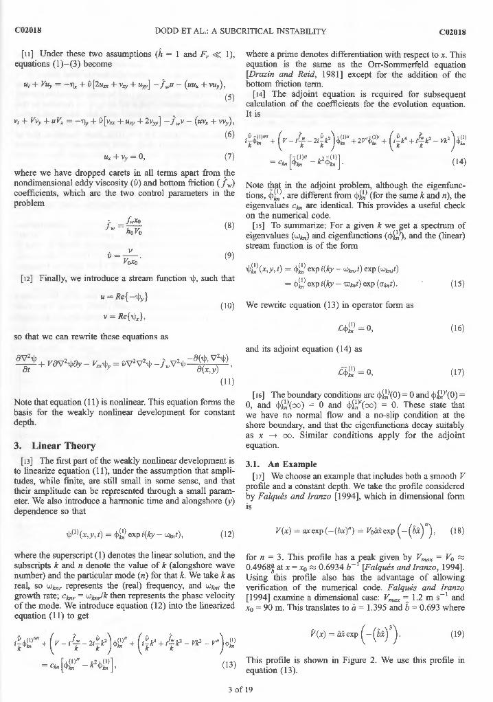
3.1. An Example [ 11] We choose an example that includes both a smooth V

profile and a constant depth. We take the profile considered by Falques and Iranzo [1994], which in dimensional form is

V(x) = a.xexp ( -(bx)") = Voil.X exp ( - (bx) "), ( 18)

for n = 3. This profile has a peak given by V max = Vo ~ 0.4968~ at x = x0 ~ 0.6934 b- [Falques and Iranzo , 19~4]. Using this profile also has the advantage of allowmg verification of the numerical code. Falques and Iranzo [1994] examine a dimensional case: Vmax ~ 1.2 m s- 1 and Xo = 90 m. This translates to a = 1.395 and b = 0.693 where

v(x) = axexp ( -(b.xr). ( 19)

This profile is shown in Figure 2. We use this profile in equation (13).

3 of 19

C02018 DODD ET AL.: A SUBCRJTICAL INSTABILITY C02018

0.8

1.5 2 2.5 3 3.5 4

0.5 :8:)(

0 >

-0.5

-1 0 0.5 1.5 2 2.5 3 3.5 4

-2

0 0.5 1.5 2 2.5 3 3.5 4 x [non-dim.]

Figure 2. Nondimensional V, Vx, and V xx profiles of longshore current profile (equation ( 18)) [Falques and Iranzo, 1994].

[1s] We first solve the inviscid problem C.lw = iJ = 0); see Figure 3. The same growth rate curve is shown in Figure 9 of Falques and Jranzo [ 1994] (in nondimensional units). When compared, results are identical. An interest­ing feature is that the growth rate curve possesses two maxima, which do not correspond to different modes (see Figure 3). A

[1 9] For constant depth, results for fw =f. 0 (bottom friction present) can be obtained from those for .lw = 0 by replacing VJ~c11 by W~c11 = VJ~c11 - ].,. The effect of bottom friction is therefore to reduce growth rates uniformly for all k, with frequencies unaffected. Results for ]IV =f. 0 are therefore obtainable directly from those for ]IV = 0, so we retain ]IV = 0 for the remainder of this section.

3.2. Eddy Viscosity and Viscous Destabilization [20] The introduction of eddy viscosity has a pro­

nounced effect. The gradual increase of viscosity can be seen in Figure 4 (positive growth rates) and Figure 5 (frequencies). It results in the appearance of a separate mode, initially with small growth rates, which for 0.0002 < iJ < 0.0005 yields a distinct instability curve (see Figure 5 for the equivalent dispersion lines). Thereafter, this curve is damped and the "main" curve dominates when iJ =

0.005. [21] As 0 increases, a spectrum of dispersion curves

emerges; see Figure 5. Most of these are decaying (stable) modes, so their growth rates are not apparent in Figure 4. By iJ = 0.04, there is a clear dividing line between two sets of modes (only the first 15 obtained from the numerical solution are shown here). This line separates shear wave

type modes (which possess exponentially decaying asymp­totic behavior as k--> oo, and are true physical modes in that they converge as the number of computational nodes, N -->

oo) from numerical ones (which exhibit neither of these behaviors). (Note that there may be some true solutions with asymptotic oscillatory behavior as k --> oo included in this set, but they are not physically relevant; we do not pursue this here, however; see Appendix B). The shear wave modes all are stable for iJ = 0.04. Note, however, that as iJ changes, the main shear wave dispersion curve remains largely unaffected, whereas the other shear wave curves move noticeably. We refer to these latter modes as viscous modes. Note that we also solved this problem without imposing the boundary condition <P~~'(O) = 0, in order to test the robustness of the solution. Results were qualitatively and quantitatively very close to those presented throughout this paper.

[22] This progression shows the initial destabilization induced by the eddy viscosity. For 0.00001 < iJ < 0.00 I the maximum growth rate increases from about a ;::::::; 0. J 20 for iJ = 0.00001 to a ;::::::; 0.127 for iJ = 0.00 I. Falques et a/. [1994] and Caballeria eta!. [1997] both note this behavior, but for nonconstant v with a maximum around the position of V,wx·

[23] Putrevu eta!. [1998] examine this effect for constant v using the Bowen and Holman [1989] profile. They note that viscosity extends the range of instability and increases

I .'!'.. 13

0.016

0.014

0.012

0.01

0.008

0.006

0.004

0.002 :

~L-----0~.0-1----0~.0-2~

k[m-1]

I .'!'.. t>

X 10-3

1.5

... ·--· ..

.. ·.

0.5

~L_----o~.o-1----o~.oL2~

k [m-1]

Figure 3. (left) Dispersion diagram, and (right) corre­sponding growth rate curves, for equation ( 13) and V profile (equation (19)) for iJ = j w = 0.0. Quantities are shown in dimensional units based on scalings vmax = 1.2 m s- 1 and x0 = 90 m. Note that in the numerical code a value of 0 =

0.000001 is used.

4 of 19

C02018 DODD ET AL.: A SUBCRJTlCAL INSTABILITY C02018

~~ . \

\

0.1 (\ "' ! \

0.15

0.1

"'

0 1 2 0 1 2 k k

Figure 4. Positive growth rates as a function of k (nondimensional quantities) for V profile (equation (19)) for eddy viscosities (] w = 0) (from top left to bottom right): i) = 0.00001, 0.0001, 0.0002, 0.00025, 0.0003, 0.0004, 0.0005, 0.001, 0.005, 0.01, 0.02, 0.04.

the growth rates. Putrevu et al. [1998] find that for I o-4 < v < 10- 1 m2 s- 1

, increased viscosity destabilizes the current, and that this includes the physically relevant interval 10- 3 < v < 10- 1 m2 s - I, which translates into approximately 10- 5 < iJ < 0.001, the upper bound of which is also roughly the value of iJ giving the peak growth rate here; see Figure 4.

[24] In the present model the maximum dimensional growth rate is cr:::::; 0.0017 s- 1

, for v:::::; 0.1 m2 s- 1• That

predicted by Putrevu et al. [1998] is cr :::::; 0.009 s- 1•

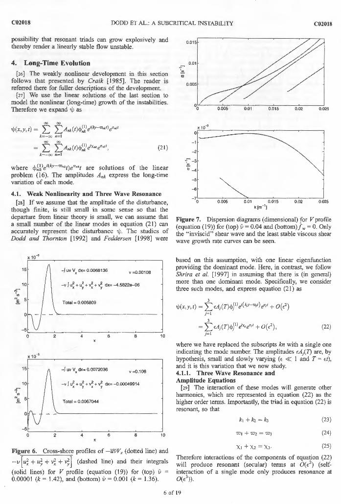
However, for larger v the growth rate continues to increase in the Putrevu et al. [1998] model, so it is not clear if, and if so where, a peak exists for that simplified problem. Nevertheless, the explanation of Putrevu et al. [1998], that phase changes in velocity components induced by the inclusion of eddy viscosity result in energy extraction from the longshore current and therefore further destabilization, seems to apply here too. This can be seen in more detail in Figure 6, in which the two terms on the right of the energy equation,

(20)

are plotted, for iJ = 0.00001 (k = 1.42), and iJ = 0.001 (k = 1.36), each k being the peak of the growth rate curves for that value of iJ. The direct effect of dissipation is very small, even for v = 0.001 (apart from very near to x = 0), but it is always

purely to damp. However, the mixing term is also affected, with a stabilization around its main peak (corresponding to the backshear in V), but a destabilization nearer to the shore. The result is a small overall destabilization in the mixing term. The total effect (mixing plus eddy viscosity) in this figure appears to be a slight stabilization (contrary to Figure 4), but this is due to the normalization used (maxi <P I = I and 1m { <P } = 0 when I<P I = 1 ), which, for different k, results in different velocity magnitudes (for iJ = 0.00001, Um ax = 1.704 m S- l and Vmax = 1.95 m S-

1; for V = 0.001, Umax =

1.632 m s- 1 and Vm ax = 1.919 m s- 1). Normalization with

equal velocities gives us a destabilization, in line with Figure 4. The present study therefore corroborates the findings of Putrevu et al. [ 1998].

[zs] In the next section we develop the weakly nonlinear theory, and apply the theory to a test case. A realistic value for iJ is iJ :::::; 0.001 - 0.01 (corresponding to v :::::; 0.1 - 1 m2 s- 1

) , including the effects of dispersive mixing [Ozkan-Haller and Kirby, 1999]; this implies instability. But it is the stable current that is most interesting, because this provides us with an opportunity to see if finite amplitude destabilization can be observed for a linearly stable flow. Therefore we choose iJ = 0.04 (v = 4.32 m2 s- 1

) . We show the full dispersion diagrams (those including negative growth rates) for this example in Figure 7. Note that in this figure we removed all the numerical modes, and we present dimensional growth rates and frequencies. In the next section we focus on the case iJ = 0.04 and investigate the

1 2 k

1 2 k

0 1 2 k

0 1 2 k

Figure 5. Dispersion diagrams (nondimensional) for V profile (equation (18)) for eddy viscosities (j w = 0) with (from top left to bottom right) : iJ = 0.00001, 0.0001, 0.0002, 0.00025, 0.0003, 0.0004, 0.0005, 0.001, 0.005, 0.01, 0.02, 0.04.

5 of 19

C02018 DODD ET AL.: A SUBCRITICAL INSTABILITY C02018

possibility that resonant triads can grow explosively and thereby render a linearly stable flow unstable.

4. Long-Time Evolution

[ 26] The weakly nonlinear development in this section follows that presented by Craik [ 1985]. The reader is referred there for fuller descriptions of the development.

[ 21] We use the linear solutions of the last section to model the nonlinear (long-time) growth of the instabilities. Therefore we expand 'ljJ as

k=-oo n= 1 00 00

= 2:::: l::=Ank (t)<j>~~)eiXn<e"•*t, (21 ) k=-oo n=l

where <P~Vei(ky-""•*t)e"•*t are solutions of the linear problem (16). The amplitudes Ank express the long-time variation of each mode.

4.1. Weak Nonlinearity and Three Wave Resonance [ 28] If we assume that the amplitude of the disturbance,

though finite, is still small in some sense so that the departure from linear theory is small, we can assume that a small number of the linear modes in equation (21) can accurately represent the disturbance 'ljJ. The studies of Dodd and Thornton [1992] and Feddersen [1998] were

-1 uv Vx dx= 0.0068136 v =0.00108

-v I u2 + u2 + ~ + ~ dx= -4.5822e-06 X y X y

Total= 0.006809

4 6 8 10 X

-I uv Vx dx= 0.0072036 v =0.108

-vI u2 + u2 + ~ + ~ dx= -0.00049914 X y X y

7 UJ

"' .s Total = 0.0067044

-5L_ ____ ~-------L------~------~----~ 0 2 4 6 8 10

X

Figure 6. Cross-shore profiles of -uvVx (dotted line) and

-v [u; + u; + v; + ~ J (dashed line) and their integrals

(solid lines) for V profile (equation (19)) for (top) 0 0.00001 (k = 1.42), and (bottom) 0 = 0.001 (k = 1.36).

-1

-2

~~ -3

t:> -4 ··,

-5

-6

-? o'----...,o,..,.o'-os=----~o ..... o1 _____ o=-.o'-1,-5 -----=-o.,..,.o2,_---o,--J.o2s k[m- 1]

Figure 7. Dispersion diagrams (dimensional) for V profile (equation (19)) for (top) 0 = 0.04 and (bottom)] w = 0. Only the " inviscid" shear wave and the least stable viscous shear wave growth rate curves can be seen.

based on this assumption, with one linear eigenfunction providing the dominant mode. Here, in contrast, we follow Shrira et al. [ 1997] in assuming that there is (in general) more than one dominant mode. Specifically, we consider three such modes, and express equation (21) as

3

'\)J(x,y, t) = 2:::: EAj(T)<J>j')ei(k;y-w;t)e"JI + O(t:2) j=l

3

= l::= EAj(T)<J>)')eiX;e";t + 0(t:2),

j= l (22)

where we have replaced the subscripts kn with a single one indicating the mode number. The amplitudes €Aj(1) are, by hypothesis, small and slowly varying ( E « 1 and T = Et), and it is this variation that we now study. 4.1.1. Three Wave Resonance and Amplitude Equations

[ 29] The interaction of these modes will generate other harmonics, which are represented in equation (22) as the higher order terms. Importantly, the triad in equation (22) is resonant, so that

X1 +xz = X3·

(23)

(24)

(25)

Therefore interactions of the components of equation (22) will produce resonant (secular) terms at 0(E2

) (self­interaction of a single mode only produces resonance at 0(E3

)).

6 of 19

C02018 DODD ET AL.: A SUBCRITICAL INSTABILITY C02018

0.8

13 0.6

0.4

Triad C

k k

Figure 8. Dispersion diagrams (nondi~ensional) for V profile (equation (18)) for 0 = 0.04 and f w = 0. Solid line arrows are the triad vectors: [kt, w 1] , [k2 , w2] and [k3, w 3]

of the resonant triads; (a = 1.395, b = 0.693, n = 321 ,jw = 0). Only the first 30 eigenmodes, in order of increasing decay rate, are plotted. Note that for Triad F a different scale has been used to illustrate the whole triad.

[3o] The remainder of this standard development is pre­sented in Appendix A 1. The result is a set of three nonlinear amplitude equations,

(26)

(27)

(28)

where I-Lt ,2,3 are complex constants (see Appendix Al), a 1,2,3 = A1,2,3e0

' ·2

·'' , and an asterisk denotes a complex conjugate. 4.1.2. Analytical Results

[3t] The system of equations (26)- (28) admits explosive solutions under certain initial conditions and for certain values of Gj and I-Lj · Unfortunately, no necessary and sufficient conditions are known to the authors (see Craik [ 1985] for a discussion of some special cases). Wang [1972] derives sufficient conditions for the non-existence of explo­sive solutions for general values of Gj and I-Lj· In our case we have Gj < 0 for allj, so a stable node exists at a 1 = a2 = a3 =

0. Therefore, near enough to this node, we have asymptot­ically exponentially decaying solutions (the linear decay). In fact, it can be shown in a similar manner to Wang [1972] that any solution satisfying the condition

(29)

tends to the origin as t --+ oo, where G = miniGjl forj = 1, 2, 3, as does any solution such that

(30)

where j.L = max ii-Ljl forj = 1, 2, 3. While these conditions are only sufficient (i.e. , not satisfying them does not imply instability), it seems reasonable to suppose that their relative size may give an indication as to the likelihood of finding explosive solutions for given values of I-Lj and Gj. Note, also, that different normalizations of ¢Jl l lead to different values for I-Lj (although the system_ is invariant to the normalization of the adjoint functions ¢jll). Results given by different normalizations are directly transformable between each other; see Appendix A.

4.2. Resonance in Our Example [32] We can find resonant triads in the dispersion diagram

for 0 = 0.04, either considering modes lying on only one dispersion curve, or on different ones, as well as taking the same mode twice. A number of such triads are shown in Figure 8. In Triad A we take one mode twice. Triad B includes the fastest growing (here slowest decaying) mode. This mode has a dimensional growth rate of - 6.1 X 1 o-5 s- 1

. Triad cis representative of the family of modes that lie on the main dispersion line, of which A and Bare special cases. Triads D, E, and F include viscous modes. Interestingly, one such mode (in Triad D) is situated at the point at which two modes cross, so, in theory, we could take either in our triad. However, the growth (decay) rates are very different: - 8.2 X 10- 5

S- l for the mode on the main dispersion curve; - 6.6 x 10- 3 s- 1 for the viscous mode. Note also that in both Triads D and F, one mode is the same as that occurring in Triad A (k = 0.72). In Table 1 the values of k, w, and G associated with these triads are given, along with the analytical estimates B 1 and 8 2 and an indication (~w) of the departure from exact resonance of the values shown.

[33] On the basis ofthe estimates (equations (29) and (30)) (see Table 1), it appears that Triad B, including the FGM, would be the best candidate for investigation. We begin here. 4.2.1. Triad B

[34] Numerous numerical experiments were tried. All these experiments ultimately resulted in an " explosion" (i .e., unbounded growth in a finite time), if a large enough initial amplitude was defined. Initially, the procedure was to fix one initial mode amplitude at zero, assign a second some finite value, and vary the third until an explosion was encountered, thus establishing a threshold. Then the second amplitude was incremented and the process repeated, which resulted in three sets of initial amplitudes, corresponding to the three different modes. Numerical integration was carried out using a Gear method, which is particularly suited to

7 of 19

C02018 DODD ET AL.: A SUBCRlTICAL INSTABILITY

Table 1. Table Showing Nondimensional Resonant Wave Numbers (k;) and Frequencies (m;), as Well as (Dimensional) Decay Rates (a;), Values of 1-J.;, Nearness to Exact Resonance (6-m), and Two Analytical Estimates of Amplitudes Below Which Explosive Growth Cannot Occur (8 1 and 8 2) for the Resonant Triads Shown in Figure ga

k tv· r:r · ll. tv 81 Bz

A 0.720 0.322 -0.0090 0.219 - 0.926i 0.720 0.322 - 0.0090 0.2 19 - 0.926i - 1.43 X 10- 4 0.028 0.028 1.440 0.645 -0.0547 - 0.514- 0.216i

B 0.550 0.275 -0.0 178 0.094 - 1.649i 0.910 0.387 - 0.0046 0.320 - 0.403i 4.89 X 10- 3 0.013 0.008 1.460 0.657 - 0.0588 - 0.500 - 0.169i

c 0.300 0.202 -0.0322 0. 704 - 2.456i 1.450 0.651 - 0.0567 0.370 + 0.444i 5.89 X 10- 3 0.067 0.038 1.750 0.847 - 0.1373 - 0.355 + 0.376i

D 0.720 0.322 -0.0090 -0.042 - 0.297i 0.910 0.387 - 0.0046 0.018 - 0.133i 5.30 X 10- 3 0.012 0.046 1.630 0.705 - 1.1210 - 0.387 + 1.443i

E 0.360 0.222 -0.0289 - 0.734 - l.IIOi 0.550 0.166 - 0.4152 0.310 + 0.168i 9.40 X 10- 4 0.024 0.011 0.910 0.387 -0.0047 - 0.097 - 0.077i

F 0.720 0.322 - 0.0090 1.340 + 0.167i 2.250 1.270 - 0.3423 - 0.050 + 0.349i 3.90 X 10- 3 0.044 0.020 2.970 1.588 - 1.5796 - 0.251 + 0.745i

G 0.930 0.476 - 0.0015 0.725 - 9.744i 0.930 0.476 - 0.0015 0.725 - 9.744i 3.2 X 10- 4 0.016 0.018 1.860 0.952 - 0.00079 - 0.924 + 0.359i

•see section 4.2. Note that normalization of eigenfunctions is the same for all triads: max ie!> I = I. The final triad (G) is depicted in Figure 19.

dealing with stiff problems [Press et a!., 1992]. They were subsequently verified using a Runge-Kutta solver. As mentioned, explosive growth was always observed if the variable amplitude was increased enough.

2

"' 0

C02018

[35] Of particular interest is the smallest amplitude nec­essary for explosive instability. All combinations of modes showed a minimum amplitude similar in size in each case, but noticeably smaller when the two non-zero amplitudes included component a2, the least stable mode. This seems physically reasonable since the linear decay associated with a2 is comparatively small. We do not present here all the results of the numerical experiments, as they were qualita­tively similar to each other. Instead we focus below on the amplitude necessary to achieve this explosion, and on the dimensional time taken for this to occur.

-2 -20~---------------'

[36] In Figure 9 we show an example of one such critical amplitude being established in the numerical experiments. Of particular note here are the top two panels, which show such a threshold being encountered for one set of initial conditions. The top left panel shows a stable set of initial conditions (the linear decay can be seen in the plot of the log amplitudes immediately below). The top right panel shows the explosion resulting when the initial amplitude lla(O)II is increased a little further; the explosion can clearly be seen, and the growth is evidently faster than exponential. Finally, note also that initial conditions like some of those here (one zero, one finite, and one finite but small ampli­tude) approach a stable node of the system (if two initial amplitudes are zero, then they will remain so and the third will decay exponentially; see Appendix A). This seems to be what we find.

[37] The time that it takes for an explosion to occur for a given initial condition (texp) is also significant. Changes in texp resulting from further (small) increases in lla(O)II can also be seen in Figure 9. The explosion is evident (top right panel) and occurs after 506 nondimensional time units

2

"' 0 .1. -----..;;>

-2

2

"' 0 .L::I --2~----~------~

2.--,.----------,

"'0~

-2L_~L---------~ 0 200 400 600

t (non-dim)

10.------------.-,

200 400 600 t (non-dim)

Figure 9. Amplitudes and log amplitudes of modes for Triad B for four different initial amplitudes for (top row) a 1(0) = 0.02, a2(0) = 0.147; (second row) a 1(0) = 0.02, aiO) = 0.148; (third row) a 1(0) = 0.02, a2(0) = 0.149; (bottom row) a 1(0) = 0.02, a2(0) = 0.160.

8 of 19

C02018 DODD ET AL.: A SUBCRITICAL INSTABILITY C02018

11

10

9

8

7

~ 6 ~ 0 ~

a. 1ij 5 -

4

3

2

OL-~------L-----~----~------~----~

0.17 0.18 0.19 0.2 0.21 0.22 lla(O)I I

Figure 10. Times until an explosion Ctexp) as a function of initial triad "energy" (Triad B).

(ndtu). Also shown are similar explosions for very small further increases in initial amplitudes of less than 1% and about 6%. Note that just a 1% increase in "amplitude" of the triad Clla(O)II) gives a reduction in explosion time of 50%.

[38] This is further illustrated in Figure 10. Here, how­ever, we plot the dimensional time it takes for an explosion to occur against the initial amplitudes. The dramatic de­crease in time taken for just a very small increase is readily apparent. The effect of further increases in initial amplitudes is less pronounced. Note that a 13% increase in initial amplitudes from critical values gives an explosion time of about 2.5 hours, and a 25% increase results in 2.0 hours. It is worth noting that Ozkan-Haller and Kirby [1999] report that their numerical simulations (of the SUPERDUCK data sets) reach finite amplitude within about 30 min to 1 hour, depending largely on the eddy viscosity coefficient (albeit for a linearly unstable flow). Approximately similar results are reported by Slinn et al. [1998].

[39] To get a better idea of the overall picture, we also run numerous simulations with random initial amplitudes. The procedure followed was to initialize each real and imaginary part of each of the three complex amplitudes such that

Re{ aj(O)} = FB2r

Im{ aj(O)} = FB2r, (3 1)

for j = 1, 2, 3, where each r is an independent random number uniformly distributed between ±1, B2 is the analytical stability bound (equation (30)), and (in this case) F = 10. Thus we have random phases and random initial amplitudes

distinctly above the sufficient stability bound B2 . The results of 10,000 such simulations are shown in Figure 11 . Note that all simulations were tenninated after 1000 ndtu ( ~2 1 hours) if an explosion had not already been encountered, implying that the initial conditions resulted in stability. These non­explosive simulations are indicated at the top of the figure . The explosive simulations can be seen clearly, and are mostly clustered between l and 6 hours. The stable simulations all appear at the top of the figures (at 1000 ndtu).

[4o] The importance of the initial amplitude of the a2 mode can be further seen when each individual amplitude is plotted in the same way. There is an apparent threshold of la2(0) I ~ 0.05 that is required for explosive growth. The a2 mode possesses the smallest decay rate, so its presence for explosive growth to occur seems intuitively reasonable. There is apparently no such threshold for a 1• The mode a3

seems (somewhat counterintuitively) also to possess a threshold. However, we know from our earlier experiments with a(O) = (0.02, 0.148, 0.0) that no such threshold exists. In fact, taking larger initial amplitudes in a 1 or a2 allows a3(0) to be arbitrarily small. The same is also true for a 1 (0).

~ ~ 0 E.

a. X w

~ ~ 0 E.

lt w -

20

15

10

5

0 0

0.1 0.2 lla(O)II

0

00

t 0.1 0.2

la2(0)I

15

0 10

20

15

10

5

0.3 0 0

0

. 0 0

0.1 0.2 la

1(0)1

0

&

01 0.1 0.2

la3(0)I

0.3

0.3

Figure 11. Plot of the dependence of teAP (hours) on initial amplitudes for 20,000 random simulations based on equation (31) for F = 10 for Triad B. Circles indicate the value of texp for a given initial amplitude for a simulation run until an explosion is encountered, or until 1000 ndtu (~21 hours). (top left) Total amplitude lla(O) II also shown is the analytical threshold B2 (dashed line), and the "manu­ally" established threshold amplitude lla(O) II = 0.168 (dotted line); (top right) la 1(0) I also shown is the manually established threshold amplitude component a 1(0) = 0.02 (dotted line); (bottom left) la2(0)1 also shown is the manually established threshold amplitude component a 1(0) = 0.148 (dotted line); (bottom right) la3(0)1.

9 of 19

C02018 DODD ET AL.: A SUBCRJTICAL INSTABILITY C02018

Table 2. Triad A: Nondimensional Initial Amplitudes Necessary for Explosive Growth to Occur in the System of Equations (32) and (33) for V Profile (Equation (19)) for 0 = 0.04a

a 1{0) OJ(O) 11 5(0) 11 a 1(0) OJ(O} 11 5{0} 11

0.0010 0.33150 0.3325 0.11 32 0.05000 0.1632 0.0050 0.23600 0.2410 0. 1146 0.04000 0.1546 0.0100 0.19500 0.2050 0.1137 0.03000 0.1437 0.0200 0.15480 0.1748 0.1112 0.02000 0.1312 0.0300 0.13240 0.1624 0.1075 0.01000 0.1175 0.0350 0.12430 0.1593 0.1071 0.00900 0.1161 0.0400 0.11760 0.1576 0.1067 0.00800 0.1147 0.0450 0.11180 0.1568 0.1062 0.00700 0.1132 0.0500 0.10670 0.1567 0.1053 0.00500 0.1103 0.0550 0.10230 0.1573 0.1034 0.00100 0.1044 0.0600 0.09827 0.1583 0.1030 0.00010 0.1031 0.0650 0.09461 0.1596 0.1029 0.00000 0.1029 0.0700 0.09120 0.1612 0.0750 0.08794 0.1629 0.0800 0.08474 0.1647 0.0850 0.08151 0.1665 0.0900 O.D7813 0.1681 0.1000 O.D7027 0.1703 0.1003 0.07000 0.1703 0.1088 0.06000 0.1688

•Figures are correct to four significant figures.

Thus it is the total amplitude (here 115(0) 11) that is crucial to the subsequent development of subcritical instabilities, which can also be seen if a larger value ofF in equation (31) is taken.

[41 ] However, these apparent thresholds are significant. This is because in reality (as we shall see) a value of 115(0)11 = 0.168 (achieved right at the stability threshold and representing a small such value; see Figures 9 and 11) still represents a substantial "push" to the system, and means that for practical purposes, there probably is a

0.3

0.25 UNSTABLE

0

0.2 0

-"' "' ~ a:

0.15 0

0 0

0 0

0 0.1 0 0 0

0 0 0

0 0

0

0

0.05 STABLE 0

0

0

0

# 0.02 0.04 0.08 0.1 0.12

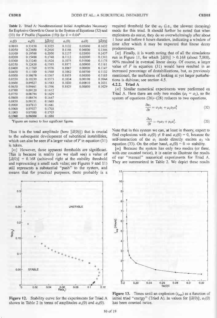
Figure 12. Stability curve for the experiments for Triad A shown in Table 2 in terms of amplitudes a 1(0) and a 3(0).

required threshold for the a2 (i.e., the slowest decaying) mode for this triad. It should further be noted that when explosions do occur, they do so overwhelmingly after about l hour and before 6 hours duration, indicating a window of time after which it may be expected that linear decay predominates.

[ 42] Finally, it is worth noting that of all the simulations run in Figure 11, for which 115(0)11 > 0.168 (about 7,000), 90% resulted in eventual linear decay. Of course, a larger value of F in equation (31) would have resulted in an increased percentage of destabilizations, but, as previously mentioned, the usefulness of looking at yet larger perturba­tions is dubious; see section 4.5. 4.2.2. Triad A

[43] Similar numerical experiments were performed on Triad A. Here there are only two modes (a 1 = a2), so the system of equations (26)- (28) reduces to two equations,

(32)

(33)

Note that in this system we can, at least in theory, expect to find explosions with a 1(0) :1 0 and a 3(0) = 0, because the self-interaction of the a 1 mode directly excites a3 via equation (33). On the other hand, a 1 (0) = 0 "* stability.

[44] Because the system has only two modes (or three, with one counted twice), it is easier to illustrate the results of our "manual" numerical experiments for Triad A. They are summarized in Table 2. We depict these results

11.----.-----.-----.-----.-----,----,-,

10

9

8

7

!:'! 6 :::> 0

6 ~ 5 "' ~

4

3

2

8.2 0.22 0.24 0.26 0.28 0.3 0.32 lla(O)II

Figure 13. Times until an explosion Ctexp) as a function of initial triad "energy" (Triad A). In values for 11 5(0)11 , a 1(0) has been counted twice.

10 of 19

C02018 DODD ET AL.: A SUBCRITICAL INSTABILITY C02018

20

15 15

~ :::l 0 E. 10

§~ 10 0~ c.

X ~ 0 -"'

' 5 5

0 0 0.05 0.1 0.15

0 0 0.05 0.1 0.15

lla(O)II la1(0)1

20

15

~ :::l 0 E. 10

0CXJ 00

~ 0 @ -"'

I 5

0 0 0.05 0.1 0.15

la3(0)1

Figure 14. Plot of the dependence of l exp (hours) on initial amplitudes for 50,000 random simulations based on equation (31) for F = 2 for Triad A. Circles indicate the value of t exp for a given initial amplitude for a simulation run until an explosion is encountered, or until 1000 ndtu (;:::;21 hours) . (top left) Total amplitude ll a(O) II ; also shown is the analytical threshold B2 (dashed line), and the manually established threshold amplitude ll a(O) II = 0.103 (dotted line) ; (top right) la 1(0) I also shown is the ' manually ' established threshold amplitude component a 1(0) = 0.103 (dotted line); (bottom left) la3(0)I (bottom right) total amplitude ll a(O) II for F = 10; also shown is the analytical threshold B2 (dashed line), and the manually established threshold amplitude ll a(O) II = 0.103 (dotted line). Note that these values of ll a(O) II imply that a1(0) is counted just once.

graphically in a corresponding stability diagram; see Figure 12. Once more, explosions were always obtained with a big enough initial amplitude. It is interesting to note that the smallest critical amplitudes were encountered for a3 = 0, which, again, seems reasonable because this mode possesses a much larger linear decay rate than a 1• Note, however, the existence of another local critical amplitude minimum at about a 1(0) = 0.05 and a3(0) = 0.1067.

[ 45] In Figure 13 we again show the variation in l exp

starting from critical conditions (a 1 (0) = 0.1 03 , a3(0) = 0), gradually increasing the amplitude a 1 (0). A similar picture to that seen in Figure 1 0 is observed.

[46] Once again , we show a more comprehensive set of (50,000) numerical experiments, in Figure 14. Again, each symbol shows l exp for that ll a(O) II and, once more, an apparent threshold emerges, this time for ah significantly lower than a1 = 0.1 03 . As before (Triad B), this is not strictly a threshold (explosions for arbitrarily small, finite

values for a 1 can be found), but in practical terms it probably does constitute a threshold for subcritical insta­bilities. Once again, explosions occur overwhelmingly between 1 and 6 hours. If we consider again the ratios of explosive to stable simulations, we find that for runs such that ll a(O) II > 0.103 (about 12,000 for F = 2 for these calculations), 91 % resulted in eventual linear decay.

[ 47] Finally, to illustrate the effect of taking a larger value for F, we show in the fmal panel of Figure 14 the Cll a(O) II , lexp) plot for another set of simulations for which F = 10. It can immediately be seen that the threshold we established by earlier experiments Cll a(O) II;:::; 0.103, taking a1 just once) is real. In contrast, there are no apparent thresholds for a 1 or a3 (not shown). For F = 10, 95% of all simulations for which ll a(O) II > 0.103 are explosive.

4.3. Triads C-F [48] Similar numerical experiments were performed on

Triads C-F. Only Triad D exhibited explosive instabilities despite (in the cases of Triads E and F) values ofF = 50 being used. The results for Triad D were qualitatively similar to those for Triad B, with a threshold of lla(O) II ;:::; 0.3. Again, the greatest individual threshold dependence is on the slowest decaying mode (in this case, mode 2).

[49] The stability thresholds established for Triads A and B are nondimensional at this point. It is necessary to convert them into dimensional predictions to see if they are phys­ically relevant estimates. Before doing this, we first see if the amplitude equations for non-exact resonance exhibit similar behavior.

4.4. Approximate Resonance [so] Recall that in Table 1 we showed values D.m, which

provide a measure of the degree to which the resonant triads are not exact. It is important to consider the effect of non­exact resonance because in the field, this type of resonance is likely to be found, rather than exact resonance.

[s1] For non-exact (temporal) resonance,

(34)

(35)

so that

X i + X2 = X3 - D:rot , (36)

X3 -Xi = X2 + D:rot , (37)

X3 - X2 =Xi + D:rot. (38)

In these circumstances the amplitude equations (26)- (28) become

(39)

(40)

( 41 )

II of 19

C02018 DODD ET AL.: A SUBCRJTICAL INSTABILITY C02018

Table 3. Table Comparing Critical Amplitudes for Most Unstable Initial Conditions of Triad A (Table 2) for Exact and Approximate Resonance Equations

Equations (26) - (28)

Triad .6.1:0 a1(0) az(O) GJ(O)

A - 1.43 X 10 4 0. 1030 0.0000 0.0 A - 1.43 X 10 4 0.0900 0.0900 0.0782 A - 1.43 X 10 4 0.0600 0.0600 0.0983 A - 1.43 X 10 4 0.0 100 0.0100 0.1950 A - 1.43 X 10- 4 0.0010 0.0010 0.3315

[52] In order to see if this non-exact resonance has a substantial effect on the critical amplitudes we performed further numerical experiments, in which the deviation from exact resonance noted in Table 1 is used in the system of equations (39) - (41 ). In Table 3, some results for Triad A are shown. It can be seen that there is little difference between exact and non-exact results in terms of critical boundaries. Progressively larger values of ~w lead to larger required values of lla(O) II for explosions to be observed (not shown). However, the values are not significantly larger than those required for exact resonance. This was a general feature of the experiments we performed. The result implies that it is sufficient to consider conditions close to exact resonance in order to get realistic, physical predictions.

4.5. Dimensional Amplitudes [53] For the predictions of sections 4.2. 1 and 4.2.2 to be

physically meaningful , we need to convert them to dimen­sional predictions and relate them to the longshore current. In Figure 15 we show the dimensional values of lui, lvl and the associated free surface elevations for explosive conditions for Triad 8 (a(O) = (0.02, 0.148, 0)) shown in Figure 9. In Figure 16 we do the same for Triad A (a(O) = (0.103, 0.103, 0)).

[54] In both cases the free surface elevations shown are reconstructed from the y momentum equation,

(

W . V 2 ]w) . V " . V' , "' = - - V + 2t - k + -. V - 1 - V + I- U + VU . 'I k k k k k '>

(42)

and are very small, as expected. (Note that there is some loss of significant figures in calculation of 11 in some areas of the profile for both triads .)

[55] The perturbations shown in Figures 15 and 16 are substantial in terms of a proportion of the maximum long­shore current (1.2 m s- 1

). The total variation (i.e., maximum positive to negative velocity) in the Triad 8 case is about 0.04 Vm<L< for VJ and 0.02 Vmax for u 1, and about 0.35 Vmax for v2 and 0.27 Vm<L< for u2 , where u 1 is the velocity associated with the a 1 mode, etc. For the Triad A example (Figure 16), these figures are 0.23 Vmax for v 1 and 0.15 Vmax for u 1• To give an idea ofthe size of these perturbations, we show in Figure 17 a vector plot of the perturbation for the Triad A example above, superimposed on the background longshore current. It can be seen that these perturbations, though reasonably large, do not dwarf the mean current, and are perhaps not inconsistent with naturally occurring perturbations.

5. Inclusion of Bottom Friction

[56] The analysis of the preceding section seems to indicate that this kind of explosive growth might be possible

A~~roximate Eguations (39)- ( 41)

lla(O) II a 1(0) az(O) a3(0) lla(O) II 0.2060 0.103 0.0000 0.0 0.2058 0.2582 0.0900 0.0900 0.0782 0.2581 0.2 182 0.0600 0.0600 0.0983 0.2182 0.2150 0.0100 0.0 100 0.1950 0.2150 0.3335 0.0010 0.0010 0.3315 0.3335

in realistic flows . However, so far we have examined flows without bottom friction. This was because the linear stabil­ity results with bottom friction follow straightforwardly from a simple transformation. However, in realistic flows, bottom friction will also play a substantial role in suppress­ing (linear) instabilities. Therefore, in such a realistic flow, which is linearly stable but close to instability (and thus a candidate for possible explosive growth; recall that we apparently need at least one mode of a triad with a small decay rate), the eddy viscosity will be significantly smaller than 0 = 0.04, and so the bottom friction will contribute. Therefore the linear dispersion curves are likely to be significantly different from those for i) = 0.04 and ]"' = 0.0 (Figure 7).

[57] In Figure 18 we show a dispersion diagram for i)= 0.001 (v = 0.108 m2 s- 1

) and]w = 0.13. This value ofv is more representative of that usually taken in the surf zone [see Ozkan-Haller and Kirby, 1999]. The dimensional value f.v will depend on the constant depth chosen, but an order of

~~ 0.01K ----.:_______.................... .... . . ... . .. l ¥, -o o~L__---""--~o<::::..-..__ __ .. _ .............. _ .... _ ... _ ... _ .. _ .. _ ......... _·_· _· _· _· _·_J

-i_:~b>=?==' ',,, ,,, ' ·l X 10"3

0 2 4 6 8 10 x lNon-Diml

Figure 15. Dimensional lui, lvl, and 1111 envelope profiles for explosive initial conditions for Triad 8: a(O) = (0.02, 0.148, 0) ; (top three plots) a1(0); (bottom three plots) a2(0). These conditions lead to explosive growth of system of equations .(26)- (28) for V profile (equation ( 19)) with i) = 0.04 and fw = 0.

12 of 19

C02018 DODD ET AL.: A SUBCRITI CAL INSTABILITY C02018

0.05 I "' .s ,.::::::::::::: ': •: I • I

~ +I

6 8 10

:::::: :::::: ::: :::: :::111 0 I 0 0

6 8 10

···::=====::::::::::::::::::: :""'''''''

.-·

0 2 4 6 8 10 x [Non-Dim]

Figure 16. Dimensional lui, lvl, and 1111 envelope profiles for explosive initial conditions for Triad A: a(O) = (0.1 03, 0.0, 0). These conditions lead to explosive growth of the system of equations (26)- (28) for V profile (equation (19)) with v = 0.04 and Jw = 0.

1500~~~~~m~m;~mn~mn~ma~JJII~~~· .. ~ ... ~ ... :-.~~--,---~---r--l 4PIIJI!Iiiliiiillillilillllliiitttmm •• •.... . .. •. •. • . . •• , . !UUUIIIUUIIilllillhhliilttttnm ....... ......... __ . _. _

;-Ulli!llildlldilihhlhmli1mm ................... . .. . . ;-WIUUMUI!dlihhl\hhltnmmm. ................ . _.

diti\U&Mdllllltulhhmmnmm. ..... ... ... .

-= Md:GMGII!d!ti\\\ltil(((\h(\lhthh1Tt1muo ••... ....

JiJi!i\l!i\(i\(1\\\lliil(\\\l\\(ihjjjjjjtTlTf'tutooo oo oo

a::Gi!GR\1\IIM\Utuhil\hihllilliilitmrr••,. ,.. . . . . . • • • . . . • . .

a&dildbllllitilld\iiihlhiliiihlliiJitfftttrooo•· .. -. .... ... ••.

:§:1000~====== ................... ... -L &llbfiilJIJII/jjjjliJjiJlJJJij/iiifTttrnn ......... . Q) 0 c

"' 1ii '6 ~ 0

.r:. "' Cl c 0 <(

IUJLhilllllllllllilllhllntmr,,,,,,,,.

4ffib/iiliilihii/IJIIIIIIIIiilittm•••••••

llillilliiiillllllliiilliiitmm ..... ...... .. . . . ... .

!bll!IUIII!lhliihlllliilttrnm.. ..... ......... . ... . .. .. .

UUI!IUI!dilhllhiihlilimtmm ............. . . _.

1-iWUII\IiildhliUIIlliimllmmm. ..................... .

500 ----=aa:uuaammmmmnummmrnm,. .......... . tUIUUidllddLUIU\Itiiiltlnmrnm ...... ... .

Hdililitiiilii\ll\\\1((\((\ll\iilhtiilltirntm., .. , ,,,

iifilil\iitililiil\\lhlilliliillliihiflfTTttuttoo oo •·• ,, , , 0 0 , , 0 o o ,

UffiGIIIIiliiliiiilihiliillhillitttmr,,,,,,, •. . . . . . . . . • • • • • •

DIJUibilliililiiliilililhillhffiHrmr, ........... ... ... . . . •

lbblliJjjj)jjjjjjjiJijjJhhhliliitrmm............. • • • • . . • •

4ffibHj)ji)jjjjjiJjjj}jjlhjj/lli#ftmtmooo • ... , , , , 0 , , , , , ,

bLJjjjjjjjii)IJijjj)ihhilifftmm,, ,,,.

0 0 50 1 00 1 50 200 250 300 350 400 450

Cross-shore distance [m]

Figure 17. Vector plot of critical amplitude perturbation for Triad A (a(O) = (0.1 03, 0, 0)) superimposed on the mean current for V profile (equation (18)). The alongshore range is two wavelengths of mode a 1•

' .!!1. 13

x10-3

" -4

-5

-6

-?~----~------~------~----~--~~~

0 0.005 0.01 0.015 0.02 0.025 k(m- 1]

Figure 18. Dispersion diagrams (dimensional) for V profile (equation (19)) for v = 0.001 and Jw = 0.13. The incomplete dispersion lines result there because the associated decay rate (at k ~ 2.3) becomes so large that it no longer constitutes one of the first 30 modes; in reality, it does not suddenly cease at this value.

magnitude estimate can be obtained for h0 = 2 m, which gives f w = 0.0035 m s- 1

• This corresponds to a friction coefficient in a quadratic drag law of cd ~ 0.01 (weak current approximation) or cd ~ 0.003 (strong current ap­proximation), using an orbital velocity of 0.5 m s- 1 and a longshore current of 1.2 m s - I . These values are consistent with those used in nearshore circulation modeling. This case has been chosen to create similar conditions to those for v = 0.04 and Jw = 0.0 (i.e. , subcritical flow near to linear instability); obviously, numerous other possibilities exist for varying v and Jw-

[ss] The smaller eddy viscosity results in a range of smaller decay rates in general (compare Figure 7). Note the richer array of dispersion lines than for v = 0.04 and Jw = 0.0. This seems somewhat counterintuitive because viscosity introduces viscous modes, but it may be that more dispersion lines are present but with decay rates so large (because of increased viscosity) that they no longer appear as one of the 30 least stable modes. This can be seen to happen in Figure 18 (see caption), but we do not pursue this point.

[s9] Once again, numerous candidate triads can be found. We choose one such triad, referred to here as Triad G (see Table 1 ). This triad is illustrated in Figure 19.

[6o] In much the same way as for Triad A, we can manually establish a threshold between stability and insta­bility. We show this in Figure 20. It can be seen that this explosion takes place at 94 ndtu, or 1.96 hours. This is put more into context when we show values for t exp resulting

13 of 19

C02018 DODD ET AL.: A SUBCRlTICAL INSTABILITY C02018

2

TriadG 1.8

1.6

1.4

1.2

13 1

0.8

0.6

0.4

0.2

0.5 k

/

.. ...

1.5 2

/ /

2.5

Figure 19. Dispersion diagram (nondimensional) for V profile (equation (19)) for 0 = 0.001 andj 11 • = 0.13 showing Triad G. The triad is indicated by the arrows.

0.1,----------,

0.05

-0.05

-0.1 L__-~--~-__J

0.1 ,--....,--------,

0.05

-0.05

-0.1 L--'--~------' 0 200 400 600

t (non-dim)

0

-2

- 1 oL---2~00,----4~0.,...0 ---'600

t (non-dim)

Figure 20. Amplitudes and log amplitudes of modes for Triad G at the explosive threshold il(O) = (0.0624, 0.0624, 0) for (top) (a 1(0) = 0.0624, a2(0) = 0.0624, a 3(0) = 0) and (bottom) (a 1(0) = 0.06241 , az(O) = 0.0624 1, a3(0) = 0).

from further small increases in the initial amplitude. We do this in Table 4, in which we take the value identified in Figure 20 (a 1 = 0.06241) as the critical amplitude ac, and refer to increases in proportions of ac,

factor x ac

It can be seen that a 9% increase in a 1(0) approx imately halves fexp· A doubling of the initial amplitude reduces fexp

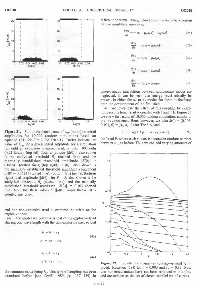
to just 9 min. Clearly, these times are significantly shorter than those observed so far, and this can be seen too in Figure 21, where we show the results of random simulations for F = 2. Note that the final panel in this figure is for a further set of simulations for F = 5 (which again indicate that there is no actual threshold for a3 ),

which appears to show several simulations violating the stability bound. However, note that in this figure the a1

mode is only counted once. Counting it twice reveals no such violation.

[61] It seems therefore that this triad is significantly more "explosive" than either A or B . However, this is not apparently due to the values of v and f.v as such, because Triad D exhibits similar behavior (not shown). More significant are the linear decay rates for Triads D and G. Triad D possesses two very slowly decaying modes (1 and 2) equivalent to those same modes in Triads A and B, respec­tively. All modes in Triad G have small decay rates. It is this that appears to dictate how explosive a triad is. For reasons already discussed, it is likely that considering both eddy viscosity and bottom friction as stabilizing mechanisms will favor such modes (and therefore such triads). If, for instance, we increase 0 in Figure 18 to 0 = 0.005, we note a significant decay in all growth rates except the main inviscid mode; see Figure 22.

6. Coupling of Triads

[62] So far we have seen that explosive triads can exist in physically plausible alongshore flows . The addition of viscosity (and bottom friction) results in a rich array of dispersion curves that can potentially allow many resonant triads to exist. Unlike the example discussed by Shrira eta/. [ 1997] (that of Bowen and Holman [ 1989]), these modes are all decaying for large enough dissipation . It has also been seen that some of the triads are explosive and others are not. Therefore the possibility exists for coupling between triads. In thi s section we investigate the effect of coupling between two triads. It is not difficult to find triads sharing common modes (see Triads A, B, and D; also Triads A and F). In particular, we consider the coupling between one explosive

Table 4. Table of lexp for Different Initial Amplitudes for Triad G"

ac factor Lex n ndtu l ex , hours

0.06241 1.0 94 1.96 0.063 1.01 49 1.02 0.07 1.12 23 0.48 0.08 1.28 15 0.31 0.10 1.60 10 0.21 0.12482 2.0 7 0.15 (~9 min)

"The va lue factor represents the factor by which we multiply ac to arrive at the initial amplitude.

14 of 19

C02018 DODD ET AL.: A SUBCRITICAL INSTABILITY C02018

20 20

15 15

~ ::J 0 E. 10 10

Q.

~ -5 I 5

I .;,~ -"-""

0 I 0 0 0.02 0.04 0.06 0.08 0 0.02 0.04 0.06 0.08

lla(O)II la1(0)1

20 20

15 15 I

~ ::J 0 E. 10 10 ~ " -

5 5 I

........ ""

0 0 0 0.02 0.04 0.06 0.08 0 0.1 0.2

la3(0)I lla(O)II

Figure 21. Plot of the dependence of l exp (hours) on initial amplitudes for 10,000 random simulations based on equation (31) for F = 2 for Triad G. Circles indicate the value of t exp for a given initial amplitude for a simulation run until an explosion is encountered, or until 1000 ndtu (;::::j21 hours). (top left) Total amplitude lia(O) II; also shown is the analytical threshold B2 (dashed line), and the manually established threshold amplitude lia(O) II = 0.06241 (dotted line); (top right) ja 1(0) j; also shown is the manually established threshold amplitude component a 1 (0) = 0.06241 (dotted line); (bottom left) ja3(0) I; (bottom right) total amplitude lia(O)I I for F = 5; also shown is the analytical threshold B2 (dashed line), and the manually established threshold amplitude lia(O) II = 0.103 (dotted line). Note that these values of lia(O) II imply that a 1(0) is counted just once.

and one non-explosive triad to examine the effect on the explosive triad.

[63] The model we consider is that of the explosive triad sharing one wavelength with the non-explosive one, so that

(43)

(44)

the common mode being k1• This type of coupling has been examined before [see Craik, 1985, pp. 157- 159] m

different contexts. Straightforwardly, this leads to a system of five amplitude equations,

(45 )

(46)

(47)

(48)

(49)

where, again, interactions between nonresonant modes are neglected. It can be seen that energy must initially be present in either the a4 or a5 modes for these to feedback onto the development of the first triad.

[64] We investigate the effect of this coupling by exam­ining results from Triad A coupled with Triad F. In Figure 23 we show the results of 10,000 random simulations similar to the previous ones. Here, however, we take a(O) = (0.103, 0.103, 0) = (ac, ac, 0) for Triad A, and

ii(O)= ac(l ,F4 (r + ir), Fs(r + ir)) (50)

for Triad F, where each r is an independent random number between ± 1, as before. Thus we can add varying amounts of

0.1

0

-0.1 "\

k

Figure 22. Growth rate diagrams (nondimensional) for V profile (equation (19)) for v = 0.005 and ]w = 0.13. Note that numerical modes have not been removed in this plot, and are evident as the set of almost parallel set of curves.

15 of 19

C02018 DODD ET AL.: A SUBCRITICAL INSTABILITY C02018

modes 4 and 5 to the simulation at the critical threshold of Triad A to examine the effect. The top left panel of Figure 23 shows the effect for F4 = F s = 0.01 ; in effect, we are adding background "noise." There is essentially no effect on the stability threshold . The value of lexp for Triad A is 429.7 ndtu (or 8.95 hours), and it can be seen that adding this noise results in as many relative destabilizations (decreases in l exp) as there are relative stabi I izations. However, if we put F4 = 1 while keeping F s = 0.01 , in other words, introduce a significant amount of energy of the a4 mode, while keeping as as noise, we see a clear stabilization of the coupled triad system, with now 98.5% being stabilizations, either relative or absolute (see top right panel). Further decreasing Fs (while keeping F4 = 1.0) accentuates this picture (middle panel, left).

[65] Conversely, if we reverse the roles of F4 and Fs we see a similar picture (remaining three plots in Figure 23). The main difference is that a larger differential between the modes is required when as is the prominent mode.

[66] In both cases, there is a clear stabilization of the previously explosive triad in the presence of a coupled stable triad, as long as only one of the additional modes is primarily present. Otherwise, there is little effect.

7. Conclusions

[67] We have investigated a smooth, realistic longshore cuiTent profile, including the effects of eddy viscosity, on constant depth. Developing the weakly nonlinear resonant triad amplitude equations, and numerically integrating this system, we find some " explosive" triads and some non­explosive (stable) ones. The explosive triads exhibit this behavior as long as the total initial amplitude Cll a(O) II ) exceeds a certain threshold. The time it takes for the triad to explode initially varies significantly close to this thresh­old, but as ll a(O) II is increased further, the dependence is weak. However, these explosion times Ctexp ) can vary significantly between triads, depending, at least in part, on the linear decay rates of each mode of the triad. Triads with at least two modes with small decay rates seem to exhibit smaller values for lexp , such that for physically plausible perturbations, we see values of lexp r-v I 0 min. Triads with one small decay rate appear to give fexp r-v I hour. On the basis of the triads examined, small decay rates are values such that io-11 < 0.0 I s- 1

, but, clearly, these values are just rough indications. The stability bounds B 1 and B2 show an inverse dependence on 1-LJ, and it is notable that Triad G (one of those very unstable modes) has a particularly large value for I1-L 1,2 I. However, the similarly explosive Triad D shows no such value. The dependence on 1-LJ would appear signif­icant, but also is likely to include their phases.

[68] To achieve an explosion, it is apparent that the cuiTent requires a significant perturbation (see Figures 15 and 16), but these perturbations are not inconsistent with naturally occulTing ones, and can be significantly smaller than the mean cuiTent, so that there is a reasonable chance that the weakly nonlinear theory is applicable in such cases.

[69] There are aspects of the present study that are unrealistic. Most notable is the constant depth. Others include the constant eddy viscosity and bottom friction coefficients. However, the flow examined includes the main dissipative mechanisms that would be expected to be

0 0.005 0.01 0.4 0.6

20 20

18 0

~ 0

" 16 0

0 0 0 0 0

.t::

........ ;t 14 ~ - 12

0 0.2 0.4 0.6

20

~ 18

" 16 0 E.

14 ~ - 12

10

0 0.2 0.4 0.6 (la

4(0)1 + la5(0)I)/2a1(0)

Figure 23. Plot of the dependence of fexp (hours) on initial normalized amplitudes of a4 and as modes ( { la4(0) I + las(O)I }/Ia 1 (0)1) for I 0,000 random simulations based on equation (50) for the coupled triads A and F. Circles indicate the value of texp for a given initial amplitude for a simulation run until an explosion is encountered, or until 1000 ndtu (~21 hours). (top left) F4 = Fs = 0.0 I. (top right) F4 = 1.0, F5 = 0.01. (middle left) F4 = 1.0, Fs = 0.00 I . (middle right) F4 = 0.01 , Fs = 1.0. (bottom left) F4 = 0.00 I , Fs = 1.0. (bottom right) F4 = 0.0001 , F5 = 1.0.

present, and , consistent with earlier linear and weakly nonlinear studies [see Dodd et al. , 2000] , we do not expect the introduction of a varying depth to make qualitative differences. In fact , linear theory shows us that it is possible that it will not even make quantitative ones. Either way, the next step is to verifY these results from weakly nonlinear theory in a fully nonlinear model. This is important because the weakly nonlinear theory must be shown to be robust enough to describe the essential dynamics. If not, it is likely to be of little physical use. Reproducing the same conditions as in the weakly nonlinear study should be easy enough, but controlling the subsequent developments is likely to be more problematical. It has been shown (see section 6) that it is possible for an explosive triad to become coupled with a non­explosive one and the resulting five wave system rendered stable. Numerical dissipation must also be controlled.

[10] Linear investigations (see section 3.1) have revealed a destabilization due to the introduction of (constant) viscosity. These findings coiToborate the work of Putrevu et al. [1998]. The effect of the eddy viscosity and bottom friction is likely to be important not least because it seems that flows stabilized by both, in the sense that both effects are significantly damping instabilities, are more likely to have an aiTay of modes that are decaying slowly, and

16 of 19

C02018 DODD ET AL.: A SUBCRITICAL INSTABILITY C02018

therefore it is more likely that very explosive triads may be found in such circumstances.

Appendix A: Amplitude Equations

Al. Weakly Nonlinear Development [7! ] We introduce the two timescales (t and T) into the

nonlinear equation ( 11 ),

(AI )

and substitute equation (22) into the resulting equation. Then we collect harmonics Xi· This leads to a coupled system of three equations, up to 0( ~:2) , which, moving back to one time variable, is

AI (t) .C<IJ\ 1) =-a;tl ( <IJ\ 1)"- kf<IJ\ 1)) +A~A3e(a,+a,- al ) I GI (x), (A2)

Az(t).C<jJ;I) = - O~z ( <IJ;l)" - f0<1J;I)) + AjA3e(a J+a,-a,)t G2 (x),

(A3)

A3 ( t ) .C <jJ~ I ) = -0;/ ( <jJ~ I )" - kj<IJ~ l ) ) + A IA 2e(a1+a,-a,)t G3 (x ),

(A4)

where an asterisk denotes a complex conjugate, and where the coefficients G1 are given below, and .C is the linear operator from equation (16). Note that the right side each of equation (A2)- (A4) has a (linear) term originating from the introduction of the two timescales, and another (nonlinear) one stemming from the resonance conditions (equation (25)) .

[n ] The left side of equations (A2) - (A4) is just the linear problem, so in order for equations (A2) - (A4) to have solutions, a nonsecularity condition must be satisfied [see, e.g. , Nayf eh, 1981]. This leads immediately to equations (26)- (28), where the complex constants 1-1 1,2,3 are

( oo GJ~(I)dx - Jo J

~j- 100 ( <llY)"- kf<~JY ) ) ~Y)dx j = 1, 2, 3, (AS )

and where we have rewritten the amplitudes A 1 ,2 ,3 as a 1 ,2,3 = A 1 ,2,3ecrl.2.' f and where the coefficients G1 (j = 1, 2, 3) appearing in equations (A2) - (A4) are

G1 =- i<jJ~Jk2 ( <jJ~ l )"'- kj<jJ~ I ) ' ) + i<jJ~ 1 ) k3 ( <IJ~f'- f0<1J~n - ik3<jJ~r ( <ll~ l ) "- ki<ll~l ) ) + ikz<IJ~l ) ' ( <ll~r- t0<~J~J ) ,

(A6)

Gz = - i<IJ~/ kl ( <IJ~ 1 )111

- kj<IJ~ 1 ) ') + i<jJ~ 1 ) k3 ( <ll~t'- kf<ll~l') 'k ,~..( 1 ) 1 ( ,~..( 1 ) 11

_ kz,~.. ( l ) ) + 'k ,~..( 1 ) 1 (,~..( 1 ) 11 _ kz,~.. ( l ) )

- l 3'1'- 1 '1'3 3'1'3 l 1'1'3 '1'- 1 I '1'-1 >

(A7)

[73] In the two triad equations (46)- (50) the quantities (11 (j = 1, 4, 5) are given by

(AIO)

where

cl} = - i<iJ~lk4 ( <ll~ 1 )111

- k~<IJ~ I ) ' ) + i<IJ~I) k5 ( <ll~l"'- kl<iJ~l') - ik ,~..(1) 1 ( ,~..( 1 ) 11 - f2,t.. (l)) + ik ,~..( 1 ) 1 ( ,~..( 1 ) 11 - k2,~.. ( 1 ) ) 5'1'-4 '1'5 5 '1'5 4'1'5 '1'-4 4 '1'-4 '

(A ll )

a4 = - i<IJ~i k1 ( <jJ~ 1 )111

- k~<IJ~l )' ) + i<IJ~ l ) k5 ( <ll~t' - kf<ll~l') - ik ,~..(1) 1 ( ,~.. ( 1 ) 11

- f2,t.. (l)) + ik ,~..( 1 ) 1 ( ,~..(1) 11 - k2,~.. ( 1 ) ) 5'1'-1 '1'5 5'1'5 1'1'5 '1'-1 I '1'- 1 >

(A12)

(;5 = ik4<1Jil) ( <IJ\ l)m - kf<IJ\ 1)') + ikl <IJ\ 1) (<!Jill"' -~<!Jil l ')

(A 13)

A2. Stable Nodes of System of Equations (25)-(27) [74] If ai < 0, for all i , this system has a stable node at

a 1 = a2 = a3 = 0. Other critical points can be found by

Putting da; = 0 so that dt '

(A IS)

(A I6)

(A1 7)

Substituting equation (A17) into equations (A15) and (Al6) gives us

la2 l2= a1a3.

~ 1 ~3

(A1 8)

(A1 9)

17 of 19

'0201ij I ()!)[) l~T 1\L.: 1\ S U 'RITI '1\L INST/\UILITY '020Jij

'I h ' II , lo lind lh · 'Orr · s pulldi11 ~:; vulu · lut ct, , w · rnullrpl y wlrr ·lr wu utnr r-uwrrlu us equation (Al 7) by aT a~ and then use the complex conjugate of equation (Al7) to give us <P(iv) + a<P" + ~<P = 0, (82)

(A20)

However, this =;. 1-Lzi-LJ is real, etc., and, in fact, that 1-L; is real, which is not true in generaL So, it appears that in general, there are no critical points apart from a 1 = a2 = a3 = 0. In fact, this conclusion was also arrived at by Wang [1972], who examined the same system, but rewritten as

(A21)

(A22)

(A23)

A3. Eigenfunction Normalization [ 75 ] Here we use a normalization of the linear eigenfunc­

tions such that

max I <~>J' l I = 1

Im{ <P)' l} = 0, (A24)

when l¢)'ll = 1, which yield the system of equations (25)­(27). Alternative normalizations ¢)2l = a1¢)'l give rise to a system such that

(A25)

(A26)

(A27)

Then, if the first system has an explosion at a= (af, a~, af), then the second will have one at a= (aflar, a~la2 , a'j,!a 3 ) .

Appendix B: Far-Field Behavior

[76] As X---4 oo, the Orr-Sommerfeld equation asymptotes to

where

iw 2 a=- - 2k v

This has solutions of the form e>..f< where

>--r ,z = ±k

(83)

(84)

(85)

(86)

(87)

Only two of these four solutions are physically admissible. They both have controlling exponentially decaying behavior as x ---4 oo but, crucially, the second mode also has oscillatory behavior as well.

[ 77] Acknowledgments. This paper is based on work in the SASME project, in the framework of the EU-sponsored Marine Science and Technology Programme (MAST-Ill), under contract MAS3-CT97-0081. The work of John Cassell of London Metropolitan University in deriving the analytical bounds (equations (29) and (30)) is gratefully acknowledged.

References Allen, J. S. , P. A. Newberger, and R. A. Holman (I 996), Nonlinear shear

instabilities of alongshore currents on plane beaches, J Fluid Mech. , 310, 181 - 213.

Bowen, A. J., and R. A. Holman (1989), Shear instabilities of the mean longshore current: I . Theory, J. Geophys. Res., 94, 18,023 - 18,030.

Caballerfa, M. , A. Falques, and V. lranzo (I 997), Shear instability of the longshore current as a function of incoming wave parameters, in paper presented at Coastal Dynamics '97, Am. Soc. of Civ. Eng. , Plymouth, UK.

Craik, A. D. D. (1985), Wave Interactions and Fluid Flows, 322 pp. , Cambridge Univ. Press, New York.

Dodd, N. (1994), On the destabilization of a longshore current on a plane beach: Bottom shear stress, critical conditions, and the onset of instability, J Geophys. Res. , 99, 8 I I - 824.

Dodd, N., and E. B. Thornton (1990) , Growth and energetics of shear waves in the nearshore, J Geophys. Res. , 95, I 6,075 - I 6,083.

Dodd, N., and E. B. Thornton (1992), Longshore current instabilities: Growth to finite amp litude, paper presented at 23rd International Conference on Coastal Engineering, Am. Soc. ofCiv. Eng., Venice, Italy.

Dodd, N. , J. Oltman-Shay, and E. B. Thornton (I 992), Shear instabilities in the longshore current: A comparison of observations and theory, J. Phys. Oceanogr., 22, 62-82.

Dodd, N. , V. lranzo, and A. J. H. M. Reniers (2000), Shear instabilities of wave-driven alongshore currents, Rev. Geophys. , 38(4), 437-463.

Drazin, P. G. , and W. H. Reid (1981), Hydrodynamic Stability, 527 pp., Cambridge Univ. Press, New York.

Falques, A. , and V. lranzo (I 994), Numerical simulation of vorticity waves in the nearshore, J Geophys. Res. , 99, 825 - 841.

Falques, A. , V. lranzo, and M. Caballerfa (I 994), Shear instability of long­shore currents: Effects of dissipation and non-linearity, paper presented at 24th International Conference on Coastal Engineering, Am. Soc. of Civ. Eng. , Kobe, Japan.

Feddersen, f. (I 998), Weakly nonlinear shear waves, J Fluid Mech. , 372, 71 - 92.

18 of 19

8 C02018 DODD ET AL.: A SUBCRITICAL INSTABILITY C02018

Haller, M. C., U. Putrevu, J. Oltman-Shay, and R. A. Dalrymple (1999), Wave group forcing of low frequency surf zone motion, Coastal Eng. J., 41(2), 121 - 136.

Nayfeh, A. H. (1981 ), Introduction to Perturbation Techniques, 519 pp. , John Wiley, New York. .

Oltman-Shay, J. , and P. A. Howd (1993), Edge waves on nonplanar bathy­metry and alongshore currents: A model and data comparisem, J. Geo­phys. Res., 98, 2495 - 2507.

Oltman-Shay, J. , P. A. Howd, and W. A. Birkemeier (1989), Shear instabil­ities of the mean longshore current: 2. Field observations, J. Geophys. Res., 94, 18,03 1- 18,042.

Ozkan-Haller, H. T., and J. T. Kirby ( 1999), Nonlinear evolution of shear instabilities of the longshore current: A comparison of observations and computations, J. Geophys. Res., 104, 25,953 - 25,984.

Press, W. H. , S. A. Teulowsky, W. T. Vetterling, and B. P. Flannery (1992), Numerical Recipes in FORTRAN: The Art of Scientific Computing, Cambridge Univ. Press, New York.

Putrevu, U., and I. A. Svendsen (1992), Shear instability of longshore currents: A numerical study, J. Geophys. Res., 97, 7283 - 7303.

Putrevu, U., J. T. Kirby, J. Oltman-Shay, and H. T. Ozkan-Haller (1998), On the viscous destabilization of longshore currents, paper presented at 26th International Conference on Coastal Engineering, Am. Soc. of Civ. Eng., Copenhagen.

Reniers, A. J. H. M., J. A. Battjes, A. Falques, and D. A. Huntley (1997), Laboratory study on the shear instability of longshore currents, J. Geo­phys. Res., 102, 8597 - 8609.

Shrira, Y. 1. , Y. Y. Voronovich, and N. G. Kozhelupova (1997), On the explosive instability of vorticity waves, J. Phys. Oceanogr., 27, 542 - 554.

Slinn, D. N., J. S. Allen, P. A. Newberger, and R. A. Holman (1998), Nonlinear shear instabilities of alongshore currents over barred beaches, J. Geophys. Res., 103, 18,357- 18,380.

Wang, P. K. C. (1972), Bounds for solution of non-linear wave-wave interacting systems with well-defined phase description, J. Math. Phys., 13, 943 - 947.

M. Caballeria, Medi Ambient, Escola Politecnica Superior, Universitat de Vic, Vic, Spain. (miquel.caballeria@uvic.es)

N. Dodd, School of Civil Engineering, University of Nottingham, University Park, Nottingham, NG7 2RD, UK. (nick.dodd@nottingham. ac.uk)

Y. Iranzo, Departament de Fisica Aplicada, Modul B5, Campus Nord, Universitat Politecnica de Catalunya, Barcelona 08034, Spain. (iranzo@ fa.upc.es)

19 of 19