A SYMBOLIC-NUMERICAL ALGORITHM FOR SOLVINGTHE EIGENVALUE PROBLEM FOR A HYDROGEN ATOM

IN THE MAG NETIC F IELD: CYLINDRICAL COORDINATES

Ochbadrakh Chuluunbaatar,Alexander Gusev,Vladimir Gerdt,Michail Kaschiev,Vitaly Rostovtsev,Valentin Samoylov,Tatyana Tupikova,Sergue Vinitsky

Joint Institute for Nuclear Research, Dubna, 141980, MR, Russiae-mail: vinitsky@theor.jinr.ru

This talk is prepared to the 10th International Workshop on Computer Algebra inScientific Computing September 16 - 20, 2007 Bonn, Germany

Contents of the talk

1 The Kantorovich reduction of the 2D-eigenvalue problem to the 1D-eigenvalueproblem for a set of the closed longitudinal equations.

2 The FEM algorithm for evaluating the transverse basis functions on a grid of thelongitudinal parameter from a finite interval and calculation of matrix elements.

3 The symbolic algorithm for asymptotic calculation of matrix elements at largevalues of the longitudinal variable |z|.

4 The symbolic algorithm of evaluation the asymptotics of the longitude solutionsat large |z|.

5 The calculation of the low-lying states of a hydrogen atom in a strong magneticfield with help of the FEM using the KANTBP program.

6 Conclusion.

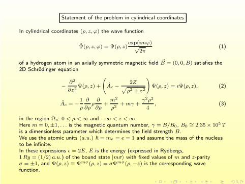
Statement of the problem in cylindrical coordinates

In cylindrical coordinates (ρ, z, ϕ) the wave function

Ψ(ρ, z, ϕ) = Ψ(ρ, z)exp(ımϕ)√

2π(1)

of a hydrogen atom in an axially symmetric magnetic field B = (0, 0, B) satisfies the2D Schrodinger equation

− ∂2

∂z2Ψ(ρ, z) +

(Ac − 2Z√

ρ2 + z2

)Ψ(ρ, z) = εΨ(ρ, z), (2)

Ac = −1

ρ

∂

∂ρρ

∂

∂ρ+

m2

ρ2+ mγ +

γ2ρ2

4, (3)

in the region Ωc: 0 < ρ < ∞ and −∞ < z < ∞.Here m = 0,±1, . . . is the magnetic quantum number, γ = B/B0, B0

∼= 2.35 × 105 Tis a dimensionless parameter which determines the field strength B.We use the atomic units (a.u.) = me = e = 1 and assume the mass of the nucleusto be infinite.In these expressions ε = 2E, E is the energy (expressed in Rydbergs,1 Ry = (1/2) a.u.) of the bound state |mσ〉 with fixed values of m and z-parityσ = ±1, and Ψ(ρ, z) ≡ Ψmσ(ρ, z) = σΨmσ(ρ,−z) is the corresponding wavefunction.

The boundary conditions in each mσ subspace of the full Hilbert space have the form

limρ→0

ρ∂Ψ(ρ, z)

∂ρ= 0, for m = 0, (4)

Ψ(0, z) = 0, for m = 0, (5)

limρ→∞ Ψ(ρ, z) = 0. (6)

The wave function of the discrete spectrum obeys the asymptotic boundary condition.Approximately this condition is replaced by the boundary condition of the first type atlarge, but finite |z| = zmax 1, namely,

limz→±∞ Ψ(ρ, z) = 0 → Ψ(ρ,±zmax) = 0. (7)

These functions satisfy the additional normalization condition

zmax∫−zmax

∞∫0

|Ψ(ρ, z)|2ρdρdz = 1. (8)

The asymptotic boundary condition for the continuum wave function will beconsidered below.

Kantorovich expansion

Consider a formal expansion of the partial solution ΨEmσi (ρ, z) of Eqs. (2)–(6),

corresponding to the eigenstate |mσi〉, expanded in the finite set of one-dimensionalbasis functions Φm

j (ρ; z)jmaxj=1

ΨEmσi (ρ, z) =

jmax∑j=1

Φmj (ρ; z)χ

(mσi)j (E, z). (9)

In Eq. (9) the functions χ(i)(z)≡ χ(mσi)(E, z), (χ(i)(z))T =(χ(i)1 (z),. . . ,χ

(i)jmax

(z))

are unknown, and the surface functions Φ(ρ; z) ≡ Φm

(ρ; z) = Φm

(ρ;−z),(Φ(ρ; z))T = (Φ1(ρ; z), . . . , Φjmax (ρ; z)) form an orthonormal basis for each value ofthe variable z which is treated as a parameter.

In the KM the wave functions Φj(ρ; z) and the potential curves Ej(z) (in Ry) aredetermined as the solutions of the following eigenvalue problem

AcΦj(ρ; z) = Ej(z)Φj(ρ; z), (10)

with the boundary conditions

limρ→0

ρ∂Φj(ρ; z)

∂ρ= 0, for m = 0, and Φj(0; z) = 0, for m = 0,(11)

limρ→∞ Φj(ρ; z) = 0. (12)

Since the operator in the left-hand side of Eq. (10) is self-adjoint, its eigenfunctionsare orthonormal⟨

Φi(ρ; z)

∣∣∣∣Φj(ρ; z)

⟩ρ

=

∫ ∞

0Φi(ρ; z)Φj(ρ; z)ρdρ = δij , (13)

where δij is the Kronecker symbol.

Therefore we transform the solution of the above problem into the solution of aneigenvalue problem for a set of jmax ordinary second-order differential equations thatdetermines the energy ε and the coefficients χ(i)(z) of the expansion (9)(

−Id2

dz2+ U(z) + Q(z)

d

dz+

dQ(z)

dz

)χ(i)(z) = εi Iχ

(i)(z). (14)

Here I, U(z) = U(−z) and Q(z) = −Q(−z) are the jmax × jmax matrices whoseelements are expressed as

Uij(z) =

(Ei(z) + Ej(z)

2

)δij + Hij(z), Iij = δij ,

Hij(z) = Hji(z) =

∫ ∞

0

∂Φi(ρ; z)

∂z

∂Φj(ρ; z)

∂zρdρ, (15)

Qij(z) = −Qji(z) = −∫ ∞

0Φi(ρ; z)

∂Φj(ρ; z)

∂zρdρ.

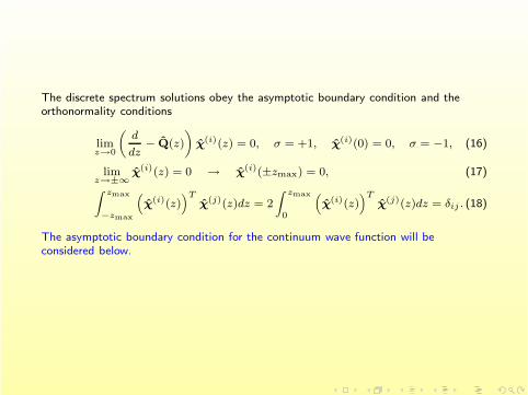
The discrete spectrum solutions obey the asymptotic boundary condition and theorthonormality conditions

limz→0

(d

dz− Q(z)

)χ(i)(z) = 0, σ = +1, χ(i)(0) = 0, σ = −1, (16)

limz→±∞ χ(i)(z) = 0 → χ(i)(±zmax) = 0, (17)∫ zmax

−zmax

(χ(i)(z)

)Tχ(j)(z)dz = 2

∫ zmax

0

(χ(i)(z)

)Tχ(j)(z)dz = δij . (18)

The asymptotic boundary condition for the continuum wave function will beconsidered below.

Algorithm 1 of generation of parametric algebraic problems by theFinite Element Method

To solve eigenvalue problem for equation (10) the boundary conditions (11), (12) andthe normalization condition (13) with respect to the space variable ρ on an infiniteinterval are replaced with appropriate conditions (11), (13) and Φ(ρmax; z) = 0 on afinite interval ρ ∈ [ρmin ≡ 0, ρmax].We consider a discrete representation of solutions Φ(ρ; z) of the problem (10) bymeans of the FEM on the grid, Ωp

h(ρ)= (ρ0 =ρmin, ρj = ρj−1 + hj , ρn =ρmax), in a

finite sum in each z = zk of the grid Ωph(z)

[zmin, zmax]:

Φ(ρ; z) =

np∑µ=0

Φhµ(z)Np

µ(ρ) =n∑

r=0

p∑j=1

Φhr+p(j−1)(z)Np

r+p(j−1)(ρ), (19)

where Npµ(ρ) are local functions and Φh

µ(z) are node values of Φ(ρµ; z). The localfunctions Np

µ(ρ) are piece-wise polynomial of the given order p equals one only in thenode ρµ and equals zero in all other nodes ρν = ρµ of the grid Ωp

h(ρ), i.e.,

Npν (ρµ) = δνµ, µ, ν = 0, 1, . . . , np. The coefficients Φν(z) are formally connected

with solution Φ(ρpj,r ; z) in a node ρν = ρp

j,r , r = 1, . . . , p, j = 0, . . . , n:

Φhν (z) = Φh

r+p(j−1)(z) ≈ Φ(ρpj,r ; z), ρp

j,r = ρj−1 +hj

pr.

The theoretical estimate for the H0 norm between the exact and numerical solutionhas the order of

|Ehm(z) − Em(z)| ≤ c1|Em(z)| h2p,

∥∥∥Φhm(z) − Φm(z)

∥∥∥0≤ c2|Em(z)|hp+1,

where h = max1<j<n hj is maximum step of grid. It has been shown that we have apossibility to construct schemes with high order of accuracy comparable with thecomputer one. Let us consider the reduction of differential equations (10) on theinterval ∆ : ρmin < ρ < ρmax with boundary conditions in points ρmin and ρmax

rewriting in the form

A(z)Φ(ρ; z) = E(z)B(z)Φ(ρ; z), (20)

where A and B are differential operators. Substituting expansion (19) to (20) andintegration with respect to ρ by parts in the interval ∆ = ∪n

j=1∆j , we arrive to asystem of the linear algebraic equations

apµνΦh

µ(z) = E(z)bpµνΦh

µ(z), (21)

in framework of the briefly described FEM. Using p-order Lagrange elements, wepresent below an algorithm 1 for construction of algebraic problem (21) by the FEM inthe form of conventional pseudocode. It MAPLE realization allow us show explicitlyrecalculation of indices µ, ν and test of correspondent modules in FORTRAN code.

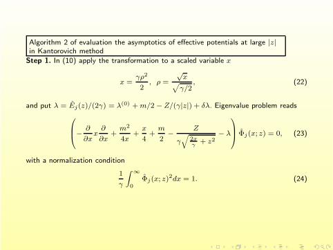
Algorithm 2 of evaluation the asymptotics of effective potentials at large |z|in Kantorovich method

Step 1. In (10) apply the transformation to a scaled variable x

x =γρ2

2, ρ =

√x√

γ/2, (22)

and put λ = Ej(z)/(2γ) = λ(0) + m/2 − Z/(γ|z|) + δλ. Eigenvalue problem reads− ∂

∂xx

∂

∂x+

m2

4x+

x

4+

m

2− Z

γ√

2xγ

+ z2− λ

Φj(x; z) = 0, (23)

with a normalization condition

1

γ

∫ ∞

0Φj(x; z)2dx = 1. (24)

At Z = 0 Eq. (23) takes the form

L(n)Φ(0)nm(x) = 0, L(n) = − ∂

∂xx

∂

∂x+

m2

4x+

x

4− λ(0), (25)

and has the regular and bounded solutions at

λ(0) = n + (|m| + 1)/2, (26)

where transverse quantum number n ≡ Nρ = j − 1 = 0, 1, . . . determines the numberof nodes of the solution Φ

(0)nm(x) with respect to the variable x. Normalized solutions

of Eq. (25), take the form

Φ(0)nm(x) = Cn|m|e−

x2 x

|m|2 L

|m|n (x), Cn|m| =

[γ

n!

(n + |m|)!] 1

2, (27)

1

γ

∫ ∞

0Φ

(0)nm(x)Φ

(0)n′m(x)dx = δnn′ , (28)

where L|m|n (x) are Laguerre polynomials.

Step 2.

Substituting notationδλ = λ − λ(0) − m/2 + Z/(γ|z|) ≡ Ej(z)/(2γ) − (n + (m + |m| + 1)/2) + Z/(γ|z|),and decomposition

Z

γ|z| −Z

γ√

2xγ

+ z2=

jmax∑k=1

V (k)

|z|k ,

V (k) =

−(−1)k′ (2k′−1)!!

k′!Zxk′

γk′+1 , k = 2k′ + 1, k′ = 1, 2, . . . ,

0, otherwise,

to Eq. (23) at Z = 0, transform it in the following form

L(n)Φj(x; z) +

jmax∑

k=1

V (k)

|z|k − δλ

Φj(x; z) = 0. (29)

Step 3.

Solution of equation (29) is found in the form of the perturbation series by inversepowers of |z|

δλ =

kmax∑k=0

|z|−kλ(k), Φj(x; z) =

kmax∑k=0

|z|−kΦ(k)n (x). (30)

Equating coefficients at the same powers of |z|, we arrive to the system ofinhomogeneous differential equations with respect to corrections λ(k) and Φ(k)

L(n)Φ(0)(x) = 0 ≡ f(0),

L(n)Φ(k)(x) =

k−1∑p=0

(λ(k−p) − V (k−p))Φ(p)(x) ≡ f(k), k ≥ 1. (31)

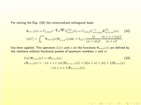
For solving the Eqs. (29) the unnormalized orthogonal basis

Φn+s(x) = Cn|m|e−x2 x

|m|2 L

|m|n+s(x) = Cn|m|C

−1n+s|m|Φ

(0)n+s,m(x), (32)

〈s|s′〉 =

∫ ∞

0Φn+s(x)Φn+s′ (x)dx = δss′γ

n!

(n + |m|)!(n + s + |m|)!

(n + s)!,

has been applied. The operators L(n) and x on the functions Φn+s(x) are defined bythe relations without fractional powers of quantum numbers n and m

L(n)Φn+s(x) = sΦn+s(x), (33)

xΦn+s(x) = −(n + s + |m|)Φn+s−1(x) + (2(n + s) + |m| + 1)Φn+s(x)

−(n + s + 1)Φn+s+1(x).

Step 4.

Applying relations (33), the right-hand side f(k) and solutions Φ(k)(x) of the system(31) are expanded over basis states Φn+s(x)

Φ(k)n (x) =

k∑s=−k

b(k)s Φn+s(x), f(k) =

k∑s=−k

f(k)s Φn+s(x). (34)

Then a recurrent set of linear algebraic equations for unknown coefficients b(k)s and

corrections λ(k) is obtained

sb(k)s − f

(k)s = 0, s = −k, . . . , k.

that is solved sequentially for k = 1, 2, . . . , kmax:

f(k)0 = 0 → λ(k); b

(k)s = f

(k)s /s, s = −k, . . . , k, s = 0.

The initial conditions (26) and b(0)s = δs0 are followed from (25) and (28).

Step 5.

To obtain the normalized wave function Φj(x; z) up to the k-th order, the coefficientb(k)0 are defined by the following relation:

b(k)0 = − 1

2γ

k−1∑p=1

k−p∑s′=p−k

p∑s=−p

b(k−p)s 〈s|s′〉b(p)

s′ , b(k=1,...,5)0 = 0.

As an example of output file at steps 1–5, we display nonzero coefficients λ(k), b(k)s of

the inverse power series (30), (34) up to O(|z|−5):

λ(0) = n + (|m| + 1)/2, λ(3) = Z(2n + |m| + 1)/γ2,

b(0)0 = 1, b

(3)−1 = −Z(n + |m|)/γ2, b

(3)1 = Z(n + 1)/γ2. (35)

Step 6.

In scaled variable x the relations of effective potentials Hij(z) = Hji(z) andQij(z) = −Qji(z) takes form

Hij(z)=1

γ

∞∫0

dx∂Φi(x; z)

∂z

∂Φj(x; z)

∂z, Qij(z)=− 1

γ

∞∫0

dxΦi(x; z)∂Φj(x; z)

∂z. (36)

For their evaluation the decomposition of solution Eqs. (25) over the normalizedorthogonal basis Φ

(0)n+s with the normalized coefficients b

(k)n;n+s,

Φ(k)n (x) =

k∑s=−k

b(k)n;n+sΦ

(0)n+s, (37)

has been applied. The normalized coefficients b(k)n;n+s are calculated via b

(k)s ,

b(k)n;n+s = b

(k)s

√n!

(n + |m|)!(n + s + |m|)!

(n + s)!(38)

as follows from (34), (37) and (32).

Step 7.

In a result of substitution (30), (37) in (36), matrix elements takes form

Qjj+t(z) = −kmax−1∑

k=0

|z|−k−1k∑

k′=0

min(k,k−k′−t)∑s=max(−k,k′−k−t)

(k − k′)b(k′)

n;n+sb(k−k′)n+t;n+s,

Hjj+t(z) =

kmax−2∑k=0

|z|−k−2k∑

k′=0

min(k,k−k′−t)∑s=max(−k,k′−k−t)

k′(k − k′)b(k′)

n;n+sb(k−k′)n+t;n+s. (39)

Collecting of coefficients of (39) at equal powers of |z|, algorithm leads to finalexpansions of eigenvalues and effective potentials of output file

Ej(z) =

kmax∑k=0

|z|−kE(k)j , Hij(z) =

kmax∑k=8

|z|−kH(k)ij , Qij(z) =

kmax∑k=4

|z|−kQ(k)ij . (40)

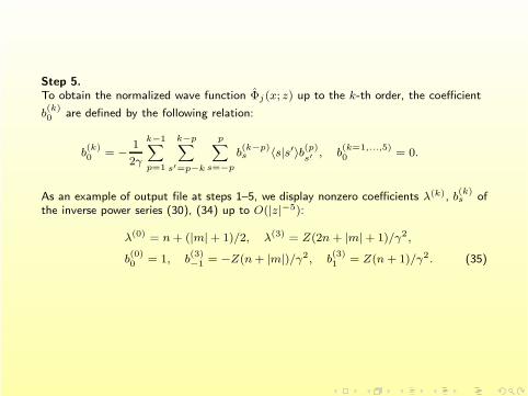
The successful run of the above algorithm was occurs up to kmax = 16 (Run time is95s on Intel Pentuim IV, 2.40 GHz, 512 MB). The some first nonzero coefficientstakes form (j = n + 1)

E(0)j = 2γ(n + (m + |m| + 1)/2),

E(1)j = −2Z,

E(3)j = 2Z(2n + |m| + 1)/γ,

E(5)j = −3Z(2 + 3|m| + 6n2 + |m|2 + 6n|m| + 6n)/γ2,

E(6)j = −2Z2(2n + |m| + 1)/γ3,

Q(4)jj+1 = 3Z

√n+1

√n+|m|+1/γ2,

Q(6)jj+1 = −15Z

√n+1

√n+|m|+1(2n + |m| + 2)/γ3,

Q(6)jj+2 = 15Z

√n+1

√n+2

√n+|m|+1

√n+|m|+2/(4γ3),

H(8)jj = 9Z2(2n2 + 2n|m| + 2n + |m| + 1)/γ4,

H(10)jj = −90Z2(2n + |m| + 1)(2n2 + 2n|m| + 2n + |m| + 2)/γ5,

H(10)jj+1 = 45Z2

√n+1

√n+|m|+1(n2 + n|m| + 2n + |m| + 2)/(2γ5),

H(8)jj+2 = −9Z2

√n+1

√n+2

√n+|m|+1

√n+|m|+2/γ4,

H(10)jj+2 = 90Z2

√n+1

√n+2

√n+|m|+1

√n+|m|+2(2n + |m| + 3)/γ5,

H(10)jj+3 = −45Z2

√n+1

√n+2

√n+3

√n+|m|+1

√n+|m|+2

√n+|m|+3/(2γ5).

0,0 0,5 1,0 1,5 2,00

20

40

60

80

100

120E6

E5

E4

E3

E2

E

z

E1

0,0 0,2 0,4 0,6 0,8 1,00,00

0,01

0,02

0,03

0,04

0,05

0,06

0,07

H

z

H66H55H44H33H22H11

0,0 0,5 1,0 1,5 2,00,00

0,04

0,08

0,12

0,16

Q

z

Q34

Q23

Q12

Q24

Q13

Q14

0,0 0,2 0,4 0,6 0,8 1,0-0,02

-0,01

0,00

0,01

0,02

0,03

H24H14H13

H

z

H34H23H12

The behaviour of potential curves Ej(z), effective potentials Qij(z) and Hij(z) forγ = 10, m = −1.

Values of the partial sums (40) depending on kmax for m = −1,Z = 1, z = 10, γ = 10. The last row contains the corresponding numerical values (n.v.).

i, j Q12, 10−6 Q23, 10−6 Q34, 10−5 Q13, 10−8 Q24, 10−8

z −4Q( 4)ij 4.24264069 7.34846923 1.03923048 0 0

+z −6Q( 6)ij 4.17900108 7.16475750 1.00285742 1.29903811 3.18198052

+z −7Q( 7)ij 4.17883137 7.16446356 1.00281585 1.29903811 3.18198052

+z −8Q( 8)ij 4.17972233 7.16857870 1.00394341 1.26266504 3.04833733

+z −9Q( 9)ij 4.17972824 7.16859579 1.00394680 1.26260268 3.04818460

+z−10Q(10)ij 4.17971489 7.16850321 1.00391243 1.26342108 3.05252800

+z−11Q(11)ij 4.17971474 7.16850253 1.00391224 1.26342451 3.05254060

+z−12Q(12)ij 4.17971496 7.16850469 1.00391330 1.26340651 3.05240830

+z−13Q(13)ij 4.17971496 7.16850471 1.00391331 1.26340638 3.05240762

+z−14Q(14)ij 4.17971496 7.16850466 1.00391328 1.26340679 3.05241163

+z−15Q(15)ij 4.17971496 7.16850466 1.00391327 1.26340679 3.05241166

+z−16Q(16)ij 4.17971496 7.16850466 1.00391328 1.26340678 3.05241154

(n.v.) 4.17971496 7.16850466 1.00391328 1.26340678 3.05241154

Algorithm 3 of evaluation the asymptotics of solutions at large |z| in Kantorovich method

Step 1. We write the set of differential equations (14) at fixed values m, and ε in theexplicit form for χjio (z) ≡ χ

(io)j (z) and j = 1, 2, . . . , jmax, io = 1, 2, . . . , No

−d2χjio (z)

dz2− 2Z

|z| χjio (z) −(

ε − Ej(z) − 2Z

|z|)

χjio(z) + Hjj(z)χjio (z)

=

jmax∑j′=1,j′ =j

(−Qjj′ (z)

d

dz− Hjj′ (z) − dQjj′ (z)

dz

)χj′io

(z), (41)

where matrix elements Qjj′ (z) and Hjj′ (z) have of the form (40).

Note, that at large z, E(2)i =H

(2)ii =0, i.e., the centrifugal terms are eliminated and

the longitudinal solution has the asymptotic form corresponding to zero angularmomentum solutions, or to the one-dimensional problem on a semi-axis:

χjio (z) =exp(w(z))√

pio

φjio (z), φjio (z) =

kmax∑k=0

φ(k)jio

|z|−k, (42)

where w(z) = ıpio |z|+ ıζ ln(2pio |z|) + ıδio , pio is the momentum in the channel, ζ isthe characteristic parameter, and δio is the phase shift.

The components φ(k)jio

satisfy the system of ordinary differential equations

(p2io

− 2E + E(0)j )φ

(k)jio

= f(k)jio

(φ(k′=0,...,k−1)j′io

, pio)

≡ −2(ζpio + ı(k − 1)pio − Z)φ(k−1)jio

− (ζ + ı(k − 2))(ζ + ı(k − 1))φ(k−2)jio

−k∑

k′=3

(E(k′)j + H

(k′)jj )φ

(k−k′)jio

+

jmax∑j′=1

k∑k′=4

(−2ıQ(k′)jj′ pio − H

(k′)jj′ )φ

(k−k′)j′io

+

jmax∑j′=1

k∑k′=5

(2k − 1 − k′ − 2ıζ)Q(k′−1)jj′ φ

(k−k′)j′io

,

k = 0, 1, . . . , kmax, φ(−1)jio

≡ 0, φ(−2)jio

≡ 0, kmax ≤ jmax − io. (43)

Here index of summation, j′, takes integer values, except io and j, (j′ = 1, . . . ,jmax, j′ = io, j′ = j).

Step 2.

From first two equations (k = 0, 1) of set (43) we have the leading terms ofeigenfunction φ

(0)jio

, eigenvalue p2io

and characteristic parameter ζ, i.e initial data forsolving recurrence sequence,

φ(0)jio

= δjio , p2io

= 2E − E(0)io

→ pio =

√2E − E

(0)io

, ζ = Z/pio . (44)

Open channels have p2io

≥ 0, and close channels have p2io

< 0. Lets there areNo ≤ jmax open channels, i.e., p2

io≥ 0 for io = 1, . . . No and p2

io< 0 for

io = No + 1, . . . jmax.

Step 3.

Substituting (44) in (43), we obtain the following recurrent set of algebraic equationsfor the unknown coefficients φjio (z) for k = 1, 2, . . . , kmax:

(E(0)io

− E(0)j )φ

(k)jio

= f(k)jio

(φ(k′=0,...,k−1)j′io

, pio ) (45)

that is solved sequentially for k = 1, 2, . . . , kmax:

φ(k)jio

= f(k)jio

(φ(k′=0,...,k−1)j′io

, pio)/(E(0)io

−E(0)j ), j = io,

f(k+1)ioio

(φ(k′=0,...,k)j′io

, pio) = 0 → φ(k)ioio

. (46)

The successful run of the above algorithm was occurs up to kmax = 16 (Run time is167s on Intel Pentuim IV, 2.40 GHz, 512 MB). The some first nonzero coefficientstakes form (j = n + 1)

φ(0)jio

= δjio ,

φ(1)jio

= δjio ıZ(Z+ıpio)/(2p3io

),

φ(2)jio

= δjio [ıE(3)j /(4pio )−Z(Z+ıpio)2(Z+2ıpio )/(8p6

io)],

φ(3)jio

= δjio [−E(3)j (3Z2+7ıpioZ−6p2

io)/(24p4

io)

−ıZ(Z+ıpio)2(Z+2ıpio)2(Z+3ıpio)/(48p9io

)],

φ(4)jio

= δjio [ıE(5)j /(8pio )−(E

(3)j )2/(32p2

io)

−ıE(3)j (3Z4+20ıpioZ3−53p2

ioZ2−66ıp3

ioZ+36p4

io))/(96p7

io)

+Z(Z+ıpio)2(Z+2ıpio )2(Z+3ıpio)2(Z+4ıpio )/(384p12io

)]

+2ıpioQ(4)jio

/(E(0)io

−E(0)j ).

Remarks:

1. Expansion (42) holds true for |zm| max(Z2/(2p3io

), 2Z(2io + |m| − 1)/(8γp2io

)).The choice of a new value of zmax for the constructed expansions of the linearlyindependent solutions for pio > 0 is controlled by the fulfillment of the Wronskiancondition with a long derivative Dz ≡ Id/dz − Q(z)

Wr(Q(z); χ∗(z), χ(z)) = (χ∗(z))T Dzχ(z) − (Dzχ∗(z))T χ(z) = 2ıIoo

up to the prescribed accuracy. Here Ioo is the No-by-No identity matrix.2. This algorithm can be applied also for evaluation asymptotics of solutions in closedchannels pio = ıκio , κio > 0.

Applications algorithms for solving the eigenvalue problem

The symbolic-numerical algorithms are used to generate an input file of effectivepotentials in the Gaussian points z = zk of the FEM grid Ωp

h(z)[zmin = 0, zmax] and

asymptotic of solutions of a set of longitudinal equations (14)–(18) for the KANTBPcode (Chuluunbaatar, O., et al: KANTBP: A program for computing energy levels,reaction matrix and radial wave functions in the coupled-channel hypersphericaladiabatic approach. accepted in Comput. Phys. Commun. (2007)). The calculationswas performed on a grid Ωp

h(z)= 0(200)2(600)150 (the number in parentheses

denotes the number of finite elements of order p = 4 in each interval). Comparisonwith corresponding calculations given in spherical coordinates from (Dimova, M.G.,Kaschiev, M.S., Vinitsky, S.I.: The Kantorovich method for high-accuracy calculationsof a hydrogen atom in a strong magnetic field: low-lying excited states. Journal ofPhysics B: At. Mol. Phys. 38 (2005) 2337–2352) given in the last line of the Table isshown that elaborated method in cylindrical coordinates is applicable for strengthmagnetic field γ > 5 and magnetic number m of order of ∼ 10.Convergence of the method for the binding energy E = γ/2 − E (in a.u.) of even wavefunctions m = −1, γ = 10 and γ = 5 versus the number jmax of coupled equations.

jmax 2p−1 (γ = 10) 3p−1 (γ = 10) 2p−1 (γ = 5) 3p−1 (γ = 5)1 1.123 532 554 (3) 0.182 190 992 (2) 0.857 495 336 (9) 0.165 082 403 (4)2 1.125 069 513 (1) 0.182 282 868 (7) 0.859 374 058 (2) 0.165 234 428 (1)3 1.125 280 781 (8) 0.182 294 472 (5) 0.859 641 357 (6) 0.165 253 152 (9)4 1.125 343 075 (2) 0.182 297 825 (6) 0.859 721 942 (4) 0.165 258 606 (4)6 1.125 381 347 (9) 0.182 299 867 (7) 0.859 772 441 (3) 0.165 261 973 (6)8 1.125 392 776 (1) 0.182 300 474 (6) 0.859 787 833 (7) 0.165 262 991 (9)10 1.125 397 502 (9) 0.182 300 725 (2) 0.859 794 289 (0) 0.165 263 418 (0)12 1.125 399 854 (7) 0.182 300 849 (8) 0.859 797 533 (8) 0.165 263 631 (9)

1.125 422 341 (8) 0.182 301 494 (7) 0.859 832 622 (6) 0.165 264 273 (1)

Conclusion

• A set of symbolic-numerical algorithms for calculating wave functions of a hydrogenatom in a strong magnetic field is developed. The method is based on the Kantorovichapproach to parametric eigenvalue problems in cylindrical coordinates.•The rate of convergence of the Kantorovich expansion is examined numerically andillustrated by a set of typical examples. The results are in a good agreement withcalculations executed in spherical coordinates at fixed m for γ > 5.•The elaborated symbolic-numerical algorithms for calculating effective potentials andasymptotic solutions allows us to generate effective approximations for a finite set oflongitudinal equations describing an open channel to have the low upper estimations.

• The main goal of the method consists in the fact that for states having preferably acylindrical symmetry a convergence rate is increased at fixed m with growing values ofγ 1 or the high-|m| Rydberg states at |m| > 150 in laboratory magnetic fieldsB = 6.10T (γ = 2.595 · 10−5 a.u.), such that several equations are provide a givenaccuracy.•The developed approach yields a useful tool for calculation of threshold phenomenain formation and ionization of (anti)hydrogen like atoms and ions in magnetic trapsand channeling of ions in thin films .This work was partly supported by the Russian Foundation for Basic Research (grantNo. 07-01-00660) and by Grant I-1402/2004-2007 of the Bulgarian Foundation forScientific Investigations.