A th I t t ti f B tht b CAnother Interpretation of Bathtub Curve

Hi T b ki (t b ki@i j )Hiroe Tsubaki (tsubaki@ism.ac.jp)Director, Risk Analysis Research Centre,The Institute of Statistical Mathematics

The Erl King" by Albert Sterner ca 1910 The Oldest Twins; Kin san Gin sanThe Erl King , by Albert Sterner, ca. 1910http://www.answers.com/topic/der-erlk-nig

The Oldest Twins; Kin-san Gin-san

http://www.geocities.co.jp/SilkRoad-Ocean/2002/nati0000.htm

2012/07 1

ContentsContents

• The Grammar of Science– Classification before modelingg

• Three Case StudiesR id l A l i f R i f– Residual Analysis of Regression of non-anonymized data

– Analysis of Outliers – Another Interpretation of Bathtub Curvep

• Mixture of Normal, Weak and Strong Populations

• Concluding Remarks• Concluding Remarks2012/07 2

Two Typical Misinterpretations to Science & StatisticsTwo Typical Misinterpretations to Science & Statistics

• Business is beyond the scope of Science• Why Business Sciences?

B i i t i l f i !– Business is material for science!

– Statistics is a kind of applied mathematics • Why Statistical Methodology?• Why Statistical Methodology?

– Statistics is the grammar of science

2012/07 3

Definition of ScienceDefinition of ScienceTh k h• The attempt to make the chaotic diversity of our our sense experiencesense experiencecorrespond to a logically uniform system of thought

A Einstein 1940– A. Einstein, 1940

Akademie Olympia

2012/07 4

Statistical ScienceStatistical Science

T di th d f• To discover methods of condensing information concerning large groups g g g pof allied facts into brief and compendious expressionsexpressions suitable for discussion– Francis Galton (1883)

• Inquiries into Human Faculty and its Developmentp

http://www mugu com/galton/2012/07 5

http://www.mugu.com/galton/

Business is also material for scienceBusiness is also material for science• Karl Pearson, 1892

• The unity of all scienceThe unity of all science consists in its method, not in its material.

• The field of science is unlimited; its material is endless, every group of natural phenomena, every phase of social life everyphase of social life, every stage of past or present development is material for science.

• The man who classifies fact of any kind whatever, who sees their mutual relations and d ib th i idescribes their consequences, is applying the scientific method and is a man of science

d t d k/ hi t /M th ti i /P ht l

2012/07 6

www-groups.dcs.st-and.ac.uk/ ~history/Mathematicians/Pearson.html

Karl Pearson (1892) The Grammar of Science• A man gives a law to Nature

– Statistical Science as “a new way” to Scientific thinkingy• Systematic ways to derive a scientific law ( = model)• Not Scientific Objects but Scientific Process

– Model Planning: Statistical Methods for PlanningModel Planning: Statistical Methods for Planning» Careful and accurate classification of facts» Observation of their correlation and sequence

– Do (Fitting Model) : Constructing Scientific Laws– Do (Fitting Model) : Constructing Scientific Laws » Discovery of scientific laws by aid of creative imagination

– C: Checking the Laws» Self criticism and the final touchstone of equal validity for all» Self-criticism and the final touchstone of equal validity for all

normally constituted minds• Development of Statistical Methodology as the Supporting tools

for the Grammarfor the Grammar– Statistical and Probabilistic interpretation of causes and effects– Statistical description of a scientific law

2012/07 7

1.0

Case Studies

60.

80.

40.

60.

00.

2

Cob-Douglas Production Function and Prediction of P fit bilit f J Li t d E t i

0.0e+00 5.0e+06 1.0e+07 1.5e+07

Profitability for Japanese Listed Enterprises

Sales Incomes and Profitability are hypotheticallySales Incomes and Profitability are hypothetically regarded as Survival Time

2012/07 8

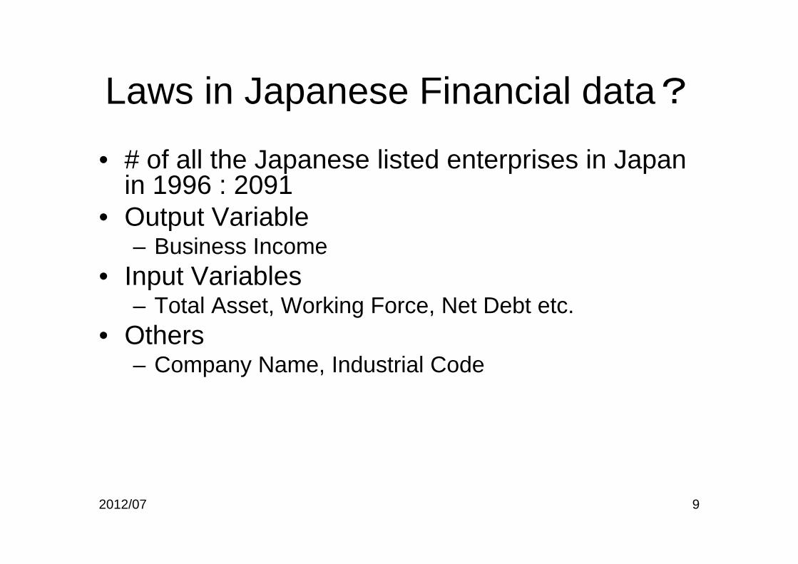
Laws in Japanese Financial data？Laws in Japanese Financial data？

# f ll th J li t d t i i J• # of all the Japanese listed enterprises in Japan in 1996 : 2091

• Output Variable• Output Variable– Business Income

• Input VariablesInput Variables– Total Asset, Working Force, Net Debt etc.

• Others– Company Name, Industrial Code

2012/07 9

Description of DispersionSales Income

Histogram of log(BusinessIncome)

Histogram of BusinessIncome

2000

Histogram of log(BusinessIncome)

500

600

ncy

1500 Mean：¥195400million

sd：¥857400million Freq

uenc

y

200

300

400

Mean:10.9 sd:1.40

Geometric Mean:

Freq

uen

500

1000

8 10 12 14 16

010

0 ¥52560million

BusinessIncome

0.0 e+00 5.0 e+06 1.0 e+07 1.5 e+07

0

log(BusinessIncome)

67

Normal Q-Q Plot

45

6

Sam

ple

Qua

ntile

s

2012/07 10-3 -2 -1 0 1 2 3

3

Theoretical Quantiles

STEP 1 PlanningDescription of Association

e+07

e+07

Linear relationship?Log Linear relationship!

e+0

71.5

1 e

+06

1 e

Ｒ２＝０．１８ Ｒ２＝０．７２

e+06

1.0

Bus

iness

Incom

e

1

e+05

1

Bus

iness

Incom

e

e+00

5.0

e+0

31 e+04

0 50000 100000 150000

0.0 e

WorkingForce

5 e+01 5 e+02 5 e+03 5 e+041

e

WorkingForce

2012/07 11

Step 2: Model FittingStep 2: Model Fitting

Fitti th d l th h th ti l l t• Fitting the model or the hypothetical law to the related facts (data) to get the empirical law– Regression Analysis

• Log (Sales Income)=4.24+0.97 log (Working Force)+residualsstandard deviation of residual=0 74standard deviation of residual=0.74

– sd of log Business Income = 1.40

2012/07 12

Fitting ModelFitting Model

Original Variation

1416

)1015

Variation of R id l

012

log(

Bus

ines

sInc

ome

5

Residuals

810

0

4 6 8 10 12

log(WorkingForce)

1 2

2012/07 13

Step 3: Checking the Fitted ModelStep 3: Checking the Fitted Model

Ch ki f f th bt i d l t• Checking performance of the obtained law to clarify the needs of classification of the facts– DiagnosticsDiagnostics

• Total Performance Measures of the model– R2, Residual SD

• Exploring Needs for Further Classification• Exploring Needs for Further Classification– Residual Analysis

2012/07 14

Evolution of ModelEvolution of Model

L (SI) 1 15 R id l f• Log(SI)=1.15+0.28 log(WF)+0.46log(Total Assets)

Residuals of the simple model

Residuals of the new modelg( )

+0.27log(Net Debt)+residuals

R2 0 89

34

– R2=0.89residual SD=0.47

• Residuals SD of the simple model =0 74 0

12

simple model =0.74• Total performance of the

prediction model is significantly improved -2-1

0

significantly improved.

1 2

2012/07 15

Residual Analysis Clarifies Needs of Classification:Companies such that the residuals>1.5

1500 ITOCHU 1 854051• 1500 ITOCHU 1.854051• 1501 Marubeni 1.853562• 1502 TOMEN 1.835570• 1503 Nichimen 1.670540• 1518 KANEMATSU 1.761537• 1528 CHUO GYORUI 2.258017• 1529 MITSUI & CO. 1.660330• 1536 TOHTO SUISAN 2 064938• 1536 TOHTO SUISAN 2.064938• 1537 TSUKIJI UOICHIBA 1.967221• 1539 OSAKA UOICHIBA 1.878274• 1542 DAITO GYORUI 2.032328• 1548 SUMITOMO 1.960161• 1557 Nissho Iwai 1.662237• 1564 TOKYO SANGYO 2.552716• 1625 CHUBU SUISAN 1 769532• 1625 CHUBU SUISAN 1.769532• 2090 SHINKO GYORUI 2.031702

2012/07 16

Companies such that the residuals< 1 3Companies such that the residuals< -1.3

• 9 Chugai Mining 1 521919• 9 Chugai Mining -1.521919• 480 KYOWA HAKKO KOGYO -1.392347• 548 Green Cross -1.819432• 568 INTERNATIONAL REAGENTS -1.557378• 955 ISEKI & CO -1 372723• 955 ISEKI & CO. -1.372723• 1142 SANYO ELECTRIC -1.338558• 1762 HOKKAIDO SHINKO -1.536938• 1781 TOBU RAILWAY -1.322300• 1786 Keihin Electric Express Railway -1 354466• 1786 Keihin Electric Express Railway -1.354466• 1787 Odakyu Electric Railway -1.333317• 1789 Keisei Electric Railway -1.389206• 1798 Kinki Nippon Railway -1.387198• 1800 HANSHIN ELECTRIC RAILWAY -1 381091• 1800 HANSHIN ELECTRIC RAILWAY -1.381091• 1801 Nankai Electric Railway -1.490005• 1803 Kobe Electric Railway -1.667814• 1804 Nagoya Railroad -1.348491• 1807 Sanyo Electric Railway -1 558611• 1807 Sanyo Electric Railway 1.558611• 1876 Nihonbashi Warehouse -1.327809• 1945 WESCO -1.861918• 1954 Koshien Tochi Kigyo -1.340120• 1980 KYOTO HOTEL -1 328580

2012/07 17

1980 KYOTO HOTEL 1.328580

Needs for ClassificationNeeds for Classification

Aft Cl ifi ti• After Classification– Commerce (#181):

• ~0.27+0.08logWF+0.77logTA+0.21logND– Residual SD: 0.51 R2:0.89

(# 1)– Transportation(#51)：• ~1.86+0.64logWF+0.59logTA-0.24logND

R id l SD 0 35 R2 0 93– Residual SD: 0.35 R2:0.93

– Others：1 26+0 38logWF+0 40logTA+0 24logND• ~1.26+0.38logWF+0.40logTA+0.24logND– Residual SD: 0.38 R2:0.92

• But if Data were anonymized?2012/07 18

• But if Data were anonymized?.

Analysis of Residuals by Rank Logit ModelingAnalysis of Residuals by Rank Logit Modeling

• Qualitative Choice by Ascending Order– Proportional Hazard Model: Weak population

• Log(f/(1-F))=log λ(t) + βTX– Erl-king Selects Children.

Q li i Ch i b D di O d• Qualitative Choice by Descending Order– Proportional Reverse Hazard Model: Strong Population

T• Log(f/F)=log ρ(t) + βTX– God Celebrates Kinsan and Ginsan： Amadeus

Rank Order Logit Regression of Residuals (Ascending Order)

coef exp(coef)se(coef) z p• log(CurrentAsset) 0.048 1.05 0.048 1.006 0.310• log(LongTermAsset) -0.097 0.90 0.035 -2.765 0.005• log(LongTermDebt + 0.5) -0.000 0.99 0.006 -0.117 0.910• log(CurrentDebt) -0.096 0.90 0.049 -1.941 0.052• log(PersonnelExpense) However 0.142 1.15 0.038 3.732 0.000• log(AdvertiseExpenses+0.5) 0.004 1.00 0.006 0.666 0.510log(AdvertiseExpenses+0.5) 0.004 1.00 0.006 0.666 0.510• log(Exp&ResearchExp+0.5) 0.024 1.02 0.006 3.680 0.000• Wald test = 40.7 on 7 df, p=9.31e-07• Red: Accelerating Negative ResidualsRed: Accelerating Negative Residuals• If the residuals greater than i-th quartile could be regarded as censored data, the

Wald test statistics become– i=1 Wald Statistics = 10.5 (P Value = 0.161)( )– i=2 Wald Statistics = 10.9 (P Value = 0.143)– i=3 Wald Statistics = 28.0 (P Value = 0.0001)– i=4 Wald Statistics = 40.7 (P Value = 9.31e-07)

• Should all the data be commonly regarded as complete data? No!2012/07 20

Rank Order Logit Regression (Proportional Reverse Hazard Modeling )(Proportional Reverse Hazard Modeling )

of Residuals (Descending Order)• coef exp(coef) se(coef) z p

• log(CurrentAsset) -0.027 0.97 0.048 -0.565 5.7e-01• log(LongTermAsset) -0.030 0.97 0.032 -0.967 3.3e-01• log(LongTermDebt + 0.5) -0.001 0.99 0.006 -0.278 7.8e-01• log(CurrentDebt) -0.093 0.91 0.047 -1.948 5.1e-02• log(PersonnelExpense) 0.129 1.13 0.032 3.939 8.2e-05• log(AdvertiseExpense+0.5) 0.007 1.00 0.007 1.014 3.1e-01log(AdvertiseExpense+0.5) 0.007 1.00 0.007 1.014 3.1e 01• log(ExperimentalAndResearchExpense+0.5) 0.033 1.03 0.006 5.257 1.5e-07

• Wald test = 56.1 on 7 df, p=8.93e-10• If we regarded the residuals less than i-th quartile as censoring, the Wald test g q g,

statistics become–– i=1 Wald Statistics = 64.8 (P Value = 1.65ei=1 Wald Statistics = 64.8 (P Value = 1.65e--11)11)– i=2 Wald Statistics = 21.5 (P Value = 0.0031)i 2 Wald Statistics 21.5 (P Value 0.0031)– i=3 Wald Statistics = 18.9 (P Value = 0.0087)– i=4 Wald Statistics = 56.1 (P Value = 8.93e-10)

• At least 25% data might be affected by specific qualitative choice mechanism!• At least 25% data might be affected by specific qualitative choice mechanism!2012/07 21

Rank Order Logit Regression of Descending Order Residuals with 75% Censoring

• coef exp(coef) se(coef) z p• log(CurrentAsset) but -0.222 0.80 0.092 -2.412 1.6e-02• log(LongTermAsset) 0.211 1.23 0.061 3.432 6.0e-04• log(LongTermDebt + 0.5) 0.005 1.00 0.013 0.428 6.7e-01• log(CurrentDebt) 0.238 1.26 0.097 2.438 1.5e-02• log(PersonnelExpense)but-0.229 0.79 0.060 -3.802 1.4e-04g( p )• log(AdvertiseExp+0.5)but 0.014 1.01 0.013 1.117 2.6e-01• log(Exp&ResExp+0.5) -0.056 0.94 0.013 -4.241 2.2e-05

• Blue: Accelerating positive residuals• Blue: Accelerating positive residuals• Wald test = 64.8 on 7 df, p=1.65e-11

• Enterprises, the residuals of which are greater than the 1st quartile, are specifically affected by R&D and PE negatively.p y y g y

2012/07 22

Selection or Classificationby Erking & (Ama)Deus

The Erl King" by Albert Sterner ca 1910 The Oldest Twins; Kin san Gin sanThe Erl King , by Albert Sterner, ca. 1910http://www.answers.com/topic/der-erlk-nig

The Oldest Twins; Kin-san Gin-san

http://www.geocities.co.jp/SilkRoad-Ocean/2002/nati0000.htm

Typical Interpretation of Bath-tub Hazard functionsIs it generally true?Is it generally true?

Interpreting by Qualitative Choices!

Two types of

ErlErl--king king Loves Loves

God God LovesLoves

LSI:

Finite lif tithemthem

LovesLovesKinsan & Kinsan & GinsanGinsan

life time

Infinite life time

GLIM or GAMGLIM or GAM

life time as Kinsan andand Ginsan

http://en.wikipedia.org/wiki/Image:Bathtub_curve.jpg2012/07 24

2nd Example Predicting Profit Ratio

D d t i bl fit bilit• Dependent variable : profitability– -log(1-Gross Profit/Sales Income) ~ Gross Profit Rate

• Independent variables• Independent variables– Total Asset，Sales Income, Fixed Liability，Floating Liability，– Working Force，Average Salary，Research & Development

EExpense • OLS

– RMSE=0 0543 Adjusted R^2=0 263RMSE=0.0543，Adjusted R 2=0.263 • Classification: not residuals but original profitability

– Mixtures of Weak Population, Normal Population and Strong Population

• Proportional hazard and reverse proportional hazard with appropriate censoring

Simple linear prediction of profitability

( | |)• Estimate Std. Error t value Pr(>|t|)

• (Intercept) -0.0628244 0.0193732 -3.243 0.00120 **

• log(Asset) 0.1011546 0.0044365 22.801 < 2e-16 ***

• log(Sales Income) -0.0163968 0.0028198 -5.815 7.00e-09 ***

• log(Floating Liability)-0.0465029 0.0027301 -17.033 < 2e-16 ***

log(Fixed liability) 0 0054217 0 0010289 5 270 1 51e 07 ***• log(Fixed liability) -0.0054217 0.0010289 -5.270 1.51e-07 ***

• log(Capital) -0.0214088 0.0022269 -9.614 < 2e-16 ***

• Average Age -0.0018365 0.0003425 -5.362 9.15e-08 ***

• log(R & D Expense) 0.0011787 0.0003532 3.338 0.00086 ***

• log(#Employee) -0.0095458 0.0019798 -4.822 1.53e-06 ***

Box-plot of Profitability(Left)Box plot of Profitability(Left)Box-plot of the residuals(Center)Normal Probability Plot（Right）

0.4

20.

4 Normal Q-Q

1659553

0.2

0.0

0.2

5

d re

sidu

als

0.2

0.0

-0.2

0

Sta

ndar

dize

d

-0.4

-0

-0.4

-5

1854

-3 -2 -1 0 1 2 3

Theoretical QuantilesKurtosis=12.4

Weak Population ~ 9.8%

Results of Wald Statistics for β=0, where data more than q-quantiles are treated as censoring data

q 0.01 0.05 0.10 0.25 0.50 0.75 1.00

Wald χ2 84.3 212.8 242.4 234.6 414.5 596.3 750.3

C i f k l i ( i l h d) l i f k l i d l l iComparison of rank logit (proportional hazard) analysis of weak population and total population

Independent

Variable

qM=0.098

Coefficients

qM=0.098

Z-value

q=1.00

Coefficients

q=1.00

Z-valueVa ab e Coe c e s va ue Coe c e s va ue

log(Asset) -1.2564** -4.87 -2.1561** -22.22

log( Income) -1.3719** -8.55 0.8052** 13.73

log(Float L.) 0.9187** 5.90 0.8774** 14.97

log(Fixed L.) 0.1876** 2.82 0.1346** 6.31

l (C i l) 0 7642** 6 46 0 2433** 5 58log(Capital) 0.7642** 6.46 0.2433** 5.58

Ave. Age 0.0339 1.74 0.0355** 5.88

log(R&D Exp.) -0.0249 -1.06 -0.0249** -3.94og( & p.) 0.0 9 .06 0.0 9 3.9

log(# Employee) 0.3393** 2.74 0.0987** 2.56

Wald Statistics for β=0, where data less than 1-q quartile are treated as censoring data

Strong Population ~ 31 % ⇒ Normal Population ~59.2 %q q g

q 0.01 0.05 0.10 0.25 0.50 0.75 1.00

Wald χ2 89.8 302.1 482.8 657.5 668.5 520.8 325.8

Comparison of reverse rank logit(reverse proportional hazard) analysis of

strong population and total populationstrong population and total population

Independent

variable

qM=0.31

Coefficients

qM=0.31

Z-vlue

q=0.37

Coefficients

q=0.37

Z-value

q=1.00

Coefficients

q=1.00

Z-value

Log(Asset) 2.4964 19.96** 2.3525 20.17** 0.97117** 12.428

log(Income) -0.8770 -9.79** -0.7984 -9.70** -0.07361 -1.531

log(Fl. L) -0.9413 -13.27** -0.9096 -13.69** -0.50562** -11.426

log(Fixed L) -0.0989 -3.41** -0.1067 -3.97** -0.05111** -2.653

log(Capital) -0 3256 -4 72** -0 3251 -5 09** -0 23350** -6 212log(Capital) 0.3256 4.72 0.3251 5.09 0.23350 6.212

Ave. Age -0.0571 -5.10** -0.0524 -5.05** -0.03064** -4.841

log(R&D ) 0.0330 2.91** 0.0381 3.68** 0.02622** 3.927

log(#Emp) -0.1763 -2.73** -0.1166 -1.95 -0.00366 -0.105

Analysis of the Normal Population OLSE after excluding the weak and strong populations from the analysisOLSE after excluding the weak and strong populations from the analysis Estimate Std. Error t value Pr(>|t|)

(Intercept) 0.0335826 0.0064448 5.211 2.20e-07 ***

log(Asset) 0.0119804 0.0018034 6.643 4.60e-11 ***

log(Sales Income)-0.0075150 0.0008858 -8.484 < 2e-16 ***

l (Fl L ) 0 0043485 0 0010411 4 177 3 16 05 ***log(Fl. L.) -0.0043485 0.0010411 -4.177 3.16e-05 ***

log(Fixed L.) -0.0005030 0.0003660 -1.374 0.169558

log(Capital) -0.0014063 0.0007498 -1.876 0.060955 .

Ave. Age -0.0003476 0.0001123 -3.094 0.002016 **

log(R&D) 0.0002754 0.0001150 2.394 0.016811 *

log(#Emp.) 0.0021215 0.0006136 3.458 0.000564 ***

---

Signif codes: 0 ‘***’ 0 001 ‘**’ 0 01 ‘*’ 0 05 ‘ ’ 0 1 ‘ ’ 1Signif. codes: 0 *** 0.001 ** 0.01 * 0.05 . 0.1 1

Residual standard error: 0.01284 on 1229 degrees of freedom

Multiple R-squared: 0.1205, Adjusted R-squared: 0.1147

F-statistic: 21.04 on 8 and 1229 DF, p-value: < 2.2e-16

Distribution of residuals of the normal population analysisK t i 0 63

Kurtosis= -0.63

0.03

3

Normal Q-Q

00.

010.

02

12

esid

uals

02-0

.01

0.00

-10

Sta

ndar

dize

d re

-0.0

3-0

.0

-2-

238220333

-3 -2 -1 0 1 2 3

Theoretical Quantiles売上利益率 総資産 営業収入 流動負債 固定負債~ log( ) + log( ) + log( ) + log( +

238220

売上利益率 総資産 営業収入 流動負債 固定負債 log( ) log( ) log( ) log(

Little more elaborated models,Prediction of log(Sales Income)

Residuals:Mi 1Q M di 3Q MMin 1Q Median 3Q Max

-1.6209 -0.2348 -0.0205 0.2273 2.2194

Coefficients: red: risk factor, blue: anti-risk factorEstimate SE t value Pr(>|t|)Estimate SE t value Pr(>|t|)

(Intercept) 0.798 0.074 10.7 < 2e-16 ***log(CurrentAsset) 0.245 0.019 12.3 < 2e-16 ***log(LongTermAsset) 0 085 0 013 6 3 2 11e 10 ***log(LongTermAsset) 0.085 0.013 6.3 2.11e-10 ***log(LongTermDebt + 0.5) -0.020 0.002 -7.6 3.25e-14 ***log(CurrentDebt) 0.414 0.020 20.6 < 2e-16 ***l (P lE ) 0 303 0 014 21 4 < 2 16 ***log(PersonnelExpense) 0.303 0.014 21.4 < 2e-16 ***log(AdvertiseExpense+0.5) 0.010 0.003 3.9 8.41e-05 ***log(Exp&ResearchExpense+0.5) -0.022 0.003 -8.6 < 2e-16 ***???---Signif. codes: 0 '***' 0.001 '**' 0.01 '*' 0.05 '.' 0.1 ' ' 1

Residual standard error: 0.4095 on 2083 degrees of freedomResidual standard error: 0.4095 on 2083 degrees of freedomMultiple R-Squared: 0.9144, Adjusted R-squared: 0.9141

2012/07 32

Classical Regression Diagnostics AgainClassical Regression Diagnostics AgainResiduals vs Fitted

12

als

1564

15281536

Slightly Fat Tailed Residual Distribution

No Remarkable Correlation between Linear Predicts of Sales Income and the

-10Res

idua Predicts of Sales Income and the

corresponding Residuals from the view points of Quantitative Modeling

8 10 12 14 16

-2

Fitted valuesm(log(SalesIncome) ~ log(CurrentAsset) + log(LongTermAsset) + log(LongT

Normal Q-Q

Histogram of scale(residuals(sales.lm))

800

24

6

resi

dual

s

1564

15281536

eque

ncy

400

600

-20

Sta

ndar

dize

d r

Fre

200

4

-3 -2 -1 0 1 2 3

-4

Theoretical Quantilesm(log(SalesIncome) ~ log(CurrentAsset) + log(LongTermAsset) + log(LongT

scale(residuals(sales.lm))

-4 -2 0 2 4 6

0

2012/07 33

Concluding RemarksConcluding Remarks– Quantitative Modeling (as GLIM or GAM) + Qualitative

Choice Modeling of the both direction will be essentially useful in general statistical risk analysis and its diagnosticsuseful in general statistical risk analysis and its diagnostics

• Quantitative residuals are not orthogonal to predictors in terms of qualitative choice models

• Future Work– More CasesMore Cases– Formal Mixture Inferences of

Quantitative Modeling and Q gQualitative Choice Modeling using Weibull and Gumbel Distributions I hope my twins shall be

– Treatment of Censoring Data selected as Kinsan and Ginsan2012/07 34