NSA CR-1.12314 A THEORETICAL AND EXPERIMENTAL STUDY OF WOOD PLANER NOISE AND ITS CONTROL (NASA-CR-11 23 14) A THEORETICAL AND N74-3012 EXPERIMENTAL STUDY OF WOOD PLANER NOISE AND ITS CONTROL (North Carolina State Univ.) 195 p HC $12.75 CSCL 20A G3/23 86Unclas by John S. Stewart Center for Acoustical Studies Department of Mechanical and Aerospace Engineering North Carolina State University Raleigh, North Carolina . eAugust 1972 NGR 34-002-035 N. C. STATE UNIVERSITY https://ntrs.nasa.gov/search.jsp?R=19740022007 2018-07-02T18:31:24+00:00Z
Transcript
NSA CR-1.12314
A THEORETICAL AND EXPERIMENTAL STUDY OF
WOOD PLANER NOISE AND ITS CONTROL
(NASA-CR-112 3 14) A THEORETICAL AND N74-3012
EXPERIMENTAL STUDY OF WOOD PLANER NOISE
AND ITS CONTROL (North Carolina State
Univ.) 195 p HC $12.75 CSCL 20A G3/23 86Unclas
byJohn S. Stewart
Center for Acoustical StudiesDepartment of Mechanical and Aerospace Engineering
North Carolina State UniversityRaleigh, North Carolina
6,5 Relationship Between Sound Pressure Level, Acceleration,and Board Length for a Double Surfacer . . . . . . . . . . 123
6.6 Relationship Between Sound Pressure Level, Acceleration,and Board Length for a Single Surfacer . . . . . . .. . .. 124
6.7 Decrease in Acceleration Level with Board Length . . . . . . 125
6.8 Comparison of Sound Pressure Spectra for Oak andPine Boards ... ,.. ... . . ... . . .. . .... . 128
6.9 Variation in Sound Pressure Level with Board Thickness . . . 130
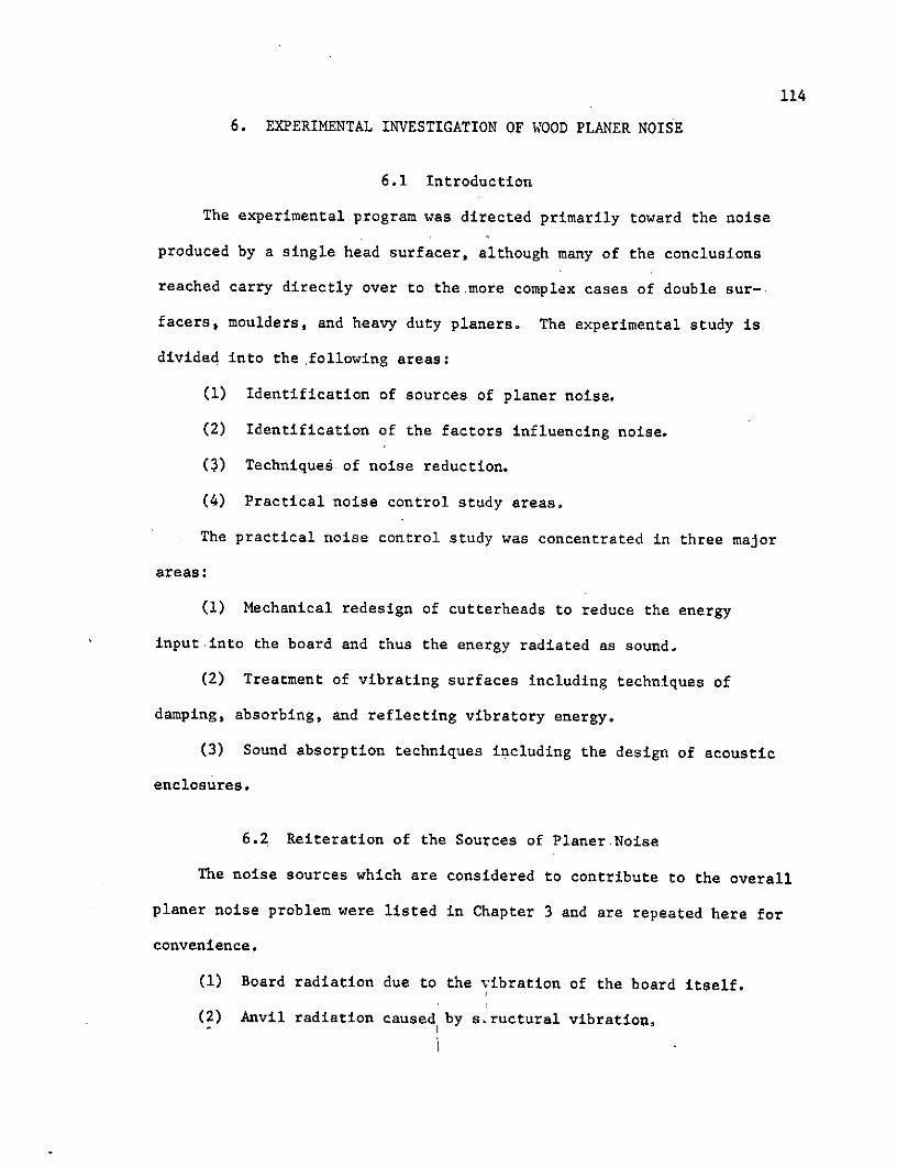
6.10 Sound Pressure and Acceleration Levels for Operationwith the Pressure Bar in the "Tight" and "Loose"Positions ............ . . . . . . . . . . . . 132
6.11 Comparison of Sound Pressure Level for Operation withand without the Chipbreaker . . . . . . . . . . . . . . . . 134
6,12 Acceleration Spectrum for the Chipbreaker Mechanism . . . . . 135
where the real part of the transfer impedance H (w) has been -taken.n
The solution is observed to contain only harmonic components at each
of the forced frequencies (w). The free vibration components, in the
presence of damping, decrease rapidly with time and for practical
purposes disappear. The term sin(nnx/z) is the expected sinusoidal
spatial variation in the response, and sin(nx o/9)represents a sup-
pression of frequencies in accord with the location of the force on
the beam. The forced vibration is observed to occur at the forced
frequency and harmonics with the amplitude being governed by the damp-
ing term (6i) in the vicinity of resonance (w=w ).
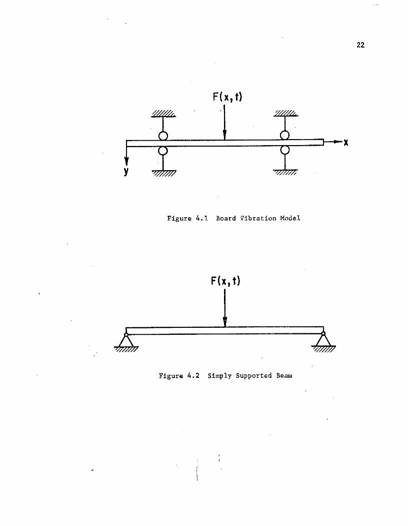
4.5 Application to Wood Planers
In the planing operation the bea;n represents the board being sur-
faced and the harmonic exciting force F(x,t) symbolizes the periodic
41
impact of the cutting knives on the board. The special case of a
square knife cutterhead arrangement can be represented with regard to
frequency by a fundamental blade passage frequency and harmonics of
this frequency, The contributing frequencies are given by
fh = BPF times n (Hz) (4.51)
where BPF is the blade passage frequency and n = 1,2,3...
The blade passage frequency is related to the cutterhead RPM and the
number of knives by
BPF = (RPM)(N)/60 , (4.52)
where N is the number of knives on the cutterhead.
For any type of periodic impact of the blades on the board the
resulting pulse can be subdivided into a series of pure-tone signals
which are harmonically related, i.e., all frequencies are integral
multiples of the fundamental frequency. Thus for any type of blade
impact. (cutterhead design) that repeats itself regularly, equation
(4.35) is valid. For the case of aperiodic impact, which cannot be
subdivided into a set of harmonically related pure-tones, the response
can be described in terms of an infinitely large number of pure-tone
components of different frequencies spaced an infinitesimal distance
apart and with different amplitudes.
42
5. THEORETICAL DEVELOPMENT OF A MODEL FOR BOARD RADIATION
5.1 Introduction
The vibration analysis has given the response of the board as a
function of time (or frequency) and position on the board. This rep-
resentation is often difficult to use in conjunction with the approxi-
mate relations for radiated sound resulting from a vibrating surface.
For closely spaced harmonic components the vibration state of the
board can be represented by average properties valid strictly for a
reverberant vibrational field. Thus, information regarding the vibra-
tional field obtained from energy considerations or experiments takes
the place of the exact relations of Chapter .4.
In the formulation of a model for board radiation the phase cell
concept of structural vibration is utilized. In effect, the board is
considered to be composed of a finite number of radiating piston ele-
ments. The critical frequency, which governs the overall radiation of.
sound from the board, is utilized to divide the radiation problem into
three frequency ranges. Expressions for the radiated sound power are
derived for each frequency range using formulations for a rectangular
baffled piston. The baffled restriction is removed by using a theo-
retical analogy with a freely suspended disk.
The radiation characteristics of narrow and wide boards are
compared theoretically and the radiated power is computed numerically.
The computed sound power levels are then converted to average sound
pressure levels using the semireverberant substitution technique.
43
5.2 The Vibrational Field
The board radiation problem can be modeled by considering the
beam to be composed of a finite number of piston elements. The vibra-
tional field of the board is defined using energy principles in terms
of board geometry and energy delivered to the board. Using a simple
piston model to obtain the radiation characteristics and energy con-
siderations to define the velocity field, it is possible to predict
the acoustic power output of the vibrating board.
In order to properly dimension and locate the piston elements it
is necessary to specify the mode shapes (eigenfunctions) and natural
frequencies (eigenfrequencies) of the vibrational field. In this
'analysis the response of the board is assumed to be reverberant in
nature; the individual modes being uncoupled and separated in fre-
quency, This is equivalent to assuming an input force consisting of
well spaced pure-tone frequency components with the frequency response
of the board concentrated in narrow frequency bands.
5.2.1 The Structural Wavelength
Above the first few natural modes the natural frequencies are
relatively independent of the particular type of boundary constraints.
The transverse structural wavelength for a uniform, rectangular,
slender beam is given by [3] as
n B [ci/pb 21/4 )/2V_ 1/514
ns f wn)1 /2 /2 6 (5.1)
44
where
Xns = modal structural wavelength of the nth mode,
CB = transverse bending.wave velocity,
f = n/21 .
Using equation (4.1) for the natural frequencies of such a beam, i.e.
2 EIg 1/2Wn = (/) 2 p j P (5.2)
in equation (5.1) above, yields
Xns = 2T /B (5,3)
The factor 8 depends on the particular mode, which in turn, depends on
the length of the beam. Equation (5.1) indicates that the modal struc-
tural wavelength (X ns) at a particular resonant frequency is dependent
only on the thickness and material constants of the beam, Although the
beam length governs the frequency corresponding to a particular mode,
the mode shape at a given frequency is independent of beam length.
Equation (5.1) is also independent of the boundary conditions. Figure.
5.1 shows the theoretical variation in wavelength with frequency as a
function of thickness and material, The reference frequency f is0
taken as the fundamental harmonic frequency in the Fourier spectra of
the excitation.
45
100-
SI 0
10 100f/f0
Figure 5.1 Structural Wavelength Parameter
Versus Fundamental Frequency
Ratio
46
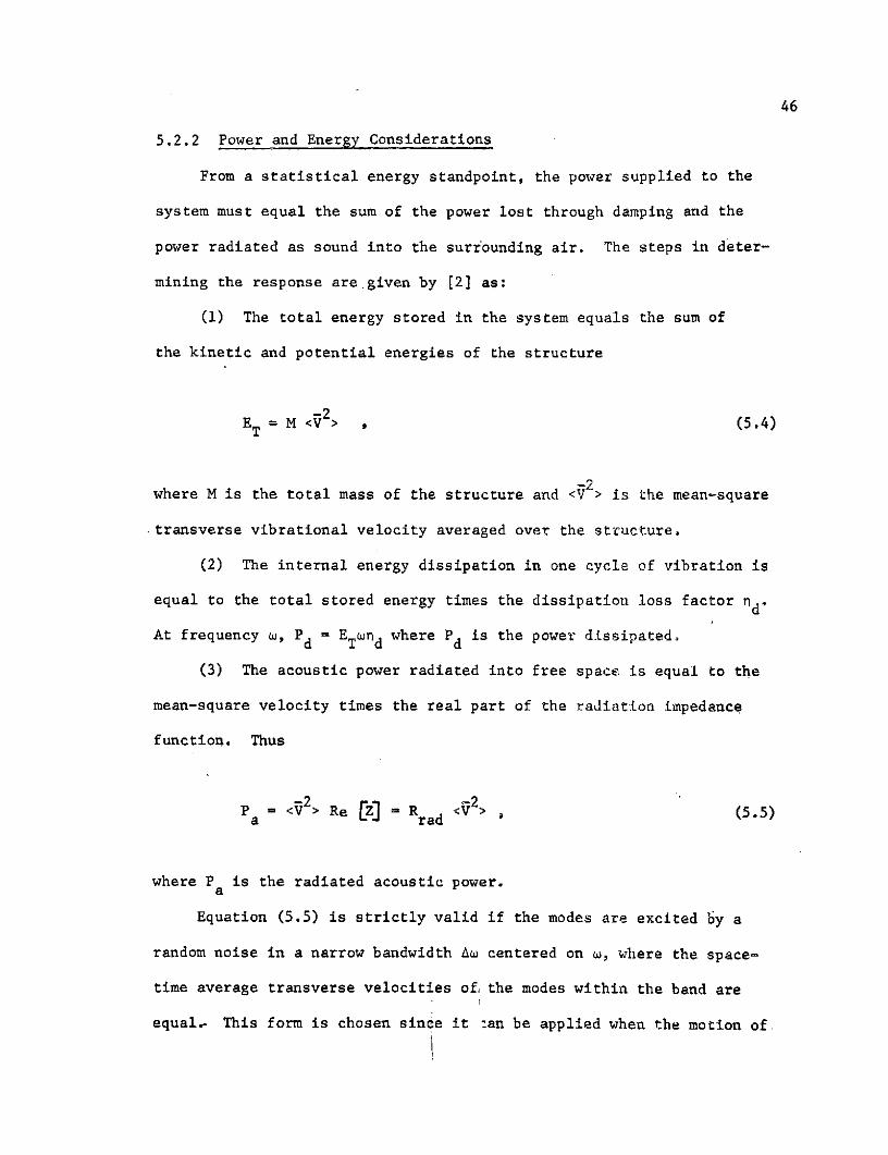
5.2.2 Power and Energy Considerations
From a statistical energy standpoint, the power supplied to the
system must equal the sum of the power lost through damping and the
power radiated as sound into the surrounding air. The steps in deter-
mining the response are given by [2] as:
(1) The total energy stored in the system equals the sum of
the kinetic and potential energies of the structure
ET = M <2> , (5.4)
where M is the total mass of the structure and <V2> is the mean-square
transverse vibrational velocity averaged over the structure.
(2) The internal energy dissipation in one cycle of vibration is
equal to the total stored energy times the dissipation loss factor nd '
At frequency w, Pd = ETWnd where Pd is the power dissipated.
(3) The acoustic power radiated into free space is equal to the
mean-square velocity times the real part of the radiation impedance
function. Thus
Pa = <2 > Re [Z] = Rrad <2> (5.5)
a rad
where Pa is the radiated acoustic power.
Equation (5.5) is strictly valid if the modes are excited by a
random noise in a narrow bandwidth Aw centered on w, where the space-
time average transverse velocities of, the modes within the band are
equal This form is chosen since it :an be applied when the motion of,
47
the structure is either single mode vibration or a reverberant vibra-
tional field. From equation (5.5) the radiation resistance is defined
as
Rra d = Pa/<v 2> (5.6)
In this case the radiation resistance is independent of the modal
energy of the structure. This is equivalent to assuming that the
mechanical resistance and the acoustic resistance achieve values inde-
pendently of the energy distribution; that is the modes are not coupled.
Using equation (5.4) relating energy, velocity, and mass, gives
<V2> = E /M . (5.7)
For a beam excited across its entire width (W) by a force (F) per
unit width, the energy input varies with width as
ET " W or ET/W = constant . (5.8)
Since the energy input is linearly related to the width, equation
(5.7) can be written as
-v2> = ET/(bWtb ) (5.9)<V > = ET/(pbWtbt) . (5.9)
48
where
M = PbWtb Z,
Pb = density of the beam,
W = width of the beam,
tb = thickness of the beam,
A = length of the beam.
combining equations (5.8) and (5.9) yields
<V2> = (ET/W) (1/btb)) 1/ (5.10)
for a given density and thickness. The velocity term is observed to be
independent of beam width since more energy is delivered for the wider
beam, thereby rendering the quantity ET/W constant. Equation (5.10)
states that the product of mean-square velocity and board length is
constanti a result which will be quite useful in obtaining the total
radiated sound power from the beam.
5.3 The Elementary Piston Model for Board Radiation
The present analysis is based on the replacement of the vibrational
field of the beam by an array of rectangular piston radiators, having
the characteristics of monopole radiators insofar as general behavior
is concerned. The phases of the monopoles correspond to the phase of
the vibrational field at each position. Each radiator (piston) has the
dimensions of d (one-half the structuoral wavelength, A /2) and W (the
width of the piston) and vibrates out of phase with a neighboring piston.
49
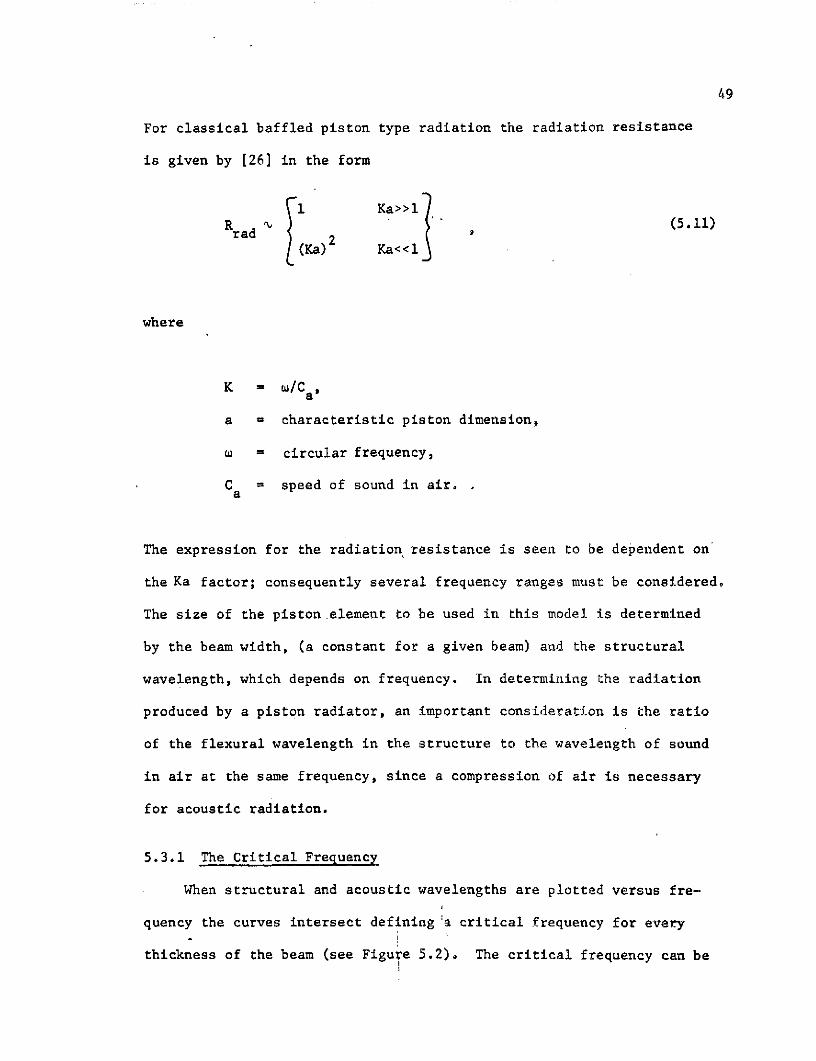
For classical baffled piston type radiation the radiation resistance
is given by [26] in the form
1 Ka>>lRrad 2 " (5.11)rad 2
(Ka) Ka<<1
where
K = w/Ca,
a = characteristic piston dimension,
w = circular frequency,
Ca = speed of sound in air.
The expression for the radiation resistance is seen to be dependent on
the Ka factor; consequently several frequency ranges must be considered,
The size of the piston.element to be used in this model is determined
by the beam width, (a constant for a given beam) and the structural
wavelength, which depends on frequency. In determining the radiation
produced by a piston radiator, an important consideration is the ratio
of the flexural wavelength in the structure to the wavelength of sound
in air at the same frequency, since a compression of air is necessary
for acoustic radiation.
5.3.1 The Critical Frequency
When structural and acoustic wavelengths are plotted versus fre-
quency the curves intersect defining a critical frequency for every
thickness of the beam (see Figure 5.2). The critical frequency can be
50
10.0
Sa
S1.0
CRITICAL FREQUENCY
0.1 1.0 10.0f/fc
Figure 5.2 Structural and Acoustic Wavelength
Versus Critical Frequency Ratio
51
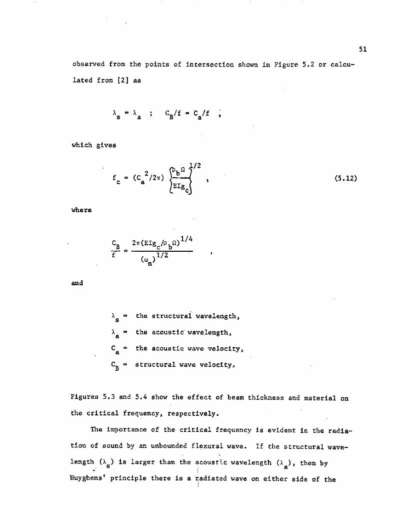
observed from the points of intersection shown in Figure 5.2 or calcu-
lated from [2] as
X = X ; C/f = C /f
s a B a
which gives
f = (Ca2/27) 2 (5.12)
where
C B 2 (EIg/P b) 1 / 4
f 1/2
and
X = the structural wavelength,
X = the acoustic wavelength,a
Ca = the acoustic wave velocity,
CB = structural wave velocity,
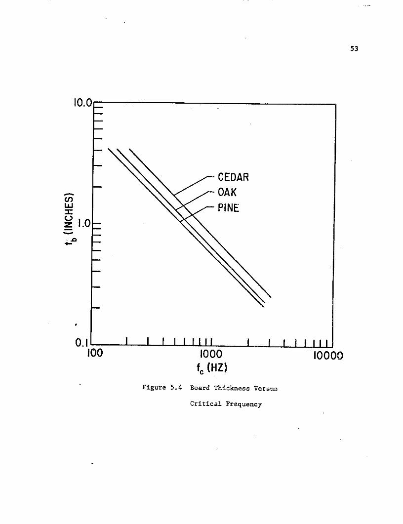
Figures 5.3 and 5.4 show the effect of beam thickness and material on
the critical frequency, respectively.
The importance of the critical frequency is evident in the radia-
tion of sound by an unbounded flexural wave. If the structural wave-
length (X s) is larger than the acoust tc wavelength (X ), then byHuyghens principle there is a radiated wave on either side of theHuyghens' principle there is a radiated wave on either side of the
52
100
tb
Stt II
b2
_ \x
*CRITICAL FREQUENCY
IoI I Iooo I I I Io ooo100 1000 10000
f(HZ)
Figure 5.3 Acoustic and Structural
Wavelength Versus Frequency
53
10.0
CEDAR
OAKC-... I PINEz 1.0
1.0
o 1 1 111I Io II Ii100 1000 10000
fc (HZ)Figure 5.4 Board Thickness Versus
Critical Frequency
54
structure forming the angle 6 = sin-l1 ( a s) between the direction of
propagation and the normal to the structure. As XA approaches a the
angle moves toward its maximum. If Xa surpasses hs then 6 becomes
imaginary and radiation fails. In effect the contrary motions of
adjacent portions of the structure cancel, resulting in zero radiation.
For a finite beam, interior sections effectively cancel each other
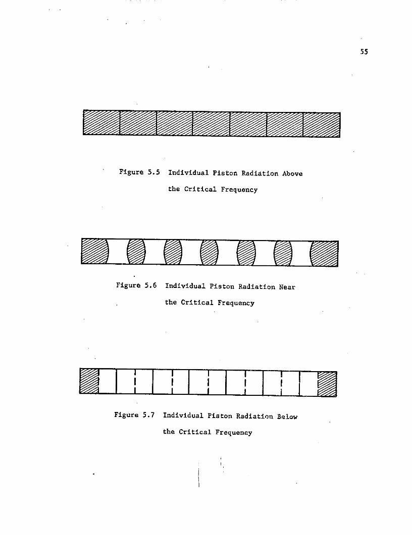
leaving only the end portions as radiators. Three cases of radiation
are considered according to the ratio of A to A , which defines thea s
amount of interference between neighboring pistons, This is equivalent
to dividing the radiation problem into three frequency ranges, being;
above the critical frequency (As > a ), at or near the critical fre-
quency (Xs A ), and below the critical frequency (A< a a)' The three
cases can be represented diagramatically, with the shaded areas being
the radiating acoustic sources in Figures 5.5, 5.6, and 5.7. Above the
critical frequency (As > a ) the phase cells of Figure 5.5 are decoupled
and cancellation effects are negligible. At or near the critical fre-
quency (As = Xa) the cells.are coupled but internal cancellation is
incomplete. The radiating area, the shaded portion of Figure 5.6, is
a fraction of that for the case above the critical frequency. Below
the critical frequency (As < a ) the phase cells, acting as point
monopoles localized at the cell center, interfere and internal cancel-
lation is complete. Only the edge monopoles of Figure 5.7 of half
strength are left as radiators. The three cases considered correspond
to Ka> 1, Ka\l, and Ka< 1, respectively, with "a" being a typical
piston (phase cell) dimension.
55
Figure 5.5 Individual Piston Radiation Above
the Critical Frequency
Figure 5.6 Individual Piston Radiation Near
the Critical Frequency
Figure 5.7 Individual Piston Radiation Below
the Critical Frequency
56
5.3.2 The Phase Cell Concept
The phase cell concept is used to represent the instantaneous
relative phase of neighboring piston elements constituting the beam.
The length of each piston is determined by the structural wavelength
of the beam at a particular frequency. For example, the pure-tone
component shown in Figure 5.8 would be represented by the phase cell
arrangement of Figure 5.9. In Figure 5.9 the length of each piston
element is d = X /2; one-half the structural wavelength.s
For the case of a beam mounted in an infinite plane baffle the
radiation can be characterized by an array of rectangular baffled
pistons, with each piston affecting a neighboring piston in accord
with the three frequency ranges discussed. The model must be altered,
however, to allow for a beam radiating into free space. In analogy
with the freely suspended disk of [24], the unbaffled piston elements
behave in much the same manner as the baffled piston for cases such
that Kb >1, where b is one-half the vector distance between the
monopole sources located on each piston face. For values of Kb such
that Kb <1 the monopole sources on each face of the piston exhibit
cancellation effects similar to the case of X < X for neighborings a
piston elements. The total radiation of the beam is composed of the
contribution of N piston elements, where N is determined by the beam
length, structural wavelength, and Ka factor for the particular fre-
quency of interest.
5.4 Acoustic Power Radiation
Utilizing the phase cell model, 'the radiation resistance can be
approximated in each frequency domain as a function of the various beam
57
Figure 5.8 Structural Wavelength Illustration
-I + i +1
Figure 5.9 Phase Cell Representation of
Structural Wavelength
58
parameters. The total acoustic power (Pa) radiated to the far field
is given by [2] as
P = R <2> (5.13)a rad
The quantity <V2> is the mean-square (space-time averaged) transverse
velocity of the beam (or piston element), This velocity may be obtained
theoretically using the methods of Chapter 4, or approximated by means
of the energy techniques discussed elsewhere in this section. It has
been shown, (see equation (5.9)), that the quantity <V2> for a rever-
berant vibrational field may be expressed in terms of the beam mass and
the energy input to the system. The mean-square velocity was observed
to decrease with increasing beam length for a constant energy input, as
expected from the concept of equipartition of energy for reverberant
systems. Repeating equation (5,10)
<-2> = ET/(pbtbaW) " 1/z . (5.14)
The quantity ET is the energy stored in the beam and is independent of
the length of the beam. From equation (5.14) it is observed that for
a particular beam the product < 2> 2 is constant and the resulting
acoustic power output of the beam can be expressed from equation (5.13)
as
Pa = (Rrad)( <V2>) conspant*(R ad/) , (5.15)a a d'.
59
Thus, the task is reduced to determining the radiation resistance for
the different frequency domains and beam geometries.
5.4.1 Individual Piston Behavior
The piston model formulation is general (valid for all values of
Ka) for each individual piston, but the number of radiating pistons
(N p) will depend on the particular frequency with respect to the criti-
cal frequency. Preliminary to determining the values of the radiation
resistance, it is necessary to examine a single unbaffled piston in
detail to determine the combined behavior of monopole sources located
on each face. This is equivalent to considering a dipole source of
strength Qb for Kb<l, where Q is the equivalent simple source strength.
Thus, the model accounts for short circuiting at low values of Kb for
the unbaffled beam.
Figure 5.10 shows a section through the beam along with an indi-
vidual piston element. In the equivalent source model of Figure 5.11,
the monopole sources are considered to be concentrated at the piston
centers, reversed in phase. For the two sources of Figure 5.11 to
form an effective dipole, it is required that b < Xa/2. In analogy
with the freely suspended disk of [24], the radiation resistance can
be represented by
(2pc)irr for Kr>>l
Rrad = ; (5.16)
(3pc)(Kr) 4r2 for Kr<<l
where pc is the specific acoustic impedance and r is the disk radius.
60
I-C- s/2
xs/2
Figure 5.10 Individual Piston Element
e-I1
Figure 5.11 Simple Source Model for
Piston Radiation
61
For values of Kr>l the baffled and unbaffled piston radiation differs
by a factor of two, accounting for radiation from both sides for the
latter case. The radiation is altered only in the range of Kr<l. In
this region (Kr<l) the following expressions for the radiation resis-
tance are appropriate
pcA(Kr)2/2 (baffled)
Rrad = 0 (5.17)
3pcA(Kr) (unbaffled)
for Kr<l.
The radiation efficiency, defined as radiation resistance divided
by pcA, takes the form
Rrad r (Kr)2/2 (baffled)
a = pcA , (5.18)
3(Kr)4 (unbaffled)
for Kr<l.
Thus the radiation efficiency for the baffled piston is greater than
that for the unbaffled piston for small Kr, (Kr<l). The value of Kr
where the curves of a versus Kr intersect for the two cases is found
from equation (5.17) as
(Kr) 2/2 = 3(Kr) or Kr = //6 . (5.19)
62
Short circuiting is possible for values of Kr<l6; for values of
Kr>l/6 the radiation for the baffled and unbaffled pistons differ only
by a factor of two. Figure 5.12 indicates the difference in the radia-
tion characteristics for the two casds for Kr<l/6, For a typical piston
dimension "a" (a = 2r) it is assumed for Ka<l short circuiting effects
are possible and for Ka>l they are not possible.
The radiation field for a flat, rectangular piston set in a plane
rigid wall is considered; the far field relations for the radiation
impedance being deduced from the well known case of the baffled circu-
lar piston. As indicated, the deviation of the unbaffled beam from the
baffled case due to cancellation is apparent only for values of Ka such
that Ka<l, where "a" represents an effective diameter,
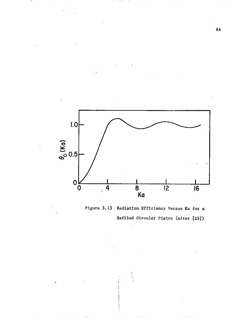
In accord with [24] for a baffled circular piston
Rra d = pcA 8 (Ka) (5.20)
where
eo(Ka) = [1-(2/Ka)J 1 (Ka)]
and J1 is the Bessel function of order one. The function e (Ka) is
plotted versus Ka in Figure 5.13.
In converting from the baffled circular piston to the baffied
rectangular piston the approximate result given in (24] is
[a e0 (Ka) - b2 e(Kb)Rrad= pcA[2 _ b 2 - (5.21)
63
10I
Ka = 2Kr I
8- /
26- /
4 - BAFFLEDPISTON /
2- /
'Ie // UNBAFFLEDPISTON
0 1 -I i0 0.2 0.4 0.6 0.8 1.0
Ka
Figure 5.12 Radiation Efficiency for Baffled
and Unbaffled Pistons at Low Ka
64
1.0
,o0.5
0 4 8 12 16Ka
Figure 5.13 Radiation Efficiency Versus Ka for a
Baffled Circular Piston (after [15])
65
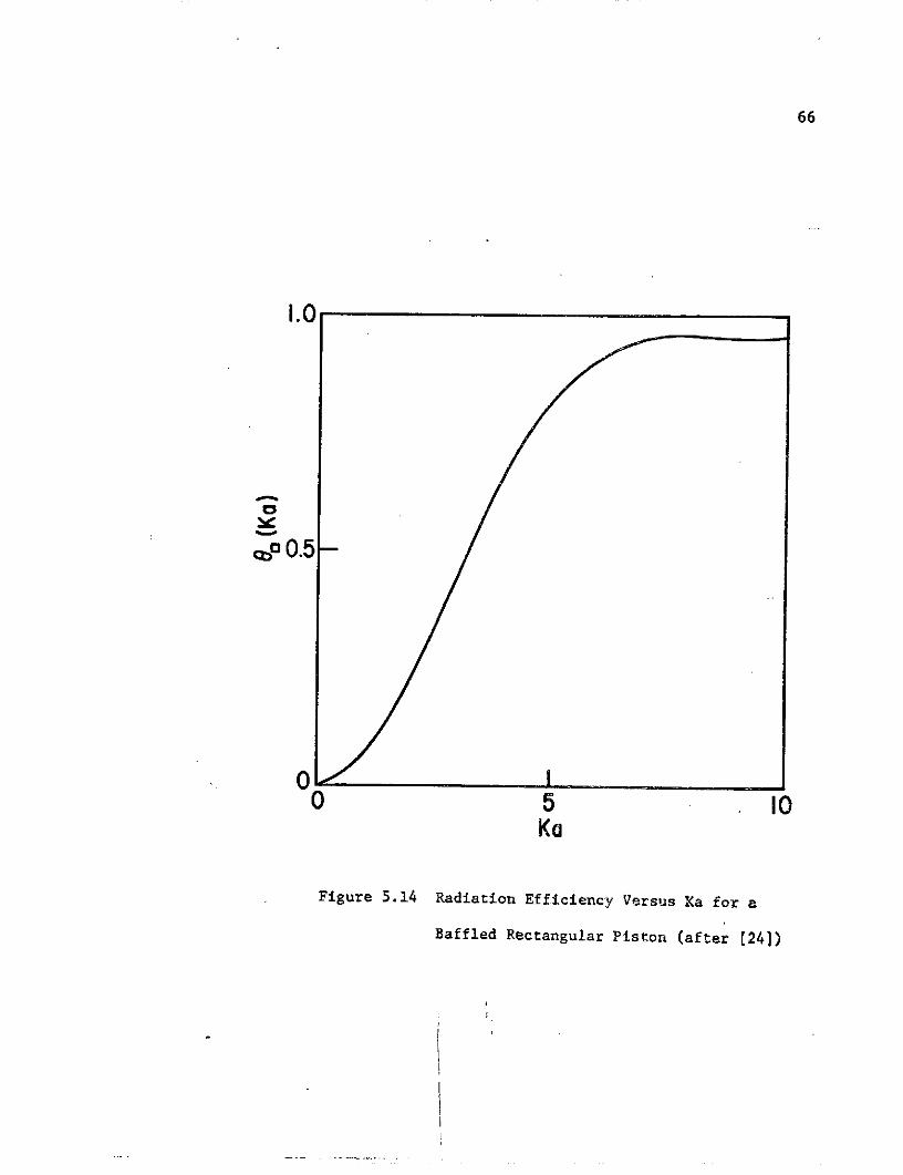
where
1-J (Ka)80 (Ka) = 1-42 (5.22)
and the piston area (A) = ab, with Jo the Bessel function of zero
order. Figure 5.14 indicates the variation of e with Ka for a
rectangular piston.
For the special case of a square baffled piston the radiation resis-
tance formula reduces to
Rra d = pcA e (Ka) , (5.23)
where eo is defined by equation (5.20). The function 60 (Ka) exhibits
the following properties;
e (Ka) 1 1 ; Ka>4
O (Ka) ' Ka ; 2<Ka<4 (5.24)
a (Ka) ' (Ka) ; Ka<2
Combining equations (5.24) and 5.23) gives
pcA ; Ka>4
Rrad ' pcA(Ka) ; 2<Ka<4 (5.25)
pcK2A2 ; Ka<2
66
I.0
QJ0.5
0 I0 5 .10
Ka
Figure 5.14 Radiation Efficiency Versus Xa for a
Baffled Rectangular Piston (after (241)
67
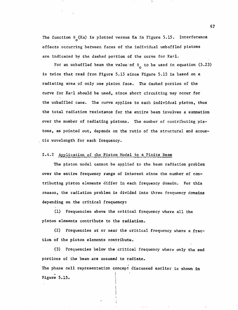
The function o0 (Ka) is plotted versus Ka in Figure 5.15. Interference
effects occurring between faces of the individual unbaffled pistons
are indicated by the dashed portion of the curve for Ka<l.
For an unbaffled beam the value of 0o to be used in equation (5.23)
is twice that read from Figure 5.15 since Figure 5.15 is based on a
radiating area of only one piston face. The dashed portion of the
curve for Ka<l should be used, since short circuiting may occur for
the unbaffled case. The curve applies to each individual piston, thus
the total radiation resistance for the entire beam involves a summation
over the number of radiating pistons. The number of contributing pis-
tons, as pointed out, depends on the ratio of the structural and acous-
tic wavelength for each frequency.
5.4.2 Application of the Piston Model to a Finite Beam
The piston model cannot be applied to the beam radiation problem
over the entire frequency range of interest since the number of con-
tributing piston elements differ in each frequency domain. For this
reason, the radiation problem is divided into three frequency domains
depending on the critical frequency:
(1) Frequencies above the critical frequency where all the
piston elements contribute to the radiation.
(2) Frequencies at or near the critical frequency where a frac-
tion of the piston elements contribute,
(3) Frequencies below the critical frequency where only the end
portions of the beam are assumed to radiate.
The phase cell representation concept discussed earlier is shown in
Figure 5.15.
68
1.2
1.0-
0.8
0.6CP
0.4
0.2
0 2 4 6 8 10Ko
Figure 5.15 Radiation Efficiency Parameter Versus Ka
for Baffled and Unbaffled Pistons
69
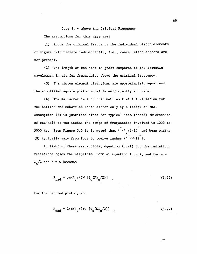
Case 1. - Above the Critical Frequency
The assumptions for this case are:
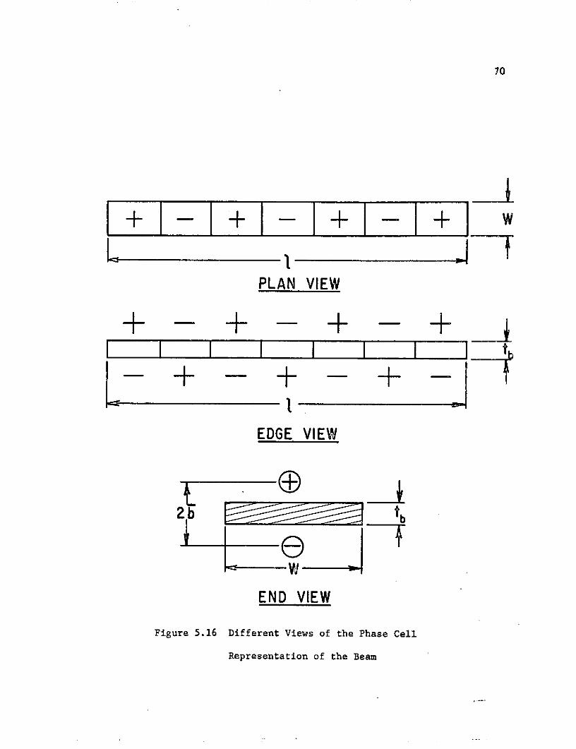
(1) Above the critical frequency the individual piston elements
of Figure 5.16 radiate independently, i.e., cancellation effects are
not present.
(2) The length of the beam is great compared to the acoustic
wavelength in air for frequencies above the critical frequency.
(3) The piston element dimensions are approximately equal and
the simplified square piston model is sufficiently accurate.
(4) The Ka factor is such that Ka>l so that the radiation for
the baffled and unbaffled cases differ only by a factor of two,
Assumption (3) is justified since for typical beam (board) thicknesses
of one-half to two inches the range of frequencies involved is 1000 toII I
5000 Hz. From Figure 5.3 it is noted that 4 <X s/2<10 and beam widths
(W) typically vary from four to twelve inches (4 <W<12 ).
In light of these assumptions, equation (5.21) for the radiation
resistance takes the simplified form of equation (5.23), and for a =
X /2 and b = W becomes
Rra d = pc(Xs/2)W [e o(KX /2)] (5.26)
for the baffled piston, and
Rra d = 2pc( s/2)W [e (Ks /2)] , (5.27)
70
+-I I+ - + 1+ w
PLAN VIEW
-- + -+ -+
EDGE VIEW
2b tbL -LeEND VIEW
Figure 5.16 Different Views of the Phase Cell
Representation of the Beam
71
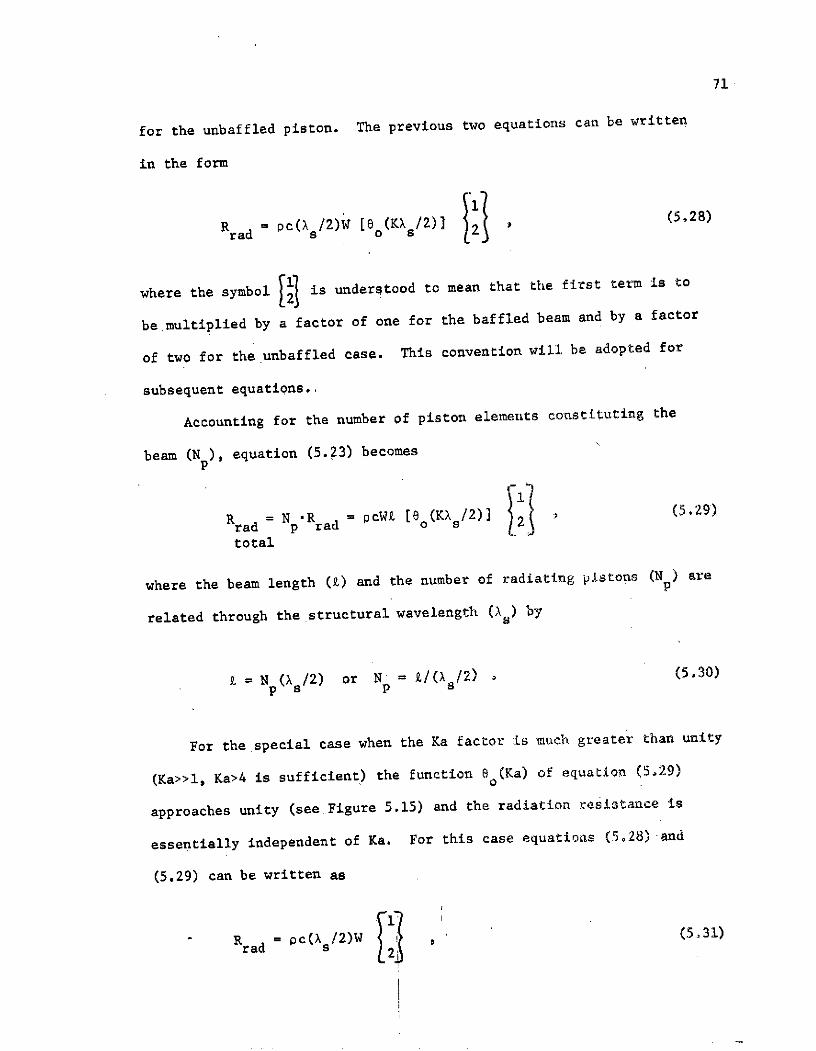
for the unbaffled piston. The previous two equations can be written
in the form
rad = pc(X /2)W [e (KX /2) 2 (5.28)
where the symbol is understood to mean that the first term is to
be.multiplied by a factor of one for the baffled beam and by a factor
of two for the unbaffled case. This convention will be adopted for
subsequent equations.
Accounting for the number of piston elements constituting the
beam (N p), equation (5.23) becomes
rad = N *Rad = pCW [6 0 (KX /2)] 2 (5,29)
total
where the beam length (Z) and the number of radiating pistons (N p) are
related through the structural wavelength (X,) by
z = N p( /2) or N = 9/(X /2) - (5.30)
For the special case when the Ka factor is much greater than unity
(Ka>>l, Ka>4 is sufficient) the function eo(Ka) of equation (5.29)
approaches unity (see Figure 5.15) and the radiation resistance is
essentially independent of Ka. For this case equations (5.28) and
(5.29) can be written as
Rrad = pc(As/2)W (5.31)
72
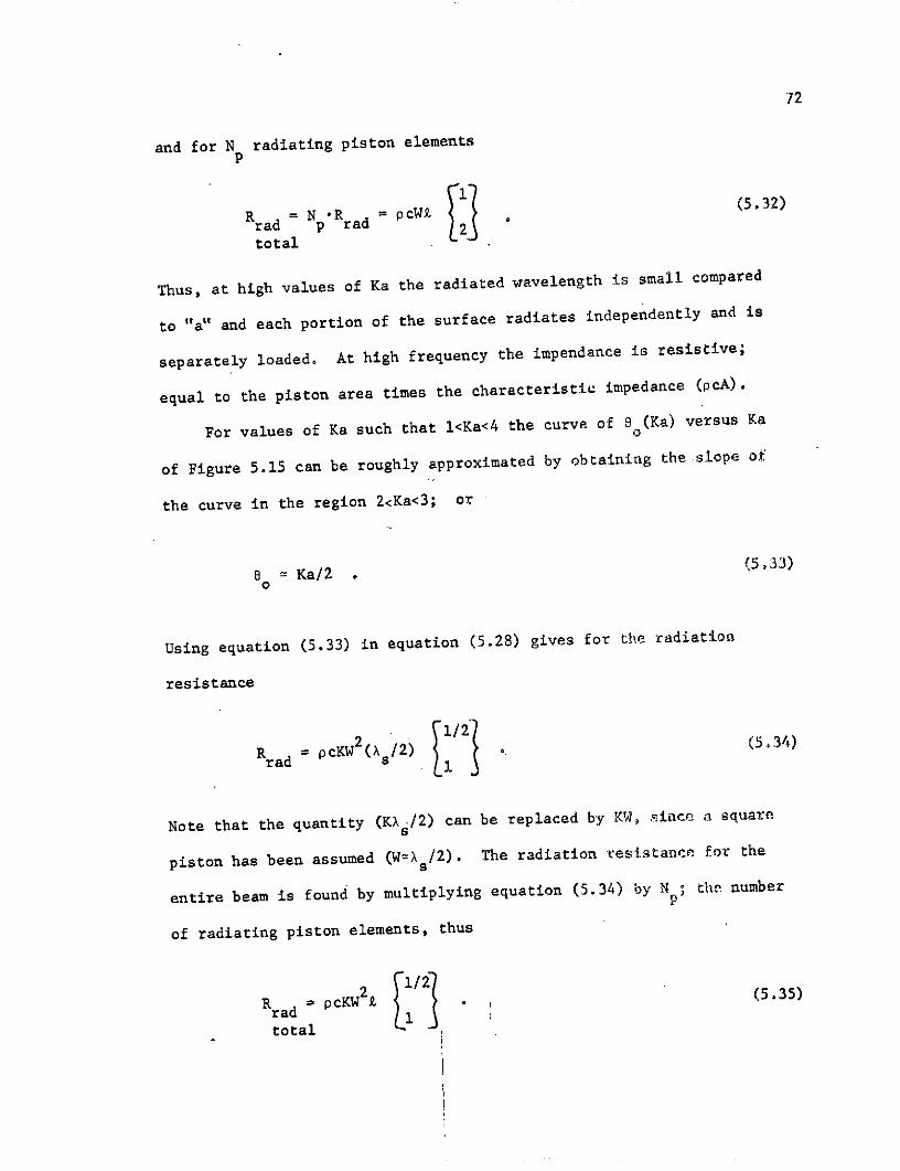
and for N radiating piston elements
R rad= N R a= PCWZ (5.32)
total
Thus, at high values of Ka the radiated wavelength is small compared
to "a" and each portion of the surface radiates independently and is
separately loaded. At high frequency the impendance is resistive;
equal to the piston area times the characteristic impedance (pcA).
For values of Ka such that 1<Ka<4 the curve of 9 (Ka) versus Ka
of Figure 5.15 can be roughly approximated by obtaining the slope of
the curve in the region 2<Ka<3; or
0 = Ka/2 (5,33)
o
Using equation (5.33) in equation (5.28) gives for the radiation
resistance
Rrad = pcKW2 (X /2) /2 (5.34)
Note that the quantity (KXs/2) can be replaced by KW, since a square
piston has been assumed (W=X s/2). The radiation resistance for the
entire beam is found by multiplying equation (5.34) by N ; the number
of radiating piston elements, thus
2 9 1 / 2 1R r pcKW (5.35)
rad Itotal
73
The results obtained for the baffled beam can be compared with
the results obtained in [21] and [22]. Defining the surface area S
(S = Wk) the radiation resistance for the baffled case, as given by
equations (5.32) and (5.35), is
pcS ; KW4
Rrad = (5.36)
total 1pcKWS ; 1<KW<4
For frequencies above the critical frequency such that A >A and
t>X a, [21] gives the radiation resistance as
Rrad = pcS(l-(a /s) 2 ) 1/ 2 cS , (5.37)
where y<1 (high Ka) and y is taken as - KW(l-(A s)2) 1 / 2
For y<l, the radiation resistance is given as
R = 1 SpcKW (5.38)rad 2SPc
which is also the result obtained in (22] for a narrow beam,
Case 2. - Near the Critical Frequency
The assumptions for this case are:
(1) At or near the critical frequency the piston elements of
Figure 5.16 do not radiate independently. The radiation from one
phase cell partially cancels that from adjacent cells since they are
180 degrees out of phase. The degree of cancellation ranges from
74
zero, slightly above the critical frequency, to unity below the criti-
cal frequency.
(2) The beam is long compared to the acoustic wavelength
(Z>Xa/2).
(3) The KS factor is such that Kb>1 so that the faces of an
individual piston element radiate independently.
(4) The assumption made on the fraction of cancellation over-
powers the magnitude of the errors involved in assuming that Xs/2=W
in this frequency range, so that the square piston model is again
assumed.
In regard to assumption (1), the exact degree of cancellation between
neighboring phase cells in the vicinity of the critical frequency is
unknown. In this narrow frequency range the cancellation, theoreti-
cally, jumps from zero to unity. To account for this effect an
average amount of cancellation of one-half can be assumed without
great inaccuracies, which is essentially what is done in [21], As-
sumption (3) is justified since for midrange values of Ka(1/2<Ka<4)
the two faces of an individual phase cell radiate as independent mono-
poles.
Assuming that neighboring pistons, spaced one-half of a struc--
tural wavelength apart, partially cancel resulting in an effective
decrease in the number of radiating piston elements by a factor of one-
half, the expression for the radiation resistance for the square piston
model is
rad= N rad cWoe KX /2) (5.39)rad p rad 2total
75
where
Rrad = pc(Xs /2)W 6 (KX s/2) (5.40)
and N = 1/2 [i/s /2] since effectively only half of the pistons
contribute.
The more accurate expression for the rectangular piston model
given by equation (5.21) is
S (X/2) 2 o (KX /2) - W2 (KW)R = N R pcW1 [ s s (5.41)
radtotal p rad 2 ((Xs/2) 2_W2)
Several special approximations depending on the Ka factor are presented.
Ka factor less than unity (Ka<l), The function 0 for the baffled and
unbaffled piston elements is approximated by
(Ka)2/2 (baffled)
8 % (5,42)
o 3(Ka)4 (unbaffled)
so that
(KX /2)2/2
Rrad =f pC(s/2)W (543)
6(KX /2) 4
S
76
and
(KX /2) 2/2
R =N R cW1 (5.44)rad p rad 2total 6(KX s/2) 4
Ka factor ranging from one to four (l<Ka<4), In this region the curve
of Figure 5.15 is approximated by
80 = Ka/2 = (KX /2)/2 = KW/2 , (5.45)
so that
R = pcKW2 ( s/2) (5,46)rad s
and
1/2R = N R i pcKW2 (5,47)rad p rad 2total
Ka factor greater than four (Ka>4), In this Ka region the function
o(Ka) becomes independent of Ka and approaches unity
S= 1 (5,48)
77
so that
Rrad = pc(Xs/2)W [2 (5.49)
and
R =N.RR rad = 1 pcWL (5.50)rad p rad 2 PCWtotal
Since the square piston model has been assumed, the terms (X /2) and
W have been used interchangeably.
In summary, the following approximate results are obtained for the
radiation resistance for several ranges of Ka for frequencies near the
critical beam frequency.
pcWR(KW)2 ; KW<13(KW)2
2 1/4Rd = pcW2£K 1; <KW<4 (5,51)
total
pcWi ; KW>4
The result obtained in equation (5.51) for 1<Ka<4 may be compared
with that of [21] for the baffled beam which also gives
R 1 pcKW2 . (5.52)rad 4 .
78
Case 3. - Below the Critical Frequency
Below the critical frequency the mode shape of the beam fn(x) is
such that the structural wavelength is very short compared to the
acoustic wavelength. Thus the radiation from a crest to a node segment,
shown in Figure 5.17, is effectively cancelled by the radiation from
the adjacent segment, which is 180 degrees out of phase. By extending
this argument, it is concluded that all the radiation from the central
portion is effectively cancelled, so that the radiation must be
accounted for by the end segments of length ( s/4). The radiation is
equivalent to the.coupling of a pair of rigid pistons, each having a
mean-square velocity equal to the mean-square velocity of the whole
beam and vibrating with the same relative phase as the end regions of
the beam.
Below the critical frequency the faces of individual piston ele-
ments may act as monopoles radiating independently or, for the un-
baffled case, a higher order source (dipole) depending on the frequency
and piston geometry. As discussed earlier, the baffled and unbaffled
pistons differ by a factor of two for Ka>l, since the effective radi-
ating area is doubled., For Ka<1 short circuiting may occur between
the two radiating faces of the piston for the unbaffled case. This
leads to lower values of the radiation resistance than the values for
a completely baffled piston. The short circuiting ((Ka) term) effect
is shown in Figure 5.12 along with the baffled piston curve ((KA)2
term) for low values of Ka. The simplified model for the square piston
element is assumed since in this frequency range the piston (beam)
width-is approximately equal to the iuantity (~ /4), If the width (W)
79
is such that 4 <W<12 and the frequency range under consideration
satisfies the relationship 100<f<1000 (Hz), then from Figure 5.2
5 <X /4<12 so that the square piston model assumption is again
justified.
In Figure 5.12 (Ka)4 and (Ka)2 like terms were plotted versus Ka
up to the point of intersection of the two curves. The dipole effect
of the piston faces is present only for such Ka that the term 3(Ka)4
is less than (Ka)2/2 since the dipole cannot surpass the monopole in
efficiency. The radiation resistance relations are again based on the
square piston model, but in the frequency range below the critical fre-
quency the model cannot be applied without certain restrictions con-
cerning Ka and the beam length. The size of the end piston elements
which radiate is now (Xs/4>(W), as shown in Figure 5.18.
Several special cases of beam radiation below the critical fre-
quency will be considered.
Radiation from a long beam with (>X a/2>As/2 ; KW>1). This is
equivalent to assuming that the end pistons are sufficiently far apart
to radiate as independent monopoles and the individual pistons faces
radiate independently as if in a baffle. The expression for the radi-
ation resistance from equation (5.23) is
R = pcabs (a)
(5.53)
= pc(Xs /4)We0 (KXs 4)
80
Figure 5.17 Diagram of Beam Radiation Below
the Critical Frequency
Figure 5.18 Phase Cell Representation of Beam
Radiation Below the Critical Frequency
81
and since only two piston elements radiate (Np =.2)
Rrad = N rad = 2pc( /4)W [ (KX/4)] (5.54)
total
The function 0 (Ka) is again approximated for l<Ka<4 by
8 0 = Ka/2 = K(Xs /4)/2 (5.55)
and since the square piston model is assumed to be valid
0 = KW/2 . (5.56)
Combining equations (5.54), (5.55), and (5.56) and again noting that
only two piston elements radiate (Np=2) the radiation resistance for
the beam becomes
R = 2pcKW( /4)2 (5.57)rad stotal
for 1<Ka<4, where X /4 has been replaced by W, the piston width.
The results obtained can be compared with those of [21] which
gives
R 2 [2-(X /X) )2(W s s aR = aW (s) 2)3/ 2 (5.58)ra d pc X a [(1 s/ 2 a) 3/2
82
or
Rrad pcWK(Xs /4) 2 (5.59)
for the baffled piston since the acoustic wavelength is related to K
by Aa = 2r/K.
Radiation from a long beam with (£>Xa/2>Xs/2 ; KW<I). This is the
case of a beam, long compared to the acoustic wavelength (Xa), but
exhibiting dipole effects due to the interference between the faces of
each piston. Thus the baffled and unbaffled beam must be analyzed
separately. The function eo in this frequency range is noted from
Figure 5.15 to be
e0 (Ka)2/2 (baffled)
(5.60)
oa 3(Ka) 4 (unbaffled)
Using equation (5.23) for the square piston model, the radiation resis-
tance per piston becomes
Rra = P(X /4)W 0 (KX /4) (5.61)
83
Using equation (5.60) in (5.61) and accounting for two radiating
pistons gives
(KW) /2
R ra d = N .Rad 2pc(Xs/4)W , (5.62)
total 3(KW) 3
for Ka<l.
For the case of a baffled beam, [21] gives the radiation resis-
tance for X >X , 7T>a and W< asa s a a
Rra d pcW2 (KX /4) 2 (5.63)
which is in agreement with equation (5.62).
The remaining cases to be considered are beams which are not long
compared to the acoustic wavelength. This is not the usual case, since
in most practical situations the beam length (Z) is greater than three
feet (a machine operation requirement) and such low frequencies that
(3 <<X /2) are of little interest. For this case the edge monopoles
are coupled, and (a) the individual piston faces are uncoupled (Ka>l),
or (b) the value of Ka is less than unity and the faces are also coupled
(this is applicable to the unbaffled beam only).
There are two further cases to consider:
(1) The edge monopoles are in phase, and the interference is
constructive producing a total radiated power twice that if separated.
(2) The edge monopoles are oppos3ite in phase giving rise to a
dipole, radiating power that is second order to that of a monopole.
84
The resulting radiation may thus be characterized as monopole, dipole,
or quadrupole in nature depending on the relative phase of the end
portions and whether the beam is baffled or unbaffled.
The equations governing the radiation resistance in the three
frequency domains associated with the critical frequency are given in
Table 5.1 for baffled and unbaffled beams. The critical frequency to
be used in Table 5.1 for a particular beam geometry and material is
found from Figure 5.2.
5.4.3 An Exact Solution for Beam Radiation
The exact solution for the radiation from an infinitely long
cylindrical beam given by [24] has been generalized in (14] to apply
to beams of elliptic cross section and extended to include beams of
rectangular cross section. An outline of this analysis is presented,
subject to the following assumptions:
(1) The beam is infinite in extent, thus the radiation is
limited to frequencies above the critical frequency ( > a ).
(2) Coupling between normal modes of vibration due to damping
is neglected since the modes are well separated and in theory a uniform
damping force will not couple transverse vibratory modes,
(3) Internal damping is independent of frequency but does depend
on such factors as material, size, and moisture content and is speci-
fied experimentally.
(4) Air viscosity is neglected, reducing the problem to that of
acoustic radiation.
(5) The amplitude variation is -inusoidal and end effects are
neglected.
85
Table 5.1 Radiation Resistance for Different Values of the Ka Factor
for Each Frequency Range
Ka Factor Beam Length Piston " Frequency RadiationAssumption Dimensions Range Resistance
ALL* a > Xa/2 Xs/2 = W f > f pcW o( KW) I
KW>4 I >Xa/2 Xs/2 z W f> f' pcWM 2
K<W<4 a > Xa/2 Xs/2 W f > f 1/2pcW2gK 1
ALL* a > Xa/2 As/2 = W f = fc /2pcW£oe(KW)
K< W<4 a > Xa/2 Xs/2 z W f z f 1/4pcKW2 k
KW<l Z > Xa/2 Xs/2 z W f f pcWa (KW)2/4J
ALL* I > Xa/2 Xs/2 = W f < f pcW2 o(KW) [2
K<W<4 a > Xa/2 xs/2 = W f < fc pcW2 (W) 1
KW<1 a > Xa/2 Xs/2 : W f < f pcW2 (K)4
* For values of KW<1 the expression given for the radiation resistance
is valid provided the curve corresponding to the baffled or unbaffled
case in Figure (5.16) is used.
86
Finite beams vibrating in modes above the first few resonances usually
meet the above assumptions. Subject to these assumptions, [14] gives
the acoustic loss factor (na) as
na = -Re{FR /Vcos(Kx)e-it)} (1/(pbWtb)) , (5.64)
where
FR = beam radiation loading,
na = acoustic loss factor,
Re = real part of quantity,
b = mass density of the beam,
W = circular frequency,
W = beam width,
i =
tb = beam thickness,
t = real time,
vo = surface velocity.
The loading term FR is a quite complicated combination of Mathieu
functions and their derivatives for which expansions in terms of Bessel
and Hankel functions are required. The values of the loss factor (n a )
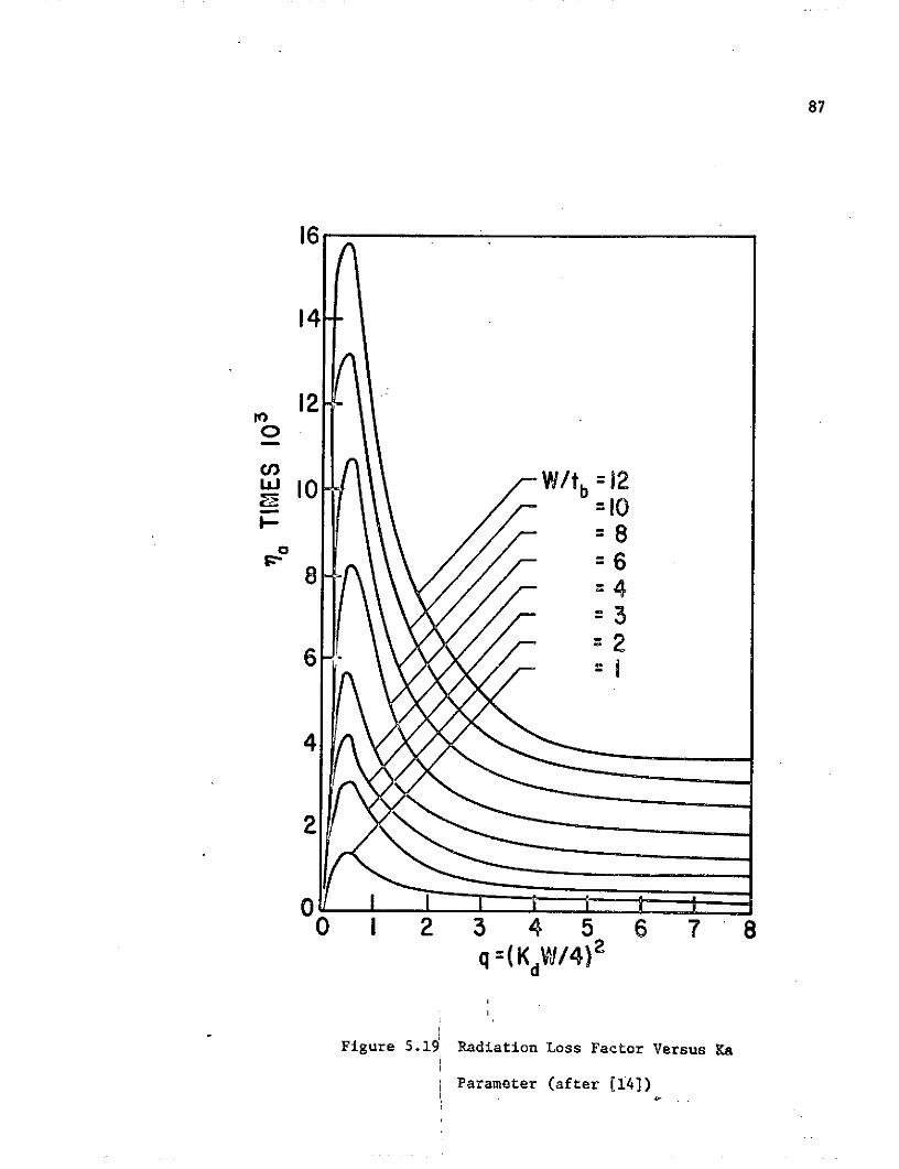
versus a dimensionless frequency parameter (q) are shown in Figure 5.19
for various beam width to thickness ratios. A plot of Kd given by1/2
[(2r/a ) -(2nr/X)2 ] versus frequency reveals that for the thicknessa s I
range of interest Kd is essentially iriependent of thickenss, making
87
16
14
12
10 b_ -' /b =2
8
8- -6=4=3=2
4
0
q =(KdW/4) 2
Figure 5.19 Radiation Loss Factor Versus Ka
Parameter (after (141)
88
it possible to plot na versus frequency for various beam widths. The
results, shown in Figure 5.20,are valid only above the critical fre-
quency for each particular thickness of the beam.
The relation between the radiation resistance (R rad ) and the loss
factor (na ) for finite beams is given by
Rrad = Mna , (5.65)
where w is the circular frequency and M is the total mass of the
structure.
At first glance the radiation resistance appears to depend on the
mass of the beam, which was not the case in the piston model. This is
explained by observing the following proportionalities:
na- - (1/(ApbWtb)) Re{FR/vo} o (Pa/Pb)(W/tb) , (5.66)
Letting M = pb Wtbk, equation (5.65) becomes
Rra (PbWtb ) (pa/Pbb) (W/tb) Paca KW2 ' (5.67)
The result given in equation (5.67) is similar in form to the results
of the piston model near the critical frequency. In this case, how-
ever, the dependence of na on frequency is quite complex,
A comparison of the radiation efficiency (a) above the critical
frequency is shown in Figure 5.21 for the exact method of (14] and the
89
16- W = 12
W = 4
12- ---- W =
- 8-
04 "
0 2 3 4 6f(kHZ)
Figure 5.20 Radiation Loss Factor Versus Frequency
for Different Board Widths
90
10
r-i
00O
10o PISTON MODEL---- MODEL OF [14]
I 2 4 6 8 10f/fc
Figure 5.21 Radiation Efficiency Versus Critical
Frequency Ratio for the Piston Model
and the Model of [141
91
elementary piston model. The curves are plotted for an eight inch
wide, one inch thick, oak board having a critical frequency of about
700 Hz. The two curves are in excellent agreement above the critical
frequency. The radiation efficiency (a) used in Figure 5.21 was de-
fined previously as
a = Rrad /(pcA) , (5.68)
where A is the total radiating area.
5.5 Theoretical Trends and Comparisons
It is of interest to examine the radiation characteristics of
beams of different widths. For comparison purposes, beams of two and
eight inch widths will be considered. Only the frequencies above.and
near the critical frequency will be considered, since the lower fre-
quencies do not contribute appreciably to the total radiated power. To
define a specific critical frequency, a one inch thick, red oak beam
is considered which corresponds to a critical frequency of about 700
Hz. At the critical frequency the values of KW for the two beams are
It
KW(W=8 ) 2nfc W/Ca =2.60
(5.69)
KW(W=2 ) = 2nfe W/Ca 0.65c .a
92
The case of an unbaffled beam will be considered. From Table 5.1, the
radiation resistances above the critical frequency are
it
Rrad(W=8 ) = 2pcW6o (KW)
(5.70)
Rrad(W=2 ) = 2pcWZeo (KW)
and
R (W=8 ) = 2pcWk for KW>4rad
(5.71)
Rrad(W=2 ) pcW 2K1 for 1<KW<4
Near.the critical frequency the radiation resistances are
Rrad(W=8 ) = pcWZo(KW)
(5.72)I!
R (W=2 ) = pcW8e (KW)rad. o
and
1 2rad (W=8 ) = - cKWL
(5.73)
R (W=2 ) = 3pcWL(KW) .
The values of 6 (KW), based on Figure 5.15, are given in Table 5.2.
93
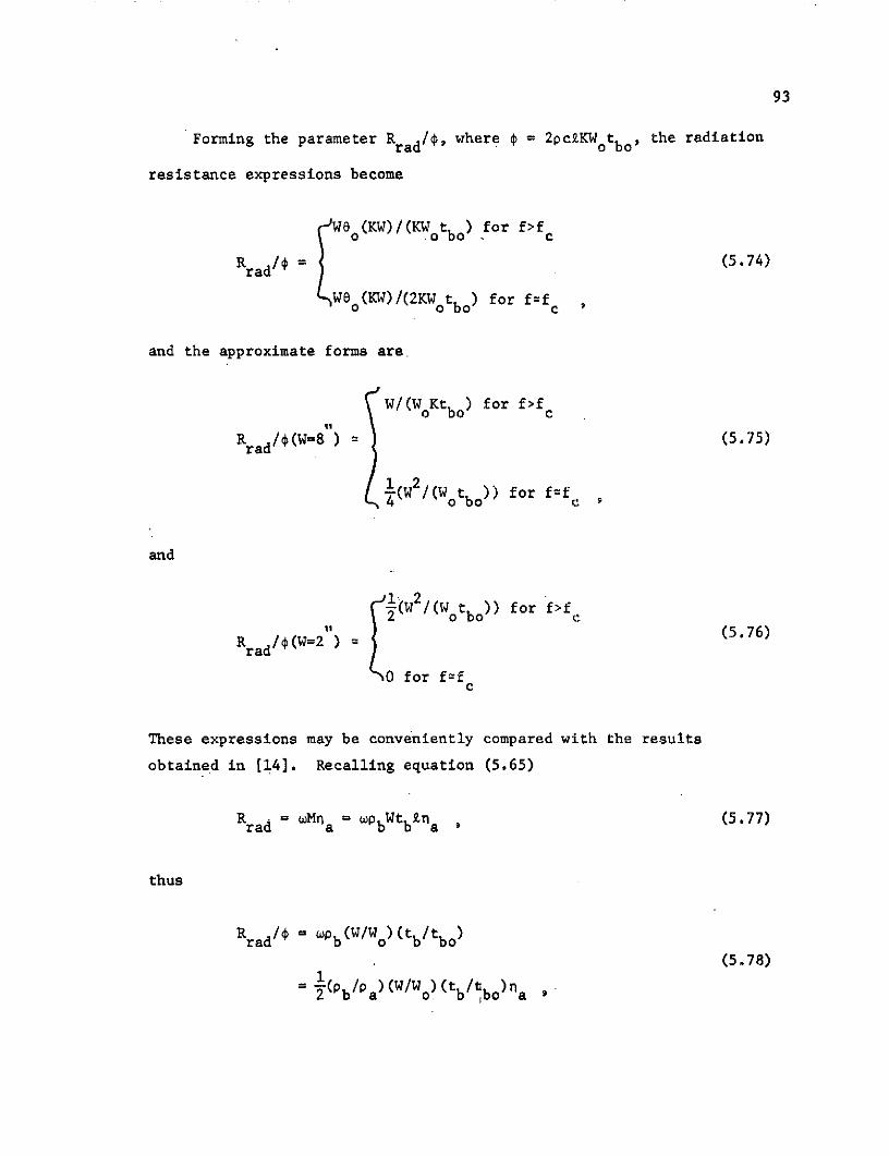
Forming the parameter Rrad/4, where = 2pcKWotbo, the radiation
resistance expressions become
We (KW)/(KW t ) for f>fo o bo c c
Rrad/0 = (5.74)
We o(KW)/(2KWotbo) for f-fe c
and the approximate forms are
W/(WoKtbo) for f>fe
R /ad(W=8 ) = (5.75)
rad2
1(W /(W t bo)) for f=f
and
(5.76)-i(w2/(Wotbo)) for f~fc
rad/ /(W= 2 (5.76)
0 for f=fc
These expressions may be conveniently compared with the results
obtained in [14]. Recalling equation (5.65)
Rrad = Mna = wPbWtbLna , (5.77)
thus
Rrad/0 - wPb(W/Wo)(tb/tbo)
(5.78)
= 2(Pb/a)(W/Wo)(tb/tbo)na a
94
where the value of na is found from Figure 5.20. Since Figure 5.20 is
based on pa/Pb = 1.55 x 10⁻³,which corresponds approximately to red oak,
the radiation parameter becomes
Rrad/ = 324na (W/Wo) (tb/tbo) (5.79)
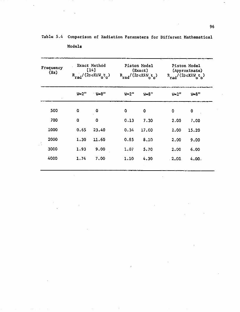
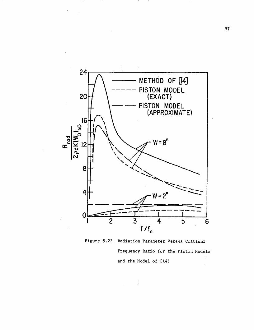
The values obtained for na from Figure 5.20 are given in Table 5.3 and
the values of the quantity Rrad/4 for W = to 1 inch are given in
Table 5.4, and plotted in Figure 5.22. From Figure 5.22 it is observed
that the theoretical trend of [14] which predicts that the major con-
tribution to the radiation parameter for the wider board is concentrated
in the vicinity of the critical frequency, while that for the narrower
board is spread out, is also apparent from the simple piston model.
The piston model is noted to exhibit the theoretical trends while
allowing quite simple computations of the radiated sound power.
5.5.1 A Comparison of the Radiation Characteristics of Wide and
Narrow Beams
The radiated sound power for two beams of four and eight inch
widths is of interest. The beams are excited across their width at a
blade passage frequency of 240 Hz, The beams are assumed to be of the
same material and the same length (five feet). The mean-square veloc-
ity - length product (<V2>£) is assumed to be constant and the velocity
magnitude and frequency spectra are assumed to be the same for each
beam. The beams are assumed to radiate from an infinite baffle.
95
Table 5.2 Radiation Efficiency Parameter for Different Values of KW
for Each Beam
f (KW) e (Kw) (KW) e (Kw)(Hz) (w-8") (W-8") (W2") (w=2")
500 1.80 0.40 0.46 0
700 2.62 0.60 0.66 0.02
1000 3.75 1.00 0.93 0.08
2000 7.50 0.95 1.88 0.40
3000 11.00 1.00 2.80 0.75
4000 14.00 1.00 3.70 1.00
Table 5.3 Acoustic Loss Factor for Different Frequencies.
f na na(Hz) (W=2") (W18")
1000 1.00x10 3 9.00x10- 3
2000 2.00x10- 3 4.50x10⁻³
3000 3.00x10⁻³ 3.50x10⁻³
4000 2.70x10⁻³ 2.70x10⁻³
96
Table 5.4 Comparison of Radiation Parameters for Different Mathematical
Models
Exact Meth6d Piston Model Piston ModelFrequency 14] (Exact) (Approximate)
(Hz) R /(2pcWt ) R /(2pcWt R /(2cKAWt
W=2" "=8" W-2" W8" W=2" W8"11
500 0 0 0 0 0 0
700 0 0 0.13 7.30 2.00 7.00
1000 0.65 23.40 0.34 17.00 2.00 15.20
2000 1.30 11.60 0.85 8.10 2.00 9.00
3000 1.93 9.00 1.07 5.70 2.00 6.00
4000 1.74 7.00 1.10 4.30 2.00 4.00.
97
24METHOD OF [14]
----- PISTON MODEL20 (EXACT)
- - PISTON MODEL(APPROXIMATE)
16 -- \o
T 12 W = 8"
0
0 . -- - -i I2 3 4 5 6
f/fc
Figure 5.22 Radiation Parameter Versus Critical
Frequency Ratio for the Piston Models
and the Model of [141
98
Equation (5.13) gave the radiated sound power for this case as
Pa = Rad <V2> = (R/rad)(<V >) . (5.80)rad rad
The values of the radiation resistance for the three frequency ranges
are given in.Table 5.1 for the baffled beam as
pcWBo(KW) for f>fe
rad = PcWkeo(KW) for f=f (5,81)
pcW2 (KW) for f<fe
for the square piston model based on beam width.
Defining the radiation efficiency as
a = R /(pc£W) , (5.82)rad .
the sound power may be written as
Pa = c(pcW) <£Z2> . (5.83)
Table 5.5 is obtained from Figure 5.15 for a blade passage fre-
quency of 240 Hz and harmonic frequencies for the two beams under
consideration. A plot of the radiation efficiency (a) versus frequency
for the eight and four inch wide beams is shown in Figure 5.23.
99
Table 5.5 Radiation Efficiency for Different KW Values of Each Beam
8 8f K KW KW o o
(W-8") (W=4") (W-8") (W-4") (W-8") (W-4")
240 0.11 0.88 0.44 0 0 0.02 0
480 0.22 1.76 0.88 0.30 0.09 0.08 0
720 0.33 2.64 1.32 0.67 0.15 0.34 0.08
960 0.44 3.52 1.76 0.92 0.35 0.92 0.35
1200 0.55 4.40 2.20 1.10 0.50 1.10 0.50
1440 0.66 5.30 2.64 1.12 0.65 1.12 0.65
1680 0.77 6.20 3.10 1.05 0.80 1.05 0.80
1920 0.88 7.00 3.50 1.00 0.92 1.00 0.92
2160 0.99 >7.00 3.96 1.00 1.05 1.00 1.05
2400 1.10 - 4.40 1.00 1.10 1.00 1.10
2640 1.21 - 4.85 1.00 1.12 1.00 1.12
2880 1.32 - 5.30 1.00 1.12 1.00 1.12
3120 1.43 - 5.65 1.00 1.10 1.00 1.10
3360 1.54 - 6.20 1.00 1.05 1.00 1.05
3600 1.65 - 6.60 1.00 1.00 1.00 1.00
3840 1.76 - 7.00 1.00 1.00 1.00 1.00
100
1.00
W= 8" W= 4"
b 0.10
/
0.01100 1000 10000
f(HZ)
Figure 5.23 Radiation Efficiency Versus Frequency for
the Eight and Four Inch Beam Widths
101
It has been observed experimentally that the force-frequency
characteristics of the input force (F) and the frequency response
characteristics of typical boards (H ) are such that the acceleration
-2response of the board (<a >) is essentially constant over a wide fre-
quency range. These quantities are in general related by
Sy () = Sf (W) IH()12 , (5.84)
where
S f() = input power spectral density = F(w)/T,
S (w) = output power spectral density = Y(w)/T.
The quantities F(a) and Y(w) are the Fourier transforms of the input
function F(t) and the response function y(t), respectively. In terms
of the radiation resistance, the power expression for a constant
acceleration - frequency spectrum is
Pa = R <2> Rrad <a >/ , (5.85)
since for single frequency components.
-2> -2 2<> <a >/ . (5.86)
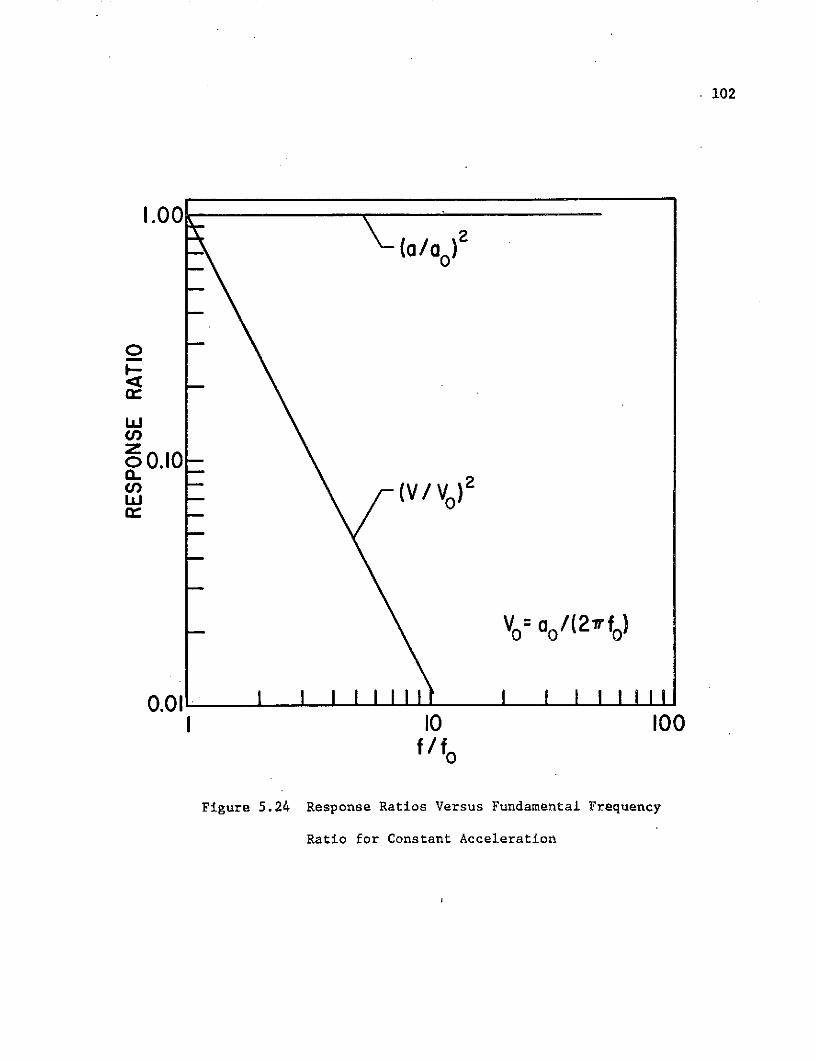
Thus, for constant acceleration response, the mean-square velocity
2decreases with frequency as Figure 5.24 shows the mean-squaredecreases with frequency as 1/w . Figure 5.24 shows the mean-square
102
1.00
-(a /a)2
0. I
0.01
10 100
f/fo
Figure 5.24 Response Ratios Versus Fundamental Frequency
Ratio for Constant Acceleration
103
velocity frequency response under this assumption, plotted against a
dimensionless frequency parameter f/fo . It is convenient to take fo
as the fundamental blade passage frequency. Noting that V = a /,o o
the velocity ratio can be written as
2 2 2(V/V ) = l/(W/ )2) = /(f/f)2, (5.87)
where V = a / = 2nf .
Recalling the expression for radiated power
Pa = R <2> = (R /9) <V2/V>- (<V2>Y)rad rad o o
and using equation (5.83), gives
Pa = pcWo <V2/V2> (<-2>,) (5.88)o o
The variables in equation (5.88) are the product o<V V2> and the beamO
-2width (W) since the quantity <V >k is assumed to be constant. Com-o
binirg the radiation resistance curves of.Figure 5.23 and using Figure
5.24 for the velocity variation, results in Figure 5.26, which is a
plot of o<V 2/V>(W/Wo) versus the frequency ratio f/fo . The frequency
variation in the velocity term of equation (5.88) is accounted for by
the factor (<V /V >) and the velocity amplitude, which depends on beam
-2length, is taken into account by the term <2 > shown in Figure 5.25.
0o
The frequencies that contribute to the overall power-output are
noted from Figure 5.26 to be; (a) the fourth harmonic (f/fo=4) for the0
104
1.0
0.8
0 .6I>
'/0.4
0.2-
0 2 3 4 5 6 7 8 9 101 (FEET)
Figure 5.25 Mean-square Velocity Ratio Versus Beam
Length for Constant <92 >2
105
1.00
S - 'W= 8"
/C ° /I/ \
S 0.10 \
- W= 4"
0.012 3 4 5 6 7 8 9 10
f/fo
Figure 5.26 Acoustic Power Parameter Versus Fundamental
Frequency Rati for the Eight and Four Inch
Beam Widths
106
eight inch beam, and (b) the fourth, fifth, and sixth harmonics
(f/fo = 4, 5, 6) for the four inch wide beam.
The discrete frequency sound power levels (L ) can be obtained by
defining a suitable reference power (Po) and performing the operation
10 loglO(Pa/Po), thus
Lw(f/f o ) = 10 log (Pa/P o)
= 10 logl 0 [(<V2 /V>W) (pc) (<V2 >)/Po
or
Lw(f/fo ) = 10 loglo0[<V2/V2>W] + 10 loglo0 <Ve>]
(5.89)
+ 10 loglO[pc/Po]
where the first term is obtained from Figure 5.26 and the second term
is specified experimentally or calculated from energy considerations.
When the value of <V2>, the mean-square velocity, is known as a
function of frequency for the board under consideration, equation (5.89)
- .. - . ... ....-- ------ - ---- -- I I - -. _ __ --- - - _---_-
= imsx znzn La-~----~-- ---- ------
, 6.--- --- .BOARD LENGTH5 -60 171 .... I II BOADL NTH - 5I I - -
dB dB 100 160 20 400 630 1.0 1.K 2.5( 4.0K 6.3K - K -K 1THIRD-OCTAVE-BAN CENTER FREQUENCY IN Hz
Figure 6.21 Comparison of Sound Pressure Levels for
Damping Treated and Untreated Boards
Ln
157
The bar graph of Figure 6.22 shows the effect of each damping
agent tested on the resulting anvil vibration (g) level. The neoprene
and constrained layer type damping were the most effective, reducing
the level approximately 15g from the untreated level. Theoretically,
damping treatments are effective methods for reducing board and machine
component vibration and the corresponding contribution to the total
noise. Friction, excessive sensitivity to temperature, and wear
problems make damping treatments difficult to apply in practice.
The effect of adding constraint mechanisms to physically restrain
the board from moving (vibrating) at the point of application has been
investigated. A constraint, such as a feed roller, may influence board
vibration by:
(1) Acting as a simple line constraint having no effect on the
magnitude of the vibration transmitted beyond it. The modes of board
vibration adjust so that a nodal point situates itself at the point of
constraint. A number of constraints placed along the feed beds
effectively raise the frequency of vibration and thus the frequency
of the sound produced.
(2) Acting as barrier to outward propagating vibration and
effectively decreasing the dynamic board length. To achieve this con-
dition a massive contact with the board is required, applied over a
large area.
(3) Acting as an energy absorber at the point of contact. The
chipbreaker mechanism exhibits this effect to some degree.
The conventional steel input and output feed roller mechanisms
used on planers act primarily as a simple line constraint described in
20
z 15
- 10
5-
UNTREATED RED NEOPRENE CONSTRAINEDRUBBER LAYER
TYPE OF TREATMENT
Figure 6.22 Effect of Damping Treatments on Anvil Vibration
00I
159
paragraph (1). Less conventional feed rollers constructed of rubber
could well exhibit the properties discussed in paragraphs (2) and (3)
and be valuable in dealing with planer noise.
For experimental purposes, a foam filled rubber tire and steel
plate arrangement was designed to perform the previously cited func-
tions to some degree, i.e., tend to (1) attenuate outward propagating
vibration by reflecting the vibratory waves, and (2) absorb energy by
virtue of the foam filled rubber tire and thus reduce the energy dis-
sipated as sound. With moderate force exerted, the tire deflects form-
ing a tire flatness, which is quite effective in attenuating the spread
of vibratory energy beyond the tire-plate. The tire itself also ab-
sorbs considerable vibratory energy. Sound pressure level and acceler-
ation measurements were made on the portion of the board extending
beyond a particular tire-plate suppressor. An acoustic enclosure was
utilized to reduce the sound eminating from the inner portion of the
board to levels well below the signal of interest. Figure 6.2, dis-
cussed previously, shows the experimental arrangement with the board
being excited by a mechanical vibrator with a square wave input. The
vibration insertion loss was detected by accelerometers located on
either side of the tire-plate system. An 18 dB insertion loss was
obtained with moderate loading of the tire and a similar 18 dB reduc-
tion in noise level was observed.
Such a tire-plate system can be easily installed on existing
roughing and cabinet type planers or incorporated into the feed works.
In conjunction with a moderate size acoustical enclosure, a tire-plate
suppression system has reduced noise levels in excess of 15 dBA in
160
industrial applications. Considerable work remains to be done in this
area, especially concerning the physical aspects of the tire in regard
to energy absorption.
6.6.3 Acoustic Enclosures
One means of obtaining substantial noise reduction for the planer
is the installation of a total or partial acoustic enclosure. For most
planing operations the acoustic energy radiated is concentrated between
500 and 5000 Hz. In this frequency range, a combination of absorbing
material and a housing of moderate stiffness and mass provides excellent
attenuation when the source is totally enclosed. The planer, however,
must have an area left open for input and output operations. Since
these "holes" greatly decrease the effectiveness of an enclosure, the
area of the opening must be minimized with respect to the total en-
closed area for maximum enclosure benefit. The adverse effect of the
opening also depends to a large degree on the frequency of the sound
energy being contained and absorbed within the enclosure. A guide to
the effectiveness of an enclosure that can be expected with respect to
opening sizes and acoustical absorbing surface area is given by (33]
and is repeated in Table 6.2.
An enclosure composed of several segments was used to evaluate the
maximum noise reduction obtainable for an enclosure having minimal
openings for feed purposes. The relative importance'of each section of
the enclosure was obtained by systematically removing and replacing
various sections. Photographs of the enclosure are shown in Figure 6.23.
Since the total length of the enclosure was equal to the length of the
machine, the board length became increasingly important. The amount of
161
Table 6.2 Noise Reduction for Acoustically Lined Plywood Enclosures
with Untreated Openings
Noise Reduction (dBA)Hole Area Fiberglass Treated Plywood Thickness
(% of Total Area) Area (%)1/2" 3/4" 1"
.1% 25% 13.0 18.0 20.0
50% 16.0 20.0 23.0
75% 18.0 23.0 25.0
100% 19.5 24.0 27.0
1% 25% 10.0 14.0 14.0
50% 13.0 17.0 17.0
75% 15.0 18.5 18.5
100% 17.0 20.0 20.0
5% 25% 7.0 9.0 9.0
50% 10.0 13.0 13,0
75% 11.5 14.0 14,0
100% 13.0 15.0 15.0
10% 25% 5.0 5.0 5.0
50% 8.0 8.0 8.0
75% 9.0 9.0 9.0
100% 10.0 10.0 10.0
162
I -Z
4i~:'~ sbi~~j ' F
ii LiFigue 623 couticEncosur fo SigleSurace
163
absorption obtainable was dependent upon the portion of the board that
was enclosed at any instant of time. Since vibrational energy spreads
through the board, the noise level at the operator position is dependent
upon the percentage of the board that is within the enclosure. Noise
levels for boards of length less than the machine length were signifi-
cantly reduced, while the reduction for locnger boards was considerably
less. Boards whose length exceeded the length of the enclosure pro-
duced sound levels which varied with the position of the board with
respect to the enclosure. The sound levels were noted to steadily de-
crease as the longer boards submerged into the enclosure until the
leading end of the board began to emerge from the output side of the
planer.
The effectiveness of the enclosure decreases with increasing board
length as shown in Figure 6.24. For boards of length greater than three
feet, the noise level varied with position as indicated in Figure 6.25,
In order to evaluate the relative importance of each section of
the enclosure, measurements were taken with different sections removed.
Figure 6.26 shows the reduction in noise level for two and six feet
long boards as the various sections of the enclosure are added. The
directivity characteristics, shown in Figure 6.27, remain essentially
the same for operation with and without the acoustic enclosure. Direc-
tivity characteristics, shown in Figure 6.28, for different board widths
would be expected to maintain a similar relationship for operation with
the acoustic enclosure.
BOARD WIDTH= 8"m
105--J
NO ENCLOSUREUJbi
Uj
10 0
m ENCLOSURE
2 3 4 5 6BOARD LENGTH (FEET)
Figure 6.24 Sound Pressure Level Versus Board Length for
Operation with and without an Acoustic Enclosure
, BOARD LENGTH =8'
"I00- BOARD WIDTH =8"-J
Lii-J
5 95n
z
8 90-a-
BOARD BOARD BOARDENTERING MIDWAY EXITING
0 0.25 0.50 0.75 1.00(ELAPSED TIME FROM BEGINNING OF CUT)/(TOTAL CUT TIME)
Figure 6.25 Sound Pressure Level Versus Board Position with
Respect to the Enclosure
0%
105 6EG 0m BOARD LENGTH=
BOARD WIDTH 8"
1j00-
Cn
S95
90-
FULL LOWER LOWER LOWER NOENCLOSURE (BACK) (FRONT) (FRONT ENCLOSURE
AIND BACK)ENCLOSURE SECTIONS REMOVED
Figure 6.26 Relative Importance of Different Sections
of the Acoustic Enclosure
BOARD LENGTH = 5'IB10 -BOARD WIDTH = 8"
105 -, NO ENCLOSURE-j
,W0 0
95-95
a9 ENC;LOSUR.0 90
n 85
I I I I2 3 4 5
MICROPHONE LOCATION
Figure 6.27 Directivity Characteristics for Operation with
and without the Acoustic Enclosure
110o BOARDWIDTH
LU 161
Sloo 8"cOU)
4"
90- 2"0o)
2 3 4 5MICROPHONE LOCATION
Figure 6.28 Directivity Characteristics for Different Board Widths
Co
169
7. COMPARISON OF THEORETICAL AND EXPERIMENTAL RESULTS
The important result obtained in the development of a model for
board vibration for the special case of a periodic forcing function was
given by equation (4.50) as
2 c sin(nux/z)sin(nrxo 1) 17Y(x,w) = 2 2
Pb n=l wn 2 (1-(w/nW)2 +2
S Ao(Jo )6(w-jw ) (7.1)
for the response in the frequency domain. The response at each fre-
quency (j o) is seen to be weighted by the frequency response function
of the beam. Thus the frequency spectrum of board vibration for the
planer is a discrete spectra with peaks occurring at each harmonic of
the blade passage frequency with the amplitude governed by the nearness
of these forced frequencies to natural resonant frequencies of the
board. Figure 3.6 indicates the close agreement of the vibration spec-
tra of the board with that predicted by equation (4.50). The excellent
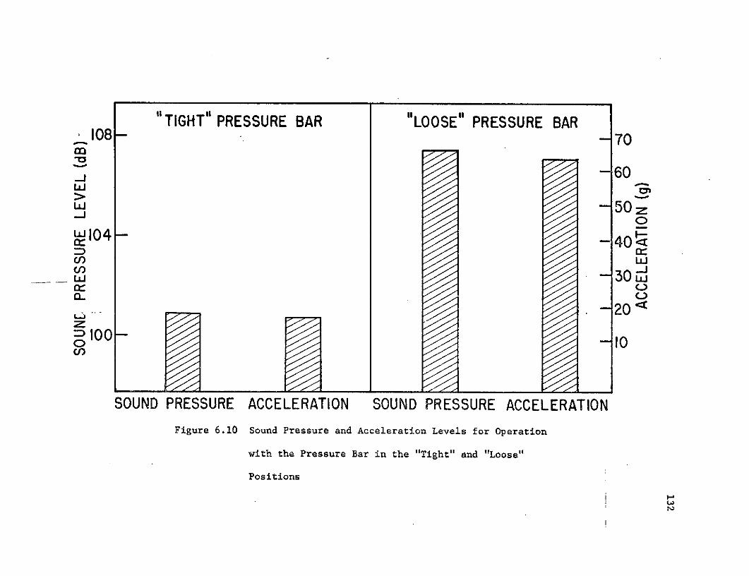
correlation of the sound and acceleration spectra shown in Figures 6.15
and 6.16, indicates the importance of board radiation as a noise gener-
ation mechanism as well as bearing out the theory for cutterheads having
four and six knives.
The important experimental result of a six decibel increase in
overall radiated sound power per doubling of board width was formulated
in terms of a source strength parameter. This source strength was
determined to be proportional to board width near the critical frequency
170
resulting in equation (6.3) for the sound power level proportionality,
i.e.;
LW n 10 log (Qs)2 , 20 log(W) (7.2)
Figure 3.7 illustrated this increase along with experimental values
of radiated sound power.
For frequencies near the critical frequency, where the sound
radiation is concentrated, the piston model of Chapter 5 gave the sound
power output as
L= 10 logl 0 (W2) + 20 logl 0 (fo)
-2+ 10 loglo(<Vo>) - 10 logl0(f)
+ 10 logl 0(r a/2Po) (7.3)
In the immediate vicinity of the critical frequency equation (7.3) can
be.written in terms of the proportionality;
L (f=f c) = 20 logl0(W) (7.4)
Thus, the theoretical acoustic power produced is also observed to
depend primarily on beam width and increases six decibels for each
doubling of width.
The experimental values obtained for the radiated sound power
level (overall), given in Figure 3.7, were obtained by measuring the
171
average sound pressure level over a hypothetical hemispherical surface
and accounting for the particular environment in accord with [11]. The
contributions to the radiated power occur at the blade passage frequency
and harmonics, with the major contributions being near the critical fre-
quency.
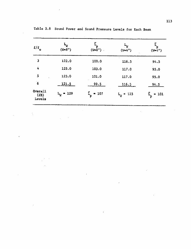
In Section 5.5.2 the actual radiated power for the four and eight
inch beam widths was computed. Contributions from the third, fourth,
fifth, and sixth harmonics were totaled to obtain the overall sound
power level. These levels were then adjusted according to [11] to give
the following values for the average sound pressure level at a five
foot radius;
L (W = 4) = 101 dB
L (W = 8) = 107 dB
which are in good agreement with the experimental results
L (W = 4) = 99 dB
L (W = 8) = 105 dBP
measured five feet from the machine centerline. The theoretical
accuracy could be improved by obtaining an exact measure.of the
-2quantity £<V0> which was assumed to be unity in this example.0
172
8. SURMARY AND CONCLUSIONS
Several sources of planer noise have been identified, the major
sources being board vibration, rotational noise, and anvil vibration.
For most planers the board -radiation dominates as evidenced by the six
decibel increase in noise level per doubling of board width and the
excellent correlation between the sound and board vibration spectra.
The board length did not directly affect the radiation since the energy
is distributed along the length of the board. The energy input to the
board by the cutterhead is independent of board length but increases
with increasing board width.
The vibration model developed in Chapter 4 is valid strictly for
slender beams. The transition from a beam to a plate is generally
defined to occur when W/Z > 1/10. The model is valid for board widths
up to about one foot, which is usually the case for roughing planers.
Panels (W/k > 1/10) can be analyzed by a similar modal approach, allow-
ing for vibration parallel as well as perpendicular to the cutterhead.
Special attention was given to the case of periodic forces since this
is typical of most cutterheads. The vibration model serves as a guide
to cutterhead design since the relationship of the forced harmonics to
the beam resonances governs sound radiation near the critical frequency.
Non-periodic forcing functions obtained by shear type cutterheads can
also be compared with standard heads on a vibration basis.
The radiation model developed in Chapter 5 combines the phase cell
concept of structural vibration in terms of the critical frequency with
the classical radiation theory for rectangular pistons. This rectangu-
lar model is simplified to a square piston in most cases. The radiated
power was given by equation (5.13) as P = Rrad <2> where the radia-
tion resistance is dependent on the "Ka" factor, the structural area,
and constants of the medium. The velocity term is a mean-square space-
time average which, in a reverberant vibrational field, is assumed to
have the same average properties for each piston element.
In order to represent the radiated power by equation (5.13), the
modes are assumed to be excited by a random noise in a narrow bandwidth.
Aw centered on frequency w, and the space-time average transverse
velocities of the modes within the band are assumed to be equal. The
equation governing the pure-tone response of any single mode can be
written as the product (Z V m), where Z is the sum of the mechanicalmm m
and radiation impedances. The mechanical impedance is the impedance
of the simple resonator that represents one natural mode of the struc-
ture in vacuo. In the derivation of equation (5.13) for the radiated
sound power, small forces arising from internal dissipation and from
sound radiation pressure that could tend to couple the response of
modes were neglected.
The baffled piston radiation properties were extended in an
approximate manner to apply to the case of an unbaffled piston by using
an analogy with a freely suspended disk. Expressions for the radiation
resistance were obtained in three frequency ranges for both baffled and
unbaffled beams. The velocity term to be used in equation (7.3) was
approximated using energy methods valid for reverberant fields rather
than the more complex expressions of Chapter 4.
The radiation model consolidates and extends existing theory by
using the radiation properties of a rectangular piston exclusively.
174
The important result that the major contribution to the radiated sound
power is concentrated near the critical frequency for wide boards and
spread out for narrower boards is apparent in the simple piston model.
The piston model exhibits the important theoretical trends of the
complex model of Section 5.4.3, while allowing quite simple computa-
tions of the radiated sound power.
The physical parameters such as board width, critical frequency,
and board length-velocity product are easily observed from the piston
model. The six decibel increase per doubling of width is explained in
relation to the power controlling critical frequency. There was good
agreement with experimental power measurements.
The experimental study defines the effect of various sources and
parameters on the noise emitted in a manner which can be directly
applied to future machine design. The major source of planer noise
was determined experimentally to be board radiation caused by the
periodic impact of the cutterhead knives. Board width was found to
affect the sound levels by an increase of six decibels per doubling of
board width, which indicates the dependence of source strength upon
width.
The length of the board did not directly affect the noise levels
but had a pronounced effect on vibration level. The vibration levels
decreased with increasing board length indicating a spreading out of
vibratory energy. Board length did, however, become quite important
when an acoustic enclosure was utilized since an enclosure is effective
only for that portion of the board that is contained within the enclo-
sure. Thus, longer boards produced greater noise levels at the
175
operator position. For this reason enclosures of the type discussed
offer only limited noise reduction, the amount depending on the size
of the enclosure and the length of the boards being planed.
The most promising means of noise reduction are; (1) cutterhead
redesign, (2) vibration suppression, and (3) acoustic enclosures. .Each
of-these areas have been studied in detail and significant improvements
realized.
In general there has been excellent agreement between the theoreti-
cal and experimental results. Many of the concepts developed have been
tested experimentally and successfully implemented on production line
machines. The progress that has been made toward understanding the
mechanism of noise generation in planing operations can be extended
readily to other woodworking machinery.
176
9. RECOMMENDATIONS
The entire vibration model and phase cell concept of board
radiation can be extended to plates, which are typical of panels in
the woodworking industry. This study was not pursued since the noise.
emission from most panels can be controlled by an enclosure in the
vicinity of the cutterhead (most panels are less than four feet long).
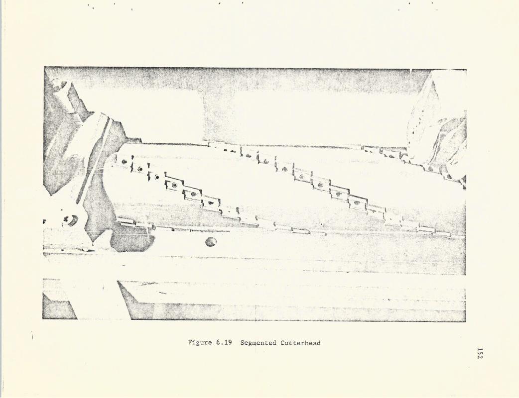
Additional study is needed in the area of cutterhead redesign,
since the exact effect of knife sharpness, helix angle, segmented knife
overlap, cutterhead speed, and cutterhead geometry on operational noise
levels is not known, although the results indicate that the ideal case
is that of a true, tightly wound, helix.
The vibration suppression techniques have not been analyzed in
detail in regard to the factors affecting the reflection, transmission,
and absorption of vibratory energy. The tire system could possibly be
designed to act as a dynamic vibration absorber which would absorb
energy over a wide frequency range, and thus substantially reduce the
noise output from the board. Modern day, high energy absorbing,
polymers could-possibly be used in an energy absorbing capacity, or
incorporated into tire construction.
Long range study areas include such revolutionary changes as the
use of laser beams to do many of the noisy and unsafe operations in
the woodworking industry with a significant reduction in waste and
waste products.
177
10. LIST OF REFERENCES
1. Barnoski, R. L. 1965. Response of Elastic Structures toDeterministic and Random Excitation. Technical ReportAFFDL-TR-64-199. Air Force Flight Dynamics Laboratory,Research and Technology Division Air Force Systems Command,Wright-Patterson Air Force Base, Ohio.
2. Beranek, L. L. 1971. Noise and Vibration Control. McGraw-HillBook Company, Inc., New York, New York.
3. Beranek, L. L. 1960. Noise Reduction. McGraw-Hill Book Company,Inc., New York, New York.
4. Bramer, T. P. C. 1969. Literature Survey: Noise Generation inWood Planing and Moulding Machines. Contract No. KJ/4M/107/CB78A, Technical Report No. C/C. 311 for The Ministry of Tech-nology, Sound Research Laboratories, Eastgates Colchester,Essex.
5. Chizherskiu, M. P., and S. I. G. Shkalenko. 1968. Experiments onNoise Reduction in Planers. Derev. Prom., No. 1, pp. 26-27.
6. Churchill, R. V. 1958. Operational Mathematics. McGraw-HillBook Company, Inc., New York, New York.
7. Cox, J. R. 1955. Quieting Wood Planers. Liberty Mutual Insur-ance Co., Research Center, Boston, Massachusetts.
8. Crandall, S. H., and W. D. Mark. 1963. Random Vibration. Aca-demic Press, New York, New York.
9. Cremer, L. 1953. Calculation of Sound Propagation in Structures.Acustica, Vol. 3, No. 5, pp. 317-335.
10. Greenwood, J. H. F. 1968. Noise Reducing Enclosures for a Planerand a Moulder. Woodworking Industry, Vol. 25, No. 11,pp. 19-20.
11. Hart, F. D., and J. S. Stewart. 1971. Noise Level Prediction forSimple and Complex Sources in the Industrial Environment.Presented and published in the proceedings of the IEEE AnnualMeeting, Cleveland, Ohio, pp. 731-737.
12. Hollowood, H. B. 1971. Electric Equipment Noise. Presented atthe Thirty-third Annual Meeting of the American Power Con-ference, Chicago, Illinois.
13. Hurty, W. C., and M. F. Rubinstein. 1964. Dynamics of Structures.Prentice-Hall, Inc., Englewood Cliffs, New Jersey.
178
14. Johnston, R. A., and A. D. S. Barrt. 1968. Acoustic and Internal
Damping in Uniform Beams. Journal of Mechanical EngineeringScience, Vol. 11, No. 2, pp. 117-127.
15. Kinsler, L. E., and A. R. Frey. 1962. Fundamentals of Acoustics.John Wiley and Sons, Inc., New York, New York.
16. Koch, Peter. 1964. Wood Machining Processes. The Ronald Press-Company, New York, New York.
17. Kozyakov, A. F. 1966. Noise Control in Woodworking Machines.Izvestiya Vysshikh Uchebniykh Zavedeniy, Lesnoy Zhurnal,No. 12, pp. 124-129.
18. Kuleskov, L., and V. Grirkov. 1966. Influence of Knife Form onthe Level of Noise while Planing. Woodworking Industry,Vol. 2, No. 5, pp. 11-12.
19. Liegman, E. 1956. Noise Research on a Planer. Holz als Roh-undWerkstoff, Vol. 14, No. 4, pp. 121-135.
20. Lyon, Richard H. 1962. Sound Radiation from a Beam Attached toa Plate. J. Acoust. Soc. of America, Vol. 34, No. 9,pp. 1265-1268.
21. Lyon, Richard H., and Gideon Maidanik. 1962. Power Flow betweenLinearly Coupled Oscillators. J. Acoust. Soc..of America,Vol. 34j No. 9, pp. 623-639.
22. Maidanik, Gideon. 1962. Response of Ribbed Panels to ReverberantAcoustic Fields. J. Acoust. Soc. of America, Vol. 34, No. 6,pp. 809-826.
23. Mazur, V. F., and 0. K. Kurtun. 1966. Noise Production in RotaryCutters. Derev. Prom., No. 12, pp. 34-39.
24. Morse, P. M., and K. U. Ingard. 1968. Theoretical Acoustics.McGraw-Hill Book Company, Inc., New York, New York.
25. Pahlitzsch, G. 1956. Research on Noise Formation in Wood PlaningMachines. Holz als Roh-und Werkstoff, Vol. .14, No. 4,pp. 90-95.
26. Richards, E. J., and D. J. Mead. 1968. Noise and Acoustic Fatiguein Aeronautics. John Wiley and Sons, Inc., New York, NewYork.
27. Schmutzler, W. 1967. Noise Abatement in Woodworking. Holz alsRoh-und Werkstoff, Vol. 25, No. 4, pp. 130-131.
179
28. Smith, J. Howard. 1971. Noise in the Woodworking Industry - AReview of the Literature. Forest Products Journal, Vol. 21,No. 9, pp. 82-83.
29. Smith, P. W., Jr. 1962. Response and Radiation of StructuralModes Excited by Sound. J. Acoust. Soc. of America, Vol. 34,No. 5, pp. 640-647.
30. Smith- P. W., Jr., and Richard H. Lyon. 1965. Sound and Struc-tural Vibration. NASA Contractor Report CR-160, NationalAeronautics and Space Administration, Washington, D. C.
31. Smith, P. W., Jr. 1964. Coupling of Sound and Panel VibrationBelow the Critical Frequency. J. Acoust. Soc. of America,Vol. 36, No. 8, pp. 1516-1520.
32. Sneddon, I. N. 1951. Fourier Transforms. McGraw-Hill BookCompany, Inc., New York, New York.
33. Stewart, J. S. 1972. Noise, Enclosures and the WoodworkingIndustry. National Hardwood Magazine, Vol. 46, No. 4,pp. 40-51.
34. Stewart, J. S., and F. D. Hart. 1972. Analysis and Control ofWood Planer Noise. Sound and Vibration, Vol. 6, No. 3,pp. 24-27.
35. Volterra, E., and E. C. Zachmanoglou. 1965. Dynamics of Vibra-tionse Charles E. Merrill Books, Inc., Columbus, Ohio.
36. Thomson, W. T. 1965. Vibration Theory and Applications.Prentice-Hall, Inc., Englewood Cliffs, New Jersey.
37. Thunnell, B. 1957. On Noise Problems with Woodworking Machinery.Stockholm, Sweden.
18.0
11. LIST OF SYMBOLS
A Radiating surface area of vibrating structure
Acc. Acceleration
A Fourier coefficient in series expansion of waveform0
A Area of reflecting room surfacesr
a Characteristic dimension of radiator
a Reference accelerationo
<a> Space-time averaged acceleration
BPF Blade passage frequency
b. Dimension of radiator
SOne-half the vector distance between monopole sources located
on each piston face
C Speed of sound in air
CB Transverse bending wave.velocity
C Generalized damping coefficient for the nth mode of beamn
vibration
c(x) Viscous damping coefficient.
d Length of rectangular piston element
dB Decibel
E Modulus of elasticity
ET Total stored vibrational energy
F(x,t) Beam excitation function
F(x,w) Fourier transform of F(x,t)
F { } Denotes Fourier transform operatione-
F { } Denotes inverse Fourier transform operatione
181
FR Beam radiation loading function
f Frequency in-Hertz
fc Critical beam frequency
fh Harmonic.frequencies present in.excitation signal
fn(x) Mode shape of beam vibrating in the nth mode
g Unit of measure for acceleration
gc. Acceleration due to gravity
H n() System frequency response function
H Hertz (cycles per second)
h System response to a unit-impulse
I- Area moment of inertia of beam cross section
i. v:T
J Zero order Bessel function
J1 First order Bessel function
j Integer
K Acoustic wave number =.w/CaKa Dimensionless product governing radiation
Kb Dimensionless product governing radiation
Kd Structural wave number = w/CB
K Generalized stiffness coefficient for nth mode of beam.
vibration
Ln(x,t) Generalized force corresponding to the nth mode of beam
vibration
Ln(x,w) Fourier transform of L (x,t) with respect to time
L Sound pressure level, referenced to 0.0002 pbar
Lp Space average of sound pressure levels
182
LW Sound power level, referenced to 10- 13 watts
a Beam length
M Total mass of beam
Mn Generalized mass corresponding to the.nth mode of beam
vibration
my. Millivolts
N Number of knives on cutterhead
N Number of contributing piston elements
n Integer
Pa Acoustic power radiated to the far field
P Reference.acoustic power, taken as 10-13 watts
n(w) Fourier transform of qn(t)
Qs Acoustic source strength
qn(t) Generalized coordinate corresponding to the nth normal
vibrational mode
R Room constant
Re{ I Denotes real part of quantity to be taken
RPM Revolutions per minute
R Radiation resistancerad
r Radius of radiating disk
S Surface area of baffled beam = W£
Sf System input power spectral density
SH Surface area of test hemisphere
S System output power spectral density
T Period of signal
t Real time
183
tb Beam thickness
tbo Reference beam thickness
t Instant of time0
V- Transverse.beam velocity
V Reference beam.velocity
<V2> Mean-square transverse beam velocity
W Width of beam orpiston element
Wo Reference width of beam or piston element
x Coordinate along beam length
xo Specific position along x,coordinate
Y(x,w) Fourier transform of.y(x,t) with respect to time
y. Coordinate perpendicular to beam length
y(x,t) Transverse displacement of beam
Z Radiation impedance
aAcoustic absorption coefficient
8 Coefficient typical of particular type of boundary conditions
6 Dirac delta function
6 Internal damping coefficient
SDamping factor
En Damping factor for the nth vibrational mode
na. Acoustic loss factor
nd Dissipation loss factor
8 Radiation efficiency function for square piston
83 Radiation efficiency function for rectangular piston
184
Aa Acoustic wavelength
x ns Modal.structural wavelength
x Structural wavelength
p Mass density
Pa Mass density of air
Pb Mass density of beam.
pc Specific acoustic impedance
a Radiation efficiency
T Time variable used in conjunction with convolution integral
0 Cross sectional area of beam
W Angular frequency
Sn. Natural vibrational frequency
At Small frequency increment centered on frequency w
C() Denotes differentiation with respect to time
(') Denotes second derivative with respect to time
( ) Denotes differentiation with respect to xIt
( ) Denotes second derivative with respect to x
Denotes convolution operation
Indicates the radiation resistance should be multiplied by a
factor of one for the baffled radiator and a factor of two