A TOPOLOGICAL SYSTEM FOR CODIFICATION OF RIVER BASINS IN TURKEY A THESIS SUBMITTED TO THE GRADUATE SCHOOL OF NATURAL AND APPLIED SCIENCES OF MIDDLE EAST TECHNICAL UNIVERSITY BY İBRAHİM ULUCAN IN PARTIAL FULFILLMENT OF THE REQUIREMENTS FOR THE DEGREE OF MASTER OF SCIENCE IN GEODETIC AND GEOGRAPHIC INFORMATION TECHNOLOGIES JUNE 2021
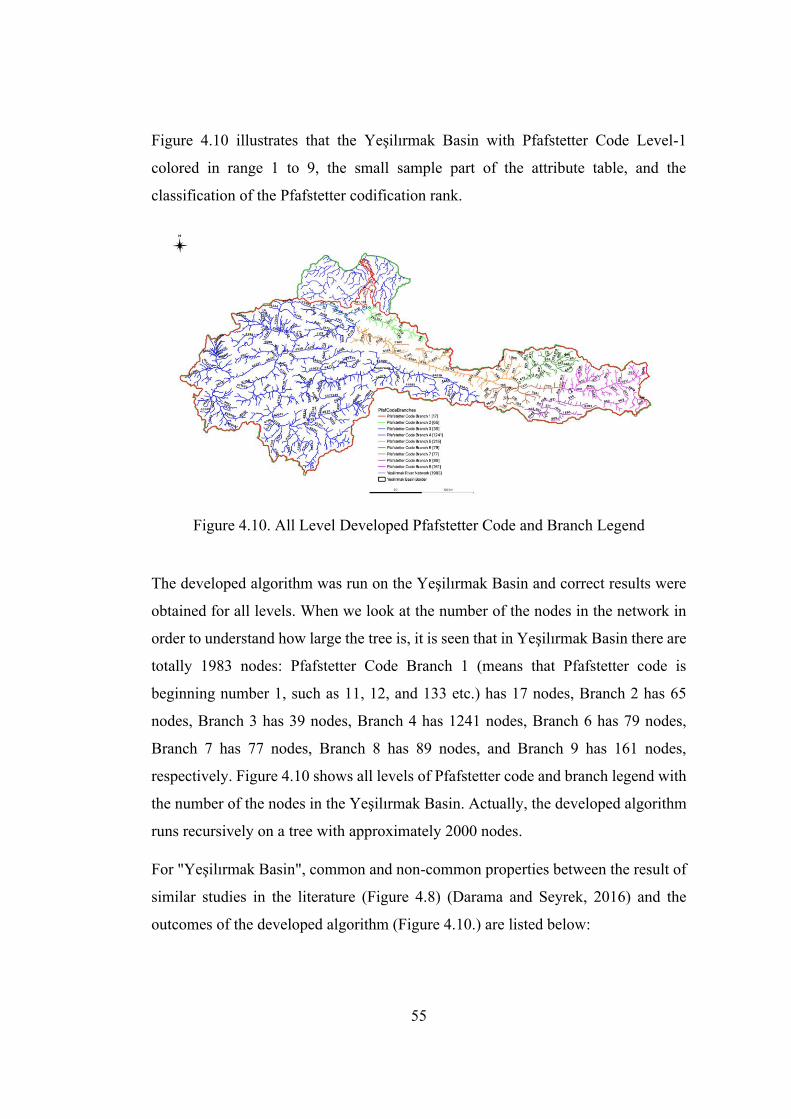
Transcript
A TOPOLOGICAL SYSTEM FOR CODIFICATION OF RIVER BASINS IN TURKEY
A THESIS SUBMITTED TO THE GRADUATE SCHOOL OF NATURAL AND APPLIED SCIENCES
OF MIDDLE EAST TECHNICAL UNIVERSITY
BY
İBRAHİM ULUCAN
IN PARTIAL FULFILLMENT OF THE REQUIREMENTS FOR
THE DEGREE OF MASTER OF SCIENCE IN
GEODETIC AND GEOGRAPHIC INFORMATION TECHNOLOGIES
JUNE 2021
Approval of the thesis:
A TOPOLOGICAL SYSTEM FOR CODIFICATION OF RIVER BASINS
IN TURKEY
submitted by İBRAHİM ULUCAN in partial fulfillment of the requirements for the degree of Master of Science in Geodetic and Geographic Information
Technologies, Middle East Technical University by, Prof. Dr. Halil Kalıpçılar Dean, Graduate School of Natural and Applied Sciences
Prof. Dr. Zuhal Akyürek Head of the Department, Geodetic and Geographic
Information Technologies
Prof. Dr. Zuhal Akyürek Supervisor, Civil Engineering, METU
Examining Committee Members: Prof. Dr. İsmail Yücel Department of Civil Engineering, METU
Prof. Dr. Zuhal Akyürek Department of Civil Engineering, METU
Prof. Dr. Pınar Karagöz Department of Computer Engineering, METU
Assoc. Prof. Dr. Yakup Darama Department of Civil Engineering, Atılım University
Assist. Prof. Dr. Semih Kuter Department of Forest Engineering, Çankırı Karatekin University
Date: 23.06.2021
iv
I hereby declare that all information in this document has been obtained and
presented in accordance with academic rules and ethical conduct. I also declare
that, as required by these rules and conduct, I have fully cited and referenced
all material and results that are not original to this work.
Name, Last name : İbrahim, Ulucan
Signature:
v
ABSTRACT
A TOPOLOGICAL SYSTEM FOR CODIFICATION OF RIVER BASINS
IN TURKEY
Ulucan, İbrahim Master of Science, Geodetic and Geographic Information Technologies
Supervisor : Prof. Dr. Zuhal Akyürek
June 2021, 79 pages
Recently, owing to incredible development in Geographic Information Systems
(GIS) and software fields, besides effectively using the network and topology
instruments, great advances have been made in the field of hydrologic coding
through robust interaction among multidisciplinary sciences. If all hydrological
properties can be combined in a network that has its own sui generis situation and
topological properties, meaningful and holistic analyses can be formed more easily.
Additionally, GIS topology is an essential phenomenon for performing different
types of network analysis, therefore the topological network model manages spatial
relationships by illustrating shapes as the graph of topological instruments (node,
edge, etc.) via computer geometry.
In this study, the Pfafstetter method, which stands out with its topological feature
and the most common hydrological codification systems all over the world, was
coded. It was written in Object-Oriented Program (OOP) language and formatted as
a binary tree data structure. The proposed code was applied to three different river
basins namely Çakıt Basin and Yeşilırmak Basin which are located in Turkey, and
vi
Thames River Basin which is located in the UK. It is observed that successful results
were obtained.
Keywords: Geographic Information Systems (GIS), Algorithm, Topology, River
Network, Pfafstetter Coding System
vii
ÖZ
TÜRKİYE'DEKİ NEHİR HAVZALARININ KODLANMASI İÇİN
TOPOLOJİK BİR SİSTEM
Ulucan, İbrahim Yüksek Lisans, Jeodezi ve Coğrafi Bilgi Teknolojileri
Tez Yöneticisi : Prof. Dr. Zuhal Akyürek
Haziran 2021, 79 sayfa
Son yıllarda, Coğrafi Bilgi Sistemleri (CBS) ve yazılım alanlarındaki büyük
gelişmeler ile özellikle ağ ve topoloji enstrümanlarının etkin bir şekilde
kullanılmasıyla, çok disiplinli bilimler arasındaki güçlü etkileşim ve iletişim
sayesinde, hidrolojik kodlama alanında büyük ilerlemeler kaydedilmiştir. Tüm
hidrolojik özellikler kendine özgü durumla topolojik özelliklere haiz bir ağ yapısında
birleştirilebildiği taktirde anlamlı ve bütüncül analizlere daha rahat kapı aralanabilir.
Ağ topolojisinin gücünün CBS ile birleşmesi ile çok zengin ve çeşitli imkanlara
olanak sağlanmış, bu bağlamda bilgisayar geometrisi ve grafik veri yapıları
aracılığıyla topolojik araçların (düğüm, kenar vb.) uzamsal ilişkileri etkin bir şekilde
yönetilebilir hale gelmiştir.
Bu çalışmada, topolojik özelliği ile ön plana çıkan ve dünya genelinde yaygın
kullanıma sahip hidrolojik kodlama sistemlerinden biri olan Pfafstetter yöntemi
kodlanmıştır. Bu bağlamda, Nesne Yönelimli Programlama (NYP) dili ile ikili ağaç
yapısına dayalı bir algoritma ile geliştirilmiştir. Geliştirilen algoritma, Türkiye'de
bulunan Çakıt Havzası, Yeşilırmak Havzası ve İngiltere'de yer alan Thames Nehri
Havzası üzerinde uygulanmıştır. Başarılı sonuçların elde edildiği görülmüştür.
viii
Anahtar Kelimeler: Coğrafi Bilgi Sistemleri (CBS), Algoritma, Topoloji, Nehir
Ağları, Pfafstetter Kodlama Sistemi
ix
To my lovely family
x
ACKNOWLEDGMENTS
I wish to express my deepest gratitude to my supervisor Prof. Dr. Zuhal Akyürek,
for not only her guidance, advice, criticism, encouragements, and insight throughout
the research; but also supporting me spiritually my challenges on all steps in terms
of GIS software and applications.
I would especially like to state that I used very useful information (Mapping, GIS,
DBMS, Topology, DEM, Flow Direction & Accumulation, TIN, Network, Shortest
Distance and D8 Algorithms etc.) that I learned in the Introduction to GIS (CE-413)
course I took from Prof. Dr. Zuhal Akyürek in all stages of this thesis. I also thank
Mr. Kenan Bolat for the useful applications in the laboratory within the scope of this
course. If I had not taken the Introduction of GIS, this thesis would not be possible
successfully. Also, I would like to special thank Mr. Çağrı Hasan Karaman for
providing useful data (DEM, River Network, etc.) from HIDRO-ODTU.
I am completely appreciative of my family. I would like to thank especially my dear
wife and two lovely little kids for their endless love and their consideration for my
achievements.
This work has the feature of providing the topological capability to the HIDRO-
ODTU (Determination of Hydrological Cycle Parameters with a Conceptual
Hydrological Model, TUBITAK 115Y041).
xi
TABLE OF CONTENTS
ABSTRACT ............................................................................................................... v
ÖZ ........................................................................................................................... vii
ACKNOWLEDGMENTS ......................................................................................... x
TABLE OF CONTENTS ......................................................................................... xi
LIST OF TABLES ................................................................................................. xiii
LIST OF FIGURES ............................................................................................... xiv
LIST OF ABBREVIATIONS ............................................................................... xvii
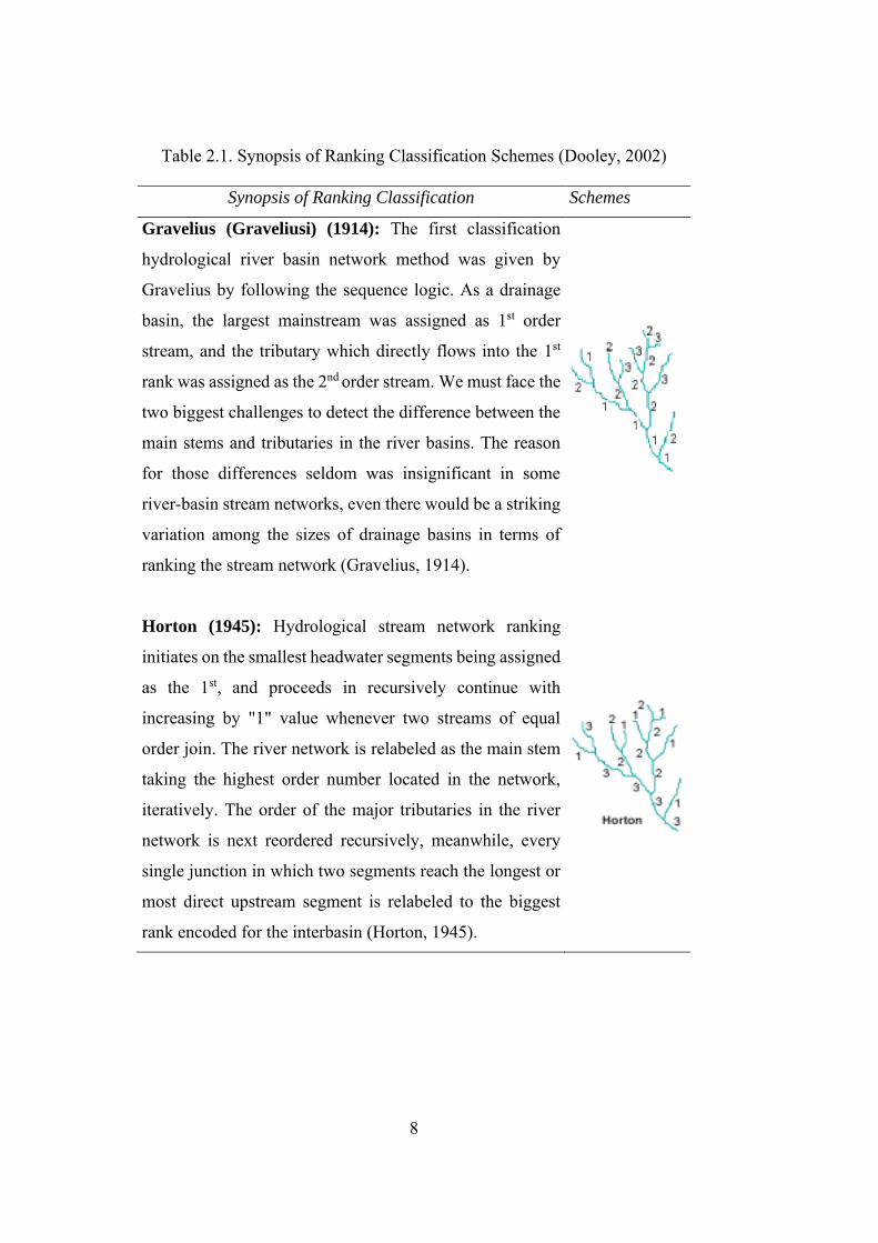
initiates on the smallest headwater segments being assigned
as the 1st, and proceeds in recursively continue with
increasing by "1" value whenever two streams of equal
order join. The river network is relabeled as the main stem
taking the highest order number located in the network,
iteratively. The order of the major tributaries in the river
network is next reordered recursively, meanwhile, every
single junction in which two segments reach the longest or
most direct upstream segment is relabeled to the biggest
rank encoded for the interbasin (Horton, 1945).
9
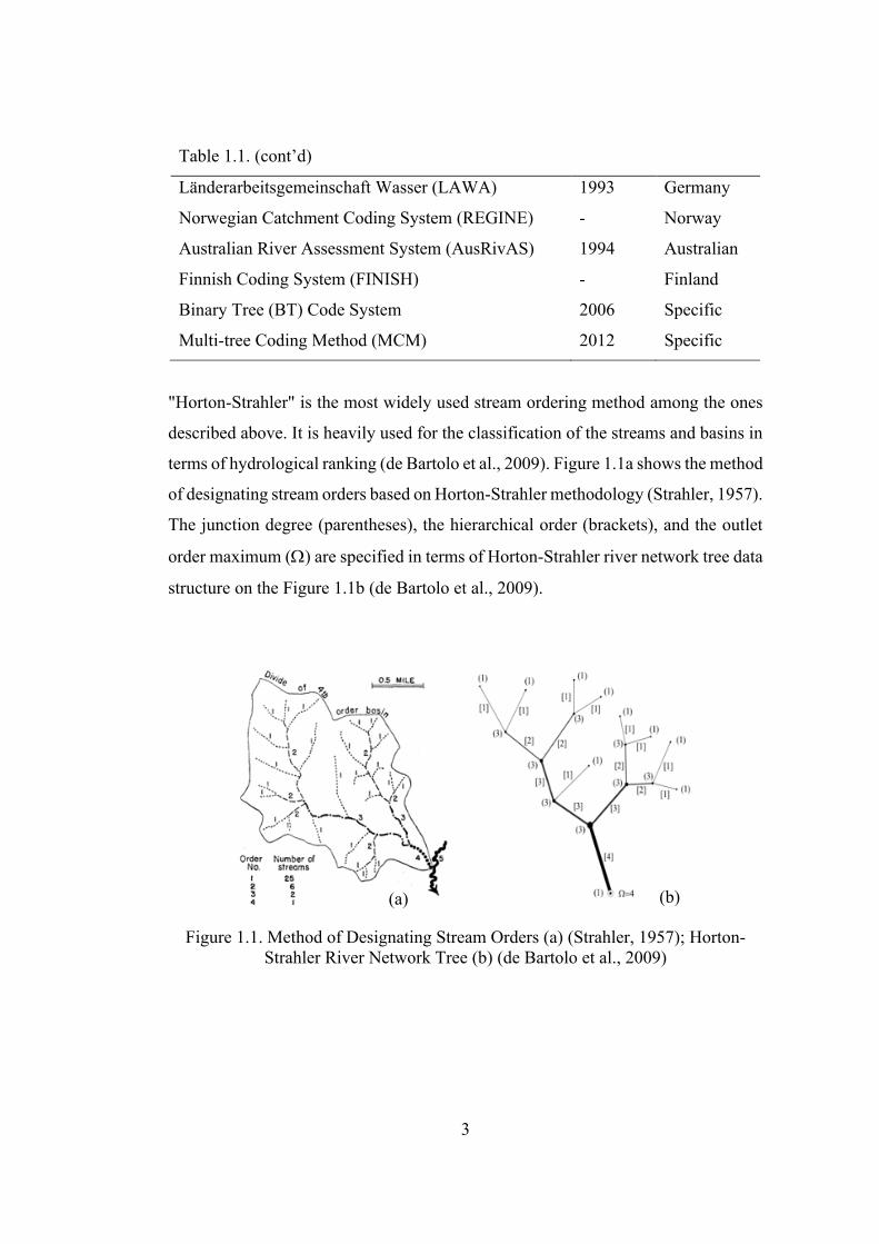
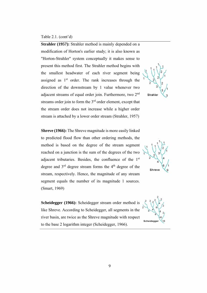
Table 2.1. (cont’d)
Strahler (1957): Strahler method is mainly depended on a
modification of Horton's earlier study; it is also known as
"Horton-Strahler" system conceptually it makes sense to
present this method first. The Strahler method begins with
the smallest headwater of each river segment being
assigned as 1st order. The rank increases through the
direction of the downstream by 1 value whenever two
adjacent streams of equal order join. Furthermore, two 2nd
streams order join to form the 3rd order element, except that
the stream order does not increase while a higher order
stream is attached by a lower order stream (Strahler, 1957)
Shreve (1966): The Shreve magnitude is more easily linked
to predicted flood flow than other ordering methods, the
method is based on the degree of the stream segment
reached on a junction is the sum of the degrees of the two
adjacent tributaries. Besides, the confluence of the 1st
degree and 3rd degree stream forms the 4th degree of the
stream, respectively. Hence, the magnitude of any stream
segment equals the number of its magnitude 1 sources.
(Smart, 1969)
Scheidegger (1966): Scheidegger stream order method is
like Shreve. According to Scheidegger, all segments in the
river basin, are twice as the Shreve magnitude with respect
to the base 2 logarithm integer (Scheidegger, 1966).
10
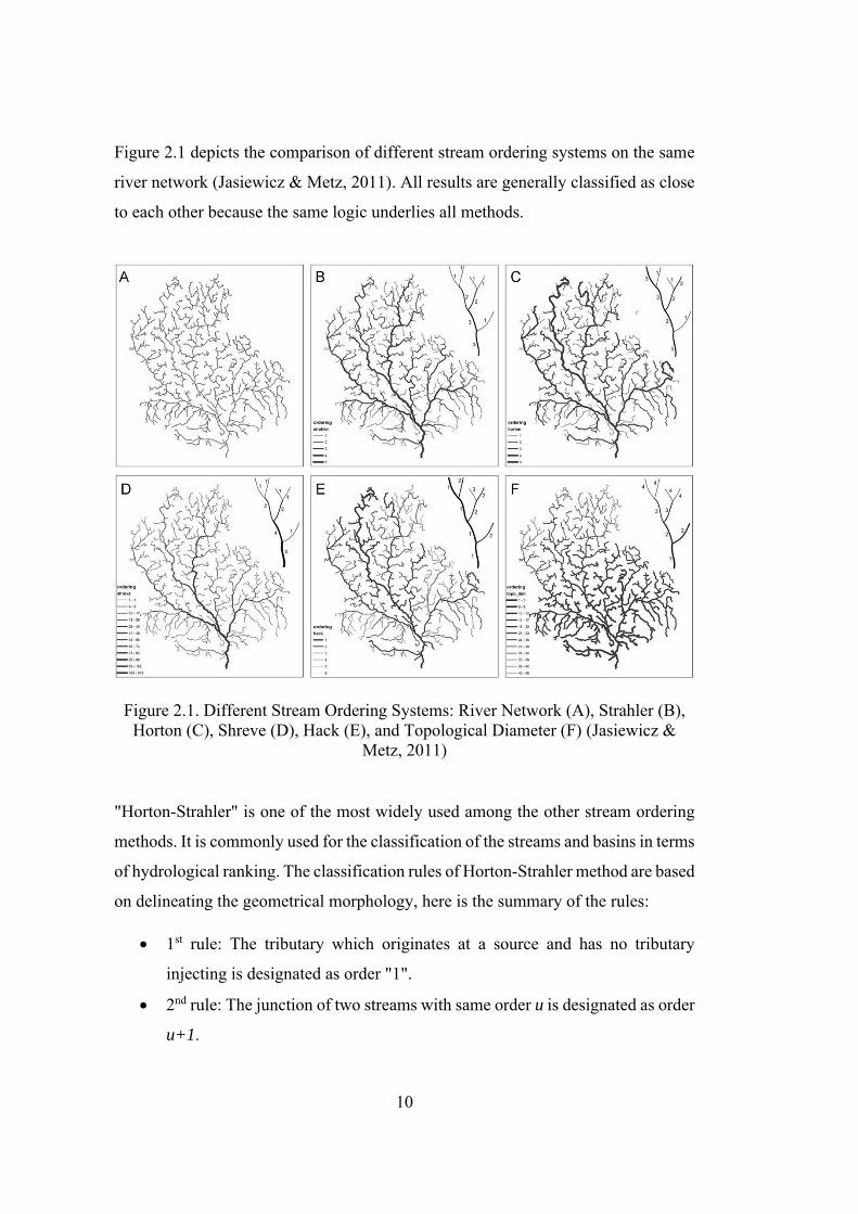
Figure 2.1 depicts the comparison of different stream ordering systems on the same
river network (Jasiewicz & Metz, 2011). All results are generally classified as close
to each other because the same logic underlies all methods.
Figure 2.1. Different Stream Ordering Systems: River Network (A), Strahler (B), Horton (C), Shreve (D), Hack (E), and Topological Diameter (F) (Jasiewicz &
Metz, 2011)
"Horton-Strahler" is one of the most widely used among the other stream ordering
methods. It is commonly used for the classification of the streams and basins in terms
of hydrological ranking. The classification rules of Horton-Strahler method are based
on delineating the geometrical morphology, here is the summary of the rules:
• 1st rule: The tributary which originates at a source and has no tributary
injecting is designated as order "1".
• 2nd rule: The junction of two streams with same order u is designated as order
u+1.
11
• 3rd rule: The junction of two streams with unequal order u and v, where u<v,
is designated as order max (u, v).
The function of the classification rules formulated as:
1, u = v ; n = max (u, v) + u,v , where u,v = 0, u v
where n is the order of the network formed by two streams with unequal order both
u and v (Zhang et al., 2007).
In theory, encoding river network that is based on any of the above ranking methods
is such a basic programming issue, however; in practice, it is hard to find that real
river dataset has a verified connectivity between every single of the elements.
Generally, river ordering classifications are not commonly executed to watershed
networks or models, however; in cases where a topological encoding scheme has
been used to link the stream network into the watershed model, the transfer of such
attributes can be easily facilitated without the need to resort to any GIS software
(Dooley, 2002).
2.1.2 Topological Codification Systems
Within the scope of the network, basic topological relationships (connectivity,
adjacency, and enclosure) are of great importance in the context of our analysis by
establishing a relationship between the data set like the river network. Due to
advances in the processing and analysis of hydrological data with the help of the
developing GIS software, important attempts have been made throughout the world
in hydrological coding methods today. Some of these topological coding systems
will be mentioned here.
12
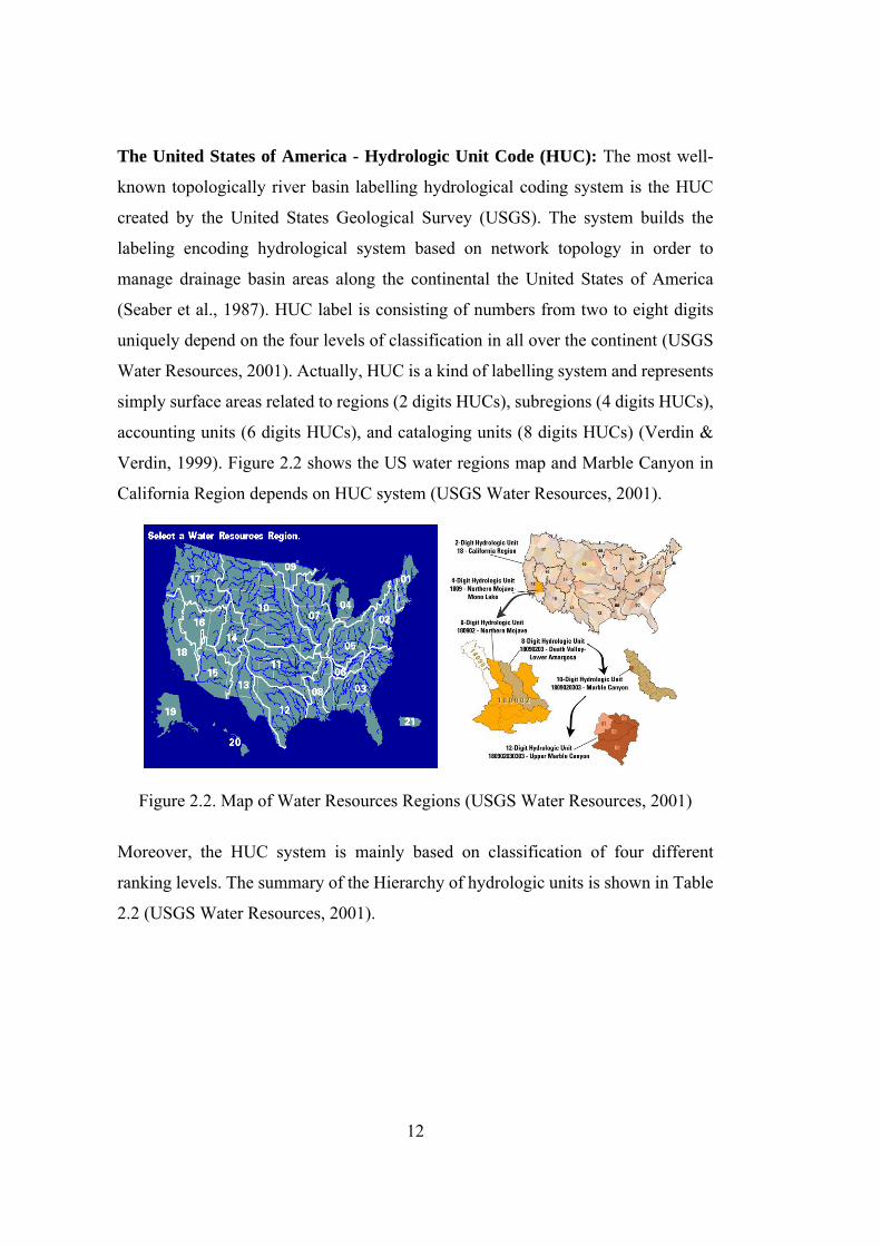
The United States of America - Hydrologic Unit Code (HUC): The most well-
known topologically river basin labelling hydrological coding system is the HUC
created by the United States Geological Survey (USGS). The system builds the
labeling encoding hydrological system based on network topology in order to
manage drainage basin areas along the continental the United States of America
(Seaber et al., 1987). HUC label is consisting of numbers from two to eight digits
uniquely depend on the four levels of classification in all over the continent (USGS
Water Resources, 2001). Actually, HUC is a kind of labelling system and represents
simply surface areas related to regions (2 digits HUCs), subregions (4 digits HUCs),
accounting units (6 digits HUCs), and cataloging units (8 digits HUCs) (Verdin &
Verdin, 1999). Figure 2.2 shows the US water regions map and Marble Canyon in
California Region depends on HUC system (USGS Water Resources, 2001).
Figure 2.2. Map of Water Resources Regions (USGS Water Resources, 2001)
Moreover, the HUC system is mainly based on classification of four different
ranking levels. The summary of the Hierarchy of hydrologic units is shown in Table
2.2 (USGS Water Resources, 2001).
13
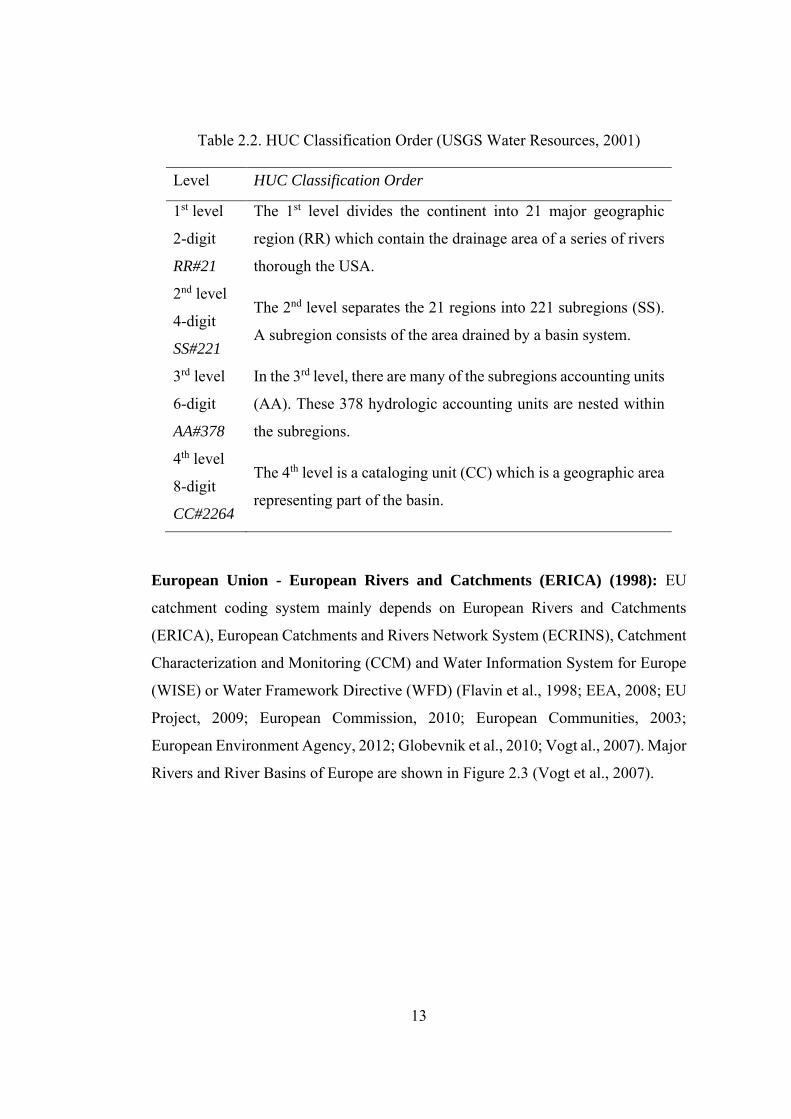
Table 2.2. HUC Classification Order (USGS Water Resources, 2001)
Level HUC Classification Order
1st level
2-digit
RR#21
The 1st level divides the continent into 21 major geographic
region (RR) which contain the drainage area of a series of rivers
thorough the USA.
2nd level
4-digit
SS#221
The 2nd level separates the 21 regions into 221 subregions (SS).
A subregion consists of the area drained by a basin system.
3rd level
6-digit
AA#378
In the 3rd level, there are many of the subregions accounting units
(AA). These 378 hydrologic accounting units are nested within
the subregions.
4th level
8-digit
CC#2264
The 4th level is a cataloging unit (CC) which is a geographic area
representing part of the basin.
European Union - European Rivers and Catchments (ERICA) (1998): EU
catchment coding system mainly depends on European Rivers and Catchments
(ERICA), European Catchments and Rivers Network System (ECRINS), Catchment
Characterization and Monitoring (CCM) and Water Information System for Europe
(WISE) or Water Framework Directive (WFD) (Flavin et al., 1998; EEA, 2008; EU
Project, 2009; European Commission, 2010; European Communities, 2003;
European Environment Agency, 2012; Globevnik et al., 2010; Vogt al., 2007). Major
Rivers and River Basins of Europe are shown in Figure 2.3 (Vogt et al., 2007).
14
Figure 2.3. Major Rivers and River Basins of Europe (Vogt al., 2007)
The ERICA Coding System (ERICA-CS) provides explicit information about areas
draining to a given sea/ocean or coastal stretch in all over the European Continent.
According to the ERICA, the sample code is explained as follows: "MM BBB N1
N2 N3 N4 A" (Flavin et al., 1998).
• "MM" : 2-digit marine code
• "BBB" : 3-digit marine border code
• "N1-N2-N3-N4" : 2-digit nested catchment codes
• "A" : 1 character code driving from area
15
Figure 2.4 depicts the example of the development and demonstration of a structured
hydrological feature coding system that is heavily based on Pfafstetter method for
Europe (de Jager & Vogt, 2010).
Figure 2.4. Pfafstetter Codes for EU (de Jager & Vogt, 2010)
European Catchments and Rivers Network System (ECRINS) (2011) is a very
detailed coding format. It is the newest and most used system in Europe by 2021.
Using the CCM2 (Catchment Characterization and Modeling) GIS database, the data
can be downloaded from internet. The entire European basin database can be
downloaded and used free of charge from the website. Likewise, it can use different
databases. CCM database has been expanding with each passing day and also was
included Turkey in 2009. Large lakes such as Lake Van and Lake Tuz are named
completely in this system. European Environment Agency (EEA) left ERICA and
started to use ECRINS. All major basins in Europe have been defined and coded in
a long list. Nested coding is not allowed. It has a fixed coding system, and its format
is quite long (Globevnik et al., 2010).
16
Water Information System for Europe (WISE) is a reference system for the
ECRINS project. There are also places where WFD (Water Framework Directive) is
written as coding. Object type codes are also valid in this system. Lake, river, etc.
objects can be easily coded with it. Coding is much simpler and clearer than
ECRINS. There is also an expression such as a country code in this code. There is a
serious problem in defining closed basins (Globevnik et al., 2010).
Catchment Characterization and Monitoring (CCM) is a project run by the
European Commission, Joint Research Centre, Institute for Environment and
Sustainability within the scope of providing database and structured hydrological
feature data set on river and catchment codification systems for Europe. Using a
connected data set in which every river basin discharging to sea, one can achieve this
ordering automatically for hydrological feature coding system (Globevnik et al.,
2010).
The Norwegian Register of Catchment Areas (REGINE) is part of the Norwegian
Water Information System (NORWIS), which is developed by the Norwegian Water
Resources and Energy Administration (NVE) (Flavin et al., 1998).
German Catchment Coding System (LAWA) is a kind of hydrological
codification method of catchment coding. It has been established by a committee of
the Länderarbeitsgemeinschaft Wasser (LAWA) (Flavin et al., 1998).
The Finnish codification system (FINISH) in Finland, it is a structured hierarchical
approach and successfully applied to many real practices; however, the ordering
method applying with 18 characters to code river networks results in too complicated
in terms of labeling structure (Britton, 2002). Therefore, it makes hard to code a new
interbasin or tributary which connects and joins together into the networks because
the coded network must be re-coded again and again (Britton, 2002).
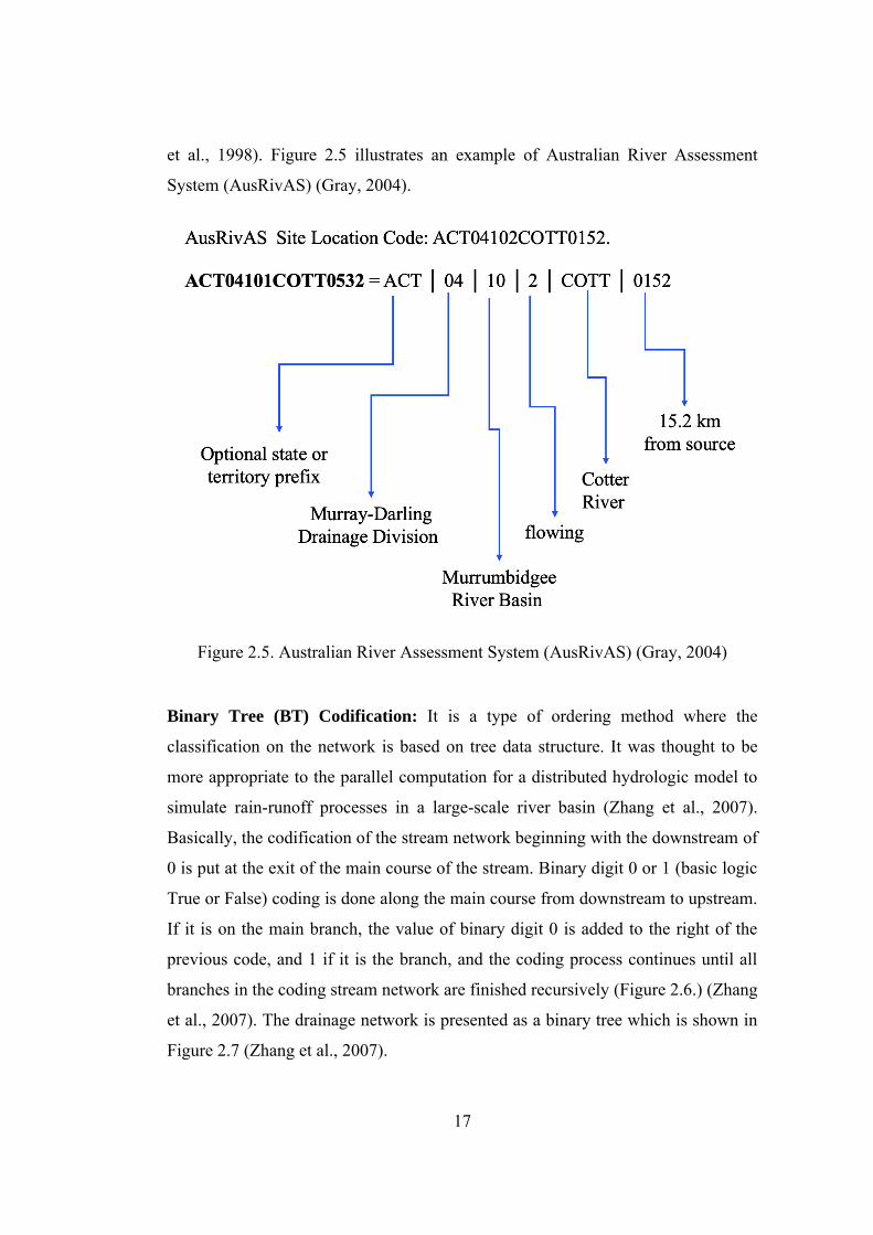
Australian River Assessment System (AusRivAS) is a type of hydrological
codification system that is used for a variety of purposes, water resource condition
auditing, and demonstrating the natural resource and river network situation (Flavin
17
et al., 1998). Figure 2.5 illustrates an example of Australian River Assessment
System (AusRivAS) (Gray, 2004).
Figure 2.5. Australian River Assessment System (AusRivAS) (Gray, 2004)
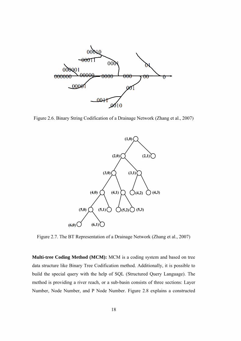
Binary Tree (BT) Codification: It is a type of ordering method where the
classification on the network is based on tree data structure. It was thought to be
more appropriate to the parallel computation for a distributed hydrologic model to
simulate rain-runoff processes in a large-scale river basin (Zhang et al., 2007).
Basically, the codification of the stream network beginning with the downstream of
0 is put at the exit of the main course of the stream. Binary digit 0 or 1 (basic logic
True or False) coding is done along the main course from downstream to upstream.
If it is on the main branch, the value of binary digit 0 is added to the right of the
previous code, and 1 if it is the branch, and the coding process continues until all
branches in the coding stream network are finished recursively (Figure 2.6.) (Zhang
et al., 2007). The drainage network is presented as a binary tree which is shown in
Figure 2.7 (Zhang et al., 2007).
18
Figure 2.6. Binary String Codification of a Drainage Network (Zhang et al., 2007)
Figure 2.7. The BT Representation of a Drainage Network (Zhang et al., 2007)
Multi-tree Coding Method (MCM): MCM is a coding system and based on tree
data structure like Binary Tree Codification method. Additionally, it is possible to
build the special query with the help of SQL (Structured Query Language). The
method is providing a river reach, or a sub-basin consists of three sections: Layer
Number, Node Number, and P Node Number. Figure 2.8 explains a constructed
19
drainage network and MCM of all sub-basins: 1st code component is Layer Number,
2nd is Node Number, and 3rd is P Node Number, respectively (Wang et al., 2013).
Figure 2.8. The Drainage Network with MCM (Wang et al., 2013)
Figure 2.9 depicts the data structure of the basin with MCM coding. For computer
memory, the square demonstrates a type of data collection such as an array and list.
The element stores the physical address of one sub-basin node. The size of array
rows is equal to the size of layers of the tree, and the size of the columns in each
array row is equal to the number of nodes in each multi-tree layer. (Wang et al.,
2013)
Figure 2.9. The Multi-Tree Drainage Network (Wang et al., 2013)
20
Table 2.3 demonstrates the summary of common properties among different
topological encoding schemes being employed in the European Union (Britton,
2002).
Table 2.3. The Comparison of Topological Encoding Systems (Britton, 2002)
The Comparison of Topological Encoding Systems
Coding System
To
polo
gy C
aptu
red
St
ruct
ured
Nes
ted
Ea
sy to
Und
erst
and
Ex
tra D
igit(
s)
H
ydro
logi
cal C
atch
men
t
#N
este
d Su
b-C
atch
men
t
#N
este
d Tr
ibut
ary
In
dica
tes C
atch
men
t
Pfafstetter (USA) + + + + + 9 4 -
ERICA (EU) + + + + + 99 49 +
LAWA (Germany) + + + + + 9 4 -
REGINE (Norway) + + - - - 33 - -
FINISH (Finland) + + - + + - 100 +
21
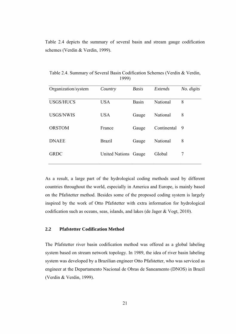
Table 2.4 depicts the summary of several basin and stream gauge codification
schemes (Verdin & Verdin, 1999).
Table 2.4. Summary of Several Basin Codification Schemes (Verdin & Verdin, 1999)
Organization/system Country Basis Extends No. digits
USGS/HUCS USA Basin National 8
USGS/NWIS USA Gauge National 8
ORSTOM France Gauge Continental 9
DNAEE Brazil Gauge National 8
GRDC United Nations Gauge Global 7
As a result, a large part of the hydrological coding methods used by different
countries throughout the world, especially in America and Europe, is mainly based
on the Pfafstetter method. Besides some of the proposed coding system is largely
inspired by the work of Otto Pfafstetter with extra information for hydrological
codification such as oceans, seas, islands, and lakes (de Jager & Vogt, 2010).
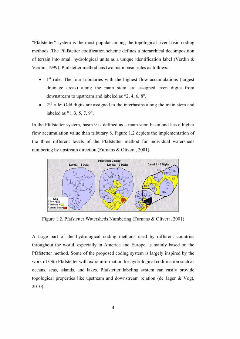
2.2 Pfafstetter Codification Method
The Pfafstetter river basin codification method was offered as a global labeling
system based on stream network topology. In 1989, the idea of river basin labeling
system was developed by a Brazilian engineer Otto Pfafstetter, who was serviced as
engineer at the Departamento Nacional de Obras de Saneamento (DNOS) in Brazil
(Verdin & Verdin, 1999).
22
The Pfafstetter method heavily depends on the topology of the drainage network and
the size of the surface area drained. It provides identification numbers recursively to
the degree of the smallest subbasins extractable from a Digital Elevation Model
(DEM) (Britton, 2002).
Actually, Pfafstetter codification method is a kind of numbering scheme in order to
use labeling drainage networks in a river basin domain (Verdin & Verdin, 1999).
There are two key phenomena in the rules of Pfafstetter codification: "basin"
(drainage area towards to a reach of the main stem) and "interbasin" (between the
drainage areas that drained by any tributaries). An idealized river basin showing
subdivision into coded basins and interbasins is shown in Figure 2.10. If closed
basins (internal basins) are encountered, the largest one is assigned the number zero.
(Verdin & Verdin, 1999).
Figure 2.10. Sample subdivisions of a basin and an interbasin obtained by applying
the rules of Pfafstetter codification (Verdin & Verdin, 1999)
23
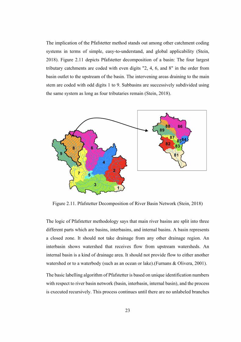
The implication of the Pfafstetter method stands out among other catchment coding
systems in terms of simple, easy-to-understand, and global applicability (Stein,
2018). Figure 2.11 depicts Pfafstetter decomposition of a basin: The four largest
tributary catchments are coded with even digits "2, 4, 6, and 8" in the order from
basin outlet to the upstream of the basin. The intervening areas draining to the main
stem are coded with odd digits 1 to 9. Subbasins are successively subdivided using
the same system as long as four tributaries remain (Stein, 2018).
Figure 2.11. Pfafstetter Decomposition of River Basin Network (Stein, 2018)
The logic of Pfafstetter methodology says that main river basins are split into three
different parts which are basins, interbasins, and internal basins. A basin represents
a closed zone. It should not take drainage from any other drainage region. An
interbasin shows watershed that receives flow from upstream watersheds. An
internal basin is a kind of drainage area. It should not provide flow to either another
watershed or to a waterbody (such as an ocean or lake).(Furnans & Olivera, 2001).
The basic labelling algorithm of Pfafstetter is based on unique identification numbers
with respect to river basin network (basin, interbasin, internal basin), and the process
is executed recursively. This process continues until there are no unlabeled branches
24
for each level. Meanwhile, the direction of the labelling is always from downstream
or outlet (seaside) to upstream or source vice versa flow accumulation. Here is the
basic Pfafstetter labelling steps:
• First of all, determining the path of main stem and tributary is very important
in order to find the right labelling on right way otherwise it is hard to know
whether it is the main stem or tributary. Before igniting the labelling process,
the best practice is double check with lengths and depth values for each level
on the river network. Horton-Strahler method might be helpful to find the
longest or deepest path with respect to high level order ranking.
• Secondly, select the four tributaries according to the largest drainage areas
along the main stem of the river. The four tributaries are marked even digits
through the direction (from the watershed outlet to the source) from
downstream to upstream. The watersheds containing these four tributaries are
basins. Assign each basin the code "2," "4," "6," or "8", the most downstream
basin gets the "2", the next most downstream basin gets the "4" and so on
(Furnans & Olivera, 2001).
• Thirdly, assign odd digits to the interbasins along the main stem of the river
network. Marking each interbasin the code "1," "3," "5," "7," or "9" in the
upstream direction, the most downstream interbasin gets "1," the next most
downstream interbasin gets "3," etc. Therefore, interbasins are the watersheds
between basins. Due to the power of network topology, in the Pfafstetter
system, basin 9 is defined as a main stem basin and has a higher flow
accumulation value than tributary 8 (The National Severe Storms Laboratory
(NSSS), 2004). Figure 2.12 depicts the steps of Pfafstetter labelling (de
Bartolo et al., 2009).
25
Figure 2.12. The Tributary Basin Pfafstetter Number (2, 4, 6, 8) (a); The Pfafstetter Labelling Direction (b); The Main Stem Interbasin Pfafstetter Number (1, 3, 5, 7,
9) (c) (NSSS, 2004)
Even if there are less than four tributaries in the system of Pfafstetter labelling, the
number of basins "9" is always the main stem of the river network (Figure 2.13)
(NSSS), 2004). Additionally, if an area contains internal basins, the largest internal
basin is assigned the code "0" and all other internal basins are incorporated into a
surrounding basin or interbasin (de Bartolo et al., 2009).
Figure 2.13. Pfafstetter Codification (less than four basins or interbasins) (NSSS,
2004)
(a) (b) (c)
26
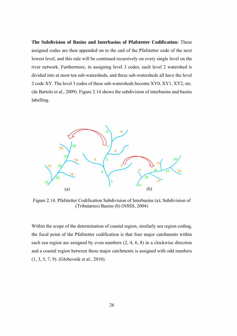
The Subdivision of Basins and Interbasins of Pfafstetter Codification: These
assigned codes are then appended on to the end of the Pfafstetter code of the next
lowest level, and this rule will be continued recursively on every single level on the
river network. Furthermore, in assigning level 3 codes, each level 2 watershed is
divided into at most ten sub-watersheds, and these sub-watersheds all have the level
2 code XY. The level 3 codes of these sub-watersheds become XY0, XY1, XY2, etc.
(de Bartolo et al., 2009). Figure 2.14 shows the subdivision of interbasins and basins
labelling.
Figure 2.14. Pfafstetter Codification Subdivision of Interbasins (a); Subdivision of
(Tributaries) Basins (b) (NSSS, 2004)
Within the scope of the determination of coastal region, similarly sea region coding,
the focal point of the Pfafstetter codification is that four major catchments within
each sea region are assigned by even numbers (2, 4, 6, 8) in a clockwise direction
and a coastal region between these major catchments is assigned with odd numbers
(1, 3, 5, 7, 9). (Globevnik et al., 2010).
(a) (b)
27
The disadvantage of Pfafstetter coding is being limited to the maximum 9 basins, if
there are more than 4 main branches, the remaining branches should be ignored. On
the other hand, the method of Pfafstetter provides the robust topological capability
through the river network. There are also modified uses especially in the EU (Verdin
& Verdin, 1999). In other words, this method can be used by modifying it as desired.
All over the world, most of the hydrological coding methods are heavily based on
the Pfafstetter methodology.
Topological Characteristics of the Pfafstetter Codification: Pfafstetter digits
indicate relative upstream and downstream positions at the river network. Therefore,
these numbers can be used for providing more detail and clearer picture in terms of
basin topological analyses. The more we use the combination of Digital Elevation
Models (DEM) and subsequent exploitation with both Database Management
System (DBMS) and Geographic Information Systems (GIS) software, the better and
more robust network topology can be obtained (Furnans & Olivera, 2001). Assuming
that there is no topological feature, Pfafstetter or similar hydrological coding
methods will lack a relational feature for any network structure. In fact, the
application of Pfafstetter coding is due to the strength of topology in the river
network.
In order to manage topology, we need to know relationship among the input network
data. The Pfafstetter ID number provide sufficient information about the correlation
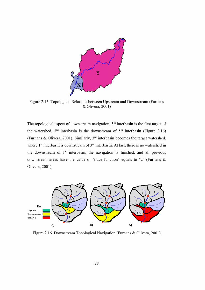
between upstream and downstream. Figure 2.15 demonstrates that the topological
relations in terms of upstream and downstream are relative to location. The area of
X is at the downstream of the area of Y; therefore, one can be said that the location
of Y must be the upstream of X respectively (Furnans & Olivera, 2001).
28
Figure 2.15. Topological Relations between Upstream and Downstream (Furnans
& Olivera, 2001)
The topological aspect of downstream navigation, 5th interbasin is the first target of
the watershed, 3rd interbasin is the downstream of 5th interbasin (Figure 2.16)
Pfafstetter codification scheme defines a hierarchical decomposition of a terrain into
small hydrological units as a unique identification label (Verdin & Verdin, 1999).
Pfafstetter method can easily apply on the river network by using unique numbers.
These numbers represent topological properties in terms of upstream and
downstream adjacency and neighborhood (Karaman et al., 2019).
Some example applications are selected from the famous river networks in the world.
The Amazon River Basin in South America and the Thames River Catchment in the
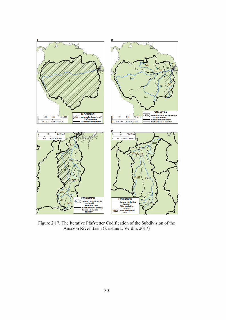
UK are presented. Figure 2.17 explains that Pfafstetter subdivision of the Amazon
River Basin. Figure 2.17 explains the Pfafstetter subdivision of the Amazon River
Basin as follows:
• Firstly, in Pfafstetter Level-1, Amazon River Basin is assigned with the
Pfafstetter code 54. The digit of 5 is the continental number (South America),
and 4 is the 1st level of the Pfafstetter label for the Amazon Basin (A).
• Secondly, in Pfafstetter Level-2, Amazon River Basin is divided into
subdivisions of the basins to identify the largest four tributaries. Amazon
River is labeled with even numbers (2, 4, 6, 8). The headwaters of the
subbasin are 9 (source), and the interbasins are assigned with odd digits (1,
3, 5, 7) (B).
• Thirdly, in Pfafstetter Level-3, The subdivisions of the Amazon River Basin
are assigned with the even (four largest tributaries) and odd digits
(interbasins) recursively like level-2. For each iteration, 9 must be labeled
with source (C).
• Lastly, in Pfafstetter Level-4, the four biggest tributaries are labeled with
even numbers (2, 4, 6, 8) again. As always 9 is the headwaters for the basin
of 5422. The interbasins are assigned with odd numbers (1, 3, 5, 7) (D)
(Kristine L Verdin, 2017).
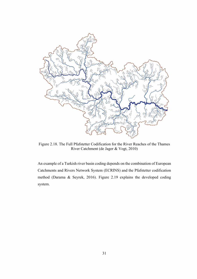
Similarly, Figure 2.18 depicts different level of Pfafstetter codification for the
Thames River Basin (de Jager & Vogt, 2010).
30
Figure 2.17. The Iterative Pfafstetter Codification of the Subdivision of the
Amazon River Basin (Kristine L Verdin, 2017)
31
Figure 2.18. The Full Pfafstetter Codification for the River Reaches of the Thames
River Catchment (de Jager & Vogt, 2010)
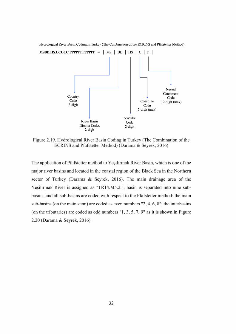
An example of a Turkish river basin coding depends on the combination of European
Catchments and Rivers Network System (ECRINS) and the Pfafstetter codification
method (Darama & Seyrek, 2016). Figure 2.19 explains the developed coding
system.
32
Figure 2.19. Hydrological River Basin Coding in Turkey (The Combination of the
ECRINS and Pfafstetter Method) (Darama & Seyrek, 2016)
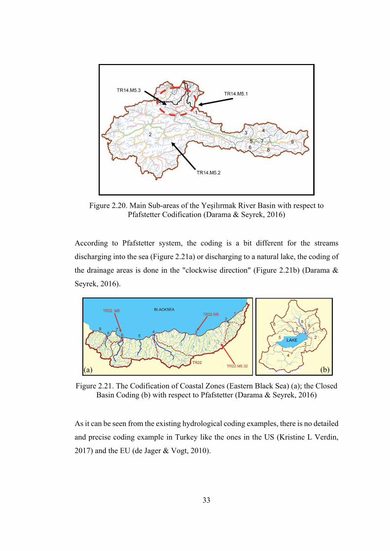
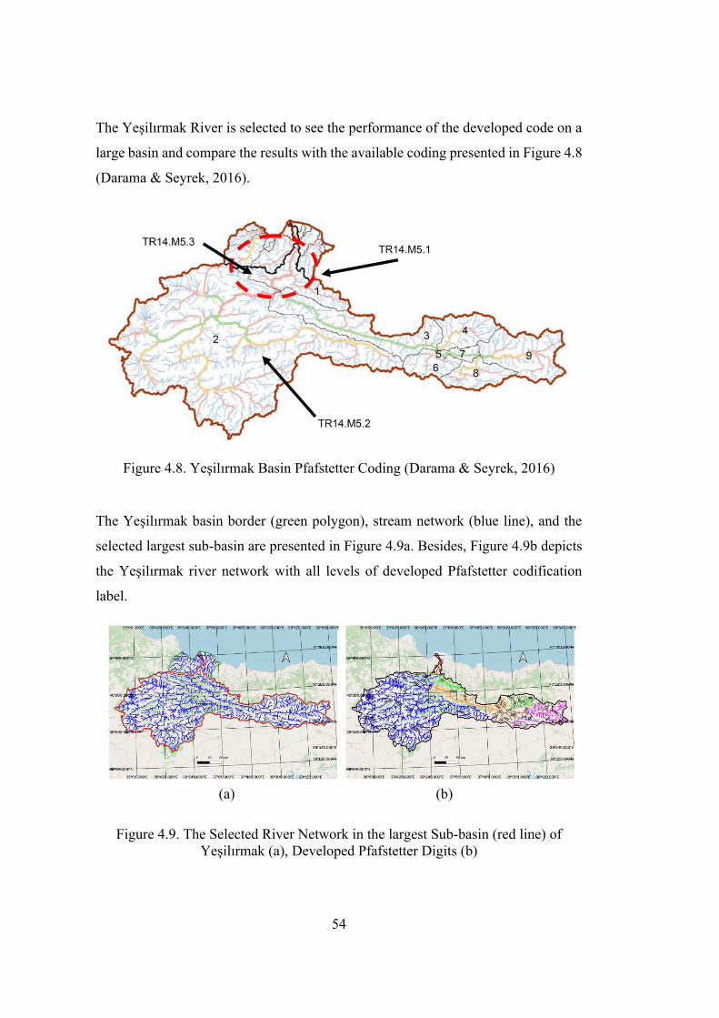
The application of Pfafstetter method to Yeşilırmak River Basin, which is one of the
major river basins and located in the coastal region of the Black Sea in the Northern
sector of Turkey (Darama & Seyrek, 2016). The main drainage area of the
Yeşilırmak River is assigned as "TR14.M5.2.", basin is separated into nine sub-
basins, and all sub-basins are coded with respect to the Pfafstetter method: the main
sub-basins (on the main stem) are coded as even numbers "2, 4, 6, 8"; the interbasins
(on the tributaries) are coded as odd numbers "1, 3, 5, 7, 9" as it is shown in Figure
2.20 (Darama & Seyrek, 2016).
33
Figure 2.20. Main Sub-areas of the Yeşilırmak River Basin with respect to Pfafstetter Codification (Darama & Seyrek, 2016)
According to Pfafstetter system, the coding is a bit different for the streams
discharging into the sea (Figure 2.21a) or discharging to a natural lake, the coding of
the drainage areas is done in the "clockwise direction" (Figure 2.21b) (Darama &
Seyrek, 2016).
Figure 2.21. The Codification of Coastal Zones (Eastern Black Sea) (a); the Closed
Basin Coding (b) with respect to Pfafstetter (Darama & Seyrek, 2016)
As it can be seen from the existing hydrological coding examples, there is no detailed
and precise coding example in Turkey like the ones in the US (Kristine L Verdin,
2017) and the EU (de Jager & Vogt, 2010).
(a) (b)
35
CHAPTER 3
3 METHODOLOGY
3.1 Methodology
The network data structure is one of the most important phenomena that is mainly
based on two kinds of mathematical disciplines: network and topology (how the
segments in the network are connected to each other) (Demšar et al., 2008). The
power of the topological relationships led to revolutionary advances in GIS,
especially at network applications like river basin coding (Curtin, 2007). Basically,
the methodology consists of four key elements: GIS, data structure, network, and
topology. In the field of hydrology, the Pfafstetter labeling system stands out as the
most well-known and popular coding method all over the world. The river network
data structure heavily depends on the binary tree data structure. What is more, "trees"
are graphs those have the following attributes (Celko, 2012):
• A tree is a connected graph that has no cycles. A connected graph is one in
which there is a path between any two nodes. No node sits by itself,
disconnected from the rest of the graph.
• Every node is the root of a subtree, and the most trivial case is a subtree of
only one node.
• Every two nodes in the tree are connected by one and only one path. In a tree,
the number of edges is one less than the number of nodes.
Within the scope of the data structure of the river network, "binary tree" is a kind of
tree, and it has the following characteristics (Goodrich et al., 2013):
• Every node has at most two children. Each child node is marked as either left
child or right child.
• A left child precedes a right child in the order of children of a node.
36
The subtree rooted at either left or right child of an internal node is named as a left
or right subtree, respectively (Goodrich et al., 2013). Furthermore, it might be
possible to put spatial relationships on this data model as shown in Figure 3.1 (Demir
& Szczepanek, 2017), and in Figure 3.2 (Arge et al., 2006).
Figure 3.1. Binary Tree Data Model (a); Topology of River Network Codification Proposed by Pfafstetter (b); Stream Network Data Structure Model (c) (Demir &
Szczepanek, 2017)
(a) (b)
(c)
37
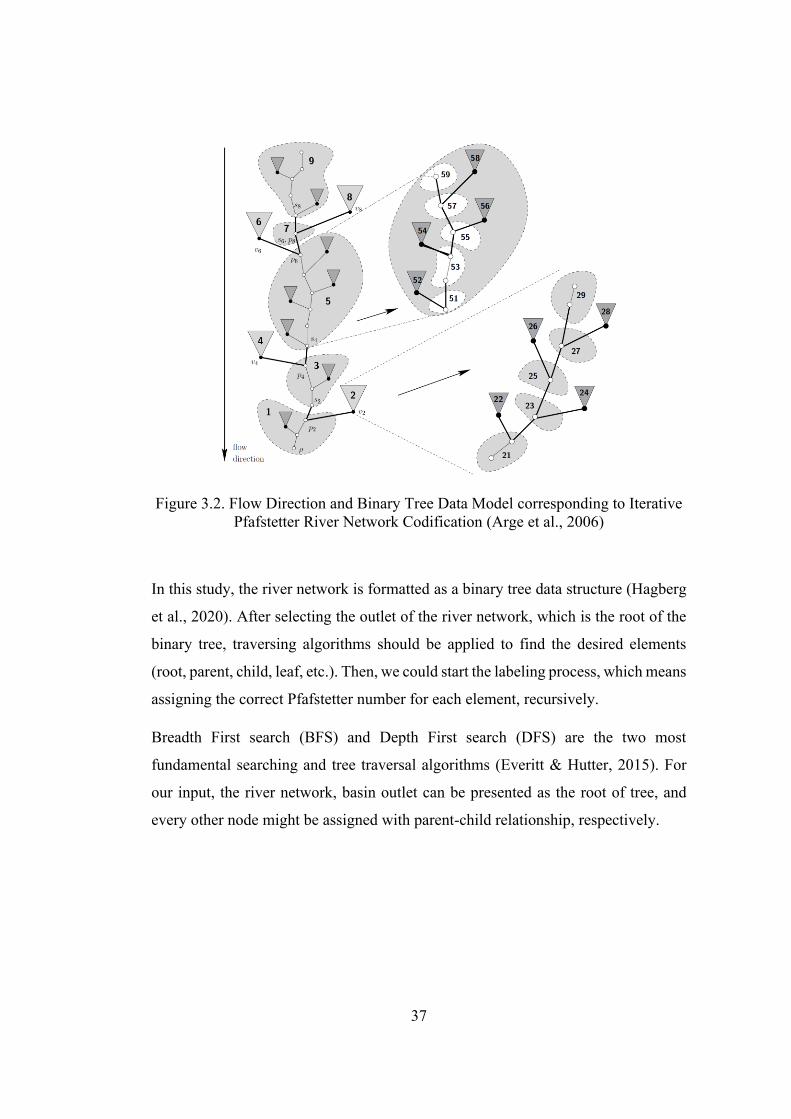
Figure 3.2. Flow Direction and Binary Tree Data Model corresponding to Iterative
Pfafstetter River Network Codification (Arge et al., 2006)
In this study, the river network is formatted as a binary tree data structure (Hagberg
et al., 2020). After selecting the outlet of the river network, which is the root of the
binary tree, traversing algorithms should be applied to find the desired elements
(root, parent, child, leaf, etc.). Then, we could start the labeling process, which means
assigning the correct Pfafstetter number for each element, recursively.
Breadth First search (BFS) and Depth First search (DFS) are the two most
fundamental searching and tree traversal algorithms (Everitt & Hutter, 2015). For
our input, the river network, basin outlet can be presented as the root of tree, and
every other node might be assigned with parent-child relationship, respectively.
38
3.1.1 Workflow
The workflow for computing the river networks in Pfafstetter codification algorithm
is demonstrated in Figure 3.3.
Figure 3.3. The Workflow for Computing the River Networks in the Pfafstetter Codification Algorithm
The flow of process consists of three main steps of action in order to execute the
developed codification algorithm.
1st step is called as "Watershed (Catchment)" which is constructed by SAGA,
GRASS, and GDAL tools in QGIS software and plug-in. First of all, Digital
Elevation Model (DEM) is obtained from NASA Shuttle Radar Topography Mission
(SRTM) Global 1 arc-second (about 30 meters) (NASA, 2020). After interpolating
voids and filling missing data in DEM for catchment delineation with using Raster
analysis tools in GDAL, filling the sinks algorithm in SAGA tools (Terrain Analysis
-> Hydrology) is used. Strahler order of the river network can be obtained with
SAGA -> Terrain Analysis -> Channels in QGIS.
39
2nd step is called as "River (Channel or Stream) Network". This is built via SAGA
and GRASS tools in QGIS domain. By using SAGA tools (SAGA -> Terrain
Analysis -> Channels -> Channel Network & Drainage Basins), we can get some
outputs such as Flow Direction, Drainage Basin (raster), Channels, and Drainage
Basin (vector). Similarly, stream and catchment delineation can be built via GRASS
tools (Figure 3.4.) (Jasiewicz & Metz, 2011).
Figure 3.4. The Structure of the GRASS and Data Flow Between Particular
Modules and External Software (Jasiewicz & Metz, 2011)
Figure 3.5. shows the details of the operations performed in the above two steps in
order to reach the river network (Lauermann et al., 2016).
40
Figure 3.5. Workflow for the Channel Networks in SAGA and GRASS
(Lauermann et al., 2016)
3rd step is called as "Pfafstetter Codification Algorithm". It is coded by python
programming language. The developed software can be embedded in GIS
applications.
The mathematical model of this study is constructed with using python builder in
QGIS software, main outputs of the model are Filled DEM, River Network, and Root
Node (outlet), which are shown as boxes with green background in Figure 3.6. The
source python code of the model is shown in Appendix-A (QGIS, 2020).
41
Figu
re 3
.6. M
athe
mat
ical
Mod
el u
sed
in Q
GIS
Sof
twar
e in
the
Stud
y
42
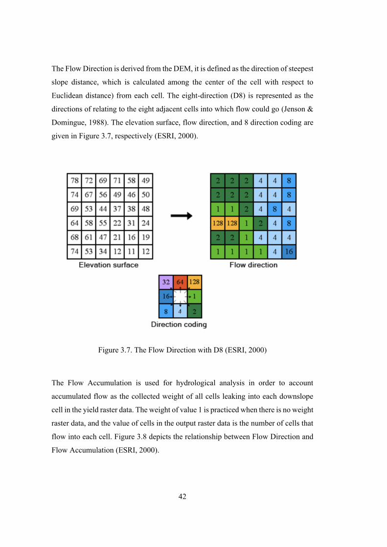
The Flow Direction is derived from the DEM, it is defined as the direction of steepest
slope distance, which is calculated among the center of the cell with respect to
Euclidean distance) from each cell. The eight-direction (D8) is represented as the
directions of relating to the eight adjacent cells into which flow could go (Jenson &
Domingue, 1988). The elevation surface, flow direction, and 8 direction coding are
given in Figure 3.7, respectively (ESRI, 2000).
Figure 3.7. The Flow Direction with D8 (ESRI, 2000)
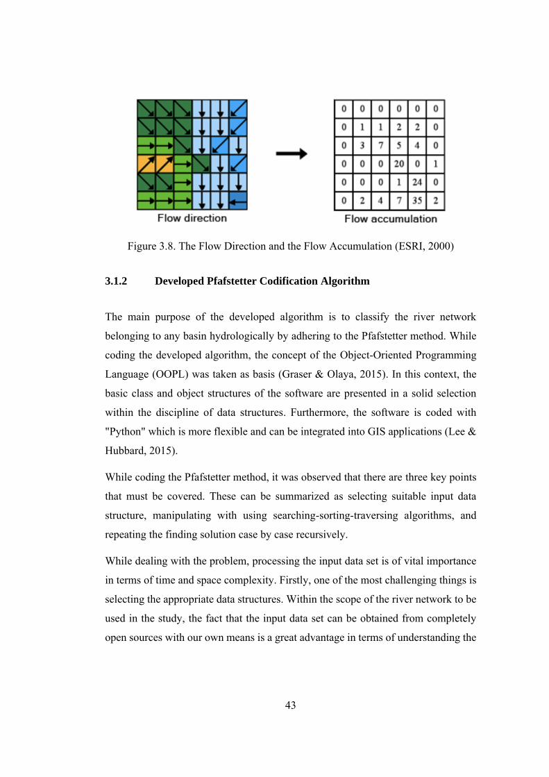
The Flow Accumulation is used for hydrological analysis in order to account
accumulated flow as the collected weight of all cells leaking into each downslope
cell in the yield raster data. The weight of value 1 is practiced when there is no weight
raster data, and the value of cells in the output raster data is the number of cells that
flow into each cell. Figure 3.8 depicts the relationship between Flow Direction and
Flow Accumulation (ESRI, 2000).
43
Figure 3.8. The Flow Direction and the Flow Accumulation (ESRI, 2000)
3.1.2 Developed Pfafstetter Codification Algorithm
The main purpose of the developed algorithm is to classify the river network
belonging to any basin hydrologically by adhering to the Pfafstetter method. While
coding the developed algorithm, the concept of the Object-Oriented Programming
Language (OOPL) was taken as basis (Graser & Olaya, 2015). In this context, the
basic class and object structures of the software are presented in a solid selection
within the discipline of data structures. Furthermore, the software is coded with
"Python" which is more flexible and can be integrated into GIS applications (Lee &
Hubbard, 2015).
While coding the Pfafstetter method, it was observed that there are three key points
that must be covered. These can be summarized as selecting suitable input data
structure, manipulating with using searching-sorting-traversing algorithms, and
repeating the finding solution case by case recursively.
While dealing with the problem, processing the input data set is of vital importance
in terms of time and space complexity. Firstly, one of the most challenging things is
selecting the appropriate data structures. Within the scope of the river network to be
used in the study, the fact that the input data set can be obtained from completely
open sources with our own means is a great advantage in terms of understanding the
44
input data structure and choosing the most suitable data structure. Thus, it has been
determined that the data structure has binary tree properties.
After selecting the outlet of the river network, which is the root of the binary tree,
traversing algorithms should be applied to find the desired elements (root, parent,
child, leaf, etc.). Then, we could start the labeling process, which means assigning
the correct Pfafstetter number for each element, recursively.
Although there are many traversing algorithms for tree structures in the literature,
the most well-known ones are Depth First Search (DFS) and Breadth First Search
(BFS). Due to the unbalance structure of the river network, the DFS algorithm in
which priority goes to the deepest node is preferred in terms of performance.
Eventually, in order to code all the elements in the tree structure in accordance with
the Pfafstetter logic, we need to define different situations to respond to all options
on the table. To solve the problem recursively, in accordance with the Pfafstetter
method (1st rule: tributaries are assigned as "2, 4, 6, 8" with respect to the selected
largest four drainage areas; 2nd rule: main stems are labeled as "1, 3, 5, 9", note that
1 and 9 must always be labeled) four base cases were determined at the beginning.
These cases were determined based on the depth of the tree (Figure 3.9). Considered
in the binary tree data structure, the main tree consists of sub-trees. Therefore, the
major tree might be adapted by sub-tree owing to the suitable cases with respect to
tree depth, recursively.
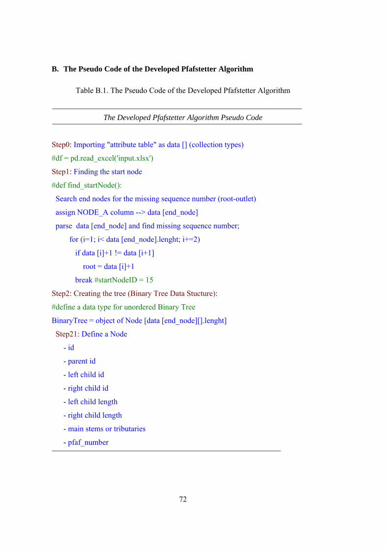
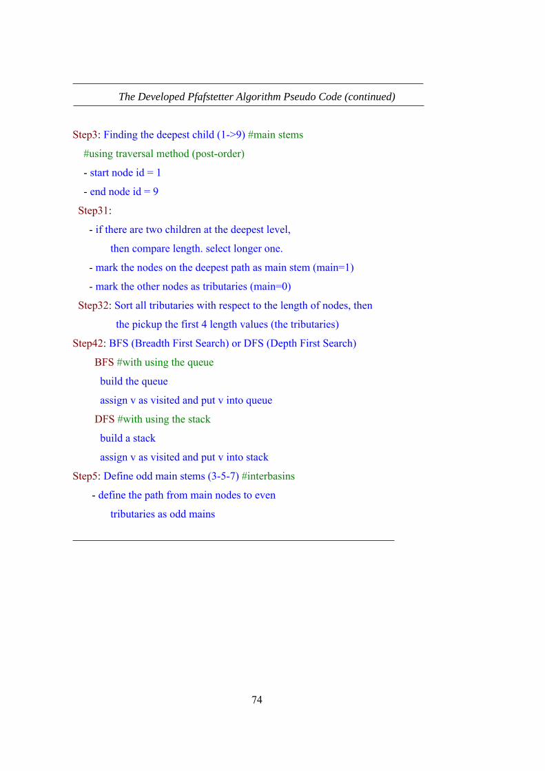
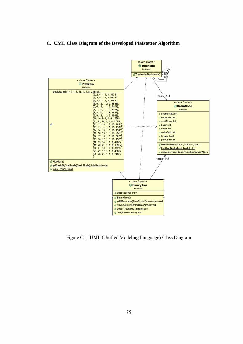
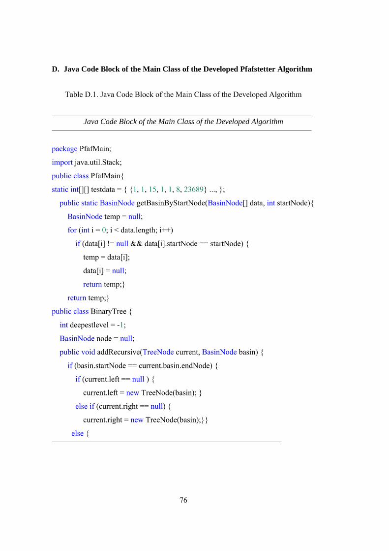
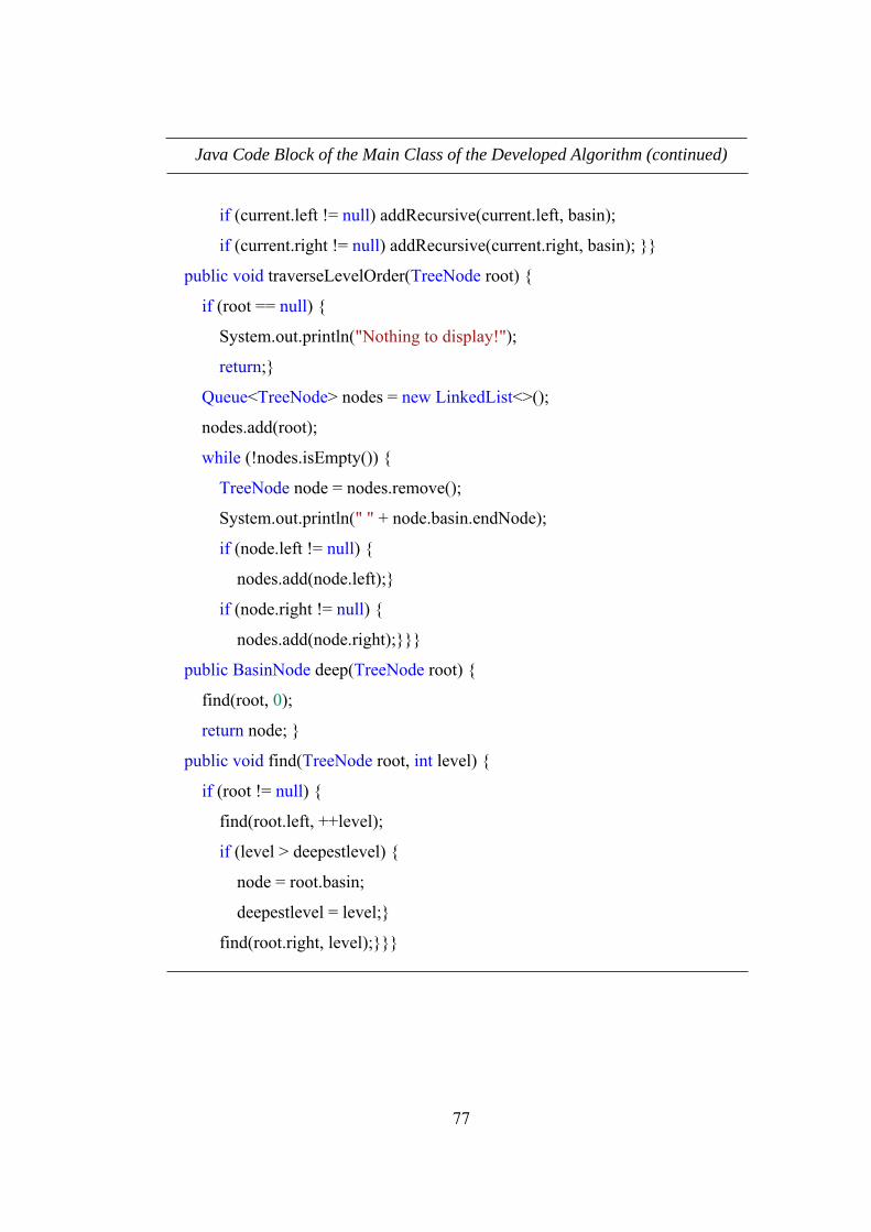
Unified Modeling Language (UML) class diagram, the pseudo code, and the main
class of the developed Pfafstetter algorithm are shown in Appendix-B, Appendix-C,
and Appendix-D, respectively.
45
Figure 3.9. All Basic Cases of Developed Pfafstetter Algorithm
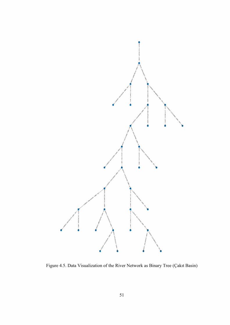
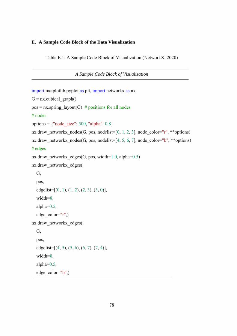
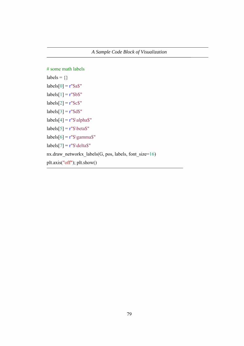
3.1.3 Data Visualization of the River Network Structure
In order to better analyze the accuracy of the results of the developed code, the code
block is encoded in the python language using the Network-X library (sample code
block is shown in Appendix-E) (NetworkX, 2020). It is aimed to display the whole
picture in a more understandable and practical way.
47
CHAPTER 4
4 RESULTS AND DISCUSSION
In this chapter, the outcomes of the developed Pfafstetter algorithm are presented for
selected three different river basins, which are Çakıt basin in Adana (the southern
part of Turkey), Yeşilırmak basin (the northern part of Turkey), and Thames River
basin in London (the southern part of England). Similarities and differences between
the results of this study and other studies in the literature are discussed.
4.1 The Çakıt Basin
Çakıt Basin, which is a branch of the Seyhan river, pours into the Seyhan reservoir.
The largest tributary of Çakıt River is nearly 40 km long. The map of Turkey
showing Çakıt Basin is shown in Figure 4.1.
Figure 4.1. The Çakıt River Basin
Within the scope of stream delineation in QGIS using SAGA and GRASS tools,
different threshold values were selected, while obtaining Çakıt river network at a
scale 1/25000. One can also choose the default values for both GIS tools. Stream
48
network of the basin is created by SAGA (blue lines) and GRASS (red lines) tools
in QGIS from SRTM DEM (Figure 4.2).
Figure 4.2. The Çakıt Stream Network
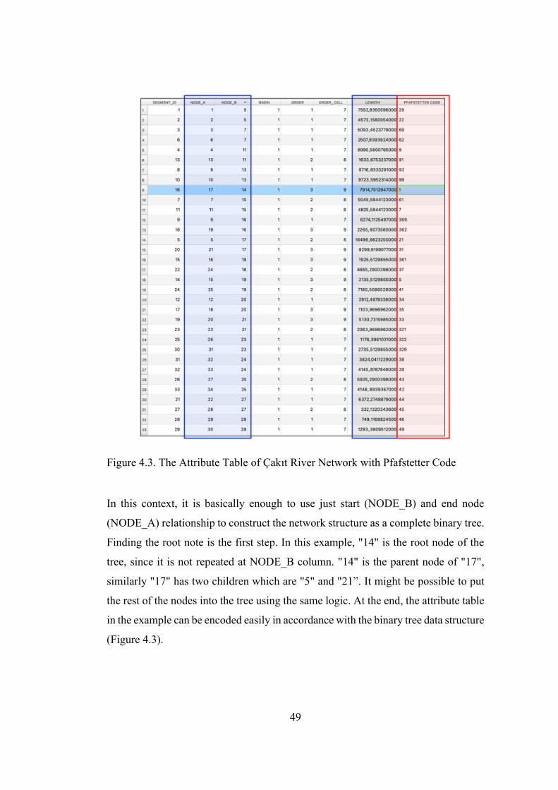
The first part of the attribute table [SEGMENT_ID (Unique ID), NODE_A (End